Abstract

The conductivity of a finite temperature 1+1 dimensional fermion gas described by the massive Thirring model is shown to be related to the retarded propagator of the dual boson sine-Gordon model. Duality provides a natural resummation which resolves infra-red problems, and the boson propagator can be related to the fermion gas at non-zero temperature and chemical potential or density. In addition, at high temperatures, we can apply a dimensional reduction technique to find resummed closed expressions for the boson self-energy and relate them to the fermion conductivity. Particular attention is paid to the discussion of analytic continuation. The resummation implicit in duality provides a powerful alternative to the standard diagrammatic evaluation of transport coefficients at finite temperature.

1 Introduction and motivation

The evaluation of transport coefficients at high temperatures in terms of Feynman diagrams in a weakly coupled theory is a subtle and highly involved task [1, 2]. Firstly, they are often proportional to the mean free path of the scattering processes, which increases as coupling strength decreases. Further, in the relevant limits of vanishing external momenta and energy, higher loop diagrams can be as important as lower loop diagrams if they are sufficiently infrared sensitive. The failure of perturbation theory that both of these observations imply requires careful and clever resummation of diagrams.

In lower dimensions we know that this resummation is a reflection of the fact that the relevant degrees of freedom are not those of the quasi-particles, but of dual degrees of freedom. This is well understood in the case of Luttinger liquids, electrons close to the Fermi surface in one dimension (quantum wires). Such a system [3, 4, 5] has a dual representation of its charge modes in terms of free bosonic fields, which provide the relevant degrees of freedom. This leads to a huge simplification in the calculation of conductivity [6], not easily visible (if at all) from electron Feynman diagrams. The predictions that this simple duality permits have been confirmed in experimental measurements [7] of the conductance of $GaAs$ quantum wires, although the finiteness of the system enforces a modification [8] of the naive picture.

In this work we explore the advantages of using this fermion-boson duality when calculating conductivity for relativistic quantum fields in 1+1 dimensions. The hope is that the infinite-order non-perturbative resummation of the quasi-particle modes can be replaced by a few terms in the series for the dual degrees of freedom i.e. that duality does the resummation for us. Further, the usual calculation of transport coefficients relies on linear response theory, and the simplifications implicit in the dual resummation suggest that we can go beyond linear response, otherwise impossible.

As our example, we will concentrate on perhaps the simplest non-trivial theory displaying conductivity: the Massive Thirring (MT) fermion theory, with Minkowski Lagrangian density

$${\cal{L}}_{MT}[\bar{\psi},\psi]=\bar{\psi}(i\not{\!{\partial}}-m_{0})\psi-\frac{1}{2}g^{2}j_{\mu}(x)j^{\mu}(x),$$ (1.1)

where $j_{\mu}=(\rho,j)=\bar{\psi}\gamma_{\mu}\psi$ is the fermion number current.

This is dual to the sine-Gordon (SG) boson model, which is described by

$${\cal L}_{SG}[\phi]=\frac{1}{2}\partial_{\mu}\phi\partial^{\mu}\phi-\frac{\alpha_{0}}{\lambda^{2}}\cos(\lambda\phi).$$ (1.2)

provided the renormalised coupling constants are identified as

$$\frac{\lambda^{2}}{4\pi} = \frac{1}{1+g^{2}/\pi},$$ (1.3)

$$\frac{\alpha}{\lambda^{2}} = \rho m,$$ (1.4)

where $\rho$ is the renormalisation scale and $m$ the renormalised fermion mass.

We note that, with multiplicative renormalisation, if $m_{0}=0$, then the massless Thirring model is dual to the free bosonic field. If we introduce a chemical potential for the fermion field then, in the limit of no antiparticles, we recover the Luttinger limit. However, in QFT the massless limit is unnatural for quarks or electrons and we are obliged to be more sophisticated.

While 1+1 dimensions may seem unrealistic in relativistic quantum field theory, the links of our model with conformal field theory means that these results are relevant to more exotic situations. For instance the study of decay of quantum normal modes of a classical field in the presence of a black hole, all in AdS space, can be linked through AdS/CFT correspondence to linear response in a conformal field theory in 1+1 dimensions [9].

Further, as a precursor to understanding the deconfinement transition in QCD in 3+1 dimensions, the two-dimensional fermionic Thirring model can be put in correspondence with a compact $U(1)$ gauge theory in four dimensions [10], by virtue of Parisi-Sourlas dimensional reduction [11]. From this viewpoint the chiral bilinears of the MT theory correspond to the monopole-antimonopole pairs of the four-dimensional theory, and the monopole condensation that signals confinement has its counterpart in the chirally broken phase of the MT theory [12], that we discussed in detail in an earlier exploration of this duality [13].

In [14, 15] it has been shown that the SG/MT models are also equivalent at finite temperature $T$ and fermion chemical potential $\mu$. Here, we will consider the fermion response to an electric external field (conductivity) as a working example of the use of duality and dimensional reduction in the calculation of transport coefficients. This amounts to an evaluation of the full retarded boson propagator. In this way, the self-energy of the bosons is directly related to the conductivity and charge screening of the fermions. Furthermore, we will show how to relate the dynamical information contained in the boson self-energy, calculated in the imaginary-time (IT) formalism, to the static properties of the fermion gas. In addition, we will use dimensional reduction techniques to analyse the boson propagator. Dimensional reduction is meant to be valid at high temperatures compared to the fermion mass, strong fermion couplings and large distances compared to the inverse temperature. This regime has been shown to be very useful in [13], where it was used to resum exactly the pressure and the fermion condensate at finite $T$ and $\mu$.

The structure of the paper is the following. In section 2 we derive the relationship between the fermion induced currents in linear response theory and the SG retarded propagator. The retarded propagator can be read off from the IT one by analytic continuation. We devote section 3 to analyse the imaginary-time SG propagator. First, we write it as an infinite sum of mass insertions and then we explore its relevant properties and the relationship with the fermion gas at finite chemical potential. In section 4 we discuss the high temperature limit and the dimensional reduction regime for the SG propagator. Analytic continuation from imaginary energy to real energy is a fraught exercise, and this model is simple enough to show how subtle one needs to be. This will become clear in sections 4 and 5 where we will relate the analytic continuation of the high $T$ propagator with the physical conductivity. We will show that one needs to impose physical conditions on the propagator in order to have a physically meaningful answer for the transport coefficients. Many details of the calculation have been collected in the Appendices. Appendix A contains some useful results about thermal propagators and analytic continuation, while Appendix B contains some details of the calculations performed for the SG propagator.

2 Induced fermion currents and the boson retarded propagator

In practice, the only transport coefficient that we will study is electrical conductivity, $\sigma$, the response of electric currents to an electric field, since it is for this that duality can be easily exploited. In our case, the electric field will be an external classical field appearing as a $c$-number source in our action. It is convenient to absorb the gauge coupling $e$ into the gauge fields so that the covariant derivatives are $D^{\mu}=\partial^{\mu}-iA^{\mu}$ and the gauge field has dimension one. The interaction term added to the MT Lagrangian density is then of the form

$$\delta V(t)=j_{\mu}(x,t)A^{\mu}_{cl}(x,t),$$ (2.1)

where the external classical electro-magnetic potential is $A^{\mu}_{cl}$ and $j_{\mu}=(\rho,j)=\bar{\psi}\gamma_{\mu}\psi$ is the fermion number current. Note that using these conventions, the gauge field kinetic term is of the form $-F^{\mu\nu}F_{\mu_{\nu}}/(4e^{2})$ so the electric charge, $e$, has dimensions of energy. As a gauge choice, we will take $A_{1}^{cl}=0$ in what follows, so that the external electric field is

$$E^{cl}(x,t)=-(\partial/\partial x)A_{0}^{cl}(x,t).$$ (2.2)

with dimension two. The electric field satisfies Maxwell’s equations in 1+1 dimensions, which read

$$e^{2}j_{cl}(x,t) = -\dot{E}_{cl}(x,t)$$

$$e^{2}\rho_{cl}(x,t) = \frac{\partial E_{cl}(x,t)}{\partial x}.$$ (2.3)

With these conventions the conductivity $\sigma$ is defined by

$$j=\sigma E,$$ (2.4)

where $j$ is the current density and $E$ is the electric field. The plasma is isotropic and homogeneous so the conductivity is a simple scalar.

In defining conductivity, we are implying that the response of the plasma to an electric field is simply linear in that field. This weak field limit is calculated in quantum field theory using the theory of linear response (see [16, 17]). In terms of the additional interaction term, $\delta V$, of (2.1), the terms linear in electric field come from the first term of a perturbative expansion in powers of $\delta V$. From linear response theory this is then:

$$\langle\langle\delta^{(1)}j_{\mu}(x,t)\rangle\rangle=-i\int_{t_{0}}^{\infty}dt^{\prime}\int_{-\infty}^{\infty}dx^{\prime}A_{0}^{cl}(x^{\prime},t^{\prime})\langle\langle[j_{\mu}(x,t),j_{0}(x^{\prime},t^{\prime})]\rangle\rangle\theta(t-t^{\prime}).$$ (2.5)

The $\delta j_{\mu}(x,t)$ is the difference between the currents with and without the external perturbation. The $\delta^{(1)}$ indicates that it is the term linear in $\delta V$, and hence linear in the electric field. $\langle\langle\cdot\rangle\rangle$ stands for a thermal average taken with respect to an equilibrium density matrix based on the unperturbed Hamiltonian given at time earlier than $t_{0}\in\mathbb{R}$. The perturbation, $\delta V$ is assumed to be switched on only after $t_{0}$ and we are looking at the induced current perturbation at time $t\in\mathbb{R}>t_{0}$.

For the MT model of (1.1), any thermal average involving the fermion current $j_{\mu}$ can be replaced by a boson thermal average in the sine-Gordon model of (1.2). Duality means the fermion current has an exact representation in terms of the scalar SG field alone, namely

$$j_{\mu}(x,t)=\frac{\lambda}{2\pi}\epsilon_{\mu\nu}\partial^{\nu}\phi(x,t),$$ (2.6)

with $\lambda$ defined through (1.3). The proof of the above statement can be found in [15]. If the fermion fields interact electromagnetically, then we would identify $g=O(e)$ in the effective theory described by (1.1). We feel no need to make this identification, and treat $g$ as an independent parameter to be varied irrespective of $e$.

Putting this together for the current then gives

$$\langle\langle\delta^{(1)}j_{1}(x,t)\rangle\rangle=+i\left(\frac{\lambda}{2\pi}\right)^{2}\int_{t_{0}}^{\infty}dt^{\prime}\int_{-\infty}^{\infty}dx^{\prime}A_{0}^{cl}(x^{\prime},t^{\prime})\theta(t-t^{\prime})\frac{\partial}{\partial t}\frac{\partial}{\partial x^{\prime}}\langle\langle[\phi(x,t),\phi(x^{\prime},t^{\prime})]\rangle\rangle.$$ (2.7)

Using integration by parts on the $x^{\prime}$ variable and using (2.2) gives an expression in terms of the electric field. A resulting boundary term at spatial infinity can be ignored in practical problems. The time derivative can be made to act on both expectation value and theta function by using the equal-time commutation relation $[{\phi}(x,t),\phi(x^{\prime},t)]=0$. This then leaves us with the linear response of the fermionic current in terms of the applied electric field given in terms of the full real-time retarded propagator $\Delta_{R}(x,t)$ of the sine-Gordon scalar field

$$\langle\langle\delta^{(1)}j_{1}(x,t)\rangle\rangle=i\left(\frac{\lambda}{2\pi}\right)^{2}\int_{t_{0}}^{\infty}dt^{\prime}\int_{-\infty}^{\infty}dx^{\prime}E^{cl}(x^{\prime},t^{\prime})\frac{\partial}{\partial t}\Delta_{R}(x-x^{\prime},t-t^{\prime}),$$ (2.8)

where

$$\Delta_{R}(x-x^{\prime},t-t^{\prime})=\theta(t-t^{\prime})\langle\langle[\phi(x,t),\phi(x^{\prime},t^{\prime})]\rangle\rangle=\int_{-\infty}^{+\infty}\frac{d\omega}{2\pi}\int_{-\infty}^{+\infty}\frac{dp}{2\pi}e^{-i\omega t}e^{ipx}\Delta_{R}(\omega,p).$$ (2.9)

Taking $t_{0}$ to minus infinity (ignoring for now possible subtleties in this limit [18, 19]) allows the Fourier transform to be taken, giving

$$\langle\langle\delta^{(1)}j_{1}(w,p)\rangle\rangle = \left(\frac{\lambda}{2\pi}\right)^{2}E^{cl}(\omega,p)\omega\Delta_{R}(\omega,p).$$ (2.10)

The above result is nothing but Kubo’s formula [17] for the SG/MT system. Thus, the conductivity as defined in (2.4) is given in terms of the SG retarded propagator as (note that $\langle\langle j\rangle\rangle$=0 without external fields)

$$\sigma(\omega,p)=\left(\frac{\lambda}{2\pi}\right)^{2}\omega\Delta_{R}(\omega,p).$$ (2.11)

Proceeding exactly in the same way for the zero component of the current yields the induced charge density:

$$\langle\langle\delta^{(1)}j_{0}(w,p)\rangle\rangle=\left(\frac{\lambda}{2\pi}\right)^{2}E^{cl}(\omega,p)p\Delta_{R}(\omega,p).$$ (2.12)

So we see that all we need for the linear response to an electric field is the full retarded sine-Gordon scalar propagator at real Minkowski energies, which we shall analyse in detail in next sections.

Note that:

• The induced current is conserved, $\partial_{\mu}\delta^{(1)}j^{\mu}=0$ as it should.

• In the free case, the retarded propagator is $T$-independent (see Appendix A) and so are the fermion conductivity and induced charge density.

We conclude this section by considering briefly the case when the bosonic degrees of freedom are those of a free field.

2.1 Free bosonic modes

We see from the duality conditions that the massless ($m_{0}=0$) Thirring model is dual to the massless and free bosonic field, for all couplings $g^{2}$. In this case the conductivity is given by

$$\sigma(\omega,p)=\left(\frac{\lambda}{2\pi}\right)^{2}\omega\Delta^{0}_{R}(\omega,p),$$ (2.13)

where $\Delta^{0}_{R}(\omega,p)$ is the retarded propagator for the massless free field.

In this, and subsequent sections, it is convenient to keep a small nonzero mass $\mu_{0}$ for the scalar field and in the end we will take $\mu_{0}\rightarrow 0^{+}$. We shall discuss retarded propagators in great detail later. For the moment it is sufficient to quote the result

$$\Delta_{R}^{0}(\omega,p)=\frac{i}{(\omega+i\epsilon)^{2}-p^{2}-\mu_{0}^{2}}.$$ (2.14)

We recover the conductivity from (2.13) as

$$\sigma(\omega,p)=\left(\frac{\lambda}{2\pi}\right)^{2}\frac{i\omega}{(\omega+i\epsilon)^{2}-p^{2}-\mu_{0}^{2}},$$ (2.15)

In particular, the real part of the conductivity for constant applied field is (after taking $\mu_{0}\rightarrow 0^{+}$)

$$\sigma(\omega,0)=\pi\left(\frac{\lambda}{2\pi}\right)^{2}\delta(\omega)=\frac{1}{1+g^{2}/\pi}\,\delta(\omega).$$ (2.16)

We shall see in section 5 that, if we apply a static field only to a finite part of the system, then the conductance is

$$G=\frac{1}{2}\left(\frac{\lambda}{2\pi}\right)^{2}=\frac{1}{2\pi(1+g^{2}/\pi)}.$$ (2.17)

Suppose we had not appreciated that the massless Thirring model was dual to a free bosonic theory. We would then have attempted to calculate the conductivity (or conductance) as a series expansion in $g$, using the bilinear fermionic forms for the $j_{\mu}$ directly in (2.5). The first term in the interaction picture expansion is the simple one-loop term, which gives [20]

$$\sigma(\omega,0)=\delta(\omega)\quad\mbox{or}\quad G=\frac{1}{2\pi}.$$ (2.18)

We now see the power of duality in resumming the series in the fermion coupling constant $g$. Further, the reduction in the conductance due to the presence of repulsive interactions ($g^{2}>0$) has an exact counterpart in Luttinger liquids [8].

In subsequent sections we see how duality aids resummation for the massive fermion theory, through the dual sine-Gordon theory.

3 The sine-Gordon propagator in imaginary time

We will adopt a similar approach to that of [15, 13] in expanding in fermion mass about our results for the massless fermionic theory and its dual bosonic free theory counterpart.

As before, it is necessary that the bosonic calculations are moderated by a small nonzero mass $\mu_{0}$. In [15, 13] it is shown that observables such as the pressure and the quark condensate are $\mu_{0}$-independent and hence infrared finite. This is true also for correlators evaluated at different space-time points [15, 13] as long as they involve at least one derivative of the scalar field. The conductivity as it stands in (2.11) should be also $\mu_{0}$ independent, because it is proportional to the time derivative of the two-point function, and so is $p\Delta_{R}(\omega,p)$ in (2.12).

The imaginary time propagator is obtained by differentiating twice the generating functional

$$\Delta_{T}(x,\tau) = \frac{1}{Z_{SG}(T)}\left.\frac{\delta}{\delta J(x,\tau)}\frac{\delta}{\delta J(0)}Z_{SG}[J;T]\right|_{J=0},$$

$$Z_{SG}[J;T] = N_{\beta}\int_{periodic}\!\!\!\!\!\!\!\!\!\!d\phi\ \exp\left\{-\int_{0}^{\beta}d\tau\int_{-\infty}^{\infty}\left[{\cal L}_{SG}[\phi]+J(x)\phi(x)\right]\right\},$$ (3.1)

where $\tau\in[0,\beta]$, $\beta=T^{-1}$ and $Z_{SG}(T)=Z_{SG}[0;T]$ is the SG partition function, which coincides with the MT model one $Z_{SG}(T)=Z_{MT}(T)$ as showed in [14, 15].

The SG generating functional (3.1) can be given explicitly as a power series in $\alpha$ (see equation (3.16) in [15]). With $\alpha/\lambda^{2}=m\rho$, this is an expansion in fermion mass about the free boson theory. Setting $J=0$ one has the SG partition function:

$$\frac{Z_{SG}(J=0,T)}{Z_{0}^{B}(T)}=1+\sum_{n=1}^{\infty}\left(\frac{1}{n!}\right)^{2}\left[\frac{\alpha}{2\lambda^{2}}\left(\frac{T}{\rho}\right)^{\lambda^{2}/4\pi}\right]^{2n}$$

$$\times\left(\prod_{j=1}^{2n}\int_{0}^{\beta}d\tau_{j}\int_{-\infty}^{+\infty}dx_{j}\right)\left(\prod_{j=2}^{2n}\prod_{k=1}^{j-1}\left[Q^{2}(x_{j}-x_{k},\tau_{j}-\tau_{k})\right]^{\epsilon_{j}\epsilon_{k}\lambda^{2}/4\pi}\right),$$ (3.2)

where $Z_{0}^{B}(T)$ is the free boson partition function (equal to $Z_{0}^{F}(T)$, the free fermion partition function in 1+1 dimensions), and

$$\epsilon_{j}=\left\{\begin{array}[]{cl}+&j=1,\dots,n\\ -&j=n+1,\dots,2n\end{array}\right..$$ (3.3)

The $Q^{2}$ function is given by

$$Q^{2}(x,\tau)=\sinh(\frac{\pi(x+i\tau)}{\beta})\sinh(\frac{\pi(x-i\tau)}{\beta}),$$ (3.4)

and $\Delta_{T}^{0}(x,\tau)$ is the free boson IT propagator in the $\mu_{0}\rightarrow 0^{+}$ limit [14, 15]:

$$\Delta_{T}^{0}(x,\tau)=-\frac{1}{4\pi}\ln\mu_{0}^{2}\beta^{2}Q^{2}(x,\tau).$$ (3.5)

It can be useful to visualise expressions like (3.2) in terms of diagrams representing the terms in $\alpha$ expansions such as (3.2) or (3.12). Each expression has $2n$ integrations over $2n$ space-time coordinates, each represented by a vertex. They split into two types according to the choice (3.3). The $n$ vertices associated with $\epsilon_{j}=+1$ and integrals over the $(x_{1},\tau_{1})$ to $(x_{n},\tau_{n})$ coordinates we will denote by a closed circle. The remaining $n$ vertices have $\epsilon_{j}=-1$ and integrals over the $(x_{n+1},\tau_{n+1})$ to $(x_{2n},\tau_{2n})$ coordinates, and we use an open circle. It is a crucial rule that there are always as many open as closed circle vertices as a result of a superselection rule, the derivation of which was a key element of [15]. This rule is nothing but taking the $\mu_{0}\rightarrow 0^{+}$ limit so that physical quantities are IR finite. There is also a factor of $\alpha/\lambda^{2}=m\rho$ per vertex. Note that in terms of the fundamental $\phi$ field, tag corrections ($\Delta(0)$ factors) of the $\phi$ field vertices (when thinking in terms of an expansion of the $\cos(\lambda\phi)$) have been absorbed leading to a $(T/\rho)^{\lambda^{2}/4\pi}$ renormalisation factor for each $\alpha$, e.g. through the use of thermal normal ordering [15]. Thus, each of these vertices represents a factor of

$$\int_{0}^{\beta}d\tau_{j}\int_{-\infty}^{\infty}dx_{j}\frac{\alpha(T)}{2\lambda^{2}},\;\;\;\alpha(T):=\alpha\left(\frac{T}{\rho}\right)^{\lambda^{2}/4\pi}=\alpha_{0}\left(\frac{T^{2}}{\Lambda^{2}}\right)^{\lambda^{2}/8\pi},$$ (3.6)

with the $\epsilon$ factors associated with each vertex modifying the “propagators” attached to them. The second form for $\alpha(T)$ is in terms of the bare coupling and the UV cutoff $\Lambda$, as given in [15].

In every diagram each of the $2n$ vertices are connected once to every other vertex by a “propagator”, drawn as a double line. The double line linking the $j$-th and $k$-th vertices represents a factor of $(Q^{\lambda^{2}/2\pi})^{\epsilon_{i}\epsilon_{j}}$ so that lines connecting one open and one closed vertices contribute to the denominator while those connecting vertices of the same type are part of the numerator. Without the factors of $\epsilon$ from the vertices, we have

$$\left[Q^{2}(x,\tau)\right]^{-\lambda^{2}/4\pi} = \begin{picture}(40.0,10.0)(0.0,-4.0)\put(0.0,1.0){\line(1,0){40.0}} \put(0.0,-1.0){\line(1,0){40.0}} \end{picture}\sim\exp[\lambda^{2}\Delta_{0}]$$ (3.7)

$$\sim + \lambda^{2} + \frac{1}{2}\lambda^{4} + \frac{1}{3!}\lambda^{6} +\ \ \dots$$

In terms of the $\phi$ field each $Q$ propagator line represents many different $\phi$ diagrams with $\phi$ vertices of all even orders coming from the expansion of the $\cos$ factors in the Lagrangian. However a $\lambda$ expansion is not a good way to appreciate the result as a whole because of IR problems. In fact, note that the original expression for the partition function (and the same will happen for the propagator) was $\mu_{0}$ independent, while every single diagram in (3.7) depends on $\mu_{0}$, giving rise to divergent terms as $\mu_{0}\rightarrow 0^{+}$, which is the limit where the identification $Q^{2}\sim\exp[-4\pi\Delta_{0}]$ done in (3.7) is valid. We will therefore keep the double line resumed propagator and we will discuss in section 4 its interpretation in the high temperature limit.

Since the $Q$ functions (3.4) are invariant under $x_{j}\Leftrightarrow x_{k}$ then no sense of direction need be assigned to these double line propagators, and there is a symmetry between diagrams related by an exchange of open and closed vertices.

Summing up, the vacuum diagrams can be represented by sums over diagrams of the type illustrated

$$\frac{Z_{SG}(J=0,T)}{Z_{0}^{B}(T)} = \sum_{n=1}^{\infty}\raisebox{-28.45274pt}{\includegraphics{fvg.eps}}$$ (3.8)

$$= \raisebox{-11.38109pt}{\includegraphics{fv1.eps}}+\includegraphics{fv2.eps}+\ldots+{\includegraphics{fvgexp.eps}}+\ldots$$ (3.9)

Note that the interaction was based on a $\cos(\lambda\phi)$ and not a $\cos(\lambda\phi)-1$ factor, so there is a physically irrelevant shift in the action and resulting partition function. Also note that though this is a calculation of the partition function $Z$ and not $\ln Z$, the diagrams are connected. Finally, we remark that the above diagrams are in position, not momentum, space and there are only $2n-1$ independent integration variables in each term in the sum due to translation invariance, as it is emphasized in Appendix B for the case of the propagator.

Following similar steps as in [15] for the partition function, one can write the full IT propagator as an infinite series in the renormalised $\alpha$ (3.6). Again the $\mu_{0}\rightarrow 0^{+}$ IR limit must be dealt with properly, but in the end we can express the result in the same terms as the partition function with a couple of extra rules. First, as in normal perturbation theory, one will ‘pull out’ two free $\phi$ propagators $\Delta^{0}_{T}\sim\ln(-Q^{2}/4\pi)$ (see Appendix B for details) of (3.5), which we will denote with a single line. These connect to any of the open and closed vertices appearing in the partition function, but for each additional single $\phi$ field line attached to a vertex $j$ one multiplies by a factor of $-i\epsilon_{j}\lambda/(4\pi)$. However, a key result in this model is that one has only one or two free $\phi$ propagators contributing to the full propagator. One does not get chains of self-energy insertions separated by a single free $\phi$ propagator. We will comment about this observation in section 4.

Thus, the full propagator has only four types of contribution, a single free $\phi$ propagator and three types of diagrams with interactions.

$$\Delta_{T}(x,\tau) = \Delta_{T}^{0}(x,\tau)+\frac{Z_{0}^{B}(T)}{Z_{SG}(T)}\sum_{n=1}^{\infty}\Gamma^{(2n)}_{2}(x,\tau),$$ (3.10)

$$\Gamma_{2}^{(2n)}(x,\tau) = \Gamma_{2\pm}^{(2n)}(x,\tau)+\Gamma_{2\pm\mp}^{(2n)}(x,\tau)+\Gamma_{2\pm\pm}^{(2n)}(x,\tau).$$ (3.11)

The three types of interacting terms are given in terms of a similar formula, differing only in how the two free propagators are convolved with the $Q^{2}$ propagators. Writing those terms as $\left\{\Delta\Delta\right\}_{A}$ ($A=\pm,\pm\mp,\pm\pm$) the general expression is of the form (see details of the derivation in Appendix B):

$$\Gamma_{2A}^{(2n)}(x,\tau) = -\left(\frac{\lambda}{4\pi}\right)^{2}\left(\frac{1}{n!}\right)^{2}\left[\frac{\alpha}{2\lambda^{2}}\left(\frac{T}{\rho}\right)^{\lambda^{2}/4\pi}\right]^{2n}\left(\prod_{j=1}^{2n}\int_{0}^{\beta}d\tau_{j}\int_{-\infty}^{+\infty}dx_{j}\right)$$ (3.12)

$$\times\left\{\Delta\Delta\right\}_{A}\left(\prod_{j=2}^{2n}\prod_{k=1}^{j-1}\left[Q^{2}(x_{j}-x_{k},\tau_{j}-\tau_{k})\right]^{\epsilon_{j}\epsilon_{k}\lambda^{2}/4\pi}\right).$$

where

$$\left\{\Delta\Delta\right\}_{\pm} = 2n\Delta^{0}_{T}(x_{1},\tau_{1})\Delta^{0}_{T}(x_{1}-x,\tau_{1}-\tau),$$ (3.13)

$$\left\{\Delta\Delta\right\}_{\pm\mp} = -2n^{2}\Delta^{0}_{T}(x_{1},\tau_{1})\Delta^{0}_{T}(x_{2n}-x,\tau_{2n}-\tau),$$ (3.14)

$$\left\{\Delta\Delta\right\}_{\pm\pm} = 2n(n-1)\Delta^{0}_{T}(x_{1},\tau_{1})\Delta^{0}_{T}(x_{2}-x,\tau_{2}-\tau).$$ (3.15)

Note that we have exploited the space-time translation invariance of an equilibrium system as well as the symmetry between open and closed vertices to choose specific space-time variables for the free propagators with the remaining equivalent choices being accounted for by simple combinatorial prefactors. Such factors are obvious when we write these in our diagrammatic notation as

$$\Gamma_{2\pm}^{(2n)}(x,\tau) = \begin{picture}(100.0,100.0){\includegraphics{f2ptgtad.eps}} \end{picture}+\left(\begin{picture}(45.0,5.0)\put(2.0,3.0){\circle*{3.0}} \put(10.0,0.0){$\longleftrightarrow$} \put(40.0,3.0){\circle{3.0}} \end{picture}\right)$$ (3.16)

$$\approx {\includegraphics{f2pt1tad.eps}}+{\includegraphics{f2pt2tad.eps}}+\left(\begin{picture}(45.0,5.0)\put(2.0,3.0){\circle*{3.0}} \put(10.0,0.0){$\longleftrightarrow$} \put(40.0,3.0){\circle{3.0}} \end{picture}\right)+\ldots$$ (3.17)

$$\Gamma_{2\pm\mp}^{(2n)}(x,\tau) = {\includegraphics{f2ptgpm.eps}}+\left(\begin{picture}(45.0,5.0)\put(2.0,3.0){\circle*{3.0}} \put(10.0,0.0){$\longleftrightarrow$} \put(40.0,3.0){\circle{3.0}} \end{picture}\right)$$ (3.18)

$$\approx {\includegraphics{f2pt1pm.eps}}+{\includegraphics{f2pt2pm.eps}}+\left(\begin{picture}(45.0,5.0)\put(2.0,3.0){\circle*{3.0}} \put(10.0,0.0){$\longleftrightarrow$} \put(40.0,3.0){\circle{3.0}} \end{picture}\right)+\ldots$$ (3.19)

$$\Gamma_{2\pm\pm}^{(2n)}(x,\tau) = {\includegraphics{f2ptgpp.eps}}+\left(\begin{picture}(45.0,5.0)\put(2.0,3.0){\circle*{3.0}} \put(10.0,0.0){$\longleftrightarrow$} \put(40.0,3.0){\circle{3.0}} \end{picture}\right)\approx{\includegraphics{f2pt2pp.eps}}+\left(\begin{picture}(45.0,5.0)\put(2.0,3.0){\circle*{3.0}} \put(10.0,0.0){$\longleftrightarrow$} \put(40.0,3.0){\circle{3.0}} \end{picture}\right)+\ldots$$ (3.20)

The last two diagrams above can be combined in interesting ways, exploiting the fact that they differ only by the exchange of an open for a closed vertex on an external leg, with a compensating change on an internal vertex.

It is not difficult to check that all the integrals appearing in the above expressions for the propagator are finite in the infra-red, i.e, for large spatial distances, following the same arguments as in [15] for the partition function. In addition (see Appendix B for details) the only $\mu_{0}$-dependence in (3.12) appears in the free part $\Delta^{0}(x,\tau)$, in the $\mu_{0}\rightarrow 0^{+}$ limit. In Appendix B it is also shown that the integrals in (3.12) are UV (short distances) finite provided $\lambda^{2}<4\pi$. We shall restrict here to $\lambda^{2}<4\pi$, where the theory is superrenormalisable (see comments in [15, 13] in this respect). On the other hand, the free propagator is UV divergent. Therefore, all the IR and UV divergences are in the free part of the full IT propagator for $\lambda^{2}<4\pi$. Hence, every term in the $\alpha$-expansion in (3.12) is infra-red (and UV) finite, which indicates that this is the appropriate expansion we should look at to avoid the problems mentioned in the introduction, and related here to the naive $\lambda$ expansion.

We also remark that (3.12) is independent of the scale $\rho$, since the explicit dependence is exactly compensated by the implicit scale dependence in $\alpha$ (see [15] for more details). A conventional choice of scale is $\rho=m$, the mass of the fermion. This is particularly interesting at high temperatures $T\gg m$ where the $\alpha$ expansion in (3.12), originally seen as an expansion in fermion mass $m^{2}$, becomes effectively a high temperature series in $(m^{2}/T^{2})^{1-\lambda^{2}/8\pi}$ [13] (see section 4). Thus, at high temperatures, we can consistently truncate the series (3.17), (3.19) and (3.20), although we shall not do so yet. Notice that we fix the mass of the fermion, meaning in particular that $\alpha\rightarrow 0^{+}$ in the $\lambda\rightarrow 0^{+}$ limit. In other words, even in that limit we do not recover a massive free boson theory, as one would naively expect from the lagrangian (1.2), by expanding to lowest order in $\lambda$.

Now let us Fourier transform the propagator (3.12) to momentum space $\Delta(i\omega_{n},p)$ with discrete frequencies $\omega_{n}$. We can write the result as:

$$\Delta_{T}(i\omega_{n},p)=\Delta_{T}^{0}(i\omega_{n},p)\left[1+\Sigma_{T}(i\omega_{n},p)\Delta_{T}^{0}(i\omega_{n},p)\right],$$ (3.21)

where $\Delta_{T}^{0}(i\omega_{n},p)$ is the free propagator in momentum space:

$$\Delta_{T}^{0}(i\omega_{n},p)=\frac{1}{\omega_{n}^{2}+p^{2}+\mu_{0}^{2}}.$$ (3.22)

where we have kept the dependence with the small $\mu_{0}$ for reasons to become clear below.

Note that $\Sigma$ is not a self-energy in the usual sense, but rather it is just the truncated full propagator. It is 1PI but the full propagator is not an infinite sum of such insertions. The conventional Schwinger-Dyson form for the propagator in momentum space reads schematically $\Delta_{T}=\Delta_{T}^{0}(1-\Pi_{T}\Delta)$ where $\Pi_{T}$ is the true self-energy. Therefore, the imaginary-time self-energy is related to $\Sigma_{T}$ as

$$\Pi_{T}(i\omega_{n},p)=-\frac{\Sigma_{T}(i\omega_{n},p)}{1+\Sigma_{T}(i\omega_{n},p)\Delta_{T}^{0}(i\omega_{n},p)}.$$ (3.23)

In more detail, the non-trivial part, the $\Sigma_{T}(i\omega_{n},p)$, can be written as (see details of the calculation in Appendix B) :

$$\Sigma_{T}(i\omega_{n},p)=\frac{\lambda^{2}}{4\pi}\frac{Z_{0}^{B}(T)}{Z_{SG}(T)}\sum_{n=1}^{\infty}\left(\frac{1}{n!}\right)^{2}\left[\frac{\alpha}{2\lambda^{2}}\left(\frac{T}{\rho}\right)^{\lambda^{2}/4\pi}\right]^{2n}\Sigma_{T}^{n}(i\omega_{n},p),$$ (3.24)

with

$$\Sigma_{T}^{n}(i\omega_{m},p) = -8\pi\prod_{j=2}^{2n}\int_{0}^{\beta}d\tau^{\prime}_{j}\int_{-\infty}^{+\infty}dx^{\prime}_{j}\prod_{1\leq k<j\leq 2n}\left[Q^{2}(\sum_{l=k+1}^{j}x^{\prime}_{l},\sum_{l=k+1}^{j}\tau^{\prime}_{l})\right]^{\epsilon_{j}\epsilon_{k}\lambda^{2}/4\pi}$$ (3.25)

$$\times \left\{n+n(n-1)e^{i\omega_{m}\tau^{\prime}_{2}}e^{-ipx^{\prime}_{2}}-n^{2}e^{i\omega_{m}\sum_{l=2}^{2n}\tau^{\prime}_{l}}e^{-ip\sum_{l=2}^{2n}x^{\prime}_{l}}\right\}.$$

Note that, from (3.25) it is clear that $\Sigma_{T}(0,0)=0$ and $\Sigma_{T}(i\omega_{m},p)=\Sigma_{T}(-i\omega_{m},p)=\Sigma_{T}(i\omega_{m},-p)$. Besides, from the asymptotic behaviour of the $Q^{2}$ variables as $x^{\prime}_{j}\rightarrow\pm\infty$ it is not difficult to see that the Taylor series of $\Sigma_{T}(i\omega_{m},p)$ around $p=0$ for fixed $\omega_{m}$ is well defined, so that we can write

$$\Sigma_{T}(\omega_{m}=0,p)=\sum_{k=1}^{\infty}a_{k}(T)p^{2k}.$$ (3.26)

In addition, note that, from (B.5) one has $[\Sigma_{T}\Delta_{T}^{0}](0,0)=0$ (since $\sum_{k=1}^{2n}\epsilon_{k}=0$). To make this result compatible with (3.26), one has to keep the small mass in the free propagator $\mu_{0}\neq 0$ till the very end of the calculation, since

$$[\Sigma_{T}\Delta_{T}^{0}](\omega_{m}=0,p)=\frac{a_{1}p^{2}+{\cal O}(p^{4})}{p^{2}+\mu_{0}^{2}},$$ (3.27)

so that $[\Sigma_{T}\Delta_{T}^{0}](\omega_{m}=0,0)=0$ if $\mu_{0}\neq 0$, and so we will do in the following.

Here we will be mainly interested in the analytic continuation of $\Sigma_{T}(i\omega_{n},p)$ to real frequencies $\omega$ and its behaviour for small frequencies and long wavelengths (small $p$). Before discussing the analytic continuation, we will derive an interesting relationship between the lowest order coefficient $a_{1}$ in the momentum expansion (3.26) and the MT model at finite density. It is a good example of how the use of duality can yield interesting and unexpected connections between the boson self-energy and the fermion gas.

3.1 The lowest order boson self-energy and the fermion charge density

From (3.26) and (3.25) we have

$$a_{1}^{n}(T) = 4\pi\prod_{j=2}^{2n}\int_{0}^{\beta}d\tau^{\prime}_{j}\int_{-\infty}^{+\infty}dx^{\prime}_{j}\prod_{1\leq k<j\leq 2n}\left[Q^{2}(\sum_{l=k+1}^{j}x^{\prime}_{l},\sum_{l=k+1}^{j}\tau^{\prime}_{l})\right]^{\epsilon_{j}\epsilon_{k}\lambda^{2}/4\pi}$$ (3.28)

$$\times \left\{n(n-1)[x^{\prime}_{2}]^{2}-n^{2}\left[\sum_{l=2}^{2n}x^{\prime}_{l}\right]^{2}\right\}.$$

Here, $a_{1}^{n}(T)$ denotes the ${\cal O}(p^{2})$ coefficient of $\Sigma_{T}^{n}(0,p)$. Let us now perform back the change of variables (B.7)-(B.8) and put the system on a finite length $L$, so that $\int_{-\infty}^{\infty}dx_{j}\rightarrow\int_{-L/2}^{L/2}dx_{j}$. In the end we shall take $L\rightarrow\infty$. Thus, (3.28) becomes

$$a_{1}^{n}(T) = \frac{4\pi}{\beta L}\prod_{j=1}^{2n}\int_{0}^{\beta}d\tau_{j}\int_{-L/2}^{L/2}dx_{j}\prod_{1\leq k<j\leq 2n}\left[Q^{2}(x_{j}-x_{k},\tau_{j}-\tau_{k})\right]^{\epsilon_{j}\epsilon_{k}\lambda^{2}/4\pi}$$ (3.29)

$$\times \left\{n(n-1)\left(x_{2}-x_{1}\right)^{2}-n^{2}\left(x_{2n}-x_{1}\right)^{2}\right\}.$$

At this point, let us recall that the MT model partition function at nonzero chemical potential $\mu$ can be written as [15, 13]

$$Z_{MT}(T,\mu)=Z_{0}^{F}(T)\exp\left[\beta L\frac{\mu^{2}}{2(\pi+g^{2})}\right]\sum_{n=0}^{\infty}\left(\frac{1}{n!}\right)^{2}\left[\frac{\alpha}{2\lambda^{2}}\left(\frac{T}{\rho}\right)^{\lambda^{2}/4\pi}\right]^{2n}F_{2n}(T,\mu),$$ (3.30)

with

$$F_{2n}(T,\mu)=\prod_{j=1}^{2n}\int_{0}^{\beta}d\tau_{j}\int_{-L/2}^{L/2}dx_{j}\prod_{1\leq k<j\leq 2n}\left[Q^{2}(x_{j}-x_{k},\tau_{j}-\tau_{k})\right]^{\epsilon_{j}\epsilon_{k}\lambda^{2}/4\pi}\exp\left[i\mu\frac{\lambda^{2}}{4\pi}\sum_{j=1}^{2n}\epsilon_{j}x_{j}\right],$$ (3.31)

$Z_{0}^{F}(T)=Z_{0}^{B}(T)$ being the free fermion (or boson) partition function.

Consider now

$$\left.\frac{\partial^{2}}{\partial\mu^{2}}F_{2n}(T,\mu)\right|_{\mu=0} = -2\left(\frac{\lambda^{2}}{4\pi}\right)^{2}\prod_{j=1}^{2n}\int_{0}^{\beta}d\tau_{j}\int_{-L/2}^{L/2}dx_{j}\prod_{1\leq k<j\leq 2n}\left[Q^{2}(x_{j}-x_{k},\tau_{j}-\tau_{k})\right]^{\epsilon_{j}\epsilon_{k}\lambda^{2}/4\pi}$$ (3.32)

$$\times \left\{nx_{1}^{2}+n(n-1)x_{1}x_{2}-n^{2}x_{1}x_{2n}\right\},$$

where we have relabelled the $x_{j}$ variables as explained in Appendix B for similar calculations. Further relabelling allows us to replace in the above integral:

$$nx_{1}^{2}+n(n-1)x_{1}x_{2}-n^{2}x_{1}x_{2n} \rightarrow \frac{1}{2}n(1-n)\left(x_{1}^{2}+x_{2}^{2}-2x_{1}x_{2}\right)+\frac{n^{2}}{2}\left(x_{1}^{2}+x_{2n}^{2}-2x_{1}x_{2n}\right)$$ (3.33)

$$= -\frac{1}{2}\left[n(n-1)(x_{2}-x_{1})^{2}-n^{2}(x_{2n}-x_{1})^{2}\right],$$

and therefore, by comparing with (3.29) we find

$$a_{1}^{n}(T)=\frac{4\pi}{\beta L}\left(\frac{4\pi}{\lambda^{2}}\right)^{2}\left.\frac{\partial^{2}}{\partial\mu^{2}}F_{2n}(T,\mu)\right|_{\mu=0}.$$ (3.34)

Let us turn this relationship into one involving physical observables. The pressure of the MT model gas is

$$P_{MT}(T,\mu)=\lim_{L\rightarrow\infty}\frac{1}{\beta L}\ln Z_{MT}(T,\mu),$$ (3.35)

and the fermion charge density is

$$\rho_{MT}(T,\mu)=\frac{\partial}{\partial\mu}P_{MT}(T,\mu)=\frac{\mu}{\pi+g^{2}}+\rho_{C}(T,\mu),$$ (3.36)

where the first term in the r.h.s. is the massless Thirring model charge density [21] and the second one is given in [13]. Then, collecting our previous results and recalling that $Z_{MT}(T,\mu=0)=Z_{SG}(T)$ [15] we find for the lowest order boson self-energy:

$$a_{1}(T)=\frac{16\pi^{2}}{\lambda^{2}}\left.\frac{\partial}{\partial\mu}\rho_{C}(T,\mu)\right|_{\mu=0}.$$ (3.37)

This equation provides an exact relationship between the leading low-energy boson self-energy and the fermion charge density subtracting the massless part, as a direct consequence of the fermion-boson thermal duality.

4 High temperature approximate propagator

4.1 Static observables

Before looking at dynamical quantities at high temperature, such as conductivities, it is worthwhile recalling how one can study time-independent quantities in the SG/MT system. Just as in other models in other space-time dimensions, the large temperature means that the Euclidean time dimension becomes very small and one expects dimensional reduction (DR) to occur [22, 23, 24].

For the SG/MT model, the nature of dimensional reduction and its application to static quantities was studied in [13]. The key observation was that the $Q^{2}$ variables of (3.4), the essential building blocks of all the exact SG/MT expressions, have a large-distance limit of

$$Q^{2}(x,\tau)\longrightarrow\frac{1}{4}\exp{\frac{2\pi|x|}{\beta}}\qquad\mbox{for}\quad\forall\;\frac{|\tau|}{\beta}\leq 1\ll\frac{|x|}{\beta}.$$ (4.1)

If the relevant distance scales for the physics of interest are much longer than $\beta$, then we will be able to use this approximation for the $Q^{2}$. We will refer to this limit as DR, since the dependence of $Q^{2}$ on imaginary time $\tau$ disappears. For the static quantities, such as the pressure, the precise conditions required for DR to be a good approximation were shown in [13] to be that either $T\gg m$ with $g^{2}>0$ ($\lambda^{2}<4\pi$) or $T\gtrsim m$ with $g^{2}\gg\pi$ ($\lambda\ll 4\pi$), with $m$ held fixed. Here, $m$ is the fermion mass at the scale $\rho=m$.

The main utility of DR for the SG/MT system is that it allows us to write $\alpha$-expansions such as (3.30)-(3.31) in terms of a classical one-dimensional gas of $2n$ charged particles whose positions on the line are labeled by the $x_{i}$, subject to the Coulomb potential $V(x_{1},x_{2})\propto|x_{1}-x_{2}|$. This system was solved exactly a long time ago [25, 26], so that in the DR regime we can resum the $\alpha$ series and obtain exact results for the thermal SG/MT system [13]. In particular the pressure is a static quantity and thus the phases of SG/MT can be obtained. As shown in [13], one can identify a “molecular” phase, where fermion condensates tend to pair forming ”molecules” (in analogy with the behaviour of Coulomb charges in [25, 26]) which are responsible for the chiral symmetry restoration as $T\rightarrow\infty$. There is also a lower $T$ regime, or ”plasma” phase, where condensates pair less easily and the chiral symmetry is broken.

For quantities with no space-time dependence, such as the pressure, the applicability of DR is intuitively obvious and can be made mathematically precise as in [13]. On the other hand, as it is also shown in [13], if we are dealing with space-dependent but static objects, such as correlators of fields separated in space but not time, then the DR approximation for $Q^{2}$ is a good one provided we work in the limits $T\gg m$, $\lambda\ll 4\pi$ and we enforce an extra condition. That is that any external spatial distance scale, $x$, satisfies $|x|\gg\beta/\pi$. In terms of Fourier components this means that the approximations can only describe ‘soft’ physics, that is physics of spatial momenta $p\ll T$.

Of course, in the DR regime the simple form for the $Q^{2}$ (4.1) means we can obtain closed results for the different expressions. However here we wish to study time dependent quantities, and it is not at all clear that a time-independent approximation for the $Q^{2}$, such as the DR form, can have anything to say about the study of dynamical quantities. In fact, as we will see now, the time-independent approach amounts to neglect all but the $n=0$ Matsubara mode. However, the $n\neq 0$ modes do play a crucial role in physical situations.

As first pointed out by Pisarski [27] the study of dynamical quantities at high temperature in four-dimensional weak coupled theories requires that one resums an infinite set of diagrams as the high temperature can compensate for the small coupling. This has been since been developed in detail from several perspectives [28]. The original diagrammatic viewpoint of Braaten and Pisarski [29] is that one has to resum HTL (Hard Thermal Loops) — the leading temperature dependent contributions from diagrams of arbitrary order in coupling. This leading temperature dependence comes only from the hard modes, where energy and momentum is at least of order $T$. However we can also view this as producing an effective action describing the ‘soft’ physics in 3+1 dimensions, that is on energy or momentum scales of order $E,p\lesssim gT$ or less, where $g$ is a gauge coupling or equivalent. To get such an action, the hard modes must be integrated out of the theory. The point is that such an effective theory can describe dynamics of soft processes not just static quantities. Moreover, the HTL effective action has non-trivial dependence on energy (at least for relativistic fermion and gauge fields in 3+1 dimensions) and so differs from the energy independent DR effective action. Though soft-momentum dependence is described by the HTL effective action, it is only for static quantities that it reduces to the DR action. The results of [28], if not the general ideas, are specific to 3+1 dimensions and to relativistic theories. One of our tasks here is to study this question in our models. We will show in next sections that one has a hierarchy of soft and hard scales similar to the HTL one and also emerging from an effective resummation.

4.2 The imaginary-time SG propagator at high $T$

We will work in the following limits: $T\gg m$ ($m$ is the fixed fermion mass), $p\ll 2\pi T$ and $\lambda^{2}\ll 4\pi$ for the reasons explained above.

In the $T\gg m$ limit, it is justified to keep only the ${\cal O}(\alpha^{2})$ term in the $\alpha$-expansion for the IT $\Sigma_{T}$ in (3.24). We follow similar arguments as in [13]. That is, we shift $\tau^{\prime}_{j}\rightarrow\beta\tau^{\prime}_{j}$ and $x^{\prime}_{j}\rightarrow\beta x^{\prime}_{j}$ in (3.25) so that we can write (3.24) for $\rho=m$ as

$$\Sigma_{T}(i\omega_{n},p)=T^{2}\frac{\lambda^{2}}{4\pi}\frac{Z_{0}^{B}(T)}{Z_{SG}(T)}\sum_{n=1}^{\infty}\left(\frac{1}{n!}\right)^{2}\left[\frac{1}{2}\left(\frac{m^{2}}{T^{2}}\right)^{1-\lambda^{2}/8\pi}\right]^{2n}\tilde{\Sigma}_{T}^{n}(2\pi in,p/T),$$ (4.2)

where $\tilde{\Sigma}_{T}^{n}$ is a dimensionless function obtained from $\Sigma_{T}^{n}$ in (3.12) by taking $\beta=1$, so that it depends weakly on $T$ for small $p/T$ (it is independent of $T$ for $p=0$). If we do the same with the partition function $Z_{SG}(T)$ as discussed in [13], (4.2) yields a well-defined expansion in $m/T$ (remember that $\lambda^{2}/4\pi<1$). The advantage of using this expansion instead of the naive $\lambda$ expansion is that it is free of the problems mentioned in the introduction, like the bad IR behaviour.

Hence, taking the leading order in the high-$T$ expansion gives:

$$\Sigma_{T}(i\omega_{n},p)\approx\frac{\lambda^{2}}{2}m^{2}T^{2}\left(\frac{m^{2}}{T^{2}}\right)^{1-\lambda^{2}/4\pi}\left[h(i\omega_{n},p)-h(0,0)\right],$$ (4.3)

with

$$h(i\omega_{n},p)=\int_{0}^{\beta}d\tau\int_{-\infty}^{\infty}dx\ e^{i\omega_{n}\tau}e^{-ipx}\left[Q^{2}(x,\tau)\right]^{-\lambda^{2}/4\pi}.$$ (4.4)

Taking into account that the full IT propagator is $\Delta_{T}=\Delta_{T}^{0}+\Sigma_{T}\left[\Delta_{T}^{0}\right]^{2}$, keeping only the term (4.3) can be interpreted diagrammatically as:

$$= 2\raisebox{2.84544pt}{{\includegraphics{f2pt1tad.eps}}}+2\;\;\;\raisebox{-11.38092pt}{{\includegraphics{f2pt1pm.eps}} }+\ldots$$ (4.5)

with all other diagrams ignored.

The next step is to analyse the high-$T$ limit of $h(i\omega_{n},p)$. For that purpose, we will consider the DR for the $Q^{\prime}s$ discussed in [13]. That is, we have:

$$Q^{2}(x,\tau)=\frac{1}{2}\left[\cosh(2\pi Tx)-\cos(2\pi T\tau)\right],$$ (4.6)

so that

$$\left[Q^{2}(x,\tau)\right]^{-\lambda^{2}/4\pi}=2^{\lambda^{2}/2\pi}e^{-\lambda^{2}T|x|/2}\left[1+e^{-4\pi|x|T}-2e^{-2\pi|x|T}\cos(2\pi T\tau)\right]^{-\lambda^{2}/4\pi}.$$ (4.7)

Note that for large distances $|x|\rightarrow\infty$, the integrand of (4.4) is screened with the thermal mass scale

$$m_{T} = \lambda^{2}T/2,$$ (4.8)

which ensures that the function $h$ is IR finite and in the end will allow us to obtain IR meaningful results for the conductivity.

If we expand in (4.7)

$$[1+A]^{-\lambda^{2}/4\pi} = \sum_{k=0}^{\infty}\frac{\Gamma\left[1-\lambda^{2}/(4\pi)\right]}{\Gamma\left[1-k-\lambda^{2}/(4\pi)\right]\Gamma(k+1)}A^{k},$$ (4.9)

where $A=e^{-4\pi|x|T}-2e^{-2\pi|x|T}\cos(2\pi T\tau)$, we get

$$h(i\omega_{n},p) = \sum_{k=0}^{\infty}\sum_{l=0}^{k}\sum_{m=0}^{l}\delta_{n+l-2m,0}\;2^{\lambda^{2}/2\pi}\frac{(-1)^{l}}{(k-l)!(l-m)!m!}$$ (4.10)

$$\times\frac{\Gamma\left[1-\lambda^{2}/(4\pi)\right]}{\Gamma\left[1-k-\lambda^{2}/(4\pi)\right]}\ \frac{4\pi(2k-l)+\lambda^{2}}{p^{2}+(2\pi T(2k-l)+m_{T})^{2}}.$$

Our approach will consist in keeping only the dominant terms in the DR limit ($p\ll 2\pi T$ and $\lambda^{2}\ll 4\pi$) for the sums in (4.10) but keeping the exponential term $\exp(-m_{T}|x|)$ in (4.7), in order to reproduce the correct IR behaviour. For instance, consider the $n=0$ contribution to (4.10). It is not difficult to see that the dominant contribution is the term $k=l=m=0$ in the above sum, namely,

$$h(0,p)\approx 2^{\lambda^{2}/2\pi}\frac{\lambda^{2}}{p^{2}+m_{T}^{2}}.$$ (4.11)

while the contributions with $k\geq 1$ are subdominant. For instance, for $k=1$ we have the non-leading contribution

$$h^{NLO}(0,p)=2^{\lambda^{2}/2\pi}\left(-\frac{\lambda^{2}}{4\pi}\right)\frac{\lambda^{2}+8\pi}{p^{2}+\left[\left(\frac{\lambda^{2}+8\pi}{2}\right)T\right]^{2}},$$ (4.12)

which is subdominant compared to (4.11) in the limits $p\ll 2\pi T$, $\lambda^{2}\ll 4\pi$. In turn, we see why it is important to take also the small $\lambda$ limit (in the sense explained above) as we had anticipated in the previous section. That is, $m_{T}$ has to be considered as a quantity of the same order as $p$ and both $m_{T},p\ll 2\pi T$. In the language of HTL, $p$ and $m_{T}$ are soft scales and $T$ is a hard scale. Thus, we see why it is consistent to keep $m_{T}$ without expanding further in $\lambda$ in the exponential in (4.7).

We can do the integral (4.4) numerically and check our previous approximation. For $n=0$, before doing the $x$-integral in (4.4) we have in the DR regime

$$\int_{0}^{\beta}d\tau\left[Q^{2}(x,\tau)\right]^{-\lambda^{2}/4\pi}\approx\beta 2^{\lambda^{2}/2\pi}e^{-\lambda^{2}T|x|/2}.$$ (4.13)

The comparison between the l.h.s of (4.13) numerically integrated and the asymptotic expression on the r.h.s is showed in Figure 1. The approximation is worse as $\lambda^{2}/4\pi$ increases or $Tx$ decreases, as expected. Nevertheless, for values of $\lambda$ even as large as $\lambda=3$ it works remarkably well for $|x|>1/T$. In practice it is important that the condition $\lambda^{2}\ll 4\pi$ does not have to be enforced rigidly, since small $\lambda$ requires large $g^{2}$. Although (2.16) is valid for all $g^{2}$, we would like our result to be more than a super-strong coupling result at high temperature.

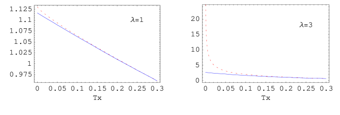
Figure 1: The dashed line is the l.h.s of (4.13) evaluated numerically and the solid line is the asymptotic expansion in the r.h.s, for two different values of $\lambda$.

The above procedure can be followed also for the $n\neq 0$ modes, for which the leading order term in the sum is $k=l=|n|$ (note that $n\neq 0$ implies $k\neq 0$ and hence $l\leq k<2k$). Expanding also to leading order in $\lambda^{2}/4\pi$ we get

$$h(i\omega_{n},p) \approx 2^{\lambda^{2}/2\pi}\lambda^{2}\left\{\frac{\delta_{n0}}{p^{2}+m_{T}^{2}}+\sum_{k\neq 0}\frac{\delta_{nk}}{p^{2}+\left[\left(\frac{\lambda^{2}+4\pi|k|}{2}\right)T\right]^{2}}\right\}$$ (4.14)

$$\approx 2^{\lambda^{2}/2\pi}\lambda^{2}\left\{\frac{\delta_{n0}}{p^{2}+m_{T}^{2}}+\sum_{k\neq 0}\frac{\delta_{nk}}{\omega_{k}^{2}}\right\},$$ (4.15)

where $\omega_{k}=2\pi kT$.

An important remark is in order here. The expressions (4.14) and (4.15) are equivalent in the DR limit. That is, they differ in ${\cal O}(p^{2}/(2\pi T)^{2})$, ${\cal O}(m_{T}^{2}/(2\pi T)^{2})$, ${\cal O}(\lambda^{2}/4\pi)$ terms. However, that does not mean that their analytic continuations to real energies will be equally close for all energies. For that reason we have given them separately because they provide a clear example of how the analytic continuation of slightly varying imaginary-time results (including arbitrary non-leading order terms) can give different physical answers. As a matter of fact, and for reasons to become clear below, we will also introduce a further modification of (4.15):

$$h(i\omega_{n},p)\approx 2^{\lambda^{2}/2\pi}\lambda^{2}\left\{\frac{\delta_{n0}}{p^{2}+m_{T}^{2}}\left(\frac{p^{2}+m_{s}^{2}}{m_{s}^{2}}\right)^{\lambda^{2}/4\pi}+\sum_{k\neq 0}\frac{\delta_{nk}}{\omega_{k}^{2}}\left(\frac{\omega_{k}^{2}}{m_{s}^{2}}\right)^{\lambda^{2}/4\pi}\right\}+{\cal O}\left[\frac{\lambda^{2}}{4\pi}\log\left(\frac{\lambda^{2}}{4\pi}\right)\right],$$ (4.16)

where $m_{s}={\cal O}(m_{T})={\cal O}(\lambda^{2}T)$ is a soft scale mass. We could take $m_{s}=m_{T}$, although (4.16) allows for more general situations (see below).

Finally, combining our results in this section with those in section 3.1, we get a high-$T$ expression for the slope of the MT charge density at the origin simply by replacing in (3.37) the coefficient $a_{1}$ of the $p^{2}$ term in $\Sigma_{T}(0,p)$, which we readily obtain from the zero mode contribution (4.11). The expression thus obtained is consistent with the result found in [13] for the charge density.

4.3 Analytic continuation to real energies

We now have an expression for the SG imaginary-time propagator $\Delta_{T}(i\omega_{n},p)$ based on $h(i\omega_{n},p)$ of (4.14)-(4.16). However, all the physical information we will need for dynamical quantities such as the conductivity is encoded in the retarded SG propagator at real energies. So one needs to analytically continue from the values $\Delta_{T}(i\omega_{n},p)$ at discrete imaginary frequencies $i\omega_{n}$ to arbitrary complex $\omega$.

The work of Baym and Mermin [30] showed, as explained in appendix A, that by enforcing a particular set of conditions, those given in (A.20), one produces a generalised propagator, $\Delta(\omega_{n},p)$, a function of complex energies $\omega$, whose values at $\omega=E\pm i\epsilon$ with $E$ real, give the retarded and advanced propagators, e.g, eq.(A.15).

Let us try to apply the procedure of Baym and Mermin to our expression (3.21) for the IT propagator, and try to find the retarded equivalent of (3.21). The generalised propagator will have the form

$$\Delta(\omega,p) = \Delta^{0}(\omega,p)+i\Sigma(\omega,p)\left[\Delta^{0}(\omega,p)\right]^{2}.$$ (4.17)

The analytic continuation of the first term in (3.21), a free IT propagator, is well known and used as an example in Appendix A and in section 2.1. The generalised continued function $\Sigma(\omega,p)$ can either be defined from (4.17) as the second term in the full propagator divided (truncated) by two generalised free propagators, $\Delta^{0}$. With a little work one can see that $\Sigma$ is indeed the analytic continuation of the IT function $\Sigma_{T}$, satisfying a slightly altered set of BM conditions (A.20) as its large energy behaviour can be such that $\Sigma\omega^{-4}$ vanishes for large $|\omega|$. It is then a short step from this generalised function to the retarded version using (A.15), and we will find the form

$$\Delta_{R}(E,p)=\Delta_{R}^{0}(E,p)+i\Sigma_{R}(E,p)\left[\Delta_{R}^{0}(E,p)\right]^{2},$$ (4.18)

where the first term is simply the free retarded propagator

$$\Delta_{R}^{0}(E,p)=\frac{i}{(E+i\epsilon)^{2}-p^{2}-\mu_{0}^{2}},$$ (4.19)

and the second term we can write as a retarded function multiplied by two free retarded propagators. Physically, we will be interested only in the small $p$ behaviour of $\Sigma(\omega,p)$ at high temperatures.

4.3.1 Approximate analytic continuations

In the previous sections, we have analysed the IT propagator to leading order in the high $T$ expansion (4.2). In fact, to that order, and according to (3.23), $\Sigma_{T}\approx-\Pi_{T}$, with $\Sigma_{T}$ in (4.3) and $\Pi_{T}$ the imaginary-time self-energy. One must bear in mind though that the analytic continuation of perturbative approximations to (3.23) for arbitrary complex energies must be done carefully, taking into account the poles of the free propagator and the $\Sigma$ functions. We will discuss this issue in section 4.3.3 below.

We have been able to find approximate expressions for $h(i\omega_{n},p)$ in the DR limit in (4.14)-(4.16). However, as discussed in greater generality in Appendix A, it is possible to find different functions whose analytic continuations all give the same IT result approximately, i.e. up to non-leading order terms in the DR limit. In this section, we will give explicit examples of such functions for the case of $h(i\omega_{n},p)$. All of them satisfy the conditions explained in Appendix A, i.e, such functions $h(\omega,p)$ are analytic off the real axis, $h\omega^{-4}$ vanish for large $|\omega|$ and $h(\omega=i\omega_{n},p)$ coincides with (4.14)-(4.16) to leading order in DR. In section 4.3.2, we will show that additional conditions may be imposed to ensure that the analytic continuation gives unique and meaningful physical answers. Let us then consider the following cases:

1. The first choice we could make is to neglect everything but the zero mode contribution in (4.14)-(4.16), which is dominant in DR with respect to the $n\neq 0$ modes, i.e, we take just $h(i\omega_{n},p)=h(0,p)\delta_{n0}$. As discussed in Appendix A (see (A.24) and (A.25)), analytic continuation gives a function $h_{1}(\omega,p)$ which vanishes everywhere off the real axis. Therefore, for $E\in\mathbb{R}$,

   $$h_{1R}(E,p)=h_{1}(E+i\epsilon)=0,$$ (4.20)

   so that only the constant term $h(0,0)$ would survive in the analytically continued retarded propagator of (4.3). In this regard, we note that when only the leading zero mode contribution is taken, i.e, when one replaces just $\left[Q^{2}(x,\tau)\right]^{-\lambda^{2}/4\pi}$ by $2^{\lambda^{2}/2\pi}e^{-\lambda^{2}T|x|/2}$ in (4.7), one can obtain closed expressions for the full self-energy sum in (3.24)-(3.25) up to ${\cal O}(p^{2})$ for any $\omega_{n}$, in terms of the Coulomb gas pressure and charge density, following similar steps as in [13]. However, as the example of the free propagator in Appendix A shows, this analytically continued propagator may be a very bad approximation (we will be more precise below). More realistic dynamics requires knowledge of the contribution of the $n\neq 0$ modes as well, even if each heavy mode is of a smaller order in our approximations than those neglected in calculating our zero mode contribution.

2. With this in mind, for the second case we take (4.14) as the starting point. From this form, one can apply the BM conditions (A.20) and derive a unique analytic continuation to real energies. In this case, as so often, a straight $i\omega_{n}\rightarrow\omega$ replacement in the functional form is essentially sufficient and we find

   $$h_{2}(\omega,p)=\frac{2^{\lambda^{2}/2\pi}\lambda^{2}}{p^{2}+\left[m_{T}-is\omega\right]^{2}}, s:=\theta\left[\mbox{Im}(\omega)\right]-\theta\left[-\mbox{Im}(\omega)\right]$$ (4.21)

   Note that the because of the modulus on the integer $k$ in (4.14), the form of the generalised function changes in the upper and lower half planes. This is common and through (A.15), this then corresponds to the retarded and advanced functions being distinct. Thus, the retarded function of (4.21) for real $E$ is $h_{2R}(E,p)=h_{2}(E+i\epsilon)$ with $s=1$. We remark that the result (4.21) obeys the BM conditions (A.20), reproducing all the Matsubara modes in (4.14) including $n=0$ (see the discussion in Appendix A).

3. If we take (4.15) instead of (4.14) as our IT function, then we would have, as our analytic continuation,

   $$h_{3}(\omega,p)=\frac{-2^{\lambda^{2}/2\pi}\lambda^{2}}{\omega^{2}-p^{2}-m_{T}^{2}},$$ (4.22)

   which again gives $h_{3}(\omega,p)\approx h(i\omega_{n},p)$ up to non-leading order terms in DR.

4. Finally, consider the fourth expression, obtained by analytically continuing (4.16):

   $$h_{4}(\omega,p)=-\lambda^{2}\left(\frac{2}{m_{s}}\right)^{\lambda^{2}/2\pi}\frac{\left(p^{2}+m_{s}^{2}-\omega^{2}\right)^{\lambda^{2}/4\pi}}{\omega^{2}-p^{2}-m_{T}^{2}}.$$ (4.23)

Clearly, we could obtain infinite variety in our analytic continuations just by modifying the original high-$T$ imaginary time expression by non-leading terms. The important point, as emphasized in Appendix A, is that the difference in physical quantities obtained by analytically continuing functions differing at non-leading order should be also of non-leading order. The four examples we have shown above are enough to show that this is not necessarily the case, unless further restrictions are applied, as we will see below. In fact, note that the analytic structure of the retarded version of those functions is very different. For instance, while $h_{2}$ in (4.21) for $s=1$ has complex single poles at $\omega=\pm p-im_{T}$, $h_{3}$ in (4.22) has real poles at $\omega=\pm E_{p}$ with $E_{p}=\sqrt{p^{2}+m_{T}^{2}}$ and $h_{4}$ in (4.23) has branch cuts for real $\omega^{2}>p^{2}+m_{s}^{2}$ in addition to the singular behaviour at $\omega^{2}=E_{p}^{2}$. In general, it is not difficult to realise that by moving the pole of the AC function in the complex plane by soft amounts, but preserving the zero mode contribution, the IT values at $n\neq 0$ remain unchanged to leading order. This can be easily achieved by replacing for instance $\left[\omega^{2}-p^{2}-m_{T}^{2}\right]$ by $\left[\omega^{2}-p^{2}-m_{T}^{2}+\omega M_{+}(\omega,p)\right]$ for $\mbox{Im}\omega>0$ in the denominator of $h$, with $M_{+}\ll 2\pi T$ a regular complex soft function such as the denominator does not vanish for $\mbox{Im}\omega>0$ and so on for $\mbox{Im}\omega<0$ with another function $M_{-}(\omega)$. Thus, while the $\omega=i\omega_{n}$ values are approximately equal, the contributions near the respective poles are arbitrarily different. The poles of the retarded propagator are related to physical modes at $T\neq 0$, or quasi-particles, while the branch cuts of the self-energy have to do with their decay rate. However, as it is clear from the previous discussion, we cannot determine the presence of soft poles unambiguously. There is no novelty in this as a general problem. For example, the whole programme of Padé approximants is based on how best to exploit such ambiguities. We will address this question again in section 4.3.3 although in the end the physical results will not be affected by our ignorance about the precise analytic structure.

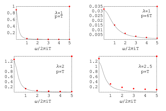
Figure 2: The solid line is $h_{3}(\omega,p)$ as given by (4.22) and the dots represent the IT values at $\omega=i\omega_{n}$ calculated numerically from the definition (4.4), for $n\leq 5$.

Before proceeding, let us comment that one can check numerically that the above functions indeed match the Matsubara modes approximately. For instance, in Figure 2 we have plotted the discrete $n$-values against the function $h_{3}(\omega,p)$ in (4.22). We see that the agreement is quite good, given the numerical uncertainties, for small $p$ and small $\lambda$, as expected. It gets worse as $\lambda$ or $p$ increase, although it still gives a reasonable agreement for $p\lesssim 2\pi T$. Note that as $p$ increases, the $n\neq 0$ mode become of the same importance as the zero mode, but the magnitude of the latter becomes much smaller. Recall that if we plotted the approximation (4.20), it would be just a function that vanishes everywhere except at the origin, where it matches the zero mode. From Figure 2 we see that this is a cruder approximation than $h_{3}$ in the range $\omega^{2}<(2\pi T)^{2}$. This gives support to the idea, explained in Appendix A, that we need to combine the information about the $n\neq 0$ modes, essential for AC, with that on the one soft mode $n=0$, even if we can only do this approximately.

4.3.2 A physical condition

We are interested in the fermion conductivity, which as we have seen is related to the SG retarded propagator. In particular, as we will see in section 5 (see eq.(5.2)) the time evolution of the conductivity is directly related to the Fourier transform of the retarded propagator:

$$\Delta_{R}(t,p)=\int_{-\infty}^{\infty}\frac{dE}{2\pi}e^{-iEt}\Delta_{R}(E,p),$$ (4.24)

$\Delta_{R}$ being given in (4.18), where in the high $T$ limit,

$$\Sigma_{R}(E,p)\approx\frac{\lambda^{2}}{2}m^{2}T^{2}\left(\frac{m^{2}}{T^{2}}\right)^{1-\lambda^{2}/4\pi}\tilde{h}_{R}(E,p),$$ (4.25)

with

$$\tilde{h}_{R}(E,p)=h_{R}(E,p)-h(0,0),$$

where $h(0,0)\approx 2^{\lambda^{2}/2\pi}\lambda^{2}/m_{T}^{2}$ to leading order.

Consider now the contribution of the second term, i.e the $\Sigma_{R}$ term, to (4.24). As discussed in Appendix A, the retarded function $\tilde{h}_{R}(z,p)$ can be also analytically continued to complex $z$, simply starting from the retarded $h_{R}(E,p)$ for real $E$ and replacing $E$ by $z$. This function, by construction, has its poles and branch cuts in the lower half plane. On the other hand, the generalized analytic functions $h$ we have been discussing in the previous sections satisfy Schwartz’s reflection principle $h(z^{*})=h^{*}(z)$ and the property $h(z)=h(-z)$. This means that $h_{R}(-z,p)=h_{R}^{*}(z^{*},p)$.

Therefore, taking $t>0$ and closing the integration contour from below the real axis, we find the following contribution to $\Delta_{R}(t,p)$ given by the poles at $\omega^{2}=\omega_{p}^{2}\equiv p^{2}+\mu_{0}^{2}$:

$$\frac{1}{2\pi}\frac{\partial}{\partial\mu_{0}^{2}}\left\{\frac{-2\pi i}{2\omega_{p}}\left[\tilde{h}_{R}(\omega_{p},p)e^{-i\omega_{p}t}-h_{R}(-\omega_{p},p)e^{i\omega_{p}t}\right]\right\}_{\mu_{0}^{2}=0}$$

$$=\frac{\partial}{\partial\mu_{0}^{2}}\frac{1}{\omega_{p}}\left\{\mbox{Im}\left[\tilde{h}_{R}(\omega_{p},p)e^{-i\omega_{p}t}\right]\right\}_{\mu_{0}^{2}=0}$$

$$=\frac{1}{2p^{3}}\left[\mbox{Re}\tilde{h}_{R}(p,p)\left(\sin pt-pt\cos pt\right)-\mbox{Im}\tilde{h}_{R}(p,p)\left(\cos pt-pt\sin pt\right)\right]$$

$$-\frac{1}{2p^{2}}\left(\mbox{Re}\tilde{h}_{R}^{\prime}(p,p)\sin pt-\mbox{Im}\tilde{h}_{R}^{\prime}(p,p)\cos pt\right),$$ (4.26)

where $\tilde{h}_{R}^{\prime}=(\partial/\partial\omega)\tilde{h}_{R}(\omega,p)$. Note that $\tilde{h}_{R}$ does not depend on $\mu_{0}$ (see our comments about the IR behaviour in section 3) and that the expression (4.26) is real, as it should, since it contributes to the conductivity. Therefore, from (4.26) we see that $\Delta_{R}(t,p)$ has a term growing linearly in time (and so does the conductivity) unless $\tilde{h}_{R}(p,p)=0$ (although $\tilde{h}_{R}^{\prime}(p,p)$ will be in general different from zero).

Hence, if we want the conductivity to remain bounded in time, as seems physically reasonable this gives us the following condition for the retarded $\Sigma$ function on the mass shell of the SG massless field:

$$\Sigma_{R}(E^{2}=p^{2},p)=0$$ (4.27)

for $\epsilon\rightarrow 0^{+}$. This is an extra, physical, condition, in addition to the BM mathematical ones discussed in Appendix A.

From the IR behaviour of $h_{R}$ as $p\rightarrow 0^{+}$, discussed in previous sections, it is not difficult to see that once we demand (4.27), the rest of the contributions in (4.26) remain bounded in time when taking the Fourier transform also in the $p$ variable. As for the contributions of the poles of $\tilde{h}_{R}$ in the lower half plane, say at $\omega=\pm E(p)-i\gamma(p)$ with $\gamma(p)\geq 0$, their contribution is damped at long time as $\exp(-\gamma t)$ if $\gamma\neq 0$ (as it is the case for instance for the retarded version of (4.21) where $\gamma=m_{T}$) and one can check that for $\gamma=0$, although there is no exponential damping, the contributions to $\Delta_{R}(t,p)$ remain bounded as well, since one gets $\sin Et$ and $\cos Et$ instead of $\sin\omega_{p}t$ and $\cos\omega_{p}t$ as in (4.26), so that all the $\mu_{0}$ dependence is in the $t$-independent contributions.

Finally, if $h_{R}(z,p)$ has also a branch cut, as it is the case for $h_{4R}(z,p)=h_{4}(z+i\epsilon,p)$ with $h_{4}$ in (4.23) for $z=-i\epsilon\pm E^{\prime}$ with $E^{\prime}>\sqrt{p^{2}+m_{s}^{2}}$, the branch cut contribution to $\Delta_{R}(t,p)$ gives also a bounded contribution, as long as $h_{R}(E,p)$ is integrable for $E\geq E_{cut}$ where $E_{cut}$ is the cut endpoint. For instance, for the case of $h_{4R}$ with $m_{s}=m_{T}$, such a contribution is proportional to

$$\int_{E_{p}}^{\infty}dE\frac{1}{(E^{2}-p^{2})^{2}}\frac{\sin(Et)}{(E^{2}-E_{p}^{2})^{1-\frac{\lambda^{2}}{4\pi}}},$$

with $E_{p}=\sqrt{p^{2}+m_{T}^{2}}$, which is perfectly finite and bounded in time, since the integrand behaves like $(E-E_{p})^{-r}$ with $0<r<1$ near $E_{p}$. The same is true for $m_{s}\neq m_{T}$, as it is discussed in section 5, see eq. (5.11).

Of the four cases considered in the previous section, only $h_{3}$ and $h_{4}$ satisfy the on-shell condition (4.27) and they yield respectively:

$$\Sigma_{3R}(E,p) \approx -\mu_{T}^{2}\frac{(E+i\epsilon)^{2}-p^{2}}{(E+i\epsilon)^{2}-p^{2}-m_{T}^{2}},$$

$${}\Sigma_{4R}(E,p) \approx -\mu_{T}^{2}\left[\frac{m_{T}^{2}m_{s}^{-\lambda^{2}/2\pi}\left[p^{2}+m_{s}^{2}-(E+i\epsilon)^{2}\right]^{\lambda^{2}/4\pi}}{(E+i\epsilon)^{2}-p^{2}-m_{T}^{2}}+1\right],$$

with

$$\mu_{T}^{2}=2^{1+\lambda^{2}/2\pi}m^{2}\left(\frac{m^{2}}{T^{2}}\right)^{1-\lambda^{2}/4\pi}.$$ (4.28)

Note that $\mu_{T}^{2}\ll m^{2}$ in DR, but we have not made any assumption about the relation between $m$ and $m_{T}$ and therefore between $\mu_{T}$ and $m_{T}$. However, it is natural to take $m$ and $m_{T}$ of the same order, since both are soft scales much smaller than $T$, and therefore $\mu_{T}^{2}\ll m_{T}^{2}$ . In fact, most of our results below will be expressed as corrections of order $\mu_{T}^{2}/m_{T}^{2}$. This means that the temperatures should be at least as high as $T\raise 1.29167pt\hbox{$>$\kern-7.5pt\lower 4.30554pt\hbox{$\sim$}}m/\lambda^{2}$ but they can be even much higher, which would have simply the effect of making the perturbative corrections much smaller.

4.3.3 Analytic structure and quasi-particles

Here, we will discuss some relevant features of the retarded propagators we have just obtained. The poles of the retarded propagator in the lower half plane give the dispersion law for quasi-particles in the thermal bath [17], which are the dual SG bosons in this context. In moving from the MT model, with two fundamental degrees of freedom, to the sine-Gordon model with one bosonic degree of freedom, we appear to have lost a degree of freedom. However, the second bosonic degree of freedom was trivial and was integrated out when exploiting the duality [15]. For instance, for $m/T\rightarrow 0$, bosonic and fermionic modes both contribute the same amount to the free energy in 1+1 dimensions. We must take account of this trivial bosonic mode in the thermodynamic quantities, but for dynamic quantities, only the single SG mode is necessary for equivalence with the two massive Thirring modes.

On the other hand, the branch cuts of the self-energy $\Pi(E,p)$ along the real axis correspond to the decay rates of those quasi-particles and the corresponding discontinuity $\Pi(E+i\epsilon)-\Pi(E-i\epsilon)=2i\mbox{Im}\Pi$ across the cuts can in principle be calculated by cutting the self-energy diagrams. Cutting rules and discontinuities in the self-energy at finite temperature have been extensively analysed in the literature [31, 32, 33]. To one loop in perturbation theory [31] and for the case of a single particle with mass $m$, the self-energy has branch cuts at $s=4m^{2},9m^{2},\dots$ ($s=E^{2}-p^{2}$) corresponding to the decay into two-particle, three-particle states and so on. These are the $T=0$ cuts although the discontinuity across the cuts is $T$-dependent. New ”thermal” cuts may appear, even to one loop, corresponding to processes of emission and absorption of particles in the thermal bath, not allowed at $T=0$.

In our case, even to leading order in the high $T$ limit, we are dealing with a nonperturbative resumation of diagrams in the coupling constant $\lambda$, as for instance in (4.4). As commented above, this is essential in order to obtain a meaningful IR behaviour for physical quantities such as the transport coefficients and it has forced us to use analytic continuations to approximate imaginary-time results. Thus, we do not have a clear interpretation in terms of Feynman diagrams that can be cut and therefore we do not know a priori what should be the analytic structure of the self-energy on the real axis. To make matters worse, and as emphasized in previous sections, with our DR approximation we cannot determine the position of the self-energy branch points or the poles of the retarded propagator. One can move the poles by soft amounts (i.e, of ${\cal O}(m_{T})$) and the analytic continuation will still match the IT values to leading order in the DR high-$T$ limit.

The point we want to make here is that, despite this apparent limitation, we can give meaningful physical predictions. The key point is that, once the extra condition (4.27) is imposed, the errors produced by changing the poles or the branch cuts are perturbatively small. We will check this explicitly in section 5. Before that, let us discuss in some more detail the analytic structure of the AC propagators. First, let us define the retarded self-energy in terms of the retarded propagator as customary,

$$\Delta_{R}(\omega,p)=\frac{i}{(\omega+i\epsilon)^{2}-p^{2}-\Pi_{R}(\omega,p)}.$$ (4.29)

Note that we cannot write (4.18) as $\Delta_{R}\sim i(\omega^{2}-p^{2}+\Sigma_{R})^{-1}$ since, as explained in section 3, we do not get an infinite series of $\Sigma$ insertions. Remember also that the poles of $\Delta_{R}(\omega,p)$ lie in the lower half of the complex plane $\omega$ and the retarded propagator for real energies $E$ is $\Delta_{R}(E,p)$.

Consider first (4.21), which gives for $\mu_{0}=0$

$$\Delta_{2R}(\omega,p)=i\frac{\mu_{T}^{2}\left[s+2i(\omega+i\epsilon)m_{T}\right]+s\left[s-m_{T}^{2}+2i(\omega+i\epsilon)m_{T}\right]}{s^{2}\left[s-m_{T}^{2}+2i(\omega+i\epsilon)m_{T}\right]},$$ (4.30)

where $s=(\omega+i\epsilon)^{2}-p^{2}$ and $\mu_{T}^{2}$ defined in (4.28).

We see that $\Delta_{2R}$ has a double pole at $s=0$ and single poles at $\omega=\pm p-im_{T}$. On the other hand, the retarded self-energy defined through (4.29) satisfies $\mbox{Im}\Pi_{R}(E+i\epsilon,p)\neq 0$ for any $E$ real different from zero, so that it has a cut along the whole real axis. Note also that $\Pi_{R}(\omega,p)$ is singular for the complex $\omega$ solution of $\mu_{T}^{2}\left[s+2i(\omega+i\epsilon)m_{T}\right]+s\left[s-m_{T}^{2}+2i(\omega+i\epsilon)m_{T}\right]=0$.

We compare this with the solution (4.22), which gives

$$\Delta_{3R}(\omega,p)=i\frac{s+\mu_{T}^{2}-m_{T}^{2}}{s\left[s-m_{T}^{2}\right]}.$$ (4.31)

Now, $\Delta_{3R}$ has single (and real) poles at $s=0$ and $s=m_{T}^{2}$ and the self-energy is real on the real axis except at the singular point $(\omega+i\epsilon)^{2}=p^{2}+m_{T}^{2}-\mu_{T}^{2}$.

The analytic structure of the above two solutions is completely different. As we have discussed already, the position of the poles and branch cuts change within DR. A different story though is the physical interpretation of the above results. First, note that the two solutions above for the retarded propagator have a common feature: the self-energy is singular close to the new ”thermal” poles (i.e, those different from $s=0$). That is, the distance between the singular points and the ”thermal” poles in the $\omega$ plane is proportional to $\mu_{T}$, which is much smaller than the positions of the poles themselves, which is ${\cal O}(m_{T})$. The values for which the self-energy diverges are related to pinching or end point singularities [33] and it is therefore not clear that those poles should be interpreted as quasi-particles energies or damping rates. However, the behaviour of the two above solutions near the pole at $s=0$ is very different. Thus, while $\Delta_{3R}(s\rightarrow 0)\sim i(1-\mu_{T}^{2}/m_{T}^{2})s^{-1}$ is a massless pole with a $T$-dependent residue, $\Delta_{2R}(s\rightarrow 0)\sim i(\pm 2ip\mu_{T}^{2})/(\pm 2ip-m_{T})s^{-2}$ is a double pole. A double pole is an indication of the breakdown of the Schwinger-Dyson expansion around the massless propagator [33] and in fact we have seen in the previous section that it leads to unphysical behaviour. Note that the condition (4.27), which is satisfied by $\Delta_{3R}$ but not by $\Delta_{2R}$, ensures that the pole at $s=0$ is a single pole. Therefore, our physically acceptable solution for the retarded propagator is consistent with a massless dispersion law. However, we want to make clear that our approach does not allow to say whether the quasi-particles dispersion law really remains massless or there is a ”thermal” true pole of ${\cal O}(m_{T})$ as it happens in the HTL approach. All that we can say is that $m_{T}$ plays the role of a screening mass in the sense explained in previous sections. In addition, note that the contribution to physical observables from the pole of $\Delta_{3R}$ at $s=m_{T}^{2}$ is reduced by a $(\mu_{T}^{2}/m_{T}^{2})$ factor with respect to that of the $s=0$ pole, so that the thermal contributions in DR are always perturbatively small with respect to the leading order. Another indication of the ambiguities in the interpretation of the retarded propagator is the result (4.23), which also satisfies the condition (4.27) and we could have chosen to have a branch cut starting at $m_{s}=2m_{T}$, as expected from a true thermal quasi-particle pole of mass $m_{T}$ [33].

Summarizing, the DR approach does not allow us to fix uniquely the position of poles and branch cuts of the retarded propagator. Although the results suggest the appearance of a thermal mass scale $m_{T}$, it is not clear within our approximation scheme whether this is the mass of the quasi-particles. Thus we see that the double-lined ”propagator” introduced in section 3 really has a pole but this does not simply correspond to a stable particle of mass $m_{T}$. The important point is that the physics we are interested in, i.e, the conductivity, does not depend on our choice of functions to be continued analytically, once the physical condition (4.27) is imposed. For instance, taking (4.22) or (4.23) will produce the same answer, to the order we are considering here.

5 Physical applications. The conductivity.

Transport coefficients are usually discussed in Fourier space and the expressions such as (2.11) for conductivity, used to motivate the calculations of the full scalar propagator, were in energy and momentum. Our interest is in the DC conductivity, i.e. the $\omega,p\rightarrow 0$ limit of (2.11). However, the free field propagators $\Delta_{0}$ appearing in expressions such as (2.11) are poorly defined in this limit because they are massless. The DC conductivity then seems to depend on how the $\omega,p\rightarrow 0$ limit is approached although, in simple cases, as in (2.16), there may not be any difficulty in making a choice. For more complicated expressions more care is needed. Such unsatisfactory behaviour is well known in thermal field theory for zero-momentum Green functions [18, 19], often coming from Landau damping cuts across zero energy rather than a massless pole as here.

Our solution is to remain in coordinate space where one can specify a realistic experimental situation, with systems of finite size examined for finite times. The lack of analyticity found at zero momentum and energy at finite temperature can be associated with space-time causality. After all, $\delta j$ should be zero if we are looking at a point that is space-like separated from a non-zero electric field. The usual formulae will then give $\sigma=0$. On the other hand for the same problem at a time-like separated point, $\sigma$ will be non-zero. Likewise a simple implementation of a DC conductivity measurement, the $E,p\rightarrow 0$ limit, implies that a constant electric field has been applied for all times. If the system has finite correlation times, this may be an acceptable approximation to an experiment where the fields were set up a ‘long time’ before. However, the presence of poles or cuts, at zero energy and momentum, suggests that there are long time scales in the problem, so one can not simply assume that such a DC current can be switched on adiabatically in the distant past. In practice, working in time and space is not especially difficult, and it is much more physical, so it greatly simplifies the physical interpretation of real-time calculations in finite temperature problems.

Turning to our model, we must first specify the electric field. From Gauss’ law the electric field due to a single charge in vacuo is constant in size, merely switching sign at the location of the charge, i.e. $E\propto q(\theta(x-x_{1})-\theta(x_{1}-x))$ is the field due to single static charge at $x_{1}$. A constant field over a finite region $x_{1}$ to $x_{2}$ comes from having two charges of opposite signs at $x_{1}$ and $x_{2}$. Thus we choose

$$E_{cl}(t,x)=\bar{E}\theta(t-t_{0})\left[\theta(x-x_{1})-\theta(x-x_{2})\right],$$ (5.1)

where $\bar{E}$ is a constant and $x_{2}>x_{1}$ for simplicity, so that $E=\bar{E}$ if $x_{1}<x<x_{2}$, and is zero otherwise. This is then a close analogue of the usual large parallel plate capacitor problem encountered in 3+1 electrostatics.

However, we are turning on the field suddenly, so the two charges appear instantaneously at time $t_{0}$. The field is switched on over a region which is not initially time-like separated, so we must be careful later with the interpretation. This means that we have to calculate

$$\delta j^{(1)}(X) = i\frac{\lambda^{2}}{4\pi^{2}}\bar{E}\int_{t_{0}}^{\infty}dt^{\prime}\int_{x_{1}}^{x_{2}}dx^{\prime}\;\int\frac{d^{2}p}{(2\pi)^{2}}e^{-ip_{0}(t-t^{\prime})}e^{ip(x-x^{\prime})}.(-ip_{0})\Delta_{R}(p_{0},p)$$ (5.2)

$$= \frac{\lambda^{2}}{4\pi^{2}}\bar{E}\sum_{j=1,2}s_{j}\int\frac{d^{2}p}{(2\pi)^{2}}e^{-ip_{0}(t-t_{0})}e^{ip(x-x_{j})}\frac{\Delta_{R}(p_{0},p)}{p},$$

where $s_{1}=+1$, $s_{2}=-1$ and $X\equiv(x,t)$.

As shown in section 4, the full retarded propagator is made up of two parts, as given in (4.18). The first part is the free contribution and for the second one we have obtained explicit expressions in the DR high-$T$ limit. Let us analyse those two contributions separately.

5.1 Free boson term

Consider the first term, the single free propagator (4.19) and its contribution $\delta j_{a}^{(1)}(X)$ to the total $\delta j^{(1)}(X)$. This gives, for $t\geq t_{0}$:

$$\delta j_{a}^{(1)}(X) = \frac{\lambda^{2}}{2\pi^{2}}\bar{E}\sum_{j=1,2}s_{j}\int_{0}^{\infty}\frac{dp}{2\pi}\frac{\sin\left[p(x-x_{j})\right]}{p}\frac{\sin(\omega_{p}(t-t_{0}))}{\omega_{p}}$$ (5.3)

$$= \frac{\lambda^{2}}{8\pi^{2}}\bar{E}\sum_{j=1,2}s_{j}\left[(t-t_{0})(\theta_{2}^{j}-\theta_{3}^{j})+(x-x_{j})\theta_{1}^{j}\right].$$

where $\omega_{p}=\sqrt{p^{2}+\mu_{0}^{2}}$ and in the second line we have taken the $\mu_{0}\rightarrow 0^{+}$ limit after performing the $p$ integral. This result is clearly IR and UV finite, even if $\mu_{0}\rightarrow 0^{+}$. However, it is also causal, i.e. the current is zero if its space-like separated from the electric field region. The regions where the $\theta$ functions are non-zero are shown in Figure 3. The $\theta_{1}^{j}$ is one in region I - the region inside the forward light cones from the point $(t_{0},x_{j})$, i.e. the space-time point where the charge at position $j$ was switched on. It is zero elsewhere. The $\theta_{2}^{j}$ is then one only in region II to the right (positive $x$) of this and $\theta_{3}^{j}$ is one in region III to the left (negative $x$). Each of the terms in the sum for $j$ represent the effects of switching on at $t_{0}$ the electric field of a single charge at $x_{j}$. Note that the regions II and III are space-like connected to $(t_{0},x_{j})$ yet the change in the current is non-zero in these regions. This is because we have actually switched on the electric field of these charges instantaneously, and the static field is non-zero everywhere. A more realistic experiment would be to switch on the charges slowly (charging up a parallel plate capacitor). However this behaviour is not important for the case at hand. In fact, when we add the two terms in the sum for $j$ together we get

$$\delta j^{(1)}_{a}(X) = j_{a,max}\left[\theta_{11}+2(t-t_{0})L^{-1}\theta_{23}+\left[(t-t_{0})-(x-x_{2})\right]L^{-1}\theta_{21}\right.$$ (5.4)

$$\left.+\left[(x-x_{1})+(t-t_{0})\right]L^{-1}\theta_{13}\right],$$

$$j_{a,max} = \frac{\lambda^{2}}{8\pi^{2}}\bar{E}L,$$ (5.5)

where

$$\theta_{kl}=\theta_{k}^{1}\theta_{l}^{2},\;\;\;L=x_{2}-x_{1}.$$ (5.6)

The regions where the $\theta_{kl}$ functions are non-zero are shown in Figure 4. If the distance between the charges is $L$, i.e. the electric field $\bar{E}$ is on over a region of length $L$, then the current profile rises until at time $t-t_{0}-L/2>0$ it reaches a state where there is a central region where the current saturates at $j_{a,max}$ and is proportional to $L$ for constant electric field strength $\bar{E}$. This region extend a length $t-t_{0}-L/2$ either side of the mid-point of the electric field region for $t>L$. The current profile then drops linearly to zero at a distance $t-t_{0}+L/2$ either side of the mid-point. Its then zero beyond this, as it must as these regions are not in causal contact with the region of electric field (i.e, the regions $22$ and $33$ in Figure 4). This is shown in Figure 5.

Thus there are two conclusions. After an initial rise time, the current in the region of electric field is constant proportional to $L$. Thus the contribution to the conductivity from the first term in the full propagator is

$$\sigma=\frac{\lambda^{2}L}{8\pi^{2}}.$$ (5.7)

as in (2.16). Thus the current is always proportional to the voltage, $\bar{E}L$, and independent of $L$ so the conductance (the inverse of the resistance) is constant, at $G=\lambda^{2}/8\pi^{2}$, as in (2.17), whatever the length of the material is studied! However, life is not quite so simple. Note that in fact the current is also nonzero outside the region of the electric field. In fact, the current is reaching the same constant level everywhere as fast as causality allows. This is nothing but the effect of the SG massless effective mode, propagating at the speed of light, since $dx/dt=1$ for the extreme points in Figure 5. Note also that the result (5.7) is consistent with our analysis in section 2.1, eq.(2.16). Let us study now the behaviour of the temperature corrections to this result in the DR, high-$T$ limit.

Figure 3: Light cone regions for single charge

Figure 4: Light cone regions for two charges

Figure 5: Current profile (first, free term), $t>t_{0}+L$

5.2 High-$T$ corrections

In section 4 we have discussed the DR high-$T$ (and large distances) approximation to the retarded propagator. Let us write the contribution of the second term in the r.h.s of (4.18) to the current in (5.2) as

$$\delta^{(1)}j_{b}(X) = -i\bar{E}\frac{\lambda^{2}}{4\pi^{2}}\mu_{T}^{2}\frac{\partial\Xi(X)}{\partial\mu_{0}^{2}},$$ (5.8)

with $\mu_{T}^{2}$ given in (4.28). Only the cases $h_{2}$ and $h_{4}$ of (4.21) and (4.23) satisfy the physical constraint (4.20). Taking them in turn, $h_{2}$ of (4.21) gives

$$\Xi(X) = \sum_{j=1,2}s_{j}\int\frac{d^{2}p}{(2\pi)^{2}}e^{-ip_{0}(t-t_{0})}e^{ip(x-x_{j})}\frac{1}{p}\frac{1}{(p_{0}+i\epsilon)^{2}-p^{2}-\mu_{0}^{2}}$$ (5.9)

$$\times \left[\frac{m_{T}^{2}}{p^{2}+m_{T}^{2}-(p_{0}+i\epsilon)^{2}}-1\right],$$

When the $p_{0}$ integral in (5.8) is evaluated by the Residue Theorem for $t\geq t_{0}$, there is a contribution coming from the poles at $p_{0}=\pm\omega_{p}-i\epsilon$ and another one from the poles at $p_{0}=-i\epsilon\pm\sqrt{p^{2}+m_{T}^{2}}$. The second one is always bounded. The remaining $p$-integrals can be expressed in terms of Bessel functions as

$$\delta^{(1)}j_{b}(X) = -\frac{\mu_{T}^{2}}{m_{T}^{2}}\left\{\delta j^{(1)}_{a}(X)\right.$$ (5.10)

$$- \frac{\lambda^{2}}{8\pi^{2}}\bar{E}\sum_{j=1,2}s_{j}\mbox{sgn}(x-x_{j})\left[\theta(t-|x-x_{j}|)\int_{0}^{|x-x_{j}|}duJ_{0}\left[m_{T}\sqrt{t^{2}-u^{2}}\right]\right.$$

$$+ \left.\left.\theta(|x-x_{j}|-t)\int_{0}^{t}duJ_{0}\left[m_{T}\sqrt{t^{2}-u^{2}}\right]\right]\right\}.$$

for $t_{0}=0$. The first term in the r.h.s of (5.10) renormalises the maximum value (5.5) for the free current. This is the effect of the renormalization of the residue of the free propagator discussed in section 4.3.3. As commented above, this gives rise to a current that in time-like regions rises to a constant independent of the length, i.e. a constant resistance. The second term in (5.10) is the effect of the ”massive” mode $m_{T}$, yielding a causal oscillatory behaviour that is bounded in time. Our results are shown in Figure 6.

Finally, let us discuss the result of the calculation using (4.23) for the analytic continuation of the propagator, which also satisfies the physical condition (4.27). Taking $m_{s}>m_{T}$ for definiteness, it is not difficult to see that the corresponding $\delta^{(1)}j_{b}$ has three contributions. The first one is the pole at $p_{0}^{2}=\omega_{p}^{2}$ which gives again a renormalization of the factor multiplying $\delta^{(1)}j_{a}$ which becomes $1-\mu_{T}^{2}/m_{T}^{2}+(\lambda^{2}/4\pi)\mu_{T}^{2}/m_{s}^{2}$ and therefore is of the same order as the first contribution in the r.h.s. of (5.10) (remember that $m_{s}$ and $m_{T}$ are of the same order and $\mu_{T}^{2}\ll m_{T}^{2}$) ). The second contribution comes from the poles at $p_{0}^{2}=p^{2}+m_{T}^{2}$ and gives exactly the same as the second and third terms in the r.h.s. of (5.10), multiplied by the factor $(1-m_{T}^{2}/m_{s}^{2})^{\lambda^{2}/4\pi}$. Finally, the third contribution is given by the cut for $p_{0}^{2}>p^{2}+m_{s}^{2}$ and gives

$$\left[\delta^{(1)}j_{b}\right]_{cut} = {\bar{E}}\frac{\lambda^{2}}{\pi^{3}}\sin(\lambda^{2}/4)\frac{\mu_{T}^{2}m_{T}^{2}}{m_{s}^{5}}\sum_{j=1,2}s_{j}\int_{0}^{\infty}dp\frac{\sin p(x^{\prime}-x^{\prime}_{j})}{p}$$ (5.11)

$$\times \int_{\sqrt{p^{2}+1}}^{\infty}dE\frac{\left(E^{2}-p^{2}-1\right)^{\lambda^{2}/4\pi}\sin Et^{\prime}}{(E^{2}-p^{2})^{2}\left(p^{2}-E^{2}+m_{T}^{2}/m_{s}^{2}\right)},$$

for $t_{0}=0$, where $t^{\prime}=m_{s}t$ and $x^{\prime}=m_{s}x$. This latter contribution, because of the $\sin(\lambda^{2}/4)$ factor, is negligible in the small $\lambda$ limit compared to the other two. We have checked the equivalence between the results obtained with these two representations of the propagator, numerically for several values of the parameters in the DR limit. Therefore, we confirm explicitly that the difference between the physical transport coefficients calculated with different versions of the analytically continued propagator is negligible within the DR limit, as long as the condition (4.27) is enforced.

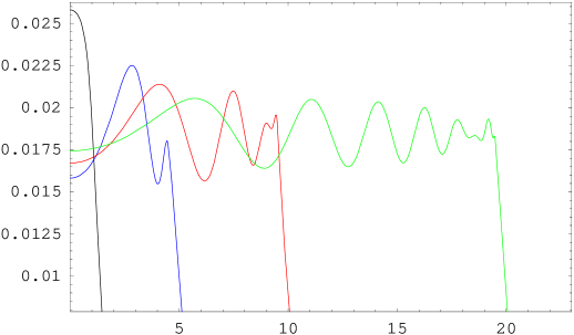
Figure 6: Time evolution of the second term $-\delta^{(1)}j_{b}(X)/j_{max}$. The horizontal axis is $mx$ and $T=5m$, $L=1/m$ and $\lambda=1$. The curves in each plot are for times $tm=1.5,5,10$ and $20$ with the later time plots extending further in $mx$.

The end result is that, once the transients have passed,

$$\delta j^{(1)}(X) = j_{max}\left[\theta_{11}+2(t-t_{0})L^{-1}\theta_{23}+\left[(t-t_{0})-(x-x_{2})\right]L^{-1}\theta_{21}\right.$$ (5.12)

$$\left.+\left[(x-x_{1})+(t-t_{0})\right]L^{-1}\theta_{13}\right]$$

where

$$j_{max}\approx\frac{\lambda^{2}}{8\pi^{2}}\bigg{(}1-\frac{\mu^{2}_{T}}{m^{2}_{T}}\bigg{)}{\bar{E}}L$$ (5.13)

with $\theta_{kl}=\theta_{k}^{1}\theta_{l}^{2}$ defined as before. For high enough temperature, $\mu_{T}^{2}\ll m_{T}^{2}$, and so the effect of the non-leading terms in the temperature expansion is relatively small. This describes the regime in which chiral symmetry is approximately restored (the ‘molecular phase’ of [13, 10, 12]) and for that reason gives results close to those of the massless Thirring model. This condition is satisfied in all our plots. At fixed temperature the effect increases as the fermionic coupling becomes strong.

In terms of the dual boson parameters the conductance $G$ of the fermion field is now

$$G\approx\frac{\lambda^{2}}{8\pi^{2}}\bigg{(}1-\frac{\mu^{2}_{T}}{m^{2}_{T}}\bigg{)}\approx\frac{\lambda^{2}}{8\pi^{2}}\bigg{(}1-\frac{2^{3+\lambda^{2}/2\pi}}{\lambda^{4}}\bigg{(}\frac{m^{2}}{T^{2}}\bigg{)}^{2-\lambda^{2}/4\pi}\bigg{)}$$ (5.14)

However, in terms of the fermionic mass $m$ and coupling constant $g^{2}$, as would follow from a diagrammatic description in terms of fermion loops, we find high temperature corrections to $G$ of (2.17) of the form

$$G\approx\frac{1}{2\pi(1+g^{2}/\pi)}\bigg{[}1-2^{(5\pi+3g^{2})/(\pi+g^{2})}\frac{(1+g^{2}/\pi)^{2}}{16\pi^{2}}\bigg{(}\frac{m^{2}}{T^{2}}\bigg{)}^{(\pi+2g^{2})/(\pi+g^{2})}\bigg{]}.$$ (5.15)

The next nonleading term is down by powers of $m/T$.

The power of duality in resumming series in $g^{2}$ that would be unobtainable otherwise is very striking, and is our main practical result.

6 Conclusions

We have analyzed the fermion conductivity at finite temperature in the massive Thirring/sine-Gordon (MT/SG) models. We have shown that the use of the dual degrees of freedom can avoid the usual problems associated with the infra-red behaviour of transport coefficients at finite temperature. In this case, the SG boson is the relevant quasi-particle mode in the limit of strong fermion coupling constant and the fermion conductivity can be related to the boson retarded propagator, which we have analyzed in detail.

First, we have studied the imaginary-time SG boson propagator. Its leading order for small momentum at zero frequency has been related to the MT fermion charge density. Particular attention has been paid to the high $T$ limit, for small boson coupling $\lambda$ (dimensional reduction). In this limit, a thermal scale $m_{T}=\lambda^{2}T/2$ emerges. This is the scale which screens the large distance behaviour of the propagator and therefore ensures that the results for the transport coefficients are well behaved in the IR limit. This is a common feature of high-$T$ expansions, where the $m_{T}$ scale comes from high-$T$ diagrams of arbitrarily higher order in the coupling constant. In this sense, our results provide a partial resummation in $\lambda$ which ensure the IR finiteness.

We have paid particular attention to the problem of the analytic continuation of the approximate (in DR) imaginary-time results. We have shown that by imposing the standard mathematical conditions to the propagator only, one cannot guarantee that the difference between analytically continued propagators of approximately equal imaginary-time propagators remains small. However, one can ensure that physical results remain insensitive to this choice by imposing extra physical conditions. In particular, we have shown this in detail for the conductivity, where we demand that it remains bounded in time. We have also discussed the role of the ”thermal” modes in the retarded propagator. Because of the ambiguities associated with the analytic continuation of approximate results, the position of poles and branch cuts in the retarded propagator cannot be determined with this approach. We have considered specific examples, where the analytic structure differs but the imaginary-time values are equivalent to leading order in DR. Our results are not in contradiction with considering $m_{T}$ a true thermal mass, but are also compatible with massless quasi-particles, since $m_{T}$ is a soft quantity. The crucial point is that none of these interpretations prohibits us obtaining physically meaningful results for the conductivity. However, on the formal side, it is disappointing that we have had to apply to many approximations in what is an “exactly solvable” model.

Once the physical condition is imposed, the fermion conductivity for this model can be studied perturbatively at high $T$. We have found that the resistance remains approximately constant for long times, inside the causality region. The free SG field contribution correspond to an exactly constant resistance, while the high $T$ corrections renormalize that constant and generate also bounded transient oscillations.

Thus, we have managed to study in detail several aspects of this problem which will be generic to more realistic problems where the imaginary-time formalism is used. In particular, we have highlighted the importance of the analytic continuation of approximate results and the IR zero Matsubara mode. Studies of analytic continuation for propagators [30] or higher-order Green functions [34] are usually made in terms of exact functional forms and do not depend on the values at zero Matsubara energies. As we have noted, the IR sector is of vital importance to the physics and the only direct piece of information in this sector is in fact the zero Matsubara mode, the one not used in determining the analytic continuation. We have therefore proposed an additional condition to be used in these cases, (A.30) which combined to physical conditions such as (4.27) allows us to find unambiguous physical predictions.

Appendix A Thermal propagators and Analytic Continuation

The standard analysis is given in several places, such as [17]. We repeat it here to fix our notation and definitions, but also because we wish to go beyond the usual discussions to see how best to deal with approximate results.

Take $t\in\mathbb{C}$, complex and lying on a given directed contour $C$ with ends separated by $-i\beta$. Define the thermal propagator as

$$\Delta_{C}(x,t)\equiv\langle\langle T_{C}\phi(x)\phi(0)\rangle\rangle\equiv\Delta^{>}(x,t)\theta_{C}(t)+\Delta^{<}(x,t)\theta_{C}(-t),$$ (A.1)

where $\Delta^{>}(x,t)=\langle\langle\phi(x)\phi(0)\rangle\rangle$, $\Delta^{<}(x,t)=\langle\langle\phi(0)\phi(x)\rangle\rangle$, and $\theta_{C}$ means time ordering along $C$ as usual. The KMS conditions are then

$$\Delta^{>}(x,t)=\Delta^{<}(x,t+i\beta).$$ (A.2)

The Fourier transforms of the propagators are defined to be

$$\Delta^{>}(x,t)=\int_{-\infty}^{+\infty}\frac{d\omega}{2\pi}\int_{-\infty}^{+\infty}\frac{dp}{2\pi}e^{-i\omega t}e^{ipx}\Delta^{>}(\omega,p),$$ (A.3)

and similarly for other propagators. Then, KMS conditions in momentum space read

$$\Delta^{<}(\omega,p)=e^{-\beta\omega}\Delta^{>}(\omega,p)$$ (A.4)

Now we introduce the spectral function

$$\rho(\omega,p)=\Delta^{>}(\omega,p)-\Delta^{<}(\omega,p)=\left(1-e^{-\beta\omega}\right)\Delta^{>}(\omega,p).$$ (A.5)

Note that in position space $\rho(x,t)=\langle\langle[\phi(x),\phi(0)]\rangle\rangle$. On the other hand, $\Delta^{>}(x,t)=\Delta^{<}(x,-t)$ so that $\rho(x,-t)=-\rho(x,t)$ and then $\rho(\omega,p)=-\rho(-\omega,p)$ so that

$$\int_{-\infty}^{\infty}\frac{d\omega^{\prime}}{2\pi}\rho(\omega^{\prime},p)=0.$$ (A.6)

All versions of the propagator can be obtained from the spectral function. For instance, from (A.5) one readily has

$$\Delta^{>}(\omega,p) = \rho(\omega,p)\left[1+f(\omega)\right],$$

$$\Delta^{<}(\omega,p) = \rho(\omega,p)f(\omega),$$ (A.7)

where

$$f(x)=\frac{1}{e^{\beta x}-1}$$ (A.8)

is the Bose-Einstein distribution. The simplest example is that of a free scalar field of mass $m$, for which

$$\rho_{0}(\omega,p)=2\pi\epsilon(\omega)\delta(\omega^{2}-p^{2}-m^{2}).$$ (A.9)

More generally, let us introduce now the retarded and advanced propagators

$$\Delta_{R}(x-x^{\prime},t-t^{\prime}) = \theta(t-t^{\prime})\langle\langle[\phi(x,t),\phi(x^{\prime},t^{\prime})]\rangle\rangle$$ (A.10)

$$\Delta_{A}(x-x^{\prime},t-t^{\prime}) = \theta(t^{\prime}-t)\langle\langle[\phi(x^{\prime},t^{\prime}),\phi(x,t)]\rangle\rangle$$ (A.11)

which we define for real time $t-t^{\prime}$ only because of the non-analytic nature of the Heaviside functions.

Using the representation for the step function

$$\theta(t)=i\int_{-\infty}^{\infty}\frac{d\omega^{\prime}}{2\pi}\frac{e^{-i\omega^{\prime}t}}{\omega^{\prime}+i\epsilon}$$ (A.12)

with $\epsilon\rightarrow 0^{+}$, the retarded propagator can also be written in terms of the spectral function as

$$\Delta_{R}(\omega,p)=i\int_{-\infty}^{\infty}\frac{d\omega^{\prime}}{2\pi}\frac{\rho(\omega^{\prime},p)}{\omega-\omega^{\prime}+i\epsilon}.$$ (A.13)

Now unlike the retarded function in real-time with its Heaviside functions, this energy-dependent retarded function has a simple extension into the complex energy plane. It is convenient to define a general function of complex energy

$$\Delta(z,p)=-\int_{-\infty}^{\infty}\frac{d\omega^{\prime}}{2\pi}\frac{\rho(\omega^{\prime},p)}{z-\omega^{\prime}}.$$ (A.14)

This seems a little trivial as it simply related to both retarded and advanced functions through

$$\Delta_{R}(\omega,p) = -i\Delta(\omega+i\epsilon,p)$$

$$\Delta_{A}(\omega,p) = i\Delta(\omega-i\epsilon,p).$$ (A.15)

with $\omega\in\mathbb{R}$. The point is that, on assuming that the grand canonical average ensures uniform convergence [34] of the thermal traces, we are assured that this generalised propagator function $\Delta(z,p)$ is bounded and analytic for all complex energies $z$ except for real $z$, and $\Delta$ must tend to zero as $|z|\rightarrow\infty$ [30, 34]. These are properties we will exploit below so $\Delta$ is a useful intermediate object to work with.

Finally, let us introduce the imaginary time propagator $\Delta_{T}\equiv\Delta_{C}$ when $C\equiv[0,-i\beta]$. Then, changing variables to $\tau=it\in[0,\beta]\subset\mathbb{R}$ gives

$$\Delta_{T}(x,\tau)=\Delta^{>}(x,-i\tau)=\int_{-\infty}^{+\infty}\frac{d\omega}{2\pi}\int_{-\infty}^{+\infty}\frac{dp}{2\pi}e^{-\omega\tau}e^{ipx}\rho(\omega,p)(1+f(\omega)).$$ (A.16)

Therefore, the Fourier transform of the IT propagator

$$\Delta_{T}(i\omega_{n},p)=\int_{0}^{\beta}d\tau\int_{-\infty}^{\infty}dxe^{-ipx}e^{i\omega_{n}\tau}\Delta_{T}(x,\tau)$$ (A.17)

with $\omega_{n}=2\pi n/\beta$, reads, from (A.16),

$$\Delta_{T}(i\omega_{n},p)=-\int_{-\infty}^{\infty}\frac{d\omega^{\prime}}{2\pi}\frac{\rho(\omega^{\prime},p)}{i\omega_{n}-\omega^{\prime}}.$$ (A.18)

It is crucial that we remember that in energy coordinates, the IT propagator is a sequence of functions of $p$ and not actually a differentiable function of a continuous energy variable. This subtlety is easily missed since it is clear that we can relate the generalised propagator function, $\Delta$, to the IT propagator through

$$\Delta(z=i\omega_{n},p) = \Delta_{T}(i\omega_{n},p),\;\;\;n\in\mathbb{Z}$$ (A.19)

The key to analytic continuation is to note that we can not do the reverse easily, i.e. from the IT propagator we can not use this relationship alone to determine the full generalised propagator $\Delta$ at all complex energies. This is particularly confusing as analytic calculations, such as here, never give us a sequence of functions of $p$ for a calculation of the IT propagator. Instead, we write down a function of a continuous complex variable, $\omega_{n}$, and then note that for the IT propagator it is only to be taken at Matsubara energies. The obvious analytic continuation is to drop the restriction to Matsubara frequencies in such IT propagator expressions, and inspired by (A.19) we would guess that we have then found the generalised propagator $\Delta$. Unfortunately, this analytic continuation procedure is not unique as it stands. For instance, multiplying the IT propagator by arbitrary factors of $\exp(i\beta\omega_{n})=1$ would give different results for $\Delta$ but would not alter the values at Matsubara frequencies, so that (A.19) holds.

There is, however, a way forward and we can find a scheme for analytically continuing from the IT function that gives the unique function $\Delta$. The necessary and sufficient conditions were first stated by Baym and Mermin [30]. We simply quote here the result: given the IT discrete propagator $\Delta_{T}(i\omega_{n})$, then the unique function $\Delta(\omega)$ satisfies the following BM conditions:

$$1. \Delta(z=i\omega_{n})=\Delta_{T}(i\omega_{n}),\;\;\;|n|\in\mathbb{Z}^{+}$$

$${}2. \lim_{|z|=\infty}\left\{\Delta(z,p)\right\}=0\;\;\;\forall\;\mbox{Im}(z)\neq 0$$

$${}3. \Delta(z,p)\mbox{ is analytic }\;\;\forall\;\mbox{Im}(z)\neq 0,\pi$$ (A.20)

Therefore, if the result of an imaginary-time calculation can be written as $\Delta_{T}(z,p)$, analytic off the real axis and satisfying the second BM condition, it is then guaranteed to be the one generalised propagator function $\Delta(z,p)$.

The retarded and advanced functions for real energy are then given by (A.15), and a simple Fourier transform will then give the real-time retarded and advanced functions required for dynamical problems [17]. This is the usual situation when dealing with perturbative calculations, when the Matsubara sums in the loops are performed first [17]. However, the key point here is that we are dealing with nonperturbative expressions, like (4.4), which are nonperturbative in $\lambda$, so that this procedure is not valid and finding the appropriate analytic continuation of the original imaginary-time expression is not an easy task.

For instance, consider the free field case. The spectral function $\rho_{0}$ of (A.9), when inserted in (A.18), gives the sequence of functions

$$\Delta_{T}^{0}(i\omega_{n},p)=\frac{1}{\omega_{n}^{2}+p^{2}+m^{2}},\;\;\;n\in\mathbb{Z}$$ (A.21)

One quickly sees that the function

$$\Delta^{0}(z,p)=\frac{-1}{z^{2}-p^{2}-m^{2}}$$ (A.22)

obeys all the BM conditions (A.20) and therefore is the unique generalised propagator. The retarded propagator then follows from (A.15) as

$$\Delta_{R}^{0}(\omega,p)=\frac{i}{(\omega+i\epsilon)^{2}-p^{2}-m^{2}}.$$ (A.23)

This is temperature independent, as it should since the dispersion law for free particles does not depend on the medium properties.

A.1 Analytic continuation of approximate results

The results quoted above are all very well for a well defined function, such as the free propagator. However, in quantum field theory one does not have exact results for the Imaginary-Time Formalism (ITF) propagator at Matsubara frequencies. If we had been doing a numerical Monte Carlo calculation, the errors are partly statistical and random and partly come from the fact that only a finite number of Matsubara frequencies are calculated directly. This severely limits the accuracy of any possible analytic continuation from numerical data.

In an analytic calculation the errors are usually of a functional form, that is we assume that the approximate result differs from the true result by an amount given by a suitable analytic function. Indeed, we rarely calculate a sequence of numbers, but we invariably find a meromorphic functional form, even though we know it to be approximate and that it is strictly only valid for Matsubara frequencies. By checking that the function obeys the BM conditions (A.20), we are then guaranteed that we have already found the relevant AC of our approximate IT propagator to the whole complex plane and hence the approximate retarded propagator.

However, there is an interesting question one can ask. Suppose the functional error is order $\eta$ where $\eta$ may be a small coupling, a ratio of a mass scale to the high temperature, or whatever. Do the higher order, $O(\eta)$, corrections at the Matsubara frequencies also lead to small corrections to its analytic continuation for all complex energies? In our case are the functional corrections at Matsubara frequencies, when analytically continued, still small at real energies?

In fact the answer to this, posed in this simple minded way, is no. A small correction to the effective mass (real or complex) is a genuinely small change to the value of a propagator at all Matsubara frequencies. However, at real energies, near mass-shell, the propagator with and without the small shift will differ by large amounts. See our discussion in sections 4 and 5, or even the case of the free propagator analyzed below.

Luckily though, this example shows that we are not interested in reproducing the analytically continued form of the function such that the errors in the value of the function are always bounded. Our goal is that the physics obtained from such functions be well represented. Our functions are Green functions that are not directly physical, but tools used to calculate scattering rates etc. It is not important if our Green function differs by an infinite amount from the true function at some real energies, provided the physical predictions are accurate. For example, our experience tells us that any error in our knowledge of the exact value of a mass leads only to comparatively small errors in cross sections. What mattered to the physics was that the propagator always had a single pole that is important and a small shift in its position is going to be a small error in physical results. In our case, the conductivity will turn out to pick up small $O(\eta)$ errors even if these come from shifts in the mass value which leads to large differences in the propagators at certain values (near mass shell).

We have highlighted this example as this is the task we face in our model. Namely we calculate an exact ITF propagator but to produce more understandable expressions need to approximate it, in our case by expanding in $m/T$. We need to be sure that terms dropped at Matsubara frequencies do not alter the physics which depends on the appropriate analytic continuation, not simply on the values at Matsubara frequencies.

A.1.1 The free case.

To understand our approach, let us take the universal example of an exactly solvable quantum field theory, a free scalar field. We can compare the analytic continuation of approximations to the ITF version against the known exact result at real energies. Of course, in this case it seems a little stupid to make any approximation, such as DR, because we know the answer exactly. However, it will help us to see how we can be misled by DR.

The ITF propagator is given in (A.21). The unique generalised free propagator, the one obeying the BM conditions (A.20), is just (A.22). Suppose now that we were interested in the limit $\omega_{p}\ll 2\pi T$ where $\omega_{p}^{2}=p^{2}+m^{2}$ (large distances and inverse masses compared to $\beta$ or “soft, long wavelength” modes). This is what we will mean by high $T$ here (for the full interacting theory we will also take $T\gg m$, the fermion mass, see main text.). In that limit we find an approximate form for the propagator $\Delta_{1}$, much as one has in actual calculations. This is given by

$$\Delta_{T}^{0}(i\omega_{n},p)\approx\Delta^{0}_{T1}(i\omega_{n},p)\left[1+{\cal O}\left(\frac{\omega_{p}^{2}}{(2\pi T)^{2}}\right)\right],\;\;\;\Delta^{0}_{T1}(i\omega_{n},p):=\frac{\delta_{n0}}{\omega_{p}^{2}}$$ (A.24)

i.e., this is the DR approximation and we pick up only the zero mode ($n\neq 0$ represent “heavy” modes compared to $\omega_{p}$). Now, if we find the unique generalised propagator, $\Delta_{1}$, associated through (A.20) to the IT function $\Delta_{T1}$, this analytic continuation of the DR propagator $\Delta_{1}$ is

$$\Delta_{1}(\omega,p)=0\quad\mbox{for}\ \mbox{Im}\omega\neq 0,\pi\quad\Longrightarrow\quad\Delta_{1}^{R}(\omega,p)=\Delta_{1}^{A}(\omega,p)=0,$$ (A.25)

since it is the behaviour of the IT function near the limit point at $n=\pm\infty$ that controls the continuation, not the value at any one isolated finite $n$ Matsubara energies.

This is clearly not a very good approximation for the real-energy free propagator and is in fact inconsistent. First of all, we know that the true answer for the retarded propagator (A.23) is $T$-independent. Thus, if we continue first and then take the high $T$ limit, the answer is still (A.23). Therefore, the DR and analytic continuation operations do not commute in this case. Second, even though (A.24) is a good and well controlled approximation to the IT propagator at high $T$, that is not the case for its real-energy version in (A.25) when compared to the true answer in (A.23). For any arbitrarily small $\omega$, they differ by $\omega_{p}^{-2}$, which is not small at high $T$. On the other hand for $\omega>2\pi T$ the difference between the two is $\omega_{p}^{-2}\times{\cal O}\left(\omega_{p}^{2}/(2\pi T)^{2}\right)$ which is negligible to leading order in DR. Therefore, the conclusion is that by performing this DR style continuation, up to the accuracy of our approximations we are missing the right behaviour of the retarded propagator for frequencies $\omega\lesssim 2\pi T$.

Let us see if we can just solve the problem by making a better approximation. Consider $\Delta_{T2}$ where

$$\Delta_{T}^{0}(i\omega_{n},p) = \Delta_{T2}(i\omega_{n},p)\left[1+{\cal O}\left(\frac{\omega_{p}^{2}}{(2\pi T)^{2}}\right)\right],$$ (A.26)

$$\Delta_{T2}(i\omega_{n},p) = \frac{\delta_{n0}}{\omega_{p}^{2}}+\sum_{k\neq 0}\frac{\delta_{nk}}{(2\pi kT)^{2}}.$$ (A.27)

This is an improvement over the simple DR form of (A.24). Now all the modes appear as we take the leading high temperature term for each mode rather than working to a fixed accuracy for all terms. Notice however that the $n=0$ value does not fit the simple functional form we have given for the $n\neq 0$ heavy modes. Thus we should not be surprised when the unique analytic function obeying the BM conditions (A.20), when trying to match $\Delta_{T2}$, does not fit the $n=0$ term. The continuation is controlled purely by the analytic behaviour of the Matsubara sequence near the limit points of $\pm i\infty$, and here we find

$$\Delta_{2}(\omega,p)=-\frac{1}{\omega^{2}}.$$ (A.28)

The hard frequency behaviour is now a much better approximation to that of the exact answer, but it is still a bad approximation for the soft frequencies. This is not surprising as we have not used the one soft frequency value we know.

The problem does not lie in the mathematical process of analytic continuation. Both (A.25) and (A.28) satisfy the BM conditions (A.20) and they are therefore the unique continuations to the relevant generalised propagators of $\Delta_{T1}$ and $\Delta_{T2}$ respectively. On the other hand the same is true for the exact answer (A.23). Therefore, we have three apparently different continuations of the high temperature ITF propagator. This is not a contradiction, because we are dealing with approximate expressions for the IT propagator. Therefore, we are free to choose the continued version which gives a better approximation also for real frequencies. The problem is how can we specify the best continuation in a general case where we do not have the exact analytic answer? Is there any extra condition over and above those of Baym and Mermin (A.20) which we can demand?

The answer is that we should demand that the continuation also passes through the $n=0$ mode value, so incorporating the information about the $n=0$ mode. This value is unimportant for the continuations, since it is the behaviour of the ITF function near the limit points at $\pm i\infty$ which controls them. However, the $n=0$ value is the only direct information we have on the soft energy region, so we ought to use it if we expect to get that physics correct. However, the continuation is fixed uniquely by the value of the functions at hard Matsubara frequencies and so we can not just choose its value at zero energy. What we must do is exploit the fact that we are working with approximations and alter the hard frequency values by small amounts equivalent to the inherent errors of the approximation. We will do this until we have a set of values at Matsubara frequencies which give an analytic continuation which agrees up to the errors of the approximation scheme at all Matsubara frequencies with the known values, including the zero energy one.

Let’s see how this works for the free propagator. For that purpose we recognise that adding a small energy independent constant will do the trick, but there is no unique choice. In this case one can see from the functional form for the ITF propagator what the best choice is. Thus, adding ‘small’ corrections in a high temperature regime to the form $\Delta_{2}$, we find a third form

$$\Delta_{T}^{0}(i\omega_{n},p)=\Delta_{3}(i\omega_{n},p)\left[1+{\cal O}\left(\frac{\omega_{p}^{2}}{(2\pi T)^{2}}\right)\right],\;\;\;\Delta_{3}(i\omega_{n},p)=\frac{\delta_{n0}}{\omega_{p}^{2}}+\sum_{k\neq 0}\frac{\delta_{nk}}{(2\pi kT)^{2}+\omega_{p}^{2}}.$$ (A.29)

This is not a unique choice and here we have exploited the information in the ITF form. We therefore add a new condition for finding the unique generalised propagator through analytically continuing an IT propagator, namely

$$\Delta(i\omega_{n},p)\approx\Delta_{T}(i\omega_{n},p)\;\;\;\forall\;n\geq 0.$$ (A.30)

Note that this condition demands that $\Delta_{R}(0,p)=\Delta_{A}(0,p)$. However, this is guaranteed by the equal time commutation relations for two-point functions. An equivalent identity is true for higher-point functions [35].

In principle, all choices which differ by small amounts for each Matsubara value should give equivalent physical results, again up to the accuracy of the approximation scheme. However, as we have seen in section 4, in addition to the mathematical conditions we have just discussed, often one has to demand that the physical answer is meaningful. That is the case for the long-time behaviour of the conductivity discussed in section 5.

Appendix B Algebraic analysis of the sine-Gordon propagator

Here we will give more details about some of the calculations performed in section 3.

First, we will show how to arrive to (3.12). Using (3.1) with the SG generating functional given in [15] and taking the $\mu_{0}\rightarrow 0^{+}$ limit, we find

$$\Delta_{T}(x,\tau) = \Delta_{T}^{0}(x,\tau)+\frac{Z_{0}^{B}(T)}{Z_{SG}(T)}\sum_{n=1}^{\infty}\Gamma_{2n}(X_{1},\ldots,X_{2n})$$ (B.1)

$$\Gamma_{2n}(X_{1},\ldots,X_{2n}) = -\left(\frac{\lambda}{4\pi}\right)^{2}\left(\frac{1}{n!}\right)^{2}\left[\frac{\alpha}{2\lambda^{2}}\left(\frac{T}{\rho}\right)^{\lambda^{2}/4\pi}\right]^{2n}\left(\prod_{j=1}^{2n}\int_{0}^{\beta}d\tau_{j}\int_{-\infty}^{+\infty}dx_{j}\right),$$ (B.2)

$$\times \left[\sum_{l=1}^{2n}\ln\{[Q^{2}(x_{l},\tau_{l})]^{\epsilon_{l}\lambda/4\pi}\}\right]\left[\sum_{m=1}^{2n}\ln\{[Q^{2}(x_{m}-x,\tau_{m}-\tau)]^{\epsilon_{m}\lambda/4\pi}\}\right]$$

$$\times$$

$$\left(\prod_{j=2}^{2n}\prod_{k=1}^{j-1}\left[Q^{2}(x_{j}-x_{k},\tau_{j}-\tau_{k})\right]^{\epsilon_{j}\epsilon_{k}\lambda^{2}/4\pi}\right).$$

In order to obtain (3.12), we note that in the $l$ and $m$ sums in the above integral we can always relabel variables so that $x_{j}$ becomes any of the $x_{1},\dots,x_{n}$ if $j<n$ and so on for $x_{j}$ with $n<j<2n$. The term $\prod_{1\leq k<j\leq 2n}\left[Q^{2}(x_{j}-x_{k},\tau_{j}-\tau_{k})\right]^{\epsilon_{j}\epsilon_{k}\lambda^{2}/4\pi}$ remains invariant under such relabelling and also under the exchange $x_{j}\leftrightarrow x_{j+n}$, $\forall j=1,\dots,n$. In this way, we end up with (3.12), where the $\ln Q^{2}$ factors are written only in terms of $x_{1},x_{2}$ and $x_{2n}$.

Note that (B.2) is $\mu_{0}$ independent. For convenience, in (3.12) we have written the final expression in terms of $\Delta_{0}$ again. They are equivalent in the $\mu_{0}\rightarrow 0^{+}$ limit. Let us focus now on the UV behaviour of (B.2), i.e, small $x,\tau$. This corresponds to the behaviour of the integrand in near the regions where $Q^{2}\rightarrow 0^{+}$ in denominators and logs (see a similar discussion in [15] for the partition function). On the other hand, $Q^{2}(x,\tau)\approx\pi^{2}T^{2}(x^{2}+\tau^{2})$ for $(x,\tau)\rightarrow(0,0)$. Thus, clearly the most divergent contributions arise when $x=\tau=0$ and come from integrals like:

$$\int_{T,y\sim 0}d^{2}y\int_{T,y^{\prime}\sim y}d^{2}y^{\prime}\frac{1}{\left[Q^{2}(y-y^{\prime})\right]^{\lambda^{2}/4\pi}}\ln Q^{2}(y)\ln Q^{2}(y^{\prime})\approx\int_{r\sim 0}dr\frac{\ln^{2}r}{r^{[\lambda^{2}/2\pi-1}]},$$ (B.3)

where $\int_{T}d^{2}y\equiv\int_{0}^{\beta}dy_{0}\int_{-\infty}^{+\infty}dy_{1}$ and $r^{2}=y_{0}^{2}+y_{1}^{2}$. Clearly, the above integral converges near $r=0$ for $\lambda^{2}<4\pi$.

Next, we will give more details on the derivation of (3.25). When taking the Fourier transform of (B.2) we realise that the only dependence with $(\tau,x)$ appears in $\sum_{k=1}^{2n}\epsilon_{k}\ln Q^{2}(x_{k}-x,\tau_{k}-\tau)=-4\pi\sum_{k=1}^{2n}\epsilon_{k}\Delta_{T}^{0}(x_{k}-x,\tau_{k}-\tau)$, so that we can write (3.21) with

$$\Sigma_{T}(i\omega_{n},p)=\frac{\lambda^{2}}{4\pi}\frac{Z_{0}^{B}(T)}{Z_{SG}(T)}\sum_{n=1}^{\infty}\left(\frac{1}{n!}\right)^{2}\left[\frac{\alpha}{2\lambda^{2}}\left(\frac{T}{\rho}\right)^{\lambda^{2}/4\pi}\right]^{2n}\Sigma_{T}^{n}(i\omega_{n},p),$$ (B.4)

and

$$\Sigma_{T}^{n}(i\omega_{m},p)\Delta_{T}^{0}(i\omega_{m},p)=\prod_{j=1}^{2n}\int_{0}^{\beta}d\tau_{j}\int_{-\infty}^{+\infty}dx_{j}\prod_{1\leq k<j\leq 2n}\left[Q^{2}(x_{j}-x_{k},\tau_{j}-\tau_{k})\right]^{\epsilon_{j}\epsilon_{k}\lambda^{2}/4\pi}$$

$$\times\left[\sum_{j=1}^{2n}\epsilon_{j}\ln Q^{2}(x_{j},\tau_{j})\right]\left[\sum_{k=1}^{2n}\epsilon_{k}e^{i\omega_{m}\tau_{k}}e^{-ipx_{k}}\right].$$ (B.5)

Let us now write the expression (B.5) in a slightly different form, more convenient for our purposes. First, we relabel the variables in the $j$ and $k$ sums as we have just done with (B.2). Thus, separating the terms with $j=k$ and $j\neq k$ in the sum, we can write:

$$\left[\Sigma_{T}^{n}\Delta_{T}^{0}\right](i\omega_{m},p) = 2\prod_{j=1}^{2n}\int_{0}^{\beta}d\tau_{j}\int_{-\infty}^{+\infty}dx_{j}\prod_{1\leq k<j\leq 2n}\left[Q^{2}(x_{j}-x_{k},\tau_{j}-\tau_{k})\right]^{\epsilon_{j}\epsilon_{k}\lambda^{2}/4\pi}\ln Q^{2}(x_{1},\tau_{1})$$ (B.6)

$$\times \left\{ne^{i\omega_{m}\tau_{1}}e^{-ipx_{1}}+n(n-1)e^{i\omega_{m}\tau_{2}}e^{-ipx_{2}}-n^{2}e^{i\omega_{m}\tau_{2n}}e^{-ipx_{2n}}.\right\}$$

Now let us change variables to:

$$x^{\prime}_{2n}=x_{2n}-x_{2n-1},\ \dots,\ x^{\prime}_{2}=x_{2}-x_{1},\ x^{\prime}_{1}=x_{1},$$ (B.7)

so that

$$x_{j}=\sum_{l=1}^{j}x^{\prime}_{l}\quad,\quad x_{j}-x_{k}=\sum_{l=k+1}^{j}x^{\prime}_{l}\quad(k<j<2n),$$ (B.8)

and so on for $\tau^{\prime}_{2n},\dots\tau^{\prime}_{1}$. Note that with this change of variable,

$$\prod_{1\leq k<j\leq 2n}\left[Q^{2}(x_{j}-x_{k},\tau_{j}-\tau_{k})\right]^{\epsilon_{j}\epsilon_{k}\lambda^{2}/4\pi}=\prod_{1\leq k<j\leq 2n}\left[Q^{2}(\sum_{l=k+1}^{j}x^{\prime}_{l},\sum_{l=k+1}^{j}\tau^{\prime}_{l})\right]^{\epsilon_{j}\epsilon_{k}\lambda^{2}/4\pi}$$ (B.9)

is independent of $(x^{\prime}_{1},\tau^{\prime}_{1})$. This is just a consequence of two-dimensional translation invariance or, equivalently, total energy-momentum conservation in any diagram, which becomes manifest with this change of variables. Thus, we can separate the free propagator $\Delta_{T}^{0}(i\omega_{m},p)$ in the r.h.s of (B.6) yielding (3.25).

References

- [1] S.Jeon and L.G.Yaffe, Phys. Rev. D53 (1996) 5799.
- [2] S.Jeon, Phys. Rev. D52 (1995) 3591.
- [3] J.M. Luttinger, J. Math. Phys 4, (1963) 1154
- [4] F.D.M. Haldane, J. Phys C14 (1981) 2585.
- [5] S. Tomonaga, Prog. Theor. Phys.5 (1950) 544.
-
[6]
W. Apel and T.M. Rice, Phys. Rev. B26 (1982)7063;
C.L. Kane and M.P.A. Fisher, Phys. Rev. B46 (1992) 15233;
M.Ogata and H. Fukuyama, Phys. Rev. Lett. 73 (1994) 468. - [7] S. Tarucha, T. Honda, T. Saku, Sol. State Commun.94 (1995) 413.
- [8] D.L. Maslov and M. Stone Phys. Rev. B52 (1995) R5539.
- [9] D. Birmingham, I. Sachs, and S.N. Solodukhin, Conformal Field Theory Interpretation of Black Hole Quasi-normal Modes, hep-th/0112055.
- [10] K. Yoshida and W. Souma, Phys. Rev. D 64 (2001) 125002 [hep-th/0103075].
- [11] G. Parisi and N. Sourlas, Phys. Rev. Lett. 43 (1979) 744.
- [12] K. Yoshida, Phase Structure of Compact QED from the Sine-Gordon/Massive Thiring Duality, hep-th/0204086.
- [13] A.Gómez Nicola, R.J.Rivers and D.A.Steer, Nucl. Phys. B570 (2000) 475-505 [hep-th/9906236].
- [14] D.Delépine, R.González Felipe and J.Weyers, Phys. Lett. B419 (1998) 296.
- [15] A.Gómez Nicola and D.A.Steer, Nucl. Phys. B549 (1999) 409 [hep-ph/9810519].
- [16] J.I.Kapusta, Finite-Temperature Field Theory, Cambridge University Press, 1989.
- [17] M.Le Bellac, Thermal Field Theory, Cambridge University Press, 1996.
- [18] T.S.Evans, Z.Phys.C 36 (1987) 153-162.
- [19] T.S.Evans, Z.Phys.C 41 (1988) 333-339.
- [20] E.W. Fenton Phys. Rev. B46 (1992) 3754.
- [21] R.F.Alvarez-Estrada and A.Gómez Nicola, Phys. Rev. D57 (1998), 3618.
- [22] P.Ginsparg, Nucl. Phys. B170 (1980) 388.
- [23] T.Appelquist and R.D.Pisarski, Phys. Rev. D23 (1981) 2305.
- [24] K.Kajantie, M.Laine, K.Rummukainen and M.Shaposnikov, Nucl. Phys. B458 (1996) 90.
- [25] A.Lenard, J.Math.Phys.2 (1961) 682-693.
- [26] S.F.Edwards and A.Lenard, J.Math.Phys.3 (1962) 778-792.
- [27] R.D. Pisarski, Physica A158 (1989) 146; Phys.Rev.Lett. 63 (1989) 1129.
- [28] J.C.Taylor and S.M.Wong, Nucl.Phys.346 (1990) 115;
- [29] E. Braaten and R.D. Pisarski, Nucl. Phys. B337 (1990) 569; Phys. Rev. D42 (1990) R2156.
- [30] G.Baym and N.D.Mermin, J.Math.Phys.2 (1961) 232-234.
- [31] H.A.Weldon, Phys. Rev. D28 (1983) 2007.
- [32] R.L.Kobes and G.W.Semenoff, Nucl. Phys. B272 (1986) 329.
- [33] H.A.Weldon, Phys. Rev. D58 (1998) 105002 [hep-ph/0203057].
- [34] T.S.Evans, Nucl.Phys. B374 (1992) 340.
- [35] T.S. Evans, Nucl.Phys. B496 (1997) 486-502 [hep-ph/9504266].