$\theta$ dependence of SU($N$) gauge theories

Abstract:

We study the $\theta$ dependence of four-dimensional SU($N$) gauge theories, for $N\geq 3$ and in the large-$N$ limit. We use numerical simulations of the Wilson lattice formulation of gauge theories to compute the first few terms of the expansion of the ground-state energy $F(\theta)$ around $\theta=0$, $F(\theta)-F(0)=A_{2}\,\theta^{2}(1+b_{2}\theta^{2}+...)$. Our results support Witten’s conjecture: $F(\theta)-F(0)={\cal A}\,\theta^{2}+O(1/N)$ for sufficiently small values of $\theta$, $\theta<\pi$. Indeed we verify that the topological susceptibility has a nonzero large-$N$ limit $\chi_{\infty}=2{\cal A}$ with corrections of $O(1/N^{2})$, in substantial agreement with the Witten-Veneziano formula which relates $\chi_{\infty}$ to the $\eta^{\prime}$ mass. Furthermore, higher order terms in $\theta$ are suppressed; in particular, the $O(\theta^{4})$ term $b_{2}$ (related to the $\eta^{\prime}-\eta^{\prime}$ elastic scattering amplitude) turns out to be quite small: $b_{2}=-0.023(7)$ for $N=3$, and its absolute value decreases with increasing $N$, consistently with the expectation $b_{2}=O(1/N^{2})$.

1 Introduction

It is rather well established that four-dimensional SU($N$) gauge theories must have a nontrivial dependence on the angle $\theta$ that appears in the Euclidean Lagrangian as

$${\cal L}_{\theta}={1\over 4}F_{\mu\nu}^{a}(x)F_{\mu\nu}^{a}(x)-i\theta q(x)$$ (1)

where $q(x)$ is the topological charge density

$$q(x)={g^{2}\over 64\pi^{2}}\epsilon_{\mu\nu\rho\sigma}F_{\mu\nu}^{a}(x)F_{\rho\sigma}^{a}(x).$$ (2)

Indeed, the most plausible explanation of how the solution of the so-called U(1)_A problem can be compatible with the $1/N$ expansion (performed keeping $g^{2}N$ fixed [1]) suggests that in the pure gauge theory the ground-state energy depends on $\theta$ to leading order in $1/N$ [2]. Numerical nonperturbative studies, based on Monte Carlo simulations of the lattice formulation of SU($N$) gauge theories (see e.g. Ref. [3, 4] for recent reviews), have given nonzero estimates for the topological susceptibility $\chi$ at $\theta=0$, which is the zero-momentum two-point correlation function of $q(x)$, and therefore the second derivative of the ground state energy with respect to $\theta$ computed at $\theta=0$.

The $\theta$ dependence of the theory is described by the partition function

$$Z(\theta)=\int[dA]\exp\left(-\int d^{4}x{\cal L}_{\theta}\right)\equiv\exp[-VF(\theta)]$$ (3)

where $F(\theta)$ is the free energy (ground state energy) per unit space-time volume. Some information on the behavior of $F(\theta)$ comes from large-$N$ arguments. Witten argued [5] that in the large-$N$ limit $F(\theta)$ is a multibranched function of the type

$$F(\theta)=N^{2}{\rm min}_{k}\,H\left({\theta+2\pi k\over N}\right)$$ (4)

which is periodic in $\theta$, but not smooth since at some value of $\theta$ there is a jump between two different branches. More recently, the conjecture was refined [6] leading to a rather simple expression for $\Delta F(\theta)\equiv F(\theta)-F(0)$ in the large-$N$ limit, that is

$$\Delta F(\theta)={\cal A}\,{\rm min}_{k}\,(\theta+2\pi k)^{2}+O\left(1/N\right).$$ (5)

In particular, for sufficiently small values of $\theta$, i.e. $\theta<\pi$,

$$\Delta F(\theta)={\cal A}\,\theta^{2}+O\left(1/N\right).$$ (6)

Thus possible $O(\theta^{4})$ terms are expected to be depressed by powers of $1/N$. This conjecture has been supported using arguments based on a duality of large-$N$ gauge theories with string theory [6]. It has also been discussed in a field-theoretical framework in Ref. [7].

In this work we study the $\theta$ dependence of SU($N$) gauge theories, using numerical simulations of their Wilson lattice formulation. Numerical Monte Carlo studies of the $\theta$-dependence are made very difficult by the complex nature of the $\theta$ term. In fact the lattice action corresponding to the Lagrangian (1) cannot be directly simulated for $\theta\neq 0$, not to mention the difficulty to define a topological charge density on the lattice. Here we restrict ourselves to the region of small $\theta$ values, where one may expand $F(\theta)$ around $\theta=0$

$$\Delta F(\theta)=\sum_{i=1}A_{2i}\theta^{2i}.$$ (7)

The coefficient $A_{2}$ gives the topological susceptibility, i.e.

$$A_{2}={1\over 2}\chi,\qquad\chi\equiv\chi_{2}={1\over V}\langle Q^{2}\rangle_{\theta=0},$$ (8)

where $Q$ is the topological charge $Q=\int d^{4}x\,q(x)$. Higher order coefficients of the expansion (7) can be related to higher moments of the probability distribution $p(Q)$ of the topological charge. For instance,

$$A_{4}=-{1\over 24}\chi_{4},$$

$$\chi_{4}={1\over V}\left[\langle Q^{4}\rangle_{\theta=0}-3\left(\langle Q^{2}\rangle_{\theta=0}\right)^{2}\right].$$ (9)

A convenient parametrization of the free energy is achieved by introducing the dimensionless function

$$f(\theta)=\sigma^{-2}\,\Delta F(\theta),$$ (10)

where $\sigma$ is the string tension at $\theta=0$. The coefficients of the $\theta$-expansion of $f(\theta)$ are dimensionless scaling quantities. Let us write $f(\theta)$ in the form

$$f(\theta)={1\over 2}C\,\theta^{2}s(\theta)$$ (11)

where

$$C={2A_{2}\over\sigma^{2}}={\chi\over\sigma^{2}},$$ (12)

$$s(\theta)=1+b_{2}\theta^{2}+b_{4}\theta^{4}+...,$$ (13)

$$b_{2}={A_{4}\over A_{2}}=-{\chi_{4}\over 12\chi},$$ (14)

The function $s(\theta)$ parametrizes the corrections to a simple Gaussian behavior. Witten’s conjecture implies that $C$ has a finite nonzero large-$N$ limit $C_{\infty}$ with $O(1/N^{2})$ corrections, and $b_{2i}=O(1/N^{2})$. In particular one expects that $b_{2}$ is small, and that it should rapidly decrease with increasing $N$. We recall that the nonzero value of $\chi_{\infty}$ is essential to provide an explanation to the U(1)_A problem, and can be related to the $\eta^{\prime}$ mass [2, 8] through the relation

$$\chi_{\infty}=2{\cal A}={f_{\pi}^{2}m_{\eta^{\prime}}^{2}\over 4N_{f}}+O(1/N).$$ (15)

The quantity $b_{2}$ also lends itself to a physical interpretation, being related to the $\eta^{\prime}-\eta^{\prime}$ elastic scattering amplitude [8].

We present results for four-dimensional SU($N$) gauge theories with $N=3,4,6$. In particular, we determine the ratio $C=\chi/\sigma^{2}$ and the coefficient $b_{2}$ of the $O(\theta^{2})$ term in the function $s(\theta)$. Once verified that the results for $N=3,4,6$ are consistent with the expected behavior of the type $A+B/N^{2}$, the large-$N$ limit is determined by a fit. This allows us to obtain a rather accurate estimate of $C_{\infty}$. The estimated values of $b_{2}$ turn out to be very small, of the order of a few per cent, and appear to decrease rapidly with $N$, supporting Witten’s conjecture. Our results provide a first quantitative study of the function $s(\theta)$, cf. Eq. (11), related to the corrections to the $\theta^{2}$ term in the free energy $F(\theta)$, i.e. to a simple Gaussian behavior.

The paper is organized as follows. In Sec. 2 we describe the Monte Carlo simulations that we have performed. In Sec. 3 we present and discuss the results.

2 Numerical simulations

Table 1: Results of our Monte Carlo simulations for $N=3$. We tabulate the coupling $\beta$, the corresponding value of the string tension (taken from Ref. [9] for $N=3$), the lattice size $L$, the number of sweeps of the simulation $N_{\rm sw}$, the autocorrelation time $\tau_{Q}$ of the topological charge, the topological susceptibility $\chi$, the scaling ratio $C=\chi/\sigma^{2}$ and the coefficient $b_{2}$. The error on the ratio $C$ is computed by considering the errors on $\chi$ and $\sigma$ as independent.

$\beta$	$\sqrt{\sigma}$	$L$	$N_{\rm sw}/10^{6}$	$\tau_{Q}$	$10^{4}\,\chi$	$C$	$b_{2}$
$5.9$	0.2605(14)	$16$	8.7	29(1)	1.549(12)	0.0336(8)	$-$0.028(12)
		$12$	5.0		1.544(7)	0.0335(7)	$-$0.021(5)
$6.0$	0.2197(12)	$16$	6.4	77(5)	0.741(5)	0.0318(7)	$-$0.023(7)
		$12$	4.0	70(1)	0.728(5)	0.0312(7)	$-$0.032(3)
$6.1$	0.1876(12)	$16$	1.6	173(4)	0.382(6)	0.0308(9)	$-$0.032(9)
$6.2$	0.1601(10)	$20$	6.9	540(30)	0.1989(23)	0.0303(8)	$-$0.016(8)

Table 2: Results of our Monte Carlo simulations for $N=4$. We tabulate $\gamma\equiv\beta/(2N^{2})$, the corresponding value of the string tension (taken from Ref. [10]), the lattice size $L$ (in most cases we combine results obtained for $L^{4}$ and $L^{3}\times 2L$ lattices), the number of sweeps of the simulation $N_{\rm sw}$, the autocorrelation time $\tau_{Q}$ of the topological charge, the topological susceptibility $\chi$, the scaling ratio $C=\chi/\sigma^{2}$ and the coefficient $b_{2}$. The error on the ratio $C$ is computed by considering the errors on $\chi$ and $\sigma$ as independent.

$\gamma$	$\sqrt{\sigma}$	$L$	$N_{\rm sw}/10^{6}$	$\tau_{Q}$	$10^{4}\,\chi$	$C$	$b_{2}$
$0.335$	0.2959(14)	$12$	2.0		2.274(22)	0.0297(6)	$-$0.04(3)
$0.337$	0.2699(23)	$16$	2.3	85(4)	1.675(16)	0.0316(11)	$-$0.01(5)
$0.338$	0.2642(7)	$12$	7.9	105(4)	1.416(9)	0.0291(4)	$-$0.012(6)
$0.341$	0.2368(6)	$12$	6.4	207(6)	0.896(10)	0.0285(4)	$-$0.013(6)
$0.344$	0.2160(8)	$16$	6.8	410(20)	0.608(7)	0.0279(5)	$-$0.016(12)
		$12$	6.1	420(20)	0.595(18)	0.0273(9)	$-$0.019(7)
$0.347$	0.1981(5)	$16$	10.2	805(50)	0.425(10)	0.0276(7)	$-$0.011(8)

Table 3: Results of our Monte Carlo simulations for $N=6$. All tabulated quantities are as in Table 2.

$\gamma$	$\sqrt{\sigma}$	$L$	$N_{\rm sw}/10^{6}$	$\tau_{Q}$	$10^{4}\,\chi$	$C$
$0.342$	0.3239(8)	$12$	0.5	250(25)	2.55(7)	0.0232(7)
$0.344$	0.2973(5)	$12$	0.7	466(50)	1.79(6)	0.0228(8)
$0.348$	0.2535(6)	$16$	1.2	2675(500)	0.91(7)	0.0220(17)
		$12$	4.1	3080(120)	1.01(5)	0.0244(12)
		$10$	0.6		0.99(10)	0.0240(24)
$0.350$	0.2380(6)	$12$	0.5	$\gtrsim 3500$	0.76(9)	0.0237(28)

We consider the Wilson formulation of lattice gauge theories:

$$S=-N\beta\sum_{x,\mu>\nu}{\rm Tr}\left[U_{\mu}(x)U_{\nu}(x+\mu)U_{\mu}^{\dagger}(x+\nu)U_{\nu}^{\dagger}(x)+{\rm h.c.}\right],$$ (16)

where $U_{\mu}(x)\in$ SU($N$) are link variables. In our simulations we employed the Cabibbo-Marinari algorithm [11] to upgrade SU($N$) matrices by updating their SU(2) subgroups (we selected $N(N-1)/2$ subgroups and each matrix upgrading consists of $N(N-1)/2$ SU(2) updatings). This was done by alternating microcanonical over-relaxation and heat-bath steps, typically in a 4:1 ratio. Tables 1, 2 and 3 contain some information on our MC runs respectively for $N=3,4,6$: The coupling values $\beta$ or $\gamma\equiv\beta/(2N^{2})$, the corresponding value of the string tension (taken from Refs. [10, 9]), lattice sizes and the number of sweeps. The values of $\beta,\gamma$ were chosen to lie in the weak-coupling region, i.e., beyond the first order phase transition in the case $N=6$, and beyond the crossover region characterized by a peak of the specific heat for $N=3,4$; see Ref. [10] for a more detailed discussion of this point. Computing quantities related to topology using lattice simulation techniques is not a simple task. In a lattice theory the fields are defined on a discretized set, therefore the topological properties are strictly trivial. One relies on the fact that the physical topological properties are recovered in the continuum limit. Various techniques have been proposed and employed to associate a topological charge to a lattice configuration, see e.g. the review [3]. Here we employ a cooling technique. The topological charge has been measured on cooled configurations, using the standard twisted double plaquette operator. As is well known, the sum over the whole lattice of the twisted double plaquette, measured on cooled configurations, takes on values $Q_{t}\simeq k\alpha$, where $k$ is an integer and $\alpha\lesssim 1$. We determine the typical value of $\alpha$ by minimizing the average deviation of the twisted double plaquette from integer multiples of $\alpha$, and then assign to $Q$ the integer closest to $Q_{t}/\alpha$. This method eliminates the need for expensive, protracted cooling; usually fewer than 20 steps suffice (when using $N(N-1)/2$ subgroups) in order to observe a substantial convergence of the results, which become indistinguishable from results obtained using either improved operators for $Q$ or more cooling steps. We measured the topological charge $Q$ typically every 100 sweeps.

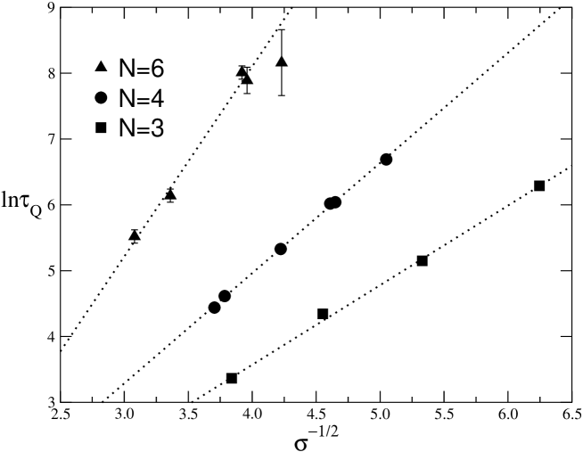
As already observed in Ref. [10], a severe form of critical slowing down affects the measurement of $Q$, posing a serious limitation for numerical studies of the topological properties in the continuum limit, especially at large values of $N$. In Tables 1, 2 and 3 we report the estimates of the autocorrelation time $\tau_{Q}$ obtained by a blocking analysis of the data, where the quoted errors on the estimates of $\tau_{Q}$ are just indicative, and attempt to quantify the uncertainty in extracting $\tau_{Q}$ from the blocking procedure outlined in Ref. [10]. These results are suggestive of an interesting phenomenon: As shown in Fig. 1, the data turn out to be well reproduced by an exponential behavior of the type

$$\ln\tau_{Q}\approx N\left(e_{N}\xi_{\sigma}+c_{N}\right)$$ (17)

where $\xi_{\sigma}$ is the length scale associated with the string tension, i.e. $\xi_{\sigma}\equiv\sigma^{-1/2}$, and $e_{N}$, $c_{N}$ are constants. A fit to the data for $N=3,4,6$, using the function (17), gives respectively $e_{3}=0.40(1)$ and $c_{3}=-0.42(4)$, $e_{4}=0.42(1)$ and $c_{4}=-0.43(4)$, $e_{6}=0.48(3)$ and $c_{6}=-0.55(9)$, showing that $\ln\tau_{Q}$ is approximately proportional to $N$ (at fixed $\xi_{\sigma}$). A qualitative explanation of this severe form of critical slowing down may be that topological modes give rise to sizeable free-energy barriers separating different regions of the configuration space. As a consequence, the evolution in the configuration space may present a long-time relaxation due to transitions between different topological charge sectors. We do not have a priori arguments in favor of the exponential behavior (17), which is just a guess arising naturally after observing the plot in Fig. 1. Note also that this dramatic effect is not observed in plaquette-plaquette or Polyakov line correlations, suggesting an approximate decoupling between topological modes and nontopological ones, such as those determining the confining properties.

Figure 1: The autocorrelation time $\tau_{Q}$ versus $\xi_{\sigma}\equiv\sigma^{-1/2}$. The dotted lines show the linear fits.

Figure 2: The scaling ratio $C=\chi/\sigma^{2}$ versus $\sigma$. The dotted lines show the linear fits.

3 Results

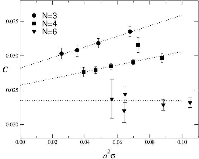
In this section we present and discuss the Monte Carlo results concerning the topological susceptibility $\chi$ and the function $s(\theta)$, cf. Eq. (11). In Tables 1, 2 and 3 we report $\chi$, the ratio $C=\chi/\sigma^{2}$, and the coefficient $b_{2}$, cf. Eq. (14). Data for different lattice sizes allow us to check for finite size effects: their comparison shows that they are under control. The ratio $C$ is plotted in Fig. 2 versus $\sigma$, to evidentiate possible scaling corrections, which are expected to be $O(a^{2})$ apart from logarithms. Such corrections are indeed clearly observed for $N=3$ and $N=4$, and one needs to allow for them in the fitting procedure to extrapolate to the continuum limit. For this purpose we assume a linear behavior

$$C=C_{\rm cont}+u\sigma,$$ (18)

which takes into account of the leading $O(a^{2})$ scaling correction and it is also supported by the data. We obtain

$$C_{\rm cont}=0.0282(12),\quad u=0.077(24)\qquad {\rm for}\quad N=3,$$ (19)

$$C_{\rm cont}=0.0257(10),\quad u=0.049(15)\qquad {\rm for}\quad N=4.$$ (20)

For $N=6$ no evidence of scaling corrections is observed. Therefore, in this case as final estimate we take the weighted average of the data for the largest values of $\beta,\gamma$, i.e. for $\gamma=0.348$ and lattice size $L=12,16$ and for $\gamma=0.350$, obtaining

$$C_{\rm cont}=0.0236(10)\qquad{\rm for}\quad N=6.$$ (21)

Results for smaller $\gamma$ are used to control scaling corrections: they are perfectly consistent, indicating that scaling corrections are at most of the size of the error .

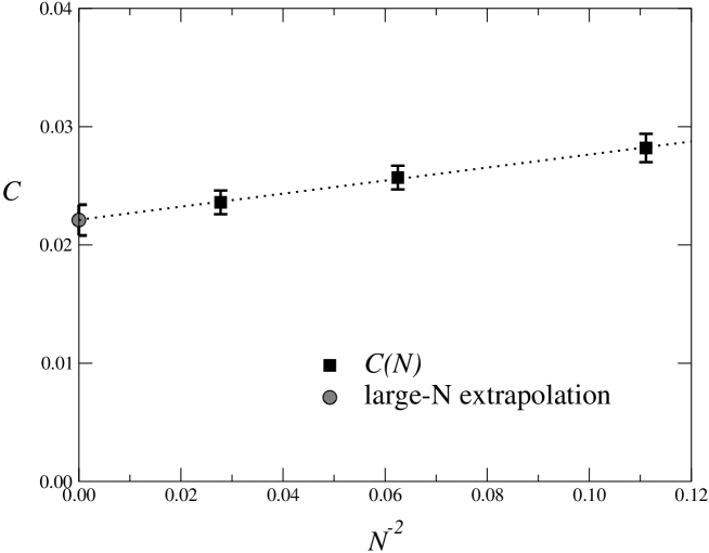
These results of $C_{\rm cont}$ are plotted in Fig. 3 versus $1/N^{2}$, which is the expected order of the asymptotic corrections in the large-$N$ limit. They are clearly consistent with a behavior of the type

$$C_{\rm cont}(N)=C_{\infty}+{B\over N^{2}}.$$ (22)

Assuming such a behavior, a fit to the results for $N=3,4,6$ gives

$$C_{\infty}=0.0221(14),\qquad B=0.055(18),$$ (23)

which provides a rather accurate estimate of the large-$N$ limit of $C$; this limit is clearly seen to be nonzero. Note that, extrapolating using only the $N=4,6$ results, we obtain a perfectly consistent result, i.e. $C_{\rm cont}=0.0219(20)$ and $B=0.06(4)$.

In order to compare with the numbers appearing in the literature, we translate the above results in physical units assuming the rather standard value $\sqrt{\sigma}=440\,{\rm MeV}$, for $N\geq 3$. We obtain $\chi_{\infty}^{1/4}=170(3)\,{\rm MeV}$, and $\chi^{1/4}=180(2)\,{\rm MeV}$ for $N=3$. These numbers have to be compared with the r.h.s. of Eq. (15), which, using the actual values of $f_{\pi}$, $m_{\eta^{\prime}}$, and $N_{f}=3$, gives $(191\,{\rm MeV})^{4}$; using the formula refined by Veneziano [8] for which $m_{\eta^{\prime}}^{2}\rightarrow m_{\eta^{\prime}}^{2}+m_{\eta}^{2}-2m_{K}^{2}$, one obtains $(180\,{\rm MeV})^{4}$. Our results for $N=3$ are in substantial agreement with the estimates obtained so far using various methods, see, e.g., Refs. [12, 13, 14, 15, 16, 17]. Ref. [9] presents an estimate of $C_{\infty}$ obtained by extrapolating results for $N=2,3,4,5$ using the formula (22); they obtain $C_{\infty}=0.0200(43)$ from $C_{\rm cont}(N=2)=0.0545(25)$, $C_{\rm cont}(N=3)=0.0355(33)$, $C_{\rm cont}(N=4)=0.0224(39)$ and $C_{\rm cont}(N=5)=0.0224(49)$. Our work improves these results essentially for two reasons: we performed simulations with much higher statistics, and we do not rely on $N=2$ data for our extrapolation, which may be too small a value of $N$. The large-$N$ extrapolation of Ref. [9] is in agreement with ours, although we note some differences in the finite $N$ results. The extrapolation of Ref. [9] strongly depends on the $N=2$ result, while their $N=2$ result is not fitted by our extrapolation (23), which would give approximately 0.036 for $N=2$. Thus, at this stage the agreement of the large-$N$ extrapolations appears to be rather accidental. The result for $N=2$ of Ref. [9] would suggest that $N=2$ is outside the region where the behavior (22) sets in.

Figure 3: The scaling ratio $C=\chi/\sigma^{2}$ versus $1/N^{2}$. The dotted line shows the linear fit to $A+B/N^{2}$.

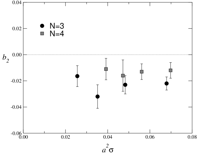
Let us now turn to the coefficient $b_{2}$ in the expansion (13) of the function $s(\theta)$, which determines the correction of $F(\theta)$ from the simple $\theta^{2}$ behavior. Note that a reasonably accurate computation of $\chi_{4}$, which is necessary to determine $b_{2}$, requires very high statistics due to a large cancellation between the two terms in its definition (9). Sufficiently accurate results have been obtained only in the cases $N=3,4$. The results are listed in Tables 1 and 2 for $N=3,4$ respectively. For $N=6$ they were always consistent with zero but with a large error, essentially due to the much smaller statistics available, taking also into account the critical slowing down phenomenon discussed before. We report only the most precise result obtained by a high-statistics simulation: $b_{2}=-0.01(2)$ for $\gamma=0.348$ and $L=12$. The results for $N=3$ and $N=4$ are plotted in Fig. 4. They show scaling within the errors. Assuming that the scaling corrections are negligible with respect to the typical errors of the data, as final estimate we consider the weighted average of the data, and as error we quote their typical error (in this computation we discard the data for $\beta=6.0$ and $L=12$ because of possible finite size effects). We obtain

$$b_{2}=-0.023(7),\qquad {\rm for}\quad N=3,$$ (24)

$$b_{2}=-0.013(7),\qquad {\rm for}\quad N=4.$$ (25)

For $N=6$ we report the estimate $b_{2}=-0.01(2)$ obtained at $\gamma=0.348$. These results show that $b_{2}$ is very small and are consistent with the hypothesis $b_{2}=O(1/N^{2})$. One may also assume $b_{2}\approx b_{2,2}/N^{2}$ and fit the above results, obtaining $b_{2,2}=-0.21(5)$.

Figure 4: The scaling ratio $b_{2}$ versus $\sigma$.

As already mentioned, we used a cooling technique to determine the topological charge of a lattice configuration. Several numerical studies have shown that cooling methods provide quite reliable results. Nevertheless, some of the arguments on which cooling relies are not rigorous. Therefore it would be worthwhile to confirm our results using alternative methods. A promising and more rigorous approach is the one based on the index theorem for Ginsparg-Wilson fermions [18, 19, 20], using, e.g., the overlap lattice fermion formulation [21].

In conclusion, we have computed the $\theta$ dependence of the ground-state energy of four-dimensional SU($N$) gauge theories around $\theta=0$, by evaluating numerically the coefficients of its expansion to $O(\theta^{4})$. We have verified that the coefficient of the $\theta^{2}$ term, which is the topological susceptibility, has a nonzero large-$N$ limit, in agreement with the picture proposed by Witten [2] to provide an explanation to the U(1)_A problem. Corrections to the leading $\theta^{2}$ term turn out to be very small. Indeed, the coefficient $b_{2}$ of the $\theta^{4}$ term is a few per cent for $N=3$, and appears to decrease with increasing $N$, consistently with Witten’s conjecture [6] implying $b_{2}=O(1/N^{2})$. Clearly, higher-order terms in the expansion in powers of $\theta^{2}$ might not be suppressed by powers of $N$ and therefore might spoil the simple $\theta^{2}$ behaviour predicted by Witten for large $N$. The study of these terms requires the measurement of higher moments of the topological charge probability distribution and are beyond the scope of this work. Thus, for $N\geq 3$ the simple Gaussian form

$$f(\theta)\approx{1\over 2}C\theta^{2}$$ (26)

is expected to provide a good approximation of the dependence on $\theta$ of the scaling free energy, up to $O(\theta^{6})$ terms, and therefore for a relatively large range of values of $\theta$.