Quantum Fields in a Big Crunch/Big Bang Spacetime

Abstract

We consider quantum field theory on a spacetime representing the Big Crunch/Big Bang transition postulated in ekpyrotic or cyclic cosmologies. We show via several independent methods that an essentially unique matching rule holds connecting the incoming state, in which a single extra dimension shrinks to zero, to the outgoing state in which it re-expands at the same rate. For free fields in our construction there is no particle production from the incoming adiabatic vacuum. When interactions are included the particle production for fixed external momentum is finite at tree level. We discuss a formal correspondence between our construction and quantum field theory on de Sitter spacetime.

I Introduction

Despite its overwhelming phenomenological success, the standard big bang cosmology is clearly incomplete. Its gaps and paradoxes provide some of the most powerful clues to fundamental theory that we possess. Indeed, it is increasingly evident that the real measure of success for string theory and M theory will be how well they face up to the challenges posed by cosmology. Perhaps the greatest challenge is that of describing the initial singularity, a moment of infinite density and curvature occurring some fifteen billion years ago in our past, a basic puzzle not resolved by cosmic inflation.

The initial singularity is often associated with the problem of the ‘beginning of time’. But the only thing one can legitimately infer from the existence of the singularity is that general relativity is incomplete. Rather than have time ‘begin’, which is a truly paradoxical notion, or to work with imaginary time formulations, it seems reasonable to explore the alternative possibility that time may be continued back through the singularity, and even arbitrarily far into the past. Such a view is consistent with what is known so far in string and M theory. Spatial geometry and topology are only approximate concepts, as evidenced by orbifold backgrounds[1], and allowed topology changing processes[2]. However, time is built in, in a fundamental role, and there is no evidence so far that it is allowed to ‘begin’ or ‘end’.

Recent attempts to construct cosmological scenarios employing ‘brane world’ constructions from M theory and string theory have led to a re-examination of these issues. The ‘ekpyrotic’ scenario[3], in which a brane collision is supposed to be the origin of the hot big bang, and its ‘cyclic’ version[4] in which such collisions occur periodically into the infinite past and future, provide alternate approaches to the classic cosmological puzzles conventionally addressed by inflation. In the cyclic model, the flatness, homogeneity and isotropy of today’s Universe is explained as a consequence of an epoch of vacuum energy domination in the previous cycle. And the density perturbations needed to seed structure formation were generated by an inter-brane attractive force near the end of the last cycle. An important precursor of these ideas was the ‘pre-big bang’ model of Veneziano et al.[5].

The ekpyrotic and cyclic models rest for the most part on conventional low energy effective field theory and gravity. One key event cannot be described within that approach, namely a collision between the two end-of-the-world boundary branes (or ‘orbifold planes’). In the four dimensional effective description this event appears to be unavoidable, since the four dimensional effective scale factor is initially contracting. The four dimensional fields appearing in the theory have positive (and growing) kinetic energy and this means, through the Friedman equation that the contraction cannot be reversed. Within a finite time one reaches a ‘big crunch’ singularity dominated by scalar kinetic energy, an event which appears at first sight to be irredeemably singular. From the the higher dimensional viewpoint the situation is more optimistic. The geometries of the branes are regular at the collision and the density of matter on the branes is finite. The five dimensional Riemannian curvature is finite everywhere away from the singular point. In fact, the only sense in which the higher dimensional geometry is singular is that the fifth dimension shrinks away to zero size[6].

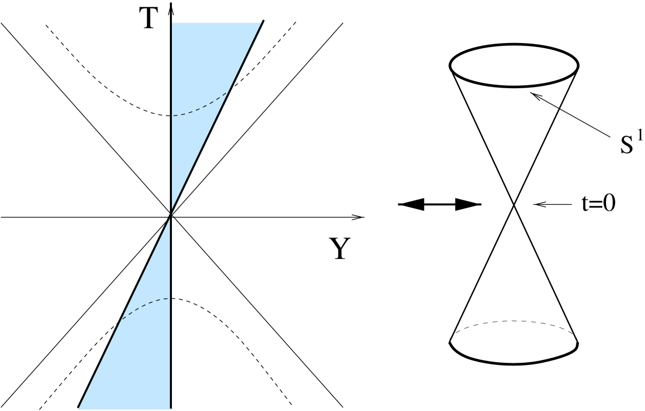
Figure 1: The compactified Milne universe. On the left is two dimensional Minkowski space. The Lorentz invariant coordinate $t$ satisfying $t^{2}=T^{2}-Y^{2}$ is constant on the dashed surfaces, which provide a spacelike foliation of the causal future and past of the origin. These surfaces are parameterized by a coordinate $y$. Identifying $y$ with $y+L$ compactifies space to produce the spacetime on the right, consisting of two Lorentzian cones joined tip-to-tip at $t=0$. If the circular sections of these cones are orbifolded by a $Z_{2}$, then the two fixed points of the $Z_{2}$ are two tensionless branes which collide and pass through one another at $t=0$.

It is crucial for the cyclic scenario, as currently formulated, that a satisfactory method be found for passing through the singularity corresponding to the collapse of the extra dimension. In particular, the issue of matching the density perturbations across this singularity has been a matter of fierce debate [7]. A matching rule was proposed in Ref.  References, according to which the growing mode scale invariant density perturbations developed in the pre-collapse phase are transmitted across the singularity. But it is also possible[7] to match in such a way that only the decaying mode is present in the final state. Interesting papers have subsequently appeared suggesting geometrical methods of regularizing the singularity[9], or employing scalar fields with a negative kinetic term to do so[10]. However, none of these methods yet yields a completely unambiguous result for the case of interest in the ekpyrotic or cyclic scenarios. We hope that the method developed here on more fundamental grounds, when extended to include gravitational backreaction, will be applicable to the cosmological case.

Ultimately this issue must be dealt with by string or M theory. Indeed, regardless of the ekpyrotic or cyclic scenarios, there are good reasons for believing that this type of singularity must be resolved if string theory is to make sense. The shrinking of the extra dimension can be accurately described using a slow motion (moduli space) approximation, which remains valid all the way to zero size. The low energy moduli of string theory and M theory are believed to be fundamental, more so even than the actions and Lagrangians they are derived from[12]. For example, these moduli are the parameters which interpolate from one corner of M theory to another. The shrinking away of one extra dimension, in finite time, seems to be perfectly allowed in string theory, either if it is one of the nine string theory dimensions[11], or if it is the tenth spatial dimension associated with M theory[6]. In the former case, the string coupling is constant and may be taken to be arbitrarily small, so stringy interactions should be negligible. In the latter case, the string coupling vanishes as the extra dimension shrinks away. Non-perturbative effects should, in this case, vanish even more rapidly than perturbative effects. Thus it is hard to see what would prevent this process. The question which must then be faced is: What happens next?

The moduli space description, and the higher dimensional picture, both lead to a natural continuation[6], illustrated in Figure 1. The extra dimension contracts to zero at a certain rate but immediately reappears at the same rate. In the brane picture, the two branes collide and pass through one another, a behaviour familiar from BPS solitons in other contexts. If the collision occurs at finite speed, one expects some associated particle production and consequent back-reaction.

In this paper, we take modest steps towards our eventual goal of a calculation of the consequences of a collision between boundary branes in M theory. There are significant technicalities to be faced even at the level of quantum fields, which is all that we shall discuss here. We shall propose a method of obtaining a unitary quantum field theory on the spacetime illustrated in Figure 1. Within free field theory, in our construction there is no particle production in passing from the big crunch to the big bang phase. However, once interactions are included, particle production occurs. For fixed external momenta, the particle production at the big crunch/big bang transition which is well defined and finite at tree level. It exhibits a power-law fall-off at high momenta which we argue would likely be replaced by exponential fall-off in string theory.

II Milne and Compactified Milne

The spacetime we are interested in is a subspace of $d+1$ dimensional Minkowski space, a trivial solution of $d+1$ dimensional general relativity or supergravity. The line element is

$$ds^{2}=-dT^{2}+dY^{2}+d\vec{x}^{2},$$ (1)

where we adopt units in which the speed of light is unity. We shall refer to $Y$ as the fifth coordinate, having in mind the picture that three of the $d-1$ coordinates $\vec{x}$ should provide the spatial dimensions of everyday existence, with the remainder compactified for example on a torus or orbifold. For example in eleven dimensional M theory, $d=10$ and six of the $\vec{x}$ dimensions would be taken to be compact.

The line element (1) may be rewritten in terms of new coordinates defined by $T=t\,{\rm cosh}(H_{5}y)$, $Y=t\,{\rm sinh}(H_{5}y)$, where $-\infty<t<\infty$ and $-\infty<y<\infty$ cover the causal future ($t>0$) and past ($t<0$) of the origin $Y=T=0$. We have here introduced the parameter $H_{5}$, with dimensions of inverse time. In these coordinates, (1) becomes

$$ds^{2}=-dt^{2}+H_{5}^{2}t^{2}dy^{2}+d\vec{x}^{2},\qquad-\infty<t<\infty,\quad-\infty<y<\infty.$$ (2)

The space comprising the causal future and past of the origin, and its light cone $T=\pm Y$ is what we shall define to be the Milne universe ${\cal M}$. The complement of ${\cal M}$ in Minkowski space comprises the two Rindler wedges $|T|<|Y|$ to the left and right of the origin in Figure 1.

The second step in obtaining the compactified Milne universe ${\cal M}_{C}$ is to compactify the $y$ coordinate into a circle. Because ${\cal M}$ is invariant under translations, in the quantum theory there exists a unitary operator $\Lambda(H_{5}L)$ implementing $y\rightarrow y+L$, which is just a boost of the original $T,Y$ coordinates on Minkowski space, with rapidity $H_{5}L$. The coordinate $t$, which is the time in the Milne universe, is invariant under this operation. Let $\Gamma(H_{5}L)$ denote the discrete group generated by $\Lambda(H_{5}L)$. Then we define ${\cal M}_{C}$ to be ${\cal M}/\Gamma(H_{5}L)$, i.e. the spacetime

$$ds^{2}=-dt^{2}+H_{5}^{2}t^{2}dy^{2}+d\vec{x}^{2},\qquad-\infty<t<\infty,\quad 0<y\leq L,$$ (3)

where $y=0$ and $y=L$ are identified. We see that the parameter $H_{5}$ is just the rate of expansion or contraction (or ‘Hubble constant’) of the fifth dimension. The space ${\cal M}_{C}$ is not a manifold, since it is not Hausdorff at $t=0$. But of course this is precisely the point of interest to us.

So far branes have not entered. We may however further reduce the circle $0<y\leq L$, by identifying its upper and lower halves under the $Z_{2}$ symmetry $y\rightarrow L-y$. Quantum fields may be decomposed into components which are even or odd under this operation. The two fixed points of the $Z_{2}$ symmetry, $y=0$ and $y=L/2$ can then be viewed as (zero tension) orbifold planes, which collide and pass through one another at $t=0$ (Figure 1).

We shall also be interested in studying quantum fields in this background from the point of view of the dimensionally reduced $d$-dimensional theory. Writing the $d+1$ dimensional line element as

$$ds^{2}=e^{2\phi\sqrt{(d-2)/(d-1)}}dy^{2}+e^{-2\phi/\sqrt{(d-2)(d-1)}}g^{(d)}_{\mu\nu}dx^{\mu}dx^{\nu},$$ (4)

the $d+1$ dimensional Einstein action reduces to that for $d$ dimensional gravity with a massless, minimally coupled scalar field $\phi$. (We adopt units in which the coefficient of the Ricci scalar in the $d$ dimensional Einstein action is ${1\over 2}$.) The solution ${\cal M}_{C}\times R^{d-1}$ is now re-interpreted as a cosmological solution in which the $d$-dimensional Einstein-frame metric $g^{(d)}_{\mu\nu}=a^{2}\,\eta_{\mu\nu}$ with scale factor $a\propto|t|^{1/(d-2)}$, and $\phi=\sqrt{(d-1)/(d-2)}{\rm ln}|H_{5}t|$.

It is clear that gravitational waves travelling in the noncompact directions are minimally coupled both in the $d+1$ dimensional description, and in the $d$ dimensional description since the powers of $\phi$ in (3) were chosen to obtain Einstein-frame gravity in the reduced theory. It is straightforward to check that a scalar field which is minimally coupled in the $d+1$ dimensional theory is also minimally coupled in the $d$ dimensional theory. This means that for the background ${\cal M}_{C}\times R^{d-1}$, the dimensionally reduced action for a minimally coupled scalar $\varphi$ is $-{1\over 2}\int\sqrt{-g^{(d)}}g^{(d)\mu\nu}\partial_{\mu}\varphi\partial_{\nu}\varphi=-{1\over 2}\int dt|t|\eta^{\mu\nu}\partial_{\mu}\varphi\partial_{\nu}\varphi$, for any $d$.

III Free Field Behaviour on ${\cal M}_{C}$

Let us now describe the behaviour of free fields on ${\cal M}_{C}\times R^{d-1}$. Expanding the fields in plane waves $e^{i\vec{k}\cdot\vec{x}}$ on $R^{d-1}$, modes of momentum $\vec{k}$ aquire a mass squared of $\vec{k}^{2}$ in their two dimensional $(t,y)$ action or equations of motion. The two dimensional line element is just $-dt^{2}+H_{5}^{2}t^{2}dy^{2}$, which is conformally flat, with a conformal factor which vanishes at $t=0$. The two regions $t<0$ and $t>0$ of ${\cal M}$ are each conformal to an infinite cylinder labelled by a conformal time $\tau_{\pm}$, defined by $H_{5}t=\pm e^{\pm H_{5}{\tau_{\pm}}}$, in the two cases. The line element in these coordinates is then

$$ds^{2}=e^{\pm 2H_{5}{\tau_{\pm}}}(-d\tau^{2}_{\pm}+dy^{2}),$$ (5)

where $-\infty<\tau_{\pm}<\infty$ on each cylinder. The conformal factor vanishes as $t$ tends to zero. In two dimensions the kinetic term for a scalar field is conformally invariant, and hence does not see the conformal zero. But a two dimensional mass term vanishes like $|t|$. Therefore, in the limit $t\rightarrow 0$, all field modes behave as those of a massless two dimensional field on an infinite cylinder. Modes with nonzero $y$-momentum $k_{y}$ oscillate an infinite number of times, as $e^{\pm ik_{y}\tau_{\pm}}$ or $|t|^{ik_{y}/H_{5}}$, as $\tau_{\pm}$ tends $\mp\infty$. On the other hand, modes with $k_{y}=0$ instead evolve linearly in $\tau_{\pm}$, which means that they generically diverge as log$|t|$ as $t\rightarrow 0$.

The problem of defining a quantum field on ${\cal M}_{C}$ is that of matching the modes across $t=0$, from their asymptotic behaviours as $t$ tends to zero from above or below. Since the modes either undergo an infinite number of oscillations, or are logarithmically divergent, this matching is quite subtle. Let us discuss the $k_{y}=0$ modes in more detail. The general solution for the $k_{y}=0$ modes behaves as $\varphi\sim A+B\ln(|H_{5}t|)$ as $t$ approaches zero, with $A$ and $B$ two arbitrary constants. As we approach $t=0$ the scalar field diverges logarithmically but its canonically conjugate momentum $\pi=|H_{5}t|\dot{\varphi}$ tends to a finite value $H_{5}B$. Our problem is then to match a general incoming solution $\varphi_{0}(t)=A^{-}+B^{-}\ln(|H_{5}t|)$, $t<0$, to the corresponding solution for $t>0$, $\varphi_{0}(t)=A^{+}+B^{+}\ln(|H_{5}t|)$. A crude approach would be to simply cut the spacetime off at $t=\pm\delta$, identify the field and its conjugate momentum on the two surfaces, and take the limit of small $\delta$. Since the momentum is time-independent we obtain $B^{+}=-B^{-}$, independent of $\delta$ as $\delta\rightarrow 0$. But matching the field yields the cutoff-dependent result $A^{+}=A^{-}+2B^{-}\ln(H_{5}\delta)$, which implies that for any regular in state, the amplitude of the mode functions generically diverge logarithmically with the cutoff. If we were to accept this result at face value, the number of particles produced would diverge as the square of the logarithm of the cutoff. It is tempting to think that this is a consequence of the unphysical sharp cutoff and that a smoother regularization prescription might remove the divergence. However, a smoother cutoff, such as replacing $|t|$ in the action by $\sqrt{t^{2}+\delta^{2}}$ (geometrically, this amounts to replacing the singular spacetime ${\cal M}_{C}$ with an hourglass, whose waist has circumference $\delta H_{5}L$), leads to exactly the same logarithmic divergence as $\delta\rightarrow 0$. More sophisticated methods must be sought for making quantum field theory on ${\cal M}_{C}$ well defined, as we now explain.

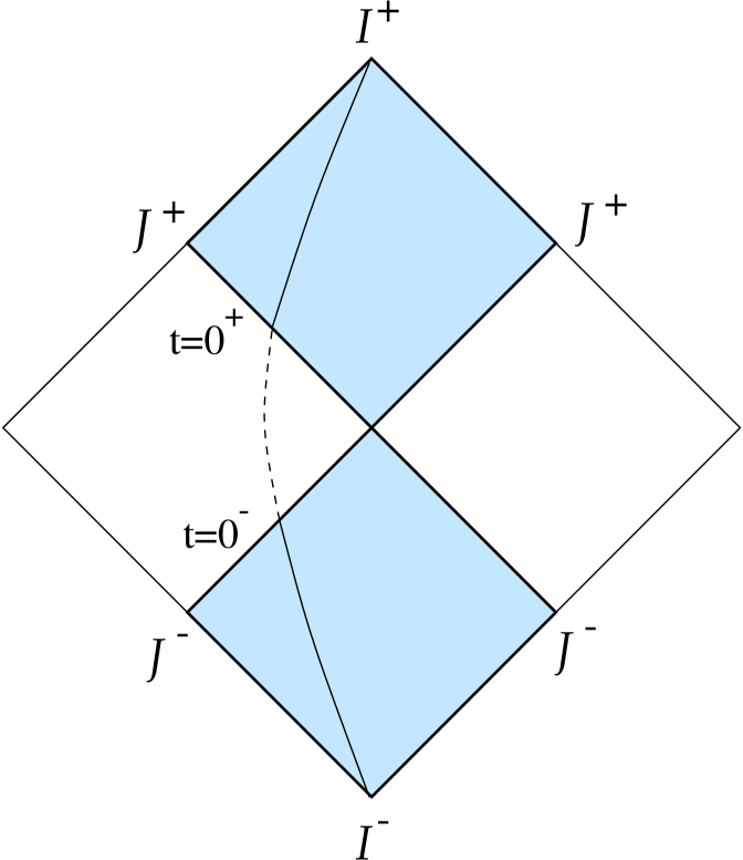
Figure 2: Our first method for constructing quantum fields on ${\cal M}$, illustrated in a conformal diagram of Minkowski space. The unitary map from the past light cone of the origin, $t=0^{-}$, to the future light cone $t=0^{+}$ is defined by free field evolution across the Rindler wedges to the left and right of the origin. Using this rule we obtain a unitary theory on the Milne universe ${\cal M}$, which may then be compactified into the space ${\cal M}_{C}$ shown in Figure 1.

IV Quantum Field Theory on ${\cal M}_{C}$

We shall describe several different constructions for quantum fields on ${\cal M}_{C}$, which all yield an essentially unique result.

The first method is based on Figure 2. We use the embedding of ${\cal M}_{C}$ in Minkowski spacetime to define the map from $t=0^{-}$ to $t=0^{+}$. This is possible as long as one or more of the $\vec{x}$ directions are noncompact, because in this case, the corresponding momenta $\vec{k}$ are continuous and $\vec{k}=0$ is a set of measure zero. From the two dimensional standpoint, this means that all modes are effectively massive. And for massive fields, free field evolution provides a unitary map between the past light cone of the origin ($t=0^{-}$) and the future light cone ($t=0^{+}$), because no information can be carried off to null infinity $J^{+}$. The coordinate $t$ analytically continues to a spacelike coordinate in the Rindler wedges, and as one follows the trajectory plotted in Figure 2, this coordinate runs from zero to a finite value then back to zero. So in effect a ‘clock’ measuring $t$ makes no progress whilst the trajectory is outside the region ${\cal M}$ of interest.

Figure 3: Integration contours used to define the positive and negative frequency modes on the entire Milne universe ${\cal M}$.

This first method may also be viewed as a certain analytic continuation in the complex $t$-plane (Figure 3). The field equation is analytic in the original Minkowski coordinates $T$ and $Y$ so the global solution may be obtained unambigously by analytic continuation in those coordinates. We shall show that this corresponds to the continuation of the positive and negative frequency mode functions $\Psi^{(+)}$ and $\Psi^{(-)}$ from negative to positive $t$, illustrated in the diagram above. The positive frequency mode functions so defined are analytic in the lower half $t$-plane, and the negative frequency mode functions are analytic in the upper half $t$-plane. The quantum field, being a sum of the positive and negative frequency modes, is continued in this mixed fashion across $t=0$. This analytic continuation method is actually more fundamental than continuation across the Rindler wedges, because it does not involve those unphysical regions. This is an important distinction when we introduce interactions. There is an ambiguity (for example about what the mass used in the free field propagation should be) in the Minkowski space continuation, but no corresponding ambiguity in the method illustrated in Figure 3.

Nevertheless it is interesting to discuss in more detail how the two methods correspond, for free fields. The coordinate $t$ continues to a spacelike variable $t=\pm is$ in the Rindler regions, where the line element is $ds^{2}-s^{2}dy^{2}$, and $y$ is now timelike. So in the Rindler regions, the continuation across from $t=0^{-}$ to $t=0^{+}$ occurs via paths which run up (or down) the imaginary $t$ axis and back again. On these paths, $y$ is also evolving from $-\infty$ to $+\infty$. Modes with nonzero momentum $k_{y}$ in the Milne region undergo an infinite number of oscillations as they approach $t=0^{-}$ from above or below, and an infinite number more as they cross the Rindler wedges. More subtle is the behaviour of the $k_{y}=0$ modes. As we discussed, these modes generically diverge logarithmically as one approaches $t=0^{-}$. By a choice of phase one can put this divergence into the imaginary part of the mode functions. Then, as one circumnavigates the origin in the complex $t$-plane, the logarithm aquires an imaginary part of $\pm i\pi$. This causes the real part of the mode functions to undergo a jump, of just the amount needed to reverse its sign. This is illustrated in Figure 4.

Figure 4: Behaviour of the $k_{y}=0$ modes as they cross $t=0$. With our choice of phase, the imaginary part (Im) diverges logarithmically but the real part (Re) is finite. Analytic continuation along the path shown in Figure 3 causes the real part to be odd in $t$ whereas the imaginary part is even.

The method described above is, we believe, completely adequate for dealing with quantum fields on ${\cal M}_{C}$. However, it is also interesting an important to develop the corresponding description of passage through the singularity in the $d$ dimensional effective theory. In this theory, a scalar field has action

$$-\int dtd^{d-1}\vec{x}|t|{1\over 2}\eta^{\mu\nu}\partial_{\mu}\varphi\partial_{\nu}\varphi,$$ (6)

with a specific time dependence in the kinetic term. Our approach here will be to regularize the theory by changing $|t|$ to $|t|^{1-\epsilon}$, with $\epsilon$ a parameter analogous to that in dimensional regularization, to be taken to zero after renormalization. It is then necessary to add counterterms to the Hamiltonian at $t=0$ in order to render the time evolution operator well defined in the $\epsilon\rightarrow 0$ limit. These counterterms have the effect of inducing a shift in the scalar field, proportional to its momentum, and analogous to the jump produced in the analytic continuation method illustrated in Figure 4. This shift cancels divergences and renders the final state well defined. We shall show that within this method, demanding that the counterterms be local in $\vec{x}$, and imposing time reversal symmetry is enough to uniquely fix the vacuum state.

Finally, we shall point out an intriguing mapping between this problem and that of free fields on de Sitter spacetime. Under this mapping, the surface $t=0^{+}$ corresponds to the past timelike infinity in de Sitter space, and $t=0^{-}$ corresponds to future timelike infinity. While these two surfaces are only connected at a point in the Milne universe, they are connected by a smooth bulk (comprising the entire spacetime) in the de Sitter case. The matching in de Sitter spacetime is unambiguous and again we shall show it corresponds to the previously obtained results. There are holographic elements of this correspondence. Holography is naturally framed in terms of null surfaces[13], and our approach involves matching information located on the two null surfaces $t=0^{-}$ and $t=0^{+}$. However, when we map to de Sitter spacetime, these two surfaces map to two spacelike surfaces, future and past timelike infinity, which are those which have been employed in the proposed de Sitter-CFT correspondence [14].

All of these methods yield the same result for the quantum vacuum state on ${\cal M}_{C}$. Because there is no mixing of the positive and negative frequency modes, there is no particle production in the free field theory. However, once interactions are included, particle production occurs, and in Section VI we demonstrate that it is well defined. The $k_{y}\neq 0$ modes are produced with a density which tends to zero exponentially as $H_{5}$ vanishes, suggesting an adiabatic limit in which the particle production vanishes in the limit of slowly colliding boundary branes. The $k_{y}=0$ modes do not show this behaviour, but we shall discuss how within string theory we can anticipate how an adiabatic limit may in fact emerge.

Finally, let us mention the connection between this work and other, more ambitious attempts to directly construct string theory on the compactified Milne spacetime considered here. Nekrasov[16] considered string theory on the Lorentzian orbifold constructed by orbifolding Minkowski spacetime by a boost. In that construction, the two Rindler wedges become compactified in a timelike direction, producing two extra cones projecting horizontally from the origin, which possess closed timelike curves. Additionally, line segments emanating from the origin are produced in each of the four null directions. Cornalba and Costa avoid these features by modding out by a boost combined with a translation, replacing them instead by a new region containing a naked timelike singularity[17]. Balasubramanian et al. consider other examples of time-dependent orbifold backgrounds in string theory. Whilst free strings seem to be well defined in these backgrounds, it is not yet clear whether interactions can be consistently introduced.

The approach we suggest here does not amount to orbifolding Minkowski space. Instead, we use free field evolution (or, equivalently analytic continuation in $t$) to define a matching rule between the big crunch and the big bang. This difference is unimportant in the free theory, since the only difference in that case between our approach and the orbifold approach is that we would declare that the extra regions in the orbifold approaches do not exist. It is when we introduce interactions that the difference becomes crucial. In our case, the interaction Lagrangian is only integrated over the physical compactified Milne spacetime, whereas in the orbifold approaches it would be integrated over the additional regions too, containing closed time-like curves or naked singularities. We should stress that we have not attempted to construct string theory in our approach, therefore we cannot say whether string theory will ultimately be consistent on compactified Milne. However the field theory results are suggestive and we hope they will be a guide to such a construction.

V Embedding Milne in Minkowski

V.1 Positive and Negative Frequency modes

In this section we describe our first construction of quantum field theory on ${\cal M}_{C}\times R^{d-1}$. A Fourier mode of a massless field, $\varphi(t,y,\vec{x})=\varphi(t)e^{i(\vec{k}\cdot\vec{x}+k_{y}y)}$, obeys the field equation

$$\ddot{\varphi}+{1\over t}\dot{\varphi}+{k_{y}^{2}\over H_{5}^{2}t^{2}}\varphi+m^{2}\varphi=0,$$ (7)

where dot denotes partial derivative with respect to $t$. We have introduced the effective two dimensional mass $m^{2}\equiv\vec{k}^{2}$, and henceforth the $\vec{x}$ dependence shall play a purely spectator role. Equation (7) is just Bessel’s equation, with imaginary order $\nu=ik_{y}/H_{5}$. It has a singular point at $t=0$. The solutions which tend to positive and negative frequency WKB modes at late times are the Hankel functions, and the properly normalised outgoing positive and negative frequency modes are

$$\psi^{+}_{k_{y}}=\sqrt{\frac{\pi}{4H_{5}}}e^{{\pi k_{y}\over 2H_{5}}}H^{(2)}_{ik_{y}/H_{5}}(mt)e^{ik_{y}y},\qquad\psi^{-}_{k_{y}}=\sqrt{\frac{\pi}{4H_{5}}}e^{-{\pi k_{y}\over 2H_{5}}}H^{(1)}_{ik_{y}/H_{5}}(mt)e^{ik_{y}y}.$$ (8)

We would like to continue these modes to negative times. The Hankel functions have the following integral representations

$$H^{(1)}_{\nu}(z)=\frac{e^{-{i\pi\nu\over 2}}}{\pi i}\int_{-\infty}^{\infty}du\exp({iz\cosh u-\nu u}),$$ (9)

which is analytic in the upper half $z$-plane, and

$$H^{(2)}_{\nu}(z)=-\frac{e^{{i\pi\nu\over 2}}}{\pi i}\int_{-\infty}^{\infty}du\exp({-iz\cosh u-\nu u}),$$ (10)

which is analytic in the lower half $z$-plane. Consequently the Milne mode functions can be expressed as

$$\psi^{+}_{k_{y}}=\frac{i}{2}\sqrt{\frac{1}{\pi H_{5}}}\int_{-\infty}^{\infty}du\exp({-imt\cosh u-i\frac{k_{y}}{H_{5}}(u-H_{5}y)}),\qquad\psi^{-}_{k_{y}}=\psi^{+*}_{k_{y}}.$$ (11)

By shifting the integration variable $u\rightarrow u+yH_{5}$, we obtain

$$\psi^{+}_{k_{y}}=\frac{i}{2}\sqrt{\frac{1}{\pi H_{5}}}\int_{-\infty}^{\infty}du\exp({-imt\cosh u\cosh H_{5}y-imt\sinh u\sinh H_{5}y-i\frac{k_{y}}{H_{5}}u}).$$ (12)

Further changing variables to $K_{Y}=-m\sinh(u)$ gives

$$\psi^{+}_{k_{y}}=\frac{i}{2}\sqrt{\frac{1}{\pi H_{5}}}\int_{-\infty}^{\infty}\frac{dK_{Y}}{\sqrt{K_{Y}^{2}+m^{2}}}e^{i{k_{y}\over H_{5}}\sinh^{-1}(K_{Y}/m)}\exp(iK_{Y}Y-i\sqrt{K_{Y}^{2}+m^{2}}T),$$ (13)

where $T=t\cosh(H_{5}y)$ and $Y=t\sinh(H_{5}y)$ are the embedding co-ordinates in Minkowski space. This is a superposition of positive frequency plane wave modes on Minkowski space with momentum $K_{Y}$. We note that the right hand side is an oscillatory integral which can be defined for $t<0$ by inserting a suitable convergence factor. Therefore the integral representation may be used as the definition of the mode functions there.

The above integral representations of the Hankel functions define a natural analytic continuation across $t=0$. One can read off from (9) and (10) the relations

$$H^{(2)}_{\nu}(e^{-i\pi}z)=-e^{i\pi\nu}H^{(1)}_{\nu}(z),\qquad H^{(1)}_{\nu}(e^{i\pi}z)=-e^{-i\pi\nu}H^{(2)}_{\nu}(z).$$ (14)

To see what these imply for the $k_{y}=0$ modes, recall that

$$H^{(1)}_{0}(mt)\equiv J_{0}(t)+iN_{0}(t),\qquad H^{(2)}_{0}(mt)\equiv J_{0}(t)-iN_{0}(t).$$ (15)

The rule (14) implies that the analytic continuation of $H^{(2)}_{0}(mt)$ to negative values is $-J_{0}(-t)-iN_{0}(-t)$. Therefore from (15) the real part of $H^{(2)}_{0}(mt)$ is an odd function of $t$, with a discontinuity at $t=0$, and the imaginary part is even, with a logarithmic divergence at $t=0$. The real and imaginary parts are illustrated in Figure 4.

From the integral representations (9) and (10) one can determine the behaviour of the analytically continued Hankel functions at large positive or negative $t$ by performing the integral via the stationary phase method, obtaining

$$H^{(2)}_{ik_{y}/H_{5}}(mt)\sim-{e^{-\pi k_{y}\over 2}\over i\pi}e^{-imt}\sqrt{2\pi\over|mt|}e^{\mp i\pi\over 4}\quad t\rightarrow\pm\infty,$$ (16)

and similarly for $H^{(1)}_{ik_{y}/H_{5}}(mt)$, with $i\rightarrow-i$ and $k_{y}\rightarrow-k_{y}$. This continuation implies that there is no particle production since positive frequency incoming modes are matched to only positive frequency outgoing modes.

It is important to stress that this choice of vacuum is priviledged. As we explained earlier if we cut off the singularity in a crude way, then for a generic choice of $|in>$ and $|out>$ states, for each $\vec{k}$ we would obtain in the $k_{y}=0$ mode a particle production rate that diverges logarithmically with the regulator. It is only for the special case in which we define $|out>=|in>$ or at least some finite Bogoliubov transformation of the $|in>$ state that we obtain a finite result. From the $d$ dimensional perspective this seems contrived, but from the $d+1$ dimensional picture and the embedding in Minkowski space it is clearly the most natural choice. In later sections we shall also justify this matching from a purely $d$ dimensional point of view.

Finally, let us mention that our definition of in and out vacuum modes is not the same as that which has conventionally been used in treatments of quantum fields on Milne spacetime (see for example, Ref. References). In previous work, only the $t>0$ part of ${\cal M}$ was used, and the initial vacuum was taken to be the ‘conformal vacuum’ as $t\rightarrow 0^{+}$, defined by the ‘positive frequency’ modes behaving as $e^{-ik_{y}\tau}$ as the conformal time $\tau\rightarrow-\infty$. This is of course, not an adiabatic vacuum state, and therefore a somewhat arbitrary choice. In the conformal vacuum state, one finds particle production occurs in passing from the big bang $t\rightarrow 0^{+}$ to the asymptotic future, even in free field theory[18].

V.2 Projection onto ${\cal M}_{C}$

We have not yet distinguished between the Milne space ${\cal M}$ and its compactification ${\cal M}_{C}$, which as we described above equation (3) is just ${\cal M}/\Gamma(H_{5}L)$, with $\Gamma(H_{5}L)$ the group of boosts with rapidity $H_{5}L$.

In Minkowski spacetime a particle is defined in a group theoretic sense as an irreducible projective representation of the Poincare group. We can similarly define particles on ${\cal M}_{C}$ by using representations on the covering Minkowski space that are invariant under the action of the boost $\Gamma(H_{5}L)$. The map from Milne to Minkowski introduced in the previous section is inverted by means of a Fourier transform, to obtain

$$\Psi_{K_{Y}}(Y,T)=e^{iK_{Y}Y-i\sqrt{K_{Y}^{2}+m^{2}}T}=\int_{-\infty}^{\infty}\frac{dk_{y}}{2\pi}e^{\pi k_{y}\over 2H_{5}}H^{(2)}_{ik_{y}/H_{5}}(mt)e^{ik_{y}(y-H_{5}^{-1}\sinh^{-1}(\frac{K_{Y}}{m}))}$$ (17)

The plane waves $\Psi_{K_{Y}}(Y,T)$ form a representation of the two dimensional Poincare group, and the action of the boost $\Lambda$ on these modes can be expressed as

$$\Lambda:\Psi_{K_{Y}}(Y,T)\rightarrow\Psi_{K_{Y}}(\Lambda Y,\Lambda T)$$ (18)

where $(\Lambda Y,\Lambda T)=(t\sinh(H_{5}(y+L)),t\cosh(H_{5}(y+L)))$ is simply a translation by $L$ in $y$. A representation of the group $Poincare/\Gamma(H_{5}L)$ can be constructed by simply summing over all boosts,

$$\tilde{\Psi}_{K_{Y}}(Y,T)=\sum_{n=-\infty}^{\infty}\Psi_{K_{Y}}(\Lambda^{n}(H_{5}L)Y,\Lambda^{n}(H_{5}L)T)=\sum_{n=-\infty}^{\infty}\Psi_{K_{Y}}(\Lambda(nH_{5}L)Y,\Lambda(nH_{5}L)T).$$ (19)

We shall only use these functions on the physical region of interest, namely ${\cal M}_{C}$, where they are given by

$$\tilde{\Psi}_{K_{Y}}(Y,T)=\sum_{n=-\infty}^{\infty}\int_{-\infty}^{\infty}\frac{dk_{y}}{2\pi}e^{\pi k_{y}\over 2H_{5}}H^{(2)}_{ik_{y}/H_{5}}(mt)e^{ik_{y}(y+nL-H_{5}^{-1}\sinh^{-1}(\frac{K_{Y}}{m}))}.$$ (20)

Now using the Poisson summation formula $\sum_{n=-\infty}^{\infty}\int_{-\infty}^{\infty}dte^{2\pi int}f(t)=\sum_{m=-\infty}^{\infty}f(m)$, we obtain

$$\tilde{\Psi}_{K_{Y}}(Y,T)=\frac{1}{L}\sum_{n=-\infty}^{\infty}e^{\pi^{2}n\over H_{5}L}H^{(2)}_{2i\pi n/H_{5}L}(mt)e^{i{2\pi n\over L}(y-H_{5}^{-1}\sinh^{-1}(\frac{K_{Y}}{m}))}.$$ (21)

This is just the expected result that summing over boosts projects out only those states that are translation invariant under $y\rightarrow y+L$, and is equivalent to quantizing the momentum $k_{y}=2\pi n/L$. If we were to perform the further projection onto the orbifold $S_{1}/Z_{2}$ mentioned in the introduction, we would now consider separating the $k_{y}$ modes into those which are odd and even under $y\rightarrow L-y$. In string theory, this step introduces new states (‘twisted states’) but for field theory describing quantum mechanical particles, it has no such effect.

The Feynman propagator on ${\cal M}$ is obtained by simply restricting the $d+1$ dimensional Minkowski space propagator to the Milne region. In $d+1$ dimensions the Feynman propagator is [19]

$$G_{F}(x,x^{\prime})=-i{\pi\over(4\pi i)^{d+1\over 2}}\left({m^{2}\over\sigma+i\epsilon}\right)^{d-1\over 4}H_{(d-1)/2}^{(2)}(m(-\sigma-i\epsilon)^{1/2}),$$ (22)

where $x=(T,Y,\vec{x})$ and $\sigma=(\vec{x}-\vec{x}^{\prime 2})+(Y-Y^{\prime})^{2}-(T-T^{\prime})^{2}$. Restricting the Feynman propagator to the Milne patch simply requires writing $\sigma$ in terms of the Milne co-ordinates $\sigma(x,x^{\prime})=(\vec{x}-\vec{x}^{\prime})^{2}-(t-t^{\prime})^{2}-4tt^{\prime}\sinh^{2}(H_{5}(y-y^{\prime})/2)$. The Feynman propagator on the compactified Milne spacetime is obtained by projecting onto the boost invariant states. This is given by

$$G^{{\cal M}_{C}}_{F}(x,x^{\prime}) = \sum_{n=-\infty}^{\infty}G^{\cal M}_{F}(\Lambda^{n}(H_{5}L)x,x^{\prime})$$ (23)

$$= \sum_{n=-\infty}^{\infty}-i{\pi\over(4\pi i)^{d+1\over 2}}\left({m^{2}\over\sigma_{n}+i\epsilon}\right)^{d-1\over 4}H_{(d-1)/2}^{(2)}(m(-\sigma_{n}-i\epsilon)^{1/2})$$ (24)

where $\sigma_{n}(x,x^{\prime})=(\vec{x}-\vec{x}^{\prime})^{2}-(t-t^{\prime})^{2}-4tt^{\prime}\sinh^{2}(H_{5}(y+nL-y^{\prime})/2)$. The Feynman propagator, in addition to the interaction vertices, is all one needs in order compute the $S$ matrix via perturbation theory on ${\cal M}_{C}$.

V.3 UV divergence behaviour

It is important to understand whether compactifying Minkowski spacetime into ${\cal M}_{C}\times R^{d-1}$ introduces any new ultraviolet divergences. For the construction given above, the free field propagator on ${\cal M}$ is just the Minkowski space propagator evaluated on ${\cal M}$. Therefore it has just the usual divergences. In this section we shall show that the same is true for the propagator on ${\cal M}_{C}$, for all points $x$ and $x^{\prime}$ away from $t=0$. This is to be expected intuitively since the Green functions on ${\cal M}_{C}$ are constructed by summing over boosts on one argument $x$, and these boosts carry $x$ further and further from $x^{\prime}$.

The difference between the Feynman propagator on $\cal{M}_{C}$ and $\cal{M}$ is given in $d+1$ dimensions by

$$\Delta G_{F}(x,x^{\prime})=\sum_{n=-\infty,\neq 0}^{\infty}-i{\pi\over(4\pi i)^{d+1\over 2}}\left({m^{2}\over\sigma_{n}+i\epsilon}\right)^{d-1\over 4}H_{(d-1)/2}^{(2)}(m(-\sigma_{n}-i\epsilon)^{1/2}),$$ (25)

which in the coincidence limit $x^{\prime}=x$ becomes

$$2\sum_{n=1}^{\infty}-i{\pi\over(4\pi i)^{d+1\over 2}}\left({m^{2}\over-4t^{2}\sinh^{2}(H_{5}nL/2)+i\epsilon}\right)^{d-1\over 4}H_{(d-1)/2}^{(2)}(m(4t^{2}\sinh^{2}(H_{5}nL/2)-i\epsilon)^{1/2}).$$ (26)

The large $|z|$ asymptotic behaviour of the Hankel function is $H_{\nu}^{(2)}(z)\rightarrow(\frac{2}{\pi z})^{1/2}e^{-i(z-\frac{1}{2}\nu\pi-\frac{1}{4}\pi)}$ and so the sum is rapidly convergent for nonzero $t$. Thus, at least away from $t=0$ the UV divergence behaviour of the Green function on ${\cal M}_{C}$ is just the same as that on Minkowski space. The behaviour of the Green function at $t=0$ is a more delicate matter, linked to the way in which interactions enter, which we shall discuss below.

In the next section we shall see that if interactions are introduced on ${\cal M}$ as integrals over fields on ${\cal M}$, there are physical processes such as particle creation from the vacuum that occur at tree level, and which have no counterpart in Minkowski spacetime. They arise because energy is no longer conserved when the interactions are time-dependent.

VI Interacting Field Theory

The prescription discussed above for matching the big crunch phase to the big bang phase in the Milne universe relied on free field theory. That is, in the Minkowski spacetime within which the Milne universe is embedded, we are propagating the fields according to the free field equations from the past light cone (on which Milne time is $t=0^{-}$) to the future light cone (on which Milne time is $t=0^{+}$). With this prescription, as we have emphasized, there is no particle production. However, once interactions are included, particles are generically produced because the interaction terms in the Hamiltonian are time dependent. We shall calculate this effect in this section, using a very simple toy model of the interactions. This is not intended to accurately represent the actual interactions in string theory, but we hope will illustrate the general behaviour including the sensitivity to infrared and ultraviolet cutoffs. The former should come from cosmological evolution, since the growth of the extra dimension ceases when the universe becomes radiation dominated. Ultraviolet divergences have to be controlled by string theory or M theory effects and we shall comment on the possible form of these below. It is important to stress that we use the Minkowski embedding only to determine a matching condition in the free field theory. The interacting theory lives on the physical spacetime ${\cal M}_{C}$. This is the sense in which our approach differs from one employing an interacting theory on a Lorentzian orbifold which is Minkowski space modulo a boost.

As a very simple example, consider an interaction of the form ${\cal S}=-\int{1\over 2}\mu^{2}\varphi^{2}$, where the integral runs only over ${\cal M}_{C}$. For concreteness we shall take $d=4$, so there are three noncompact dimensions $\vec{x}$. The interaction is simply a mass term, which from the point of view of the embedding theory in Minkowski space, is turned off outside the future and past light cones. We would like to compute the particle production due to this interaction. The quantum field $\varphi$ is expanded in terms of creation and annihilation operators as

$$\varphi=\int{d^{3}\vec{k}\over(2\pi)^{3}}\sum_{k_{y}}\left[a_{{k_{y}},\vec{k}}\psi^{+}_{k_{y}}e^{i{k_{y}}y+i\vec{k}.\vec{x}}+{\rm h.c.}\right],$$ (27)

where the $\vec{k}$ dependence of the modes is not explicitly shown. The creation and annihilation operators are normalized to obey

$$\left[a_{{k_{y}},\vec{k}},a_{{k^{\prime}_{y}},\vec{k^{\prime}}}^{\dagger}\right]=\delta_{{k_{y}},{k_{y}^{\prime}}}(2\pi)^{3}{\delta}^{3}(\vec{k}-\vec{k^{\prime}}).$$ (28)

We may now compute the transition amplitude between the incoming vacuum state and an outgoing state with two particles, with equal and opposite momenta $k_{y}$ and $\vec{k}$. The calculation is straightforwardly performed by first integrating over $y$ to obtain the delta function $\delta_{k_{y}+k_{y}^{\prime},0}$ corresponding to momentum conservation. Then we use the representation of the Hankel functions given in (13), evaluated at $Y=0$, $T=t$, to obtain the interaction matrix element

$${-i\mu^{2}\over 8H_{5}\pi V}(2\pi)^{3}\delta^{3}(\vec{k}+\vec{k}^{\prime})\int dt|t|\int\int dudu^{\prime}e^{i(u-u^{\prime}){k_{y}\over H_{5}}}e^{-i({\rm cosh}u+{\rm cosh}u^{\prime})mt}e^{-\epsilon|t|},$$ (29)

where we have inserted a Lorentz invariant convergence factor, and include the volume factor needed to normalise the final states (since $(2\pi)^{3}{\delta}^{3}(0)=V)$. The integrals are straightforwardly performed using the identity

$$\int_{-\infty}^{\infty}dx{{\rm cos}{k_{y}x}\over{\rm cosh}^{2}(x/2)}={4k_{y}\pi\over{\rm sinh}(k_{y}\pi/H_{5})},$$ (30)

to give

$$\langle{k_{y}},\vec{k},{k^{\prime}_{y}},\vec{k^{\prime}},{\rm out}|0,{\rm in}\rangle={i\mu^{2}\over 2m^{2}H_{5}V}(2\pi)^{3}\delta^{3}(\vec{k}+\vec{k}^{\prime})\delta_{k_{y}+k_{y}^{\prime},0}\,{(k_{y}/H_{5})\over m^{2}{\rm sinh}(k_{y}\pi/H_{5})}.$$ (31)

The probability for a transition from the vacuum to two particles with momenta $k_{y}=\pm 2\pi n/L$ and $\vec{k}$ within $d^{3}\vec{k}$ is therefore

$${\mu^{4}\over 16}V{d^{3}\vec{k}\over(2\pi)^{2}}{1\over|\vec{k}|^{4}}{(k_{y}/H_{5})^{2}\over{\rm sinh}^{2}(k_{y}\pi/H_{5})}.$$ (32)

Dividing by the volume $V$ one obtains the probability per unit volume for creating such particle pairs. At fixed external momentum, the final density of pairs is finite, as claimed. Furthermore, the $k_{y}\neq 0$ modes which naively might be thought to be the most dangerous, are strongly suppressed. As the rate $H_{5}$ of contraction of the extra dimension is decreased, the production of these Kaluza Klein modes becomes exponentially small, showing the existence of an adiabatic limit. The $k_{y}=0$ modes do not however display such a limit, and in fact the result for particle creation for these modes is completely independent of $H_{5}$. We shall discuss how this behaviour is likely to be altered in string theory, below.

The integration over $\vec{k}$ in (32) is infrared divergent. This is however an artefact of the fact that the interaction term we introduced diverges as $t\rightarrow\pm\infty$. In the situations of interest for the cyclic and ekpyrotic models, the extra dimension tends to a maximum size $t<<0$ and $t>>0$ and this would introduce an infrared cutoff in $|\vec{k}|$ of order $T_{C}^{-1}$ where $T_{C}$ is the characteristic time scale over which Milne-like behaviour holds. The total number density of created particles with this simple $\varphi^{2}$ interaction is ultraviolet finite. But the total energy density is logarithmically divergent. This disease may be cured by introducing the dilaton $\phi$ into the nonlinear field interactions, which generically occurs in string theory. We have $e^{\phi\sqrt{(d-2)/(d-1)}}\propto|t|$, and each extra power of $|t|$ in the interaction introduces an extra negative power of $|\vec{k}|$ in the matrix element, or $|\vec{k}|^{-2}$ in the probability. Conversely, if we introduce higher powers of $\varphi$ in the interaction, e.g. $\varphi^{3}$, this would boost the rate in the ultraviolet, just because more particles are created in each process and the phase space integral would involve a higher overall power of $\vec{k}$. (Recall, there is no conservation of energy here since we have explicitly broken time translation invariance). Again, we can make the produced number or energy density finite by introducing sufficient powers of the dilaton coupling. However, as we shall now explain, we believe there should be additional effects suppressing the rate of production of particles with high momentum in string theory.

The origin of the power law fall-off in these calculations may be traced to the sharpness in time $t$ of the simple field theory interaction term we have introduced, and the fact that this interaction cannot be correct for very high momenta of the external particles. The Fourier transform of a function with a sharp kink falls off only as a power law, so with this field theory interaction, high energy energy-nonconserving processes are only suppressed as a power law of the energy. If interactions can be consistently introduced in string or M theory on ${\cal M}_{C}$, we believe they will not show this sharp behaviour. Strings or membranes are never localised below a minimal length scale $l_{s}$, and one would expect them not to see the extra dimension shrink below a minimal length scale $l_{s}$. One could model this by replacing the factor $H_{5}|t|L$, which is the length of the extra dimension, with $\sqrt{l_{s}^{2}+H_{5}^{2}L^{2}t^{2}}$, which never falls below $l_{s}$. If we make this replacement in the particle production just computed, then the final particle density is actually exponentially convergent in the ultraviolet. Returning to (29), we see it is dominated by $u\sim u^{\prime}\sim 0$. The effect of introducing the cutoff $l_{s}$ is therefore roughly the replacement

$$\int dt|t|e^{-imt-\epsilon|t|}\rightarrow\int dt\sqrt{t^{2}+\delta^{2}}e^{-imt-\epsilon|t|},$$ (33)

where $\delta=l_{s}/(H_{5}L)$. The left hand side equals $-2/m^{2}$ as $\epsilon\rightarrow 0$. This exhibits the power law dependence of our answer for the amplitude above. However, for large $m\delta$ the right hand side decays exponentially in $m\delta$. To see this, compute the difference between the left and right hand sides of (33), in which $\epsilon$ may be set to zero from the outset. By integrating by parts, one can reduce the difference to

$$-{2\over m^{2}}+\int_{0}^{\infty}{dt\over m^{2}}{\rm cos}(mt){\delta^{2}\over(t^{2}+\delta^{2})^{3\over 2}}.$$ (34)

It follows that the integral equals minus the right hand side of (33). The latter is a Hankel function of imaginary argument, which decays exponentially, as $e^{-m\delta}=e^{-ml_{s}/(H_{5}L)}$, for large $ml_{s}$ (i.e. particle momenta well above the string scale), or for small $H_{5}L$ (i.e. a small contraction speed of the extra dimension).

Two important things occur in this model. First, the cutoff is not at the string scale, it is at $|\vec{k}|\equiv m\sim(H_{5}L)/l_{s}$. More importantly, for fixed $|\vec{k}|$, the particle production becomes exponentially small as $H_{5}L$ is lowered below $|\vec{k}|l_{s}$. This means that for $H_{5}L<<1$ and for modes of any fixed physical wavelength in the non-compact direction, there is an adiabatic limit in which the extra dimension can disappear and reappear with vanishingly small particle production. It remains to be seen whether these two desirable features will survive in a complete string theoretic calculation.

VII The d Dimensional Perspective

The cyclic and ekpyrotic universe scenarios represent attempts at consistent cosmologies based on M and string theory. The resolution of what happens at big bang/big crunch singularities must be found within those theories. If, for example, the extra dimension involved is the eleventh dimension of M theory, as represented in the model of Horava-Witten, then when the two boundary branes approach the theory reduces to weakly coupled heterotic string theory. The full dynamics of the eleven dimensional theory involves eleven dimensional supergravity and the associated super-membrane. Nevertheless, one hopes that at least for slow motions, the system evolves quasi-adiabatically and at small brane separations one is in the regime of ten dimensional string theory. Furthermore, since the string coupling constant vanishes as the extra dimension disappears, string interactions should be suppressed at the singularity itself. However, as noted in Ref. References, the description of the bounce in string theory may not be straightforward, because the ten dimensional string frame metric vanishes at the boundary brane collision.

In this section we shall attempt to describe not string theory but quantum field theory from a purely $d$ dimensional perspective. As in the string theory case, the $d$ dimensional metric will vanish at the singularity. Nevertheless we shall see that the singularity may be traversed in a reasonably natural manner.

The $d$ dimensional Einstein frame geometry corresponding to the $d+1$ Milne geometry considered earlier is given by

$$ds^{2}=|H_{5}t|^{2/(d-2)}(-dt^{2}+{d\vec{x}}^{2})$$ (35)

Note that the proper time $t$ of the $d+1$ geometry is identical to the conformal time $t$ of the $d$ dimensional Einstein frame geometry. The equation of motion of a massless scalar field is

$$t^{2}\ddot{\varphi}+t\dot{\varphi}+t^{2}\vec{k}^{2}\varphi=0,$$ (36)

just the equation for the $k_{y}=0$ mode of a $d+1$ dimensional massless scalar. Using the higher dimensional point of view as our guide we are lead to believe that the natural ‘in’ and ‘out’ states are

$$\psi^{out,+}(t,x)=\psi^{in,+}(t,x)=\sqrt{\frac{\pi}{4H_{5}}}H^{(2)}_{0}(|\vec{k}t|)e^{i\vec{k}\cdot\vec{x}},$$ (37)

and the corresponding Wightman function is

$$G^{+}(x,x^{\prime})=\int\frac{d^{d}\vec{k}}{(2\pi)^{d}}\frac{\pi}{4H_{5}}H_{0}^{(2)}(|\vec{k}|(t-i\epsilon))H_{0}^{(1)}(|\vec{k}|(t+i\epsilon))e^{i\vec{k}\cdot(\vec{x}-\vec{x}^{\prime})}$$ (38)

How can we understand why this is natural purely from a $d$ dimensional point of view? As already discussed in Section III, regulating the spacetime in the sense of $|t|\rightarrow\sqrt{t^{2}+\delta^{2}}$ will generically produce a particle production that diverges as $\ln(H_{5}\delta)$. The fact that this divergence is identical for each $\vec{k}$ suggests that it may be removed by a counterterm which is local in $d$ dimensions.

VII.1 What renormalization?

How should we remove the logarithmic divergence in the scalar field as it approaches the singularity? From the $d$ dimensional perspective, we would like to follow the traditional renormalization program: regularizing the theory, adding counterterms and finally removing the regulator. But we need to discuss what form the renormalization should take.

As mentioned above, in the limit when $t$ tends to zero, the dynamics of the field are dominated by the kinetic term. This term possesses a symmetry $t\rightarrow\lambda t$ (which is just a translation in conformal time). The scalar field tends to $\varphi\sim A+B{\rm ln}|H_{5}t|$, and its momentum $\pi$ tends to $H_{5}B$. Rescaling time as above has the effect of increasing $\varphi$ by $B{\rm ln}\lambda$, or $H_{5}^{-1}\pi{\rm ln}\lambda$. Therefore it is very natural to seek to exploit such a shift in order to remove the divergence in $\varphi$. Since $\pi$ is asymptotically a constant, one can simply match it across $t=0$. But to make $\varphi$ finite, we need to redefine it via $\varphi\rightarrow\varphi+C\pi$, across the $t=0$ surface in the regulated theory, with the constant $C$ chosen to obtain finite correlators for $\varphi$ and $\pi$ for $t>0$, as the regulator is removed.

The shift $\varphi\rightarrow\varphi+C\pi$, $\pi\rightarrow\pi$, is a canonical transformation. It can be implemented by adding a a local counterterm to the Hamiltonian, which acts at $t=0$ to produce an additional unitary transformation taking the incoming to the outgoing quantum state. We shall show below that demanding the vacuum be both Hadamard and time reversal invariant uniquely fixes the value of the constant $C$.

VII.2 Dimensional Regularization

Before we can renormalize the $d$-dimensional theory we must first regularize it. We shall use a regularization which makes both the field and its canonical momentum finite at $t=0$, but which allows the background to remain a solution of the field equations everywhere except at $t=0$.

The dimensional regularization we use relies upon the generalization of the $1+1$ dimensional Milne universe we have so far studied to a $1+n$ dimensional Milne universe. Like their $1+1$ dimensional cousin these are just a re-writing of Minkowski spacetime, but in dimensions $n>1$ their constant time slices are negatively curved hyperboloids $H_{n}$. We therefore consider the following vacuum Einstein’s equations in $d+1$ dimensions,

$$ds^{2}=-dt^{2}+H_{5}^{2}t^{2}dH_{n}^{2}+\sum_{i=1}^{d-n}dx_{i}^{2},$$ (39)

where $dH_{n}^{2}$ is the line element on $H_{n}$. This is a solution of the $d+1$ dimensional field equations if the curvature (Ricci) scalar of the $H_{n}$ is $-n(n-1)H_{5}^{2}/2$. From the $d-n$-dimensional point of view, we are considering fields which are constant on the $H_{n}$, we have Einstein gravity plus a scalar field $\phi$ representing the ‘scale factor’ of the $H_{n}$. The spatial curvature term in the $d+1$ dimensional Einstein action leads to a potential for $\phi$ in the dimensionally reduced $d-n$ dimensional action, proportional to $n(n-1)$, and positive for $n>1$. The idea of the regularization we use is to analytically continue this reduced theory in $n$, and ultimately take the limit as $n\rightarrow 1$.

The action for a scalar field which is homogeneous on the $H_{n}$ is just

$$-{1\over 2}\int dt|H_{5}t|^{n}\eta^{\mu\nu}\partial_{\mu}\varphi\partial_{\nu}\varphi.$$ (40)

For $n=1-\epsilon$, with $\epsilon$ small and positive, it turns out that the field $\varphi$ and its canonical momentum $\pi$ are both finite at $t=0$ and therefore both can be simultaneously matched across $t=0$. To see this, note that as $t\rightarrow 0$ the scalar field equation is approximated by

$$t^{2}\ddot{\varphi}+(1-\epsilon)t\dot{\varphi}\approx 0,$$ (41)

with general solution $\varphi\sim A+B(H_{5}t)^{\epsilon}$. The momentum conjugate to $\varphi$ is given by $\pi=|H_{5}t|^{1-\epsilon}\dot{\varphi}\sim\epsilon H_{5}B$, constant in this limit. The remarkable feature is that for positive $\epsilon$, $\varphi$ is also finite at $t=0$, enabling us to match across $t=0$. (The limiting case $\epsilon=0$, which we studied before, can be obtained by expanding $(H_{5}t)^{\epsilon}\approx 1+\epsilon\ln(H_{5}t)$ for small $\epsilon$, and redefining the constants.)

Whilst it is important that we have constructed the regularized backgrounds as solutions of the field equations everywhere except at $t=0$, for the purposes of this section all that really matters is that we have regularized the action for the scalar $\varphi$ to (40) for $t<0$ and for $t>0$ so that we can match $\varphi$ and $\pi$ across $t=0$, with the introduction of local counterterms at that point.

VII.3 Matching Modes across the Singularity

The regularized field equation for the $y$-independent modes is

$$t^{2}\ddot{\varphi}+(1-\epsilon)t\dot{\varphi}+m^{2}t^{2}\varphi=0,$$ (42)

with $m^{2}\equiv\vec{k}^{2}$ as before. The general solution is $\varphi=(mt)^{(\epsilon/2)}\chi(mt)$, with $\chi$ a Bessel function of order $\epsilon/2$.

As $t$ tends to zero, solutions to the regularized equation tend to the form $\varphi\sim A+B|\vec{k}t|^{\epsilon}$, with $A$ and $B$ constants. Thus as claimed above, both $\varphi$ and $\pi\equiv|H_{5}t|^{1-\epsilon}\dot{\varphi}$ tend to constants as $t$ tends to zero. Let $(A^{-},B^{-})$ and $(A^{+},B^{+})$ denote the values of these constants for $t<0$ and $t>0$. Matching $\varphi$ and $\pi$ at $t=0$ gives $A^{+}=A^{-}$ and $B^{+}=-B^{-}$. Thus the asymptotic solutions for small $|\vec{k}t|$ are

$$\varphi\sim A+B{\rm sign}(t)|\vec{k}t|^{\epsilon}.$$ (43)

Using the asymptotic form of the Hankel functions for small argument and redefining the constants we find that the general solution for all $t$ is

$$\varphi=$$ (44)

$$|\vec{k}t|^{\epsilon/2}[C\left(e^{i\epsilon\pi/2}H^{(1)}_{\epsilon/2}(|\vec{k}t|)+e^{-i\epsilon\pi/2}H^{(2)}_{\epsilon/2}(|\vec{k}t|)\right)+D{\rm sign}(t)\left(H^{(1)}_{\epsilon/2}(|\vec{k}t|)+H^{(2)}_{\epsilon/2}(|\vec{k}t|)\right)].$$ (45)

As before defining the in and out states to be $\varphi_{in}=A_{\epsilon/2}H^{(1)}_{\epsilon/2}(-|\vec{k}|t)$ for $t<0$ and $\varphi_{out}=A_{\epsilon/2}H^{(2)}_{\epsilon/2}(|\vec{k}|t)$ for $t>0$ we find the following relation between the in and out states:

$$\varphi_{in}=\alpha\varphi_{out}+\beta\varphi^{*}_{out},\qquad\alpha=-i{\rm cosec}(\pi\epsilon/2)e^{-i\pi\epsilon/2},\qquad\beta=-i\cot(\pi\epsilon/2).$$ (46)

Let us consider the limit $\epsilon\rightarrow 0$. In this limit $\alpha\rightarrow-2i/(\pi\epsilon)$ and $\beta\rightarrow-2i/(\pi\epsilon)$. This implies infinite particle production, as we obtained before with the simple cutoff. In fact the analogy is

$$\frac{1}{\epsilon}\approx\ln(\frac{1}{H_{5}\delta}).$$ (47)

This relationship is similar to that obtained in ordinary renormalization where $1/(d-4)$ divergences in dimensional regularization corresponds to the $\ln(\Lambda)$ divergences obtained with a UV cutoff.

VII.4 Regularization Independence

In the previous section we have seen that the logarithmic divergences of the naive cutoff regularization used earlier manifest themselves as $1/\epsilon$ divergences in the dimensional regularization scheme. We now want to renormalize these divergences, by absorbing the divergent pieces in local counterterms added to the action.

In dimensional regularization the minimal subtraction scheme is simply to throw away $1/\epsilon$ divergences. Here, one must be more careful since there is a danger of violating unitarity. We are able to perform the subtraction via a unitary transformation as follows. First write the Bogoliubov transformation in the form

$$\left(\begin{array}[]{cc}\varphi_{out}\\ \varphi_{out}^{*}\\ \end{array}\right)=\left(\begin{array}[]{cc}\alpha&\beta\\ \beta^{*}&\alpha^{*}\\ \end{array}\right)\left(\begin{array}[]{cc}\varphi_{in}\\ \varphi_{in}^{*}\\ \end{array}\right)=\left(\begin{array}[]{cc}-i{\rm cosec}(\pi\epsilon/2)e^{-i\pi\epsilon/2}&-i\cot(\pi\epsilon/2)\\ i\cot(\pi\epsilon/2)&i{\rm cosec}(\pi\epsilon/2)e^{i\pi\epsilon/2}\\ \end{array}\right)\left(\begin{array}[]{cc}\varphi_{in}\\ \varphi_{in}^{*}\\ \end{array}\right),$$ (48)

Now redefine the out state by means of the following Bogoliubov transformation

$$\left(\begin{array}[]{cc}{\varphi}^{\prime}_{out}\\ {{\varphi}^{\prime}_{out}}^{*}\\ \end{array}\right)=\left(\begin{array}[]{cc}1+\frac{2i}{\pi\epsilon}&\frac{2i}{\pi\epsilon}\\ -\frac{2i}{\pi\epsilon}&1-\frac{2i}{\pi\epsilon}\\ \end{array}\right)\left(\begin{array}[]{cc}\varphi_{out}\\ \varphi_{out}^{*}\\ \end{array}\right),$$ (49)

Then in the limit $\epsilon\rightarrow 0$ we find

$$\left(\begin{array}[]{cc}{\varphi}^{\prime}_{out}\\ {{\varphi}^{\prime}}_{out}^{*}\\ \end{array}\right)=\left(\begin{array}[]{cc}-1&0\\ 0&-1\\ \end{array}\right)\left(\begin{array}[]{cc}\varphi_{in}\\ \varphi_{in}^{*}\\ \end{array}\right),$$ (50)

but since the $1/\epsilon$ divergences have been removed by means of a Bogoliubov (unitary) transformation, unitarity is clearly preserved.

The overall minus sign aquired by the mode functions ${\varphi}^{\prime}_{out}$ after passing through $t=0$ is an unobservable phase in the quantum mechanical wavefunction. However, it is interesting to compare what we have done here to what was done in the earlier methods of analytic continuation. Here we have insisted that $\pi$ be continuous, and have found that, after renormalization, $\varphi$ must change sign. Whereas there, the continuation produced a divergent part of the field which was even with a corresponding momentum $\pi$ which was odd, and had a jump at $t=0$. The two methods differ by an overall minus sign but this is just a phase and is physically irrelevant.

In fact, we can easily compute the magnitude of the jump in $\varphi$ in the regulated theory, using the small argument form for the Hankel functions. We find the result that after the above renormalization,

$$\varphi(0^{+})-\varphi(0^{-})=-{2\over\epsilon H_{5}}\pi(0).$$ (51)

But this is precisely a canonical transformation corresponding to the shift symmetry of the massless homogeneous scalar field described earlier. This justifies the conjecture than the divergent piece can be removed by means of a canonical tranformation. The result is that this subtraction scheme predicts no particle creation for a massless scalar field, exactly the result of the Minkowski embedding matching. So we have reached the same conclusion from the $d$-dimensional persepective.

VII.5 Unitary Evolution and Regulating the Hamiltonian

The previous result is in a sense a trivial one. We can always redefine the in state by means of a Bogoliubov transformation such that $|out>=|in>$. However, the critical point is that the Bogoliubov transformation we used was momentum independent and so corresponds to a local unitary transformation. Any canonical/Bogoliubov transformation can be thought of as an instantaneous interaction term in the Hamiltonian. Let $\Delta S$ denote the ‘impulse’ (which has dimensions of action), acting at time $t$, so the time dependent Hamiltonian is

$$H=H_{0}+\delta(t)\Delta S.$$ (52)

Then the unitary evolution operator $U_{H}(t,t^{\prime})$ for $t^{\prime}<0$ and $t>0$ may be expressed formally as

$$U_{H}(t,t^{\prime})=T\exp(-i\int_{t^{\prime}}^{t}H(t)dt)=U_{H}(t,0^{+})\exp(-i\Delta S)U_{H}(0^{-},t^{\prime}),$$ (53)

in other words unitary evolution with Hamiltonian $H_{0}$ up until time $t=0^{-}$, a unitary transformation $\exp(-i\Delta S)$ followed by unitary evolution with $H_{0}$ again. In particular if $\Delta S$ is quadratic in the fields and momenta then $\exp(-i\Delta S)$ performs a canonical transformation of the form described in Appendix 1. Comparing with the result (51) above, we see that $\Delta S$ is the local counterterm

$$\Delta S=-\frac{1}{\epsilon H_{5}}\int d^{3}\vec{x}\pi^{2}(\vec{x},0).$$ (54)

In principle we have freedom to add other local counterterms, a freedom leaving us with a 3 parameter family of matching conditions. However, as we explain in Appendix 2. the above choice is the unique one that yields a Green function which is both of Hadamard form and time reversal invariant, i.e. such that the Wightman function transforms under the time reversal operator $T$ by $G^{+}(Tx,Tx^{\prime})=G^{-}(x,x^{\prime})$.

Another way of seeing why $\Delta S$ given in (54) is the correct counterterm is to consider the bare Hamiltonian in the dimensional regulation scheme. Near the singularity the leading contribution to the Hamiltonian is from the kinetic term. Computing from the action, (40), we find the kinetic term contributes $H=\frac{1}{2}\int d^{3}\vec{x}\pi^{2}/|H_{5}t|^{1-\epsilon}$. The unitary evolution operator depends on time ordered products of integrals of this Hamiltonian. Consider the contribution of the region in the vicinity of $t=0$, to $\int Hdt$ for $|t|<T$. Using the fact that $\pi$ is nearly constant, we may approximate this for small $T$ as

$${1\over 2}\int_{-T}^{T}|H_{5}t|^{-(1-\epsilon)}dt\int d^{3}\vec{x}\pi^{2}(\vec{x},0)={(H_{5}T)^{\epsilon}\over\epsilon H_{5}}\int d^{3}\vec{x}\pi^{2}(\vec{x},0).$$ (55)

Now taking the limit as $\epsilon\rightarrow 0$, we obtain a leading term of precisely minus $\Delta S$ given in (54). Thus we see that the counterterm we have introduced is just the minimal subtraction needed to obtain a well defined limit for the time evolution operator as $\epsilon$ is taken to zero.

Let us briefly discuss the issue of general covariance. In this paper we are working in a fixed background and not including gravitational effects. There is a preferred slicing of this background and therefore it is allowable to have a counterterm which is explicitly $t$-dependent. However, when gravity is included, there should be no preferred coordinate. How should we think of the counterterm $\Delta S$ in that case? The point is that from the $d$ dimensional point of view, there is a scalar field which yields a coordinate invariant time-slicing of the geometry, namely the dilaton $\phi$ which we have mostly neglected. If we rewrite $\Delta S$ in terms of the dilaton field, it is then coordinate invariant and can be used in a generally covariant treatment.

VIII Quantum Fields in de Sitter Space

In this section we want to discuss an interesting formal correspondence between quantum fields on ${\cal M}_{C}$ and on de Sitter space. The spacetime ${\cal{M_{C}}}\times R^{d-1}$ is conformal to the non-singular spacetime $S^{1}\times dS^{d}$, as may immediately be seen from the metric

$$ds^{2}=H_{5}^{2}t^{2}[dy^{2}+\frac{1}{(H_{5}t)^{2}}(-dt^{2}+d\vec{x}^{2})],$$ (56)

where the latter term is just the metric on de Sitter space in the flat slicing. The parameter $H_{5}$ plays the role of the Hubble constant of the $d$ dimensional de Sitter space. Figure 5 shows the correspondence between the two halves of the Milne universe, $L$ and $U$, and the two flat-sliced regions of de Sitter space, one of which covers the region containing past timelike infinity, $t=0^{+}$ up to the co-ordinate horizon at $t=+\infty$, and the other which covers the region from the horizon $t=-\infty$ to future timelike infinity $t=0^{-}$. In the de Sitter geometry, starting from a generic point in region $L$, it takes an infinite proper time to reach $t=0^{-}$, but in ${\cal M}$ only a finite proper time is needed. The key point in this correspondence is that the two surfaces $t=0^{-}$ and $t=0^{+}$ meeting at the singularity of ${\cal M}_{C}$ are mapped to the two spacelike surfaces representing timelike past and future infinity in de Sitter space.

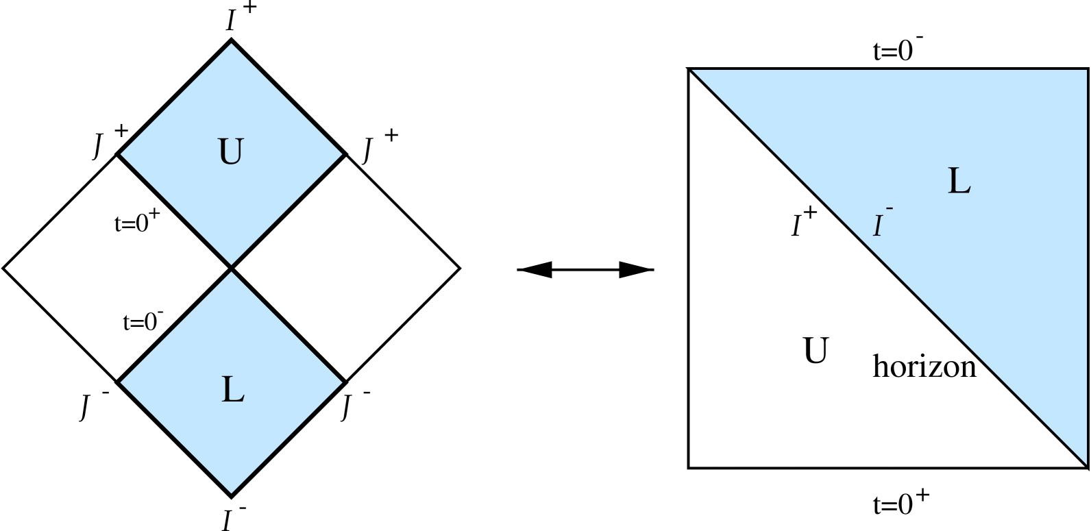
Figure 5: The Milne spacetime is both locally flat (left diagram) and conformally $S^{1}\times$ de Sitter (right diagram, with the 5th dimension suppressed). In the de Sitter picture passing through the singularity corresponds to matching future timelike infinity in de Sitter to past timelike infinity.

A peculiarity of this map is that the collapsing region $L$ of the Milne geometry is mapped to the expanding region $L$ of de Sitter space. Nevertheless the arrow of time always points in the direction of increasing $t$.

De Sitter space can also be globally covered by the closed slicing co-ordinates, so-called because the Cauchy surfaces are spheres $S^{d-1}$. If $d^{2}\Omega_{S^{d-1}}$ denotes the metric on an $S^{d-1}$ with radius $H_{5}$ then the de Sitter metric is

$$ds^{2}=-d\tau^{2}+\cosh^{2}(H_{5}\tau)d^{2}\Omega_{S^{d-1}}$$ (57)

There is no co-ordinate singularity in these co-ordinates which provide an unambiguous method for matching fields from $\cal{I}^{-}$ to $\cal{I}^{+}$. There exists a unitary operator $U(\tau_{1},\tau_{2})$ which generates time evolution from $\tau_{2}$ to $\tau_{1}$. This operator satisfies the Schrodinger equation

$$i\frac{\partial}{\partial\tau_{1}}U(\tau_{1},\tau_{2})=H(\tau_{1})U(\tau_{1},\tau_{2})$$ (58)

where $H(\tau)$ is the time-dependent Hamiltonian. The $S$ matrix is defined as the unitary operator

$$S=\lim_{\tau_{1}\rightarrow\infty,\tau_{2}\rightarrow-\infty}U(\tau_{1},\tau_{2})=Te^{-i\int_{-\infty}^{\infty}H(\tau)d\tau},$$ (59)

which in the Milne picture corresponds to an $S$ matrix matching from $t=0^{+}$ to $t=0^{-}$ or equivalently,

$$|\psi,t=0^{+}>=S^{\dagger}|\psi,t=0^{-}>$$ (60)

Free field theory on de Sitter spacetime therefore provides us with yet another matching prescription for Milne spacetime.

Since the spacetime ${\cal{M_{C}}}\times R^{d-1}$ is locally flat then a massless minimally coupled scalar field is identical to a massless conformally coupled scalar field. In $d+1$ dimensions the conformal coupling term in the Lagrangian is $-\frac{(d-1)}{8d}R\varphi^{2}$. After a conformal transformation we obtain a massless conformally coupled scalar field on $S^{1}\times dS^{d}$. The Ricci scalar on $S^{1}\times dS^{d}$ is simply a constant $R=d(d-1)H_{5}^{2}$ which means we may reinterpret the scalar field as a minimally coupled scalar field with mass $m^{2}=(d-1)^{2}H_{5}^{2}/4$. On Kaluza-Klein compactification over the $S^{1}$ we obtain a tower of scalar fields on $dS^{d}$ with masses $m^{2}=(d-1)^{2}H_{5}^{2}/4+(2\pi n/L)^{2}$.

As we explained earlier the KK zero mode of a minimally coupled scalar on ${\cal{M_{C}}}\times R^{d-1}$ is identical to a minimally coupled scalar on the lower dimensional Einstein frame geometry. This in turn is equivalent to a scalar field of mass $m^{2}=(d-1)^{2}H_{5}^{2}/4$ on $dS^{d}$. This result would seem surprising had we not used the higher dimensional geometry since although the $d$ dimensional geometry is conformal to $dS^{d}$, a minimally coupled scalar field is not conformally invariant.

In de Sitter space there is a one-parameter family of de Sitter invariant vacua[20]. A unique choice, known as the Bunch-Davies vacuum[19], is obtained if we also demand that the Feynman propagator be of the Hadamard form (see Appendix 2). A de Sitter invariant measure of the distance between two points is provided by the variable $z=1+((t-t^{\prime})^{2}-(\vec{x}-\vec{x}^{\prime})^{2})/2tt^{\prime}$. Although we have expressed it in terms of flat slicing co-ordinates, $z$ is globally defined and has the same definition regardless of which patch $t$ and $t^{\prime}$ are in. This means that the Feynman propagator in the Bunch-Davies vacuum can be defined globally in terms of the hypergeometric function[19]

$$G_{F}=H_{5}^{2}\frac{\Gamma((d-1)/2+\nu)\Gamma((d-1)/2-\nu)}{8\pi^{2}}{}_{2}F_{1}[(d-1)/2-\nu,(d-1)/2+\nu;2,\frac{1}{2}(1+z-i\epsilon)]$$ (61)

where $\nu$ depends on the Kaluza-Klein mode number $n$, $\nu=2\pi in/H_{5}L$.

We are interested in calculating the $S$ matrix to determine the matching condition implied by the above propagator. At the free field level it is sufficient to consider how a single particle state evolves. The Feynman propagator allows us to evolve the positive frequency part of a scalar field from one Cauchy surface $t^{\prime}=$ constant, to any point in its causal future,

$$\varphi^{+}(x,t)=i\int d^{d-1}\vec{x}^{\prime}(Ht^{\prime})^{-d}G_{F}(x,t;x^{\prime},t^{\prime})(\overrightarrow{\partial_{t^{\prime}}}-\overleftarrow{\partial_{t^{\prime}}})\varphi^{+}(x^{\prime},t^{\prime})$$ (62)

A simple calculation shows that a positive frequency WKB in state in the region $t\rightarrow+\infty$ evolves to a positive frequency WKB state in the region $t\rightarrow-\infty$. The reason for this can be seen immediately from the conformal diagram since $\cal{I^{+}}$ and $\cal{I^{-}}$ are identified as the same coordinate horizon.

This result can be understood more clearly by realizing that in analogy with Minkowski, we can define particles in de Sitter as representations of the de Sitter group. Since these representations are globally defined and we choose a vacuum that respects the de Sitter symmetry, then it is clear that in the absence of interactions there can be no particle creation in de Sitter spacetime.

At this point we should make clear that this is not in contradiction with the usual statement that there is a thermal distribution of particles in de Sitter space. This description arises because of a different definition of particles, one which is more appropriate to the static patch surrounding an observer’s world-line. The definition of particles in a curved spacetime is observer dependent, but the evolution of fields is observer-independent The Bunch-Davies vacuum is the vacuum in which globally there is no particle creation according to the representation theory definition, but where locally an observer sees a thermal bath of particles.

In conclusion we have reached the same results as before for free field theory, using the de Sitter picture. When one includes interactions, a careful track of the non-minimal couplings must be taken into account. For instance $\lambda\varphi^{4}$ theory in the 4d Einstein frame geometry will correspond to massive $\lambda^{\prime}(t)\varphi^{4}$ theory on de Sitter where $\lambda^{\prime}(t)$ is a new time-dependent coupling constant. Ultimately, it is not clear to us that the Milne-de Sitter correspondence be a useful guide, because the problem of string theory on de Sitter space is probably a harder problem than that of string theory on the Milne spacetime.

IX Conclusion

In this paper we have shown that it is possible to define free quantum fields on the compactified Milne universe in a consistent and unambiguous manner. We have made limited progress in studying interactions, and how these lead to particle production. The density of particles produced at fixed external momentum is finite at tree level. The integrated density was also found to be finite provided the dilaton dependence of couplings caused them to vanish sufficiently rapidly with $t$. We suggested how an adiabatic limit, in which particle production would be exponentially small for small $H_{5}L$, might emerge in string theory. We also pointed out connections with quantum field theory on de Sitter spacetime, which may well be interesting in their own right.

Certainly, much remains to be done to explore quantum fields on the Milne and compactified Milne universe. The methods used here could be extended to include gravitational backreaction, at least for linearised gravity, to follow cosmological perturbations through the singularity. We shall report on a study of loop diagrams for scalar field interactions on ${\cal M}_{C}$ in the near future. A major challenge remaining is to extend these ideas to string theory and M theory.

Acknowledgements: We thank Martin Bucher, Ruth Durrer, Steven Gratton, David Gross, James Hartle, Stephen Hawking, Joe Polchinski, Fernando Quevedo, Nati Seiberg, Paul Steinhardt, Gabriele Veneziano and Toby Wiseman for many useful discussions. AJT acknowledges the support of an EPSRC studentship. The work of NT is supported by PPARC (UK).

Note Added: Since this article was submitted to the archive a number of related articles condisidering fields/strings on backgrounds with cosmological singularities have appeared[21].

X Appendix 1: The Relationship between Canonical and Bogoliubov Transformations

The group of Bogoliubov transformations is identical to the group of linear canonical transformations. For a 2 dimensional phase space these form the group $Sp(2)$, ie those $2\times 2$ matrices that satisfy

$$A^{T}\Omega A=\Omega,$$ (63)

where $\Omega=\left(\begin{array}[]{cc}0&-1\\ 1&0\\ \end{array}\right)$. $Sp(2)$ is a real form of $SU(2)$ and consequently we can write any generator $A$ in terms of the Pauli matrices $\sigma_{\pm}=\frac{1}{2}(\sigma_{1}\pm\sigma_{2})$, $\sigma_{3}$.

$$A=A_{+}(a)A_{-}(b)A_{3}(c)=e^{a\sigma_{+}}e^{b\sigma_{-}}e^{c\sigma_{3}}$$ (64)

If $\left(\begin{array}[]{cc}q\\ p\\ \end{array}\right)$ denotes an arbitrary vector in phase space then the transformed vector $\left(\begin{array}[]{cc}q^{\prime}\\ p^{\prime}\\ \end{array}\right)=A\left(\begin{array}[]{cc}q\\ p\\ \end{array}\right)$ is given by

$$A_{+}\left(\begin{array}[]{cc}q\\ p\\ \end{array}\right)=\left(\begin{array}[]{cc}q+ap\\ p\\ \end{array}\right)$$ (69)

$$A_{-}\left(\begin{array}[]{cc}q\\ p\\ \end{array}\right)=\left(\begin{array}[]{cc}q\\ p+bq\\ \end{array}\right)$$ (74)

$$A_{3}\left(\begin{array}[]{cc}q\\ p\\ \end{array}\right)=\left(\begin{array}[]{cc}e^{c}q\\ e^{-c}p\\ \end{array}\right).$$ (79)

In quantum mechanics $q$ and $p$ are replaced by operators $Q$ and $P$ satisfying the Heisenberg algebra

$$[Q,Q]=[P,P]=0,\qquad[Q,P]=i.$$ (80)

The canonical transformations $A_{+}$, $A_{-}$ and $A_{3}$ can be represented by 3 unitary transformations $U_{+}$, $U_{-}$ and $U_{3}$ given by

$$U_{+}(a)=\exp(\frac{1}{2}iaP^{2}),$$

$$U_{-}(b)=\exp(-\frac{1}{2}ibQ^{2}),$$

$$U_{3}(c)=\exp(\frac{1}{2}ic(PQ+QP)).$$

These follow as a simple consequence of the Heisenberg algebra. We can define creation and annihilation operators in the usual way $a=\frac{1}{\sqrt{2}}(Q+iP)$, $a^{\dagger}=\frac{1}{\sqrt{2}}(Q-iP)$ and consequently an arbitrary canonical transformation corresponds to an arbitrary redefinition of $a$ and $a^{\dagger}$, ie. a Bogoliubov transformation.

In field theory an operator valued field can be expressed in terms of creation and annihilation operators as

$$\varphi(x)=\sum_{i}a_{i}\psi_{i}(x)+a_{i}^{\dagger}\psi^{*}_{i}(x)=\sqrt{2}\sum_{i}Q_{i}Re(\psi_{i}(x))-P_{i}Im(\psi_{i}(x))$$ (82)

with $\psi_{i}(x)$ and $\psi^{*}_{i}(x)$ the positive and negative frequency mode functions, normalised according to the Klein-Gordon inner product. It is usual to write a Bogoliubov transformation as a transformation acting on these modes: $\psi^{\prime}_{i}(x)=\alpha\psi_{i}(x)+\beta\psi^{*}_{i}(x)$, which preserves the Klein-Gordon norm if $|\alpha|^{2}-|\beta|^{2}=1.$ Since the field $\varphi(x)$ is invariant under this transformation, the creation and annihilation operators must transform under the inverse Bogoliubov transformation,

$$a^{\prime}_{i} = \alpha^{*}a_{i}-\beta^{*}a^{\dagger}_{i}$$

$$a^{\prime\dagger}_{i} = \alpha a^{\dagger}_{i}-\beta a_{i}.$$ (83)

If we re-write this in terms of coordinates and momenta, then in the above notation, the Boguliubov transformation corresponds to the linear canonical transformation on the operators $(Q_{i},P_{i})$

$$A=\left(\begin{array}[]{cc}Re(\alpha-\beta)&Im(\alpha+\beta)\\ Im(\beta-\alpha)&Re(\alpha+\beta)\\ \end{array}\right)$$ (84)

It is simple to check that $detA=|\alpha|^{2}-|\beta|^{2}=1$ as required. This formula gives the precise map between canonical transformations and a Bogoliubov transformations.

XI Appendix 2: Hadamard form of the propagator

In the description of quantum fields on a curved spacetime, a natural and common restriction on the choice of vacuum is to impose that the Feynman propagator should be of Hadamard form. More precisely this means that in the coincidence limit $x\rightarrow x^{\prime}$, $G_{F}(x,x^{\prime})$ has the same singularity structure as the Feynman propagator on flat space. A physical motivation for this choice of vacuum is that two observers located at nearby points $x$ and $x^{\prime}$ should not be able to tell if they are on a curved space or Minkowski space by information sent between them. Since we are considering the coincidence limit $x\rightarrow x^{\prime}$ the distinction between the various types of Green’s functions is not relevant and it is common to work exclusively with the Hadamard function defined by

$$G_{H}(x,x^{\prime})=G^{+}(x,x^{\prime})+G^{-}(x,x^{\prime})=-2{\rm Im}G_{F}(x,x^{\prime}),$$ (85)

where $G^{+}(x,x^{\prime})$ denotes the Wightman function $<0|\varphi(x)\varphi(x^{\prime})|0>$ and $G^{-}(x,x^{\prime})$ is its complex conjugate. Now suppose we are interested in the Green’s functions on a spacetime which is invariant under the discrete symmetries of time reversal $T$ and parity $P$. This is true of all the spacetimes we have considered which can be seen by a simple inspection of their metrics. In particular then the spacetimes are invariant under the combined symmetries $PT$. This operator is anti-unitary and modes $\psi_{i}(x)$ may be decomposed into its eigenstates, which with an appropriate choice of phase can be chosen to obey

$$\psi(PTx)=\psi^{*}(x).$$ (86)

Given one such eigenstate, let us construct an arbitrary momentum-independent Bogoliubov transformation, to the mode function

$$\psi^{\prime}(x)=\alpha\psi(x)+\beta\psi^{*}(x).$$ (87)

Then we find that

$$\psi^{\prime}(PTx)=\alpha\psi^{*}(x)+\beta\psi(x).$$ (88)

If we demand that $\psi^{\prime}(x)$ also be an eigenstate of $PT$ with eigenvalue $\eta$ (which can be an arbitrary complex phase), then we must have

$$\alpha^{*}=\eta\alpha,\beta^{*}=\eta\beta,$$ (89)

relations which can only be satisfied if Im$(\alpha\beta^{*})$ is zero, a result we shall use in a moment.

Given a particular set of positive frequency modes $\psi_{i}(x)$ which are time reversal invariant $\psi_{i}(PTx)=\psi_{i}(x)^{*}$ and for which the vacuum is Hadamard we can construct the Hadamard function as,

$$G_{H}(x,x^{\prime})=\sum_{i}\psi_{i}(x)\psi^{*}_{i}(x^{\prime})+c.c.$$ (90)

Now define a new vacuum by means of a constant Bogoliubov transformation of the first vacuum

$$\psi^{\prime}_{i}(x)=\alpha\psi_{i}(x)+\beta\psi_{i}^{*}(x).$$ (91)

The Hadamard function in the new vacuum is given by

$${G}^{\prime}_{H}(x,x^{\prime})=(|\alpha|^{2}+|\beta|^{2})G_{H}(x,x^{\prime})+2Re(\alpha\beta^{*})G_{H}(x,PTx^{\prime})-2Im(\alpha\beta^{*})\Delta(x,PTx^{\prime})$$

The commutator function

$$[\varphi(x),\varphi(x^{\prime})]=G^{+}(x,x^{\prime})-G^{-}(x,x^{\prime})=i\Delta(x,x^{\prime})$$ (92)

does not contribute to the Hadamard singularity structure since it is vacuum independent. The singularity of $\Delta(x,x^{\prime})$ occurs for null separated points only. However, the commutator ${G}^{\prime}_{H}(x,x^{\prime})$ in the new vacuum will have singular behaviour in the coincidence limit $x^{\prime}\rightarrow PTx$. But one of the requirements of the Hadamard vacuum is that the propagator only has a singularity as $x\rightarrow x^{\prime}$. Consequently if we demand that the new vacuum is Hadamard then we must have Re$(\alpha\beta^{*})=0$.

The conditions derived in the previous two paragraphs together imply that $\beta=0$. In other words, the requirement of $PT$ invariance and Hadamard form uniquely picks out the vacuum. In fact all the vacua we have considered in this paper are trivially $P$ invariant, $G^{+}(Px,Px^{\prime})=G^{+}(x,x^{\prime})$, and so we only need to additionally impose the restriction of $T$ invariance.

To put this in the more familiar setting of quantum fields on de Sitter space, the condition that the vacuum propagator be de Sitter invariant automatically picks out a vacuum invariant under $PT$ since $PT$ is a discrete subgroup of the full de Sitter symmetry. Then, as is well known, the additional requirement of Hadamard form uniquely picks the vacuum as the standard Euclidean, or Bunch-Davies vacuum.

References

- [1] L.J. Dixon, J.A. Harvey, C.Vafa and E. Witten, Nuc. Phys. B261, (1985) 678, Nuc. Phys. B274, (1986) 285.
- [2] P.S. Aspinwall, B.R. Greene and D.R. Morrison, Nucl. Phys. B416 (1994) 414; E. Witten, Nucl. Phys. B403 (1993) 159.
- [3] J. Khoury, B.A. Ovrut, P.J. Steinhardt and N. Turok, hep-th/0103239, Phys.Rev. D64 (2001) 123522.
- [4] P.J. Steinhardt and N. Turok, hep-th/0111030, Science, May 24 (2002) 1436; Phys. Rev. D64 (2002) 126003.
- [5] G. Veneziano, Phys. Lett. B265 (1991) 287; M. Gasperini and G. Veneziano, Astropart. Phys. 1 (1993) 317; for a review see G. Veneziano, hep-th/0002094.
- [6] J. Khoury, B.A. Ovrut, N. Seiberg, P.J. Steinhardt and N. Turok, Phys. Rev. D65 (2002) 086007; N. Seiberg, hep-th/0201039.
- [7] D.H. Lyth, Phys. Lett. B524 (2002) 1; ibid. B526 (2002) 173; R. Brandenberger and F. Finelli, JHEP 0111 (2001) 056; F. Finelli and R. Brandenberger, Phys. Rev. D65 (2002) 103522 ; J-C. Hwang, Phys. Rev. D65 (2002) 063514 ; J-C. Hwang and H. Noh, Phys. Rev. D65 (2002) 124010 ; J. Martin, P. Peter, N. Pinto-Nieto and D.J. Schwarz, Phys. Rev. D65 (2002) 123513.
- [8] J. Khoury, B.A. Ovrut, P.J. Steinhardt and N. Turok, hep-th/0109050, Phys. Rev. D, in press.
- [9] R. Durrer, hep-th/0112026; R. Durrer and F. Vernizzi, hep-ph/0203275.
- [10] P. Peter and N. Pinto-Nieto, hep-th/0203013.
- [11] G. Horowitz and A. Steif, Phys. Lett. B258 (1991) 91.
- [12] See e.g. T. Banks, hep-th/9911067.
- [13] R. Bousso, hep-th/0203101, Rev. Mod. Phys., in press (2002).
- [14] A. Strominger, hep-th/0106113, JHEP 0110 (2001) 034.
- [15] V. Balasubramanian, S.F. Hassan, E. Keski-Vakkuri, A. Naqvi, hep-th/0202187.
- [16] N. Nekrasov, hep-th/0203112.
- [17] L. Cornalba and M.S. Costa, hep-th/0203031.
- [18] D.M. Chitre and J.B. Hartle, Phys.Rev. D16 (1977) 251.
- [19] N.D. Birrell and P.C. Davies, Quantum fields in curved space, CUP.
- [20] B. Allen, A. Folacci, Phys. Rev. D35 (1987) 3771.
- [21] L. Cornalba, M.S. Costa, C. Kounnas, hep-th/0204261; B. Craps, D. Kutasov, G. Rajesh, hep-th/0205101; H. Liu, G. Moore, N. Seiberg, hep-th/0206182; G.T. Horowitz, J. Polchinski, hep-th/0206228; M. Fabinger, J. McGreevy, hep-th/0206196; S. Elitzur, A. Giveon, D. Kutasov, E. Rubinovic, hep-th/0204189.