Open Strings

Abstract

This review is devoted to open strings, and in particular to the often surprising features of their spectra. It follows and summarizes developments that took place mainly at the University of Rome “Tor Vergata” over the last decade, and centred on world-sheet aspects of the constructions now commonly referred to as “orientifolds”. Our presentation aims to bridge the gap between the world-sheet analysis, that first exhibited many of the novel features of these systems, and their geometric description in terms of extended objects, D-branes and O-planes, contributed by many other colleagues, and most notably by J. Polchinski. We therefore proceed through a number of prototype examples, starting from the bosonic string and moving on to ten-dimensional fermionic strings and their toroidal and orbifold compactifications, in an attempt to guide the reader in a self-contained journey to the more recent developments related to the breaking of supersymmetry.

CERN-TH/2002-025

ROM2F-2002/08

LPTENS 02/14

CPHT RR 020.0202

hep-th/0204089

Dedicated to John H. Schwarz
on the occasion of his sixtieth birthday

1 Introduction and summary

The celebrated Veneziano formula [1] for open-string tachyons, that marked the birth of String Theory in the form of “dual models” for hadron resonances, was shortly followed by the Shapiro-Virasoro formula for closed-string tachyons [2] and by their multi-particle generalizations [3], as well as by the Neveu-Schwarz-Ramond fermionic string [4]. The early work of the following decade provided the foundations for the subject [5], whose very scope took a sharp turn toward its current interpretation as a theory of the fundamental interactions only at the end of the seventies, some time after Scherk and Schwarz and Yoneya [6] elucidated the close link between the low-energy behaviour of string amplitudes on the one hand, and higher-dimensional gauge theories and gravity on the other. The work of Green and Schwarz, that finally resulted in their celebrated anomaly cancellation mechanism [7], opened the way to the string construction of four-dimensional chiral spectra free of the usual ultraviolet divergences of point-particle gravity [8]. This originally rested on Calabi-Yau compactifications [9, 10] of the low-energy supergravity [11] of heterotic strings [12], that for many years have been at the heart of string phenomenology. Most of the efforts were then related to the ${\rm E}_{8}\times{\rm E}_{8}$ heterotic model, naturally connected to four-dimensional low-energy physics, and it was indeed the prominence of exceptional gauge groups [13], generated by charges spread over closed strings [14], together with the impossibility of realizing them in open strings [15, 16, 17], that stimulated this intense activity [18]. The seminal work of Gliozzi, Scherk and Olive (GSO) [19] somehow laid the ground for a string description of these phenomena, since it first showed how a naïve string spectrum could be naturally projected to a supersymmetric one. Why these projections should generally be present, however, became clear only in the late eighties, when they were given a raison d’être in the geometric constraint of modular invariance [20] of the underlying conformal field theory [21, 22, 23], a property that the bosonic string had manifested long before [24]. By then, one had attained a precise dictionary relating world-sheet constructions to their space-time counterparts, albeit limitedly to the case of oriented closed strings, and some of these could be related, via suitable compactifications, to chiral four-dimensional matter coupled to ${\cal N}=1$ supergravity [25, 26, 27]. A basic entry in this respect was provided by the idea of orbifolds [28], that not only allowed to extend string constructions beyond the toroidal case [29] but, more importantly, endowed a wide class of GSO projections with a geometric interpretation, linking them to singular limits of Calabi-Yau reductions. Discrete symmetries play a pivotal rôle in this context, while the orbifold structure permeates the whole of Conformal Field Theory [23].

The work of the “Tor Vergata” group summarized in this review began in the second half of the eighties. The realization of consistent GSO projections for open strings then emerged as a major open problem, since standard ideas based on modular invariance failed to apply directly to world sheets with boundaries. The main insights were provided by the absence of short-distance singularities in the SO(32) superstring [30], ultimately responsible for its anomaly cancellation, and by a similar behaviour of the SO(8192) bosonic string. This had been exhibited by three rather distinct methods: direct calculation of one-point functions [31], factorization of tachyon amplitudes [32] and singular limits of vacuum amplitudes [33, 34]. The difference between the two types of phenomena was elucidated in [35], where the absence of space-time anomalies in the SO(32) superstring was related to the behaviour of its R-R sector. In both cases, however, one knew neither how to break the gauge group, nor how to attain any non-trivial compactification. Orbifolds provided again the proper setting, once extended to discrete symmetries mixing left and right modes [36], and this generalization, now commonly termed an “orientifold”, linked the closed and open bosonic strings in twenty-six dimensions and the type I and type IIB superstrings in ten dimensions.

A few other groups [37, 38] soon elaborated on the proposal of [36], while others were considering similar issues from an apparently different viewpoint. Their work marked the birth of D-branes, that emerged from the behaviour under T-duality of open-string toroidal backgrounds [39, 40, 41]. These also made an early appearance in [42], in an analysis of $\hbox{\mbm Z}_{2}$ orbifolds stimulated by the low-energy considerations in [43], but the emphasis fell solely on their spectrum that, however, clearly revealed the rôle of Neumann-Neumann, Neumann-Dirichlet and Dirichlet-Dirichlet strings and their mutual consistency. Once more, the basic ingredients were long known [44], while the novelties were the rules enforcing the proper GSO projections. Our later efforts [45] were stimulated by the fermionic constructions of four-dimensional superstrings [25, 26] and by related properties of lattices [27], in an attempt to constrain the GSO projections from the residual higher-loop modular invariance, but soon the seminal paper of Cardy on Boundary Conformal Field Theory [46] allowed a precise algebraic construction of boundaries respecting a given symmetry [47, 48]. This promptly resulted in new classes of ten-dimensional orientifolds, the 0A and 0B descendants, with rich patterns of gauge symmetry, and in new surprising six-dimensional models with (1,0) supersymmetry that, in sharp contrast with heterotic ones, contain variable numbers of (anti)self-dual two-forms. Their presence was an early success for the proposal of [36], as we soon realized [49], since the two-forms, remnants of the 21 type IIB ones of the $T^{4}/\hbox{\mbm Z}_{2}$ orbifold, play a crucial rôle in a generalized version of the Green-Schwarz anomaly cancellation mechanism. The six-dimensional supergravity models associated to these generalized Green-Schwarz terms are also of interest in their own right, since they display singularities in the gauge couplings, first noticed in [49], that can be associated to a novel type of phase transition whereby a soliton of the model, a string, becomes tensionless [50]. Six-dimensional string models obtained from compactifications on group lattices also exhibited peculiar rank reductions of the Chan-Paton gauge group, that could be linked to quantized values of the NS-NS two-form $B_{ab}$ [51, 52, 53]. Our subsequent efforts were aimed at a better understanding of the underlying boundary (and crosscap) Conformal Field Theory, first in diagonal minimal models [54], where the Cardy prescription was extended to the Klein bottle and Möbius amplitudes, and then in WZW models, where new structures emerged and, perhaps more importantly, where we learned how to modify Klein-bottle projections [55, 56, 57]. This soon resulted in an interesting application: a ten-dimensional 0B orientifold completely free of tachyons, now commonly termed $0^{\prime}{\rm B}$ string [58, 59, 60, 61].

Polchinski’s paper on the R-R charge of D-branes and O-planes [62] gave rise to an upsurge of interest in these constructions, as well as in the rôle of open strings in non-perturbative aspects of closed-string physics, since it tied a number of world-sheet results to a pervasive space-time picture involving solitonic extended objects, with a key rôle in the web of string dualities [63] . Many started working actively on D-branes and orientifolds, and new developments followed. Our work summarized here has led to the first instance of a four-dimensional model with three generations of chiral matter [64], the starting point for a number of subsequent constructions [65], to a better understanding of the peculiar current algebra associated to the generalized Green-Schwarz mechanism [66] and, more recently, to novel realizations of supersymmetry breaking by Scherk-Schwarz deformations [67] in string vacua allowed by the presence of open strings [68, 69, 70, 71] and by the simultaneous presence of branes and antibranes [72, 73, 74, 75]. This work extended the original closed-string constructions of [76] to the case of open strings, exhibiting the new phenomenon of “brane supersymmetry breaking” [77, 53, 73, 78, 74, 75], met independently in the USp(32) ten-dimensional type I model in [79]. More recently, stimulated by the proposal of [80, 81] on magnetic supersymmetry breaking, we have also studied instanton-like [83] magnetic deformations yielding new supersymmetric vacua with gauge groups of reduced rank and multiple matter sectors [84, 85]. These constructions may be regarded as a realization in type I vacua of proposals related to systems of branes at angles [86], a viewpoint widely pursued by other groups in attempts to construct brane realizations of the Standard Model [87].

In writing this review, we have made a selection of the topics that we have touched upon over the years, in an attempt to guide the reader, hopefully in a self-contained and pedagogical fashion, through a number of examples, drawn mostly from toroidal and orbifold models, that are meant to illustrate the wide variety of phenomena brought about by these generalized GSO projections in their simplest occurrences. As a result, our discussion is centred on the key features of the open-string partition functions and of the underlying Boundary Conformal Field Theory, at the expense of other interesting topics, to wit the low-energy effective field theory and the applications to model building, that are left out. We thus begin with the bosonic string and its orientifolds, and proceed to ten-dimensional fermionic strings and their toroidal and orbifold compactifications, with a slight diversion at the end to display some general properties of the D-branes allowed in the ten-dimensional string models. The concluding section highlights some general aspects of (rational) Boundary Conformal Field Theory, showing in particular how orientifolds can also prove useful tools to extract D-brane spectra and how one can formulate “completeness” conditions [57] for boundaries or, equivalently, for brane types. We shall emphasize throughout how the partition functions of abstract Conformal Field Theories, even beyond their applications to String Theory, if properly formulated, encode clearly all relevant phenomena. The review of Dudas [88] on phenomenological aspects of type I vacua and the more recent review of Stanev [89] on Boundary Conformal Field Theory have some overlap, both in spirit and in contents, with the present one, while a number of previous short reviews have also touched upon some of these issues [90].

It is a pleasure to dedicate this review article to John H. Schwarz on the occasion of his sixtieth birthday. His work pervades the whole of String Theory, and in particular the developments summarized here, while his example inspired, directly or indirectly, both us and our friends and collaborators educated at the University of Rome “Tor Vergata”.

2 The bosonic string

In this section we describe some generic features of open-string constructions, using the bosonic string as an example. In particular, we review the basic structure of the Polyakov expansion and some general properties of Chan-Paton groups, including their relation to fermionic modes living at the ends of open strings. We shall confine our attention to the light-cone quantization method, sufficient to describe string spectra in most circumstances. Here we shall meet the four vacuum amplitudes with vanishing Euler character that determine the spectrum of these models: torus, Klein bottle, annulus and Möbius strip. Finally, in this simple setting we shall also make our first encounter with a tadpole condition, that determines a special choice for the open-string gauge group.

2.1 The Polyakov expansion

Models of oriented closed strings have the simple and remarkable feature of receiving one contribution at each order of perturbation theory [91]. These correspond to closed orientable Riemann surfaces with increasing numbers of handles $h$ [92], and their perturbative series is weighted by $g_{s}^{-\chi}$, where the Euler character $\chi$ is

$$\chi=2-2h\,,$$ (1)

and where the string coupling $g_{s}$ is determined by the vacuum expectation value of a ubiquitous massless scalar mode of closed strings, the dilaton $\varphi$, according to

$$g_{s}=e^{\langle\varphi\rangle}\,.$$ (2)

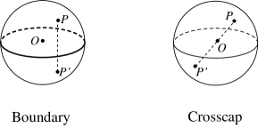
Figure 1: Boundary and crosscap.

The models of interest in this review are actually more complicated. Their closed strings are unoriented, while their spectra usually include additional sectors with unoriented open strings. As a result, their Polyakov expansions involve additional Riemann surfaces, that contain variable numbers of two new structures: holes surrounded by boundaries, $b$, and crosscaps, $c$ [93]. The Euler character for a surface with $h$ handles, $b$ holes and $c$ crosscaps is

$$\chi=2-2h-b-c\,,$$ (3)

and therefore the perturbation series now includes both even and odd powers of $g_{s}$. Boundaries are easily pictured, and their simplest occurrence is found in a surface of Euler character $\chi=1$, the disk. This is doubly covered by a sphere, from which it may be retrieved identifying pair-wise points of opposite latitude, as in figure 1. The upper hemisphere then corresponds to the interior of the disk, while the equator, a line of fixed points in this construction, defines its boundary. On the other hand, crosscaps are certainly less familiar. Still, their simplest occurrence is found in another surface of Euler character $\chi=1$, the real projective plane, obtained from a sphere identifying antipodal points, as in figure 1. One can again take as a fundamental region the upper hemisphere, but now pairs of points oppositely located on the equator are identified. In loose terms, we shall call such a line, responsible for the lack of orientability of this surface, a crosscap. As can be seen from figure 1, the end result is a closed non-orientable surface, where the transport of a pair of axes can reverse their relative orientation.

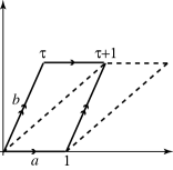
Figure 2: The torus as a periodic lattice.

In general, all these surfaces may be dissected and opened on the plane by a suitable number of cuts, and for surfaces of vanishing Euler character the plane can be equipped with a Euclidean metric. Thus, for instance, two cuts turn a torus into the parallelogram of figure 2, whose opposite sides are to be identified as indicated by the arrows. By a suitable rescaling, one of the sides may be chosen horizontal and of length one, and thus a single complex number, $\tau=\tau_{1}+i\tau_{2}$, with positive imaginary part $\tau_{2}$, usually called the Teichmüller parameter, or modulus for brevity, defines the shape or, more precisely, the complex structure of this surface. There is actually a subtlety, since not all values of $\tau$ in the upper-half complex plane correspond to inequivalent tori. Rather, all values related by the ${\rm PSL}(2,\hbox{\mbm Z})={\rm SL}(2,\hbox{\mbm Z})/\hbox{\mbm Z}_{2}$ modular group, that acts on $\tau$ according to

$$\tau\to\frac{a\tau+b}{c\tau+d}\qquad{\rm with}\qquad ad-bc=1\,,\quad a,b,c,d\in\hbox{\mbm Z}\,,$$ (4)

are to be regarded as equivalent. This group is generated by the two transformations

$$T:\tau\to\tau+1\,,\qquad S:\tau\to-\frac{1}{\tau}\,,$$ (5)

that in SL(2,ℤ) satisfy the relation

$$S^{2}=(ST)^{3}\,.$$ (6)

Notice that $T$ redefines the oblique side of the fundamental cell, while $S$ interchanges horizontal and oblique sides. As a result, the independent values of $\tau$ lie within a fundamental region of the modular group, for instance within

$${\cal F}=\{-{\textstyle{1\over 2}}<\tau_{1}\leq{\textstyle{1\over 2}},|\tau|\geq 1\}$$ (7)

of figure 3. This property and its generalizations to other surfaces play a crucial rôle in the construction of string models.

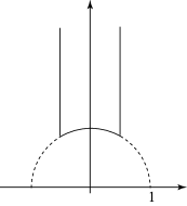
Figure 3: Fundamental domain for the torus.

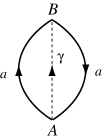
Figure 4: A non-contractible loop $\gamma$ and the crosscap.

In a similar spirit, one can unfold the projective plane into the region of figure 4, where the two sides are again to be identified according to the arrows, and the additional dashed line $\gamma$ suffices to reveal a peculiar property of this surface. To this end, let us imagine to move along $\gamma$ from a point $A$ to its opposite image $B$, a closed path that is clearly not contractible. However, moving $\gamma$ across one of the two vertical sides of the polygon has the net effect of reversing its orientation and, as a result, while $\gamma$ is non contractible, $\gamma^{2}$ is, as can be seen reversing the orientation of one of the two copies. This illustrates a familiar result: the fundamental group of the real projective plane is $\hbox{\mbm Z}_{2}$ [94].

It is simple to extract the fundamental group of a surface from the corresponding polygon [94], associating a generator, or its inverse, to each independent side, according to the clockwise or counter-clockwise orientation of the corresponding arrows. These generators are not independent, however, since the interior of the polygon is clearly contractible, and as a result one has a relation. For instance, for the torus of figure 2 one finds $b^{-1}a^{-1}ba=1$, and the resulting fundamental group is thus Abelian, since its two generators $a$ and $b$ commute. In a similar fashion, for the projective disk this leads to the condition $a^{2}=1$, so that, as previously stated, in this case there is a non-trivial $\hbox{\mbm Z}_{2}$ generator.

There are four surfaces with vanishing Euler character. Leaving aside the torus, that we have already discussed, $\chi=0$ can indeed be obtained for three other choices: the Klein bottle ($h=0$, $b=0$, $c=2$), the annulus ($h=0$, $b=2$, $c=0$) and the Möbius strip ($h=0$, $b=1$, $c=1$).

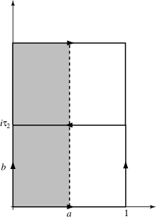
Figure 5: Fundamental polygons for the Klein bottle.

Like the projective disk, the Klein bottle has the curious feature of not allowing an embedding in three-dimensional Euclidean space that is free of self-intersections. Two choices for the corresponding polygon, together with one for the doubly-covering torus, are shown in figure 5. The first polygon, of sides 1 and $i\tau_{2}$, presents two main differences with respect to the torus of figure 2: the horizontal sides have opposite orientations, while $\tau$ is now purely imaginary. The Klein bottle can be obtained from its covering torus, of Teichmüller parameter $2i\tau_{2}$, if the lattice translations are supplemented by the anticonformal involution

$$z\to 1-\bar{z}+i{\tau_{2}}\,,$$ (8)

where the “vertical” time $\tau_{2}$ is the “proper world-sheet time” elapsed while a closed string sweeps it. The second choice of polygon, also quite interesting, defines an inequivalent “horizontal” time. It is obtained halving the horizontal side while doubling the vertical one, and thus leaving the area unaltered. The end result has the virtue of displaying an equivalent representation of this surface as a tube terminating at two crosscaps, and the horizontal side is now the “proper time” elapsed while a closed string propagates between the two crosscaps. The tube is the interior of the region, whose horizontal sides have now the same orientation, while the crosscaps are the two vertical sides, where points differing by translations by half of their lengths are pair-wise identified. It should also be appreciated that, in moving from the first fundamental polygon to the double cover, the identifications are governed by eq. (8), that has no fixed points and squares to the vertical translation $z\to z+2i\tau_{2}$. Finally, the corresponding relation for the generators of the fundamental group,

$$b^{-1}a^{-1}ba^{-1}=1\,,$$ (9)

implies that $a$ and $a^{-1}$ belong to the same conjugacy class, a result that will have a direct bearing on the ensuing discussion.

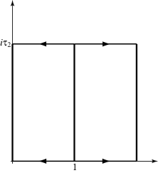
Figure 6: Fundamental polygon for the annulus.

The annulus is certainly more familiar. Its fundamental polygon is displayed in figure 6, together with a polygon for its doubly-covering torus, obtained by horizontal doubling. In the original polygon, with vertices at 1 and $i\tau_{2}$, the horizontal sides are identified, while the vertical ones correspond to the two boundaries. These are fixed-point sets of the involutions

$$z\to-\bar{z}\qquad{\rm and}\qquad z\to 2-\bar{z}$$ (10)

that recover the annulus from the doubly-covering torus. Once more, $\tau$ is purely imaginary, and $\tau_{2}$ is now the “proper time” elapsed while an open string sweeps the annulus. One has again a distinct “horizontal” choice, that defines the “proper time” elapsed while a closed string propagates between the two boundaries.

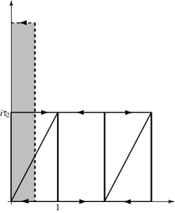
Figure 7: Fundamental polygons for the Möbius strip.

Finally, the Möbius strip corresponds to the polygon in figure 7, again with vertices at 1 and $i\tau_{2}$, but whose horizontal sides have opposite orientations. It should be appreciated that now the vertical sides describe two different portions of a single boundary. The parameter $\tau_{2}$ describes the “proper time” elapsed while an open string sweeps the Möbius strip, and one has again the option of choosing a different fundamental polygon, that displays an equivalent representation of the surface as a tube terminating at one hole and one crosscap. This is simply obtained doubling the vertical side while halving the horizontal one. One of the two resulting vertical sides is the single boundary of the Möbius strip, while the other, where points are pair-wise identified after a vertical translation on account of the involution

$$z\to 1-\bar{z}+i\tau_{2}\,,$$ (11)

is the crosscap, and the corresponding horizontal time defines the “proper time” elapsed while a closed string propagates between the boundary and the crosscap. It should be appreciated that in this case the polygon obtained doubling the vertical length defines an annulus, not a torus. A doubly-covering torus does exist, of course, but has the curious feature of having a Teichmüller parameter that is not purely imaginary. This may be seen combining the anticonformal involution of eq. (11) with eq. (10), that identifies the boundary of the Möbius strip. Referring to figure 7, horizontal and skew sides are now consistently identified, but

$$\tau={\textstyle\frac{1}{2}}+{\textstyle{1\over 2}}i\tau_{2}\,,$$ (12)

after rescaling to one the length of the horizontal side.

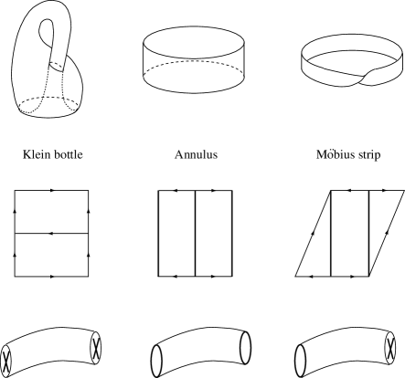
Figure 8: Klein bottle, annulus and Möbius strip.

It is time to summarize these results. Whereas for the torus one has an infinity of equivalent choices for the “proper time”, that reflect themselves into the invariance under the modular group ${\rm SL}(2,\hbox{\mbm Z})$, each of the other three surfaces allows two inequivalent canonical choices, naïvely related by an $S$ modular transformation. One of these choices, corresponding to the “vertical” time, exhibits the propagation of closed strings in the Klein bottle and of open strings in the other two surfaces. On the other hand, the “horizontal” time exhibits in all three cases the propagation of closed strings between holes and/or crosscaps. There is actually a technical subtlety, introduced by the doubly-covering torus of the Möbius strip, whose Teichmüller parameter, given in eq. (12), is not purely imaginary. Since the string integrand will actually depend on it, one is effectively implementing the transformation [95]

$$P:\ \frac{1}{2}+i\frac{\tau_{2}}{2}\to\frac{1}{2}+i\frac{1}{2\tau_{2}}\,,$$ (13)

that can be obtained by a sequence of $S$ and $T$ transformations, as

$$P=TST^{2}S$$ (14)

and, on account of eq. (6), satisfies

$$P^{2}=S^{2}=(ST)^{3}\,.$$ (15)

This review, being devoted to the study of string spectra, is centred on these surfaces of vanishing Euler character. Still, we would like to conclude the present discussion showing in some detail an important topological equivalence between surfaces of higher genera: one handle and one crosscap may be replaced by three crosscaps [94]. This effectively limits the Polyakov expansion to surfaces with arbitrary numbers of handles $h$ and holes $b$, but with only 0,1 or 2 crosscaps $c$. The simplest setting to exhibit this equivalence is displayed in figure 9, that shows a choice of fundamental polygon, a hexagon, for a surface comprising a crosscap, the sequence of the two $a$ sides, and a handle, the sequence $bcb^{-1}c^{-1}$. One can now prove the equivalence performing a series of cuttings and glueings or, equivalently, moving to different choices for the fundamental polygon. To this end, let us begin by introducing a horizontal cut through the centre of the hexagon, and let $d$ denote the corresponding new pair of sides thus created. We can then move one of the two resulting trapezia and glue the two halves $a$ of the crosscap. The new hexagon contains pairs of sides with clockwise orientations, somewhat reminiscent of the structure of three crosscaps, albeit still separated from one another. Two more cuttings and glueings suffice to exhibit three neighbouring couples. They both remove triangles whose two external sides have opposite orientations, and then join sides that, in the hexagon, have like orientations. Thus, referring to the figure, we now cut out the triangle $be^{-1}d^{-1}$ in the upper left corner and glue the two $b$ sides. In the resulting hexagon the two $e$ sides, next to one another, define one crosscap. Finally, cutting out the triangle $cd^{-1}f^{-1}$ and gluing the two resulting $c$ sides fully exhibits the three crosscaps.

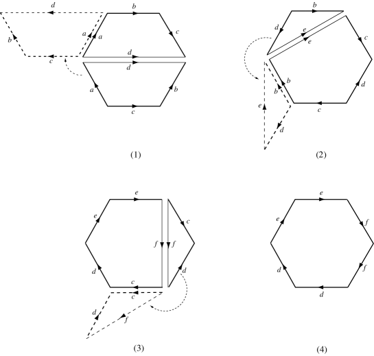
Figure 9: An important equivalence: $3c\equiv h+c$.

2.2 Light-cone quantization

Let us now turn to the quantization of bosonic strings. The starting point is the action for a set of $D$ world-sheet scalars, identified with the string coordinates in a $D$-dimensional Minkowski space-time, coupled to world-sheet gravity [96]. The corresponding action principle is

$$S=-\frac{1}{4\pi\alpha^{\prime}}\int d^{2}\xi\sqrt{-g}g^{\alpha\beta}\partial_{\alpha}X^{\mu}\ \partial_{\beta}X^{\nu}\ \eta_{\mu\nu}+\frac{\langle\varphi\rangle}{4\pi}\int d^{2}\xi\sqrt{-g}R\,,$$ (16)

where we have added an Einstein term, that in this case is a topological invariant, the Euler character of the surface, and a coupling $\langle\varphi\rangle$ whose exponential weights the perturbation series.

One can derive rather simply the spectrum of this model, following [97]. To this end, one can use the field equations for the background metric, i.e. the condition that the energy momentum tensor

$$T_{\alpha\beta}=\partial_{\alpha}X^{\mu}\partial_{\beta}X_{\mu}-{\textstyle\frac{1}{2}}g_{\alpha\beta}\ \partial^{\gamma}X^{\mu}\partial_{\gamma}X_{\mu}$$ (17)

vanish, to express the longitudinal string coordinates in terms of the transverse ones. The procedure, reminiscent of the usual light-cone formulation of Electrodynamics, is quite effective since the string coordinates actually solve

$$\partial_{\alpha}\left(\sqrt{-g}g^{\alpha\beta}\partial_{\beta}\ X^{\mu}\right)=0\,,$$ (18)

that reduces to the standard wave equation

$$\left(\frac{\partial^{2}}{\partial\tau^{2}}-\frac{\partial^{2}}{\partial\sigma^{2}}\right)\ X^{\mu}=0$$ (19)

if a convenient choice of coordinates $\xi^{\alpha}=(\tau,\sigma)$ is used to turn the background metric $g_{\alpha\beta}$ to the diagonal form

$$g_{\alpha\beta}=\Lambda(\xi)\ \eta_{\alpha\beta}\,.$$ (20)

$\Lambda$ then disappears from the classical action (16) and, in the critical dimension $D=26$, that we shall soon recover by a different argument, from the functional measure as well [91]. The longitudinal string coordinates can be eliminated since, even after this gauge fixing, the original invariances under Weyl rescalings and reparametrizations leave behind a residual infinite symmetry that, after a Euclidean rotation, would correspond to arbitrary analytic and antianalytic reparametrizations [5, 21, 22, 23]. This is the case since the string action of eq. (16) effectively describes massless free fields, and is thus a simple instance of a two-dimensional conformally invariant model. The infinite dimensional group of conformal and anticonformal reparametrizations is the basis of two-dimensional Conformal Field Theory [21, 23] that, as we shall review briefly in section 6, provides the very rationale for this case, as well as for more general space-time backgrounds.

Before solving eq. (19) for the simplest case, $D=26$ Minkowski space-time, one need distinguish between two options. A closed line defines a closed string, and in the present, simplest case, calls for the decomposition in periodic modes [5, 10]

$$X^{\mu}=x^{\mu}+2\alpha^{\prime}\,p^{\mu}\ \tau+\frac{i\sqrt{2\alpha^{\prime}}}{2}\ \sum_{n\not=0}\left(\frac{\alpha^{\mu}_{n}}{n}\ e^{-2in(\tau-\sigma)}+\frac{\tilde{\alpha}^{\mu}_{n}}{n}\ e^{-2in(\tau+\sigma)}\right)\,,$$ (21)

consistent with 26-dimensional Lorentz invariance. In a similar fashion, a segment defines an open string, and in the present, simplest case, calls for the Neumann boundary conditions $X^{\prime}=0$ at $\sigma=0,\pi$, and thus for the decomposition [5, 10]

$$X^{\mu}=x^{\mu}+2\alpha^{\prime}\,p^{\mu}\ \tau+i\sqrt{2\alpha^{\prime}}\ \sum_{n\not=0}\frac{\alpha^{\mu}_{n}}{n}\ e^{-in\tau}\cos(n\sigma)\,.$$ (22)

Using the residual symmetry one can now make a further very convenient choice for the string coordinates, the light-cone gauge [97]. Defining $X^{\pm}=(X^{0}\pm X^{D-1})/\sqrt{2}$, this corresponds to eliminating, for both open and closed strings, all oscillations in the ‘$+$’ direction, so that

$$X^{+}=x^{+}+2\alpha^{\prime}\,p^{+}\ \tau\,.$$ (23)

This condition identifies target-space and world-sheet times, and is the analogue, in this context, of the condition $A^{+}=0$ in Electrodynamics. One can then use the constraints to eliminate $X^{-}$, and indeed eq. (17) results in the two conditions

$$2\sqrt{2}\,\alpha^{\prime}\,p^{+}\ \partial_{\pm}X^{-}\ -\ {(\partial_{\pm}X^{i})}^{2}=0\,,$$ (24)

that determine the content of $X^{-}$ in terms of the $X^{i}$’s. The remaining transverse sums define the transverse Virasoro operators

$$L_{m}={\textstyle\frac{1}{2}}\sum_{n}\ {\alpha}_{m-n}^{i}{\alpha}_{n}^{i}\,,$$ (25)

and the corresponding $\bar{L}_{m}$ built out of the $\tilde{\alpha}$ that, on account of eq. (24), define the oscillator modes in the ‘$-$’ direction. The $L_{m}$ and the $\bar{L}_{m}$ are clearly mutually commuting, since they are built out of independent oscillator modes, and only $L_{0}$ and $\bar{L}_{0}$ need proper normal ordering. Furthermore, both the $L_{m}$ and the $\bar{L}_{m}$ satisfy the Virasoro algebra with central charge $c=D-2$:

$$[L_{m},L_{n}]=(m-n)L_{m+n}+\frac{D-2}{12}\ m(m^{2}-1)\delta_{m+n,0}\,.$$ (26)

The zero modes of eq. (24) define the mass-shell conditions for physical states, and for the closed string one thus obtains the two conditions

$$2p^{+}p^{-}=\frac{4}{\alpha^{\prime}}\left(L_{0}-\frac{D-2}{24}\right)=\frac{4}{\alpha^{\prime}}\left(\bar{L}_{0}-\frac{D-2}{24}\right)$$ (27)

or, equivalently,

$$2p^{+}p^{-}=\frac{2}{\alpha^{\prime}}\left(L_{0}+\bar{L}_{0}-\frac{D-2}{12}\right)\,,$$ (28)

together with the “level-matching” condition $L_{0}=\bar{L}_{0}$ for physical states. The constant term may be justified from the normal ordering of the Virasoro operators $L_{0}$ and $\bar{L}_{0}$, identifying the corresponding divergent sums over zero-point energies with a particular value of the Riemann $\zeta$ function, $\zeta(-1)=-\frac{1}{12}$ [98]. This result is a special case of the class of relations

$$\zeta_{\alpha}(-1,x)=\sum_{n=1}^{\infty}\,(n+\alpha)\,e^{-(n+\alpha)x}\ \to\ \zeta_{\alpha}(-1,0^{+})=-\frac{6\alpha(\alpha-1)+1}{12}$$ (29)

as $x\to 0^{+}$, aside from a divergent term, that provide a convenient way to recover the vacuum shifts compatible with the Lorentz symmetry, in agreement with the proper study of the Lorentz algebra, as in [10].

In a similar fashion, for the open string, that has only one type of oscillator modes, one obtains the single mass-shell condition

$$2p^{+}p^{-}=\frac{1}{\alpha^{\prime}}\left(L_{0}-\frac{D-2}{24}\right)\,,$$ (30)

where the growth rate, or Regge slope, is effectively $\frac{1}{4}$ of the corresponding one in eq. (28). The masses of the string excitations are obtained extracting from $L_{0}$ and $\bar{L}_{0}$ the contributions of transverse momenta, using

$$L_{0}=\frac{\alpha^{\prime}}{4}\,p^{i}p^{i}+N\ ,\qquad\bar{L}_{0}=\frac{\alpha^{\prime}}{4}\,p^{i}p^{i}+\bar{N}$$ (31)

for the closed string, and

$$L_{0}={\alpha^{\prime}}\,p^{i}p^{i}+N\ ,$$ (32)

for the open string, with $N$ and $\bar{N}$ the (normal ordered) number operators that count the oscillator excitations. Thus, for the closed string

$$M^{2}=\frac{2}{\alpha^{\prime}}\left(N+\bar{N}-\frac{D-2}{12}\right)\,,$$ (33)

while for the open string

$$M^{2}=\frac{1}{\alpha^{\prime}}\left(N-\frac{D-2}{24}\right)\,,$$ (34)

but we should warn the reader that, in the following sections, we shall often be somewhat cavalier in distinguishing between $L_{0}$ and $\bar{L}_{0}$ and the corresponding number operators. This will make our expressions very similar to corresponding ones of interest for Boundary Conformal Field Theory, but hopefully it will cause no confusion, since it should be clear from the outset that momenta along non-compact directions of space-time should always be removed from $M^{2}$ operators.

The particle spectra corresponding to eqs. (33) and (34) now reveal the rôle of the dimensionality of space-time, since only for $D=26$ are the first excited states massless. For the closed string $\alpha^{i}_{-1}\tilde{\alpha}^{j}_{-1}|0\tilde{0}\rangle$ describe the transverse modes of a two-tensor, while for the open string $\alpha^{i}_{-1}|0\rangle$ describe the transverse modes of a vector. In both cases the longitudinal components are missing, and thus a Lorentz invariant spectrum calls for this “critical” dimension. The massless closed spectrum then describes a metric fluctuation $h_{\mu\nu}$, an antisymmetric two-tensor $B_{\mu\nu}$ and a scalar mode, $\varphi$, usually called the dilaton, whose vacuum value $\langle\varphi\rangle$, already met in (2) and (16), weights the perturbative expansion. Furthermore, the open and closed spectra contain tachyonic modes that, to date, despite much recent progress, are not yet fully under control [99].

The open spectrum presents additional subtleties brought about by the presence of the two ends, that can carry non-dynamical degrees of freedom, the charges of an internal symmetry group [15], to which we now turn.

2.3 Chan-Paton groups and “quarks” at the ends of strings

One basic feature of open-string amplitudes for identical external bosons is their cyclic symmetry, and traces of group-valued matrices $\Lambda^{a}$ allow a natural generalization that clearly respects this important property. Indeed, following Chan and Paton [15], one can define “dressed” $n$-point amplitudes of the type

$$A(1,\dots,n)\ {\rm tr}(\Lambda^{a_{1}}\ldots\Lambda^{a_{n}})\,,$$ (35)

where $A(1,\ldots,n)$ denotes the “bare” amplitude obtained by standard open-string rules [5, 100, 10]. This procedure introduces non-Abelian gauge symmetry in String Theory, but the modified amplitudes should also be consistent with unitarity, and in particular all tree amplitudes should factorize at intermediate poles consistently with the internal quantum numbers of the string states. This is certainly possible if the matrices form a complete set [15], since in this case, at an intermediate pole of mass $M_{I}$, where

$$A(1,..,m,..,n)\sim A(1,..,m,I)\frac{1}{p_{I}^{2}-M_{I}^{2}+i\epsilon}A(I,m+1,..,n)\,,$$ (36)

one can also split the group trace according to

$${\rm tr}(\Lambda^{a_{1}}..\Lambda^{a_{m}}..\Lambda^{a_{n}})\sim\sum_{a_{I}}{\rm tr}(\Lambda^{a_{1}}..\Lambda^{a_{m}}\Lambda^{a_{I}})\ {\rm tr}(\Lambda^{a_{I}}\Lambda^{a_{m+1}}..\Lambda^{a_{n}})\,.$$ (37)

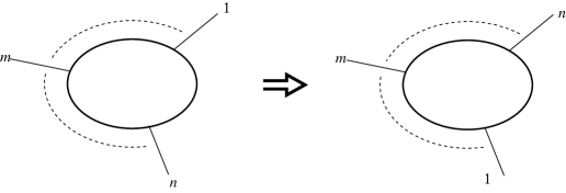
Figure 10: Flipping a tree-level amplitude.

Actually, the amplitudes $A(1,\ldots,n)$ for the bosonic string are not all independent [16]: pairs connected by world-sheet parity are in fact proportional to one another, and a closer scrutiny reveals that

$$A(1,\dots,n)=(-1)^{\sum_{i}(\alpha^{\prime}M_{i}^{2}+1)}A(n,\ldots,1)\,.$$ (38)

This crucial property may be justified noticing that $A(n,\dots,1)$ can be deformed into an amplitude with flipped external legs ordered in the sequence $(1,\ldots,n)$, as in figure 10, while on each external leg the flip $\Omega$ induces a world-sheet parity reflection, that results in a corresponding sign $(-1)^{\alpha^{\prime}M_{i}^{2}+1}$. This sign can be simply traced to the nontrivial effect of the world-sheet reflection $\sigma\to\pi-\sigma$ on the oscillator modes, that must transform as $\alpha_{k}\to(-1)^{k}\alpha_{k}$, as can be seen from eq. (22).

This “flip” symmetry has strong implications, since the four amplitudes

$$A(1,\dots,m,m+1,\ldots,n)\,,\qquad A(m,\ldots,1,m+1,\ldots,n)\,,$$

$$A(1,\ldots,m,n,\ldots,m+1)\quad{\rm and}\quad A(m,\ldots,1,n,\ldots,m+1)$$ (39)

all contribute to the same intermediate pole, and the condition (37) may be correspondingly relaxed. To be definite, let us consider the factorization of a four-vector amplitude at a vector pole in the $(1,2)$ channel. Eq. (38) suffices to show that all three-point amplitudes are proportional, being related either by cyclic symmetry or by world-sheet parity, and thus eq. (37) relaxes into the weaker condition

$${\rm tr}(\Lambda_{o}^{a_{1}}\Lambda_{o}^{a_{2}}\Lambda_{o}^{a_{3}}\Lambda_{o}^{a_{4}})-{\rm tr}(\Lambda_{o}^{a_{2}}\Lambda_{o}^{a_{1}}\Lambda_{o}^{a_{3}}\Lambda_{o}^{a_{4}})-{\rm tr}(\Lambda_{o}^{a_{1}}\Lambda_{o}^{a_{2}}\Lambda_{o}^{a_{4}}\Lambda_{o}^{a_{3}})$$

$$+{\rm tr}(\Lambda^{a_{2}}\Lambda^{a_{1}}\Lambda^{a_{4}}\Lambda^{a_{3}})={\rm tr}([\Lambda_{o}^{a_{1}},\Lambda_{o}^{a_{2}}][\Lambda_{o}^{a_{3}},\Lambda_{o}^{a_{4}}])$$

$$\sim\sum_{a_{I}}{\rm tr}([\Lambda_{o}^{a_{1}},\Lambda_{o}^{a_{2}}]\Lambda_{o}^{a_{I}}){\rm tr}(\Lambda_{o}^{a_{I}}[\Lambda_{o}^{a_{3}},\Lambda_{o}^{a_{4}}])\,,$$ (40)

where the intermediate-state matrices belong to the odd levels. The same relative signs are present for poles at all odd mass levels of the open spectrum, while even mass levels lead to the condition

$${\rm tr}(\Lambda_{o}^{a_{1}}\Lambda_{o}^{a_{2}}\Lambda_{o}^{a_{3}}\Lambda_{o}^{a_{4}})+{\rm tr}(\Lambda_{o}^{a_{2}}\Lambda_{o}^{a_{1}}\Lambda_{o}^{a_{3}}\Lambda_{o}^{a_{4}})+{\rm tr}(\Lambda_{o}^{a_{1}}\Lambda_{o}^{a_{2}}\Lambda_{o}^{a_{4}}\Lambda_{o}^{a_{3}})$$

$$+{\rm tr}(\Lambda_{o}^{a_{2}}\Lambda_{o}^{a_{1}}\Lambda_{o}^{a_{4}}\Lambda_{o}^{a_{3}})={\rm tr}(\{\Lambda_{o}^{a_{1}},\Lambda_{o}^{a_{2}}\}\{\Lambda_{o}^{a_{3}},\Lambda_{o}^{a_{4}}\})$$

$$\sim\sum_{a_{I}}{\rm tr}(\{\Lambda_{o}^{a_{1}},\Lambda_{o}^{a_{2}}\}\Lambda_{e}^{a_{I}}){\rm tr}(\Lambda_{e}^{a_{I}}\{\Lambda_{o}^{a_{3}},\Lambda_{o}^{a_{4}}\})\,,$$ (41)

where the intermediate-state matrices now belong to the even levels.

Two more cases exhaust all possibilities with four identical external states: four even states into one odd or into one even state. Summarizing, we have thus obtained the four conditions

$$({\rm four\ odd}\to{\rm odd}):$$

$${\rm tr}([\Lambda_{o}^{a_{1}},\Lambda_{o}^{a_{2}}][\Lambda_{o}^{a_{3}},\Lambda_{o}^{a_{4}}])\sim\sum_{a_{I}}{\rm tr}([\Lambda_{o}^{a_{1}},\Lambda_{o}^{a_{2}}]\Lambda_{o}^{a_{I}}){\rm tr}(\Lambda_{o}^{a_{I}}[\Lambda_{o}^{a_{3}},\Lambda_{o}^{a_{4}}])\,,$$

$$({\rm four\ odd}\to{\rm even}):$$

$${\rm tr}(\{\Lambda_{o}^{a_{1}},\Lambda_{o}^{a_{2}}\}\{\Lambda_{o}^{a_{3}},\Lambda_{o}^{a_{4}}\})\sim\sum_{a_{I}}{\rm tr}(\{\Lambda_{o}^{a_{1}},\Lambda_{o}^{a_{2}}\}\Lambda_{e}^{a_{I}}){\rm tr}(\Lambda_{e}^{a_{I}}\{\Lambda_{o}^{a_{3}},\Lambda_{o}^{a_{4}}\})\,,$$

$$({\rm four\ even}\to{\rm odd}):$$

$${\rm tr}([\Lambda_{e}^{a_{1}},\Lambda_{e}^{a_{2}}][\Lambda_{e}^{a_{3}},\Lambda_{e}^{a_{4}}])\sim\sum_{a_{I}}{\rm tr}([\Lambda_{e}^{a_{1}},\Lambda_{e}^{a_{2}}]\Lambda_{o}^{a_{I}}){\rm tr}(\Lambda_{o}^{a_{I}}[\Lambda_{e}^{a_{3}},\Lambda_{e}^{a_{4}}])\,,$$

$$({\rm four\ even}\to{\rm even}):$$ (42)

$${\rm tr}(\{\Lambda_{e}^{a_{1}},\Lambda_{e}^{a_{2}}\}\{\Lambda_{e}^{a_{3}},\Lambda_{e}^{a_{4}}\})\sim\sum_{a_{I}}{\rm tr}(\{\Lambda_{e}^{a_{1}},\Lambda_{e}^{a_{2}}\}\Lambda_{e}^{a_{I}}){\rm tr}(\Lambda_{e}^{a_{I}}\{\Lambda_{e}^{a_{3}},\Lambda_{e}^{a_{4}}\})\,,$$

where the labels $e$ and $o$ anticipate the freedom of associating different Chan-Paton matrices to the even and odd mass levels of the open spectrum, and these imply generalized completeness conditions of the type

$$[\Lambda_{o},\Lambda_{o}]\sim i\,\Lambda_{o}\,,\quad[\Lambda_{e},\Lambda_{e}]\sim i\,\Lambda_{o}\,,\quad[\Lambda_{e},\Lambda_{o}]\sim i\,\Lambda_{e}\,,$$

$$\{\Lambda_{o},\Lambda_{o}\}\sim\Lambda_{e}\,,\quad\{\Lambda_{e},\Lambda_{e}\}\sim\Lambda_{e}\,,\quad\{\Lambda_{e},\Lambda_{o}\}\sim\Lambda_{o}\,.$$ (43)

Once the dynamical parts of the amplitudes are given a proper normalization, consistently with the flip condition (38), one ought to supplement eqs. (43) with additional hermiticity conditions, necessary to guarantee the proper sign of physical residues. For definiteness, let us imagine to have normalized all two-point functions so that the $\Lambda$’s are all hermitian. The algebraic content of eqs. (43) is then easier to appreciate in terms of the two auxiliary sets

$$\lambda=\{\Lambda_{e}\}\,,\qquad\mu=\{i\Lambda_{o}\}\,,$$ (44)

since, on account of (43), the $\lambda$’s and $\mu$’s may be regarded as basis elements of a real associative algebra, a vector space closed under multiplication. One is thus led to classify the irreducible real associative algebras. As in the case of Lie algebras, the problem simplifies if one considers the complex extension since, on account of Wedderburn’s theorem [101], the only irreducible solutions are then the full matrix algebras ${\rm GL}(n,\hbox{\mbm C})$.

Our next task is to recover the original non-complexified form of the algebra generated by the two sets $\lambda$ and $\mu$, and to this end we should distinguish two cases. If the original algebra contains an element that squares to $-1$, it coincides with its complex extension, and is itself ${\rm GL}(n,\hbox{\mbm C})$. In this case the $\mu$’s are antihermitian generators of ${\rm U}(n)$, while the $\lambda$’s are the remaining hermitian generators of ${\rm GL}(n,\hbox{\mbm C})$. States of even and odd mass levels are now defined by equivalent $\Lambda_{e}$ and $\Lambda_{o}$ matrices, and are thus all valued in the adjoint representation of ${\rm U}(n)$. On the other hand, if the original algebra does not contain an element that squares to $-1$, on account of the first line of eq. (43), it is a real form of ${\rm GL}(n,\hbox{\mbm C})$ that, besides being an algebra, is also a Lie algebra. A corollary of Wedderburn’s theorem states that these real forms are only ${\rm GL}(n,\hbox{\mbm R})$ and, in the even, $2n$, case, ${\rm GL}(n,\hbox{\mbm Q})$. ${\rm GL}(n,\hbox{\mbm R})$ defines antisymmetric $\Lambda_{o}$ matrices that span the adjoint representation of ${\rm SO}(n)$ and symmetric $\Lambda_{e}$ matrices corresponding to the symmetric traceless and singlet representations of ${\rm SO}(n)$. Finally, ${\rm GL}(n,\hbox{\mbm Q})$ defines $\Lambda_{o}$ matrices that span the adjoint representation of ${\rm USp}(2n)$ and $\Lambda_{e}$ matrices corresponding to the traceless antisymmetric and singlet representations of ${\rm USp}(2n)$. The factorization of higher-point functions leads to additional sets of conditions, that we shall refrain from writing explicitly. All, however, are satisfied by these solutions, as can be seen by direct substitution. One can summarize these results saying that the ends of an open string are valued in the (anti)fundamental representations of one of the classical groups ${\rm U}(n)$, ${\rm SO}(n)$ and ${\rm USp}(2n)$.

It is interesting to recover these gauge groups and the corresponding representations from the dynamics of additional degrees of freedom living at the two ends of an open string [33]. This can be done adding an even number $n$ of one-dimensional fermions $\psi_{I}$, with a corresponding action

$$S={\textstyle\frac{1}{4}}\ \int_{\partial\Sigma}\ ds\ i\ \eta^{IJ}\ \psi_{I}\frac{d\psi_{J}}{ds}\,,$$ (45)

where $\partial\Sigma$ denotes the world-sheet boundary and, for the time being, $\eta$ is a Minkowski-like metric with $t$ time-like and $s$ space-like directions. Canonical quantization then results in the Clifford algebra

$$\{\psi_{I},\psi_{J}\}=2\eta_{IJ}\,,$$ (46)

and the two ends of an open string are thus to fill the corresponding representation, of dimension $2^{n/2}$, so that each is now endowed with as many “colours”.

A related result may be obtained from the contribution of a single empty closed boundary, along which the fermions of eq. (45) are naturally antiperiodic. For a pair of $\psi$ fields the finite contribution to the resulting determinant, free of zero modes, is independent of the length $l$ of the boundary. It may be conveniently calculated from the corresponding antiperiodic $\zeta$ function, as

$${\rm det}\left(-{\textstyle\frac{1}{4}}\ \frac{\partial^{2}}{\partial s^{2}}\right) = \lim_{p\to 0}\ \exp\left\{-\frac{d}{dp}\left[\left(\frac{\pi}{2l}\right)^{-2p}\ (2^{-2p}-1)\zeta(2p)\right]\right\}$$ (47)

$$= \exp[-2\zeta(0)\log 2]\,,$$

where $\zeta$ denotes the Riemann $\zeta$ function and $\zeta(0)=-\frac{1}{2}$, and the end result is therefore $2$, consistently with the Clifford algebra (46).

In a similar fashion, one can associate internal quantum numbers to open-string states via corresponding dressings of their vertex operators. These are to be regarded as bi-spinors $V_{\alpha\beta}$, and involve corresponding expansions in terms of the $\psi^{I}$ fields:

$$V_{\alpha\beta}=\delta_{\alpha\beta}+{(\gamma^{I})}_{\alpha\beta}\psi_{I}+\ldots+{(\gamma^{I_{1}\ldots I_{p}})}_{\alpha\beta}\psi_{I_{1}}\ldots\psi_{I_{p}}+\ldots\,.$$ (48)

The correlation functions of these vertex operators now include contributions from the fermions $\psi_{I}$, whose Green function is a simple square wave for any closed boundary and, as a result, one can see that the Chan-Paton factors of eq. (35) can be recovered from correlators of $\psi$ fields. This setting has been widely used in [102] to derive low-energy open-string couplings, in the spirit of the $\sigma$-model constructions in [103].

Taking these fermion fields more seriously, one can actually go a bit further. To this end, let us anticipate a result to be discussed in detail in later sections: for the bosonic string, there is a special gauge group, SO(8192), that from our previous considerations can be built with 26 boundary fermions. Let us recall that, as we have seen, each end of the open string is valued in the spinor representation of the manifest symmetry group of the action (45). For unoriented strings, whose states are eigenstates of the “flip” operator $\Omega$, the bi-spinor field $V$ of eq. (48) satisfies a corresponding reality condition. This can be consistently imposed both in the real, $s-t=0,2\ {\rm mod\ }8$, and pseudo-real, $s-t=4,6\ {\rm mod\ }8$, cases, since it is imposed simultaneously on both indices of $V_{\alpha\beta}$. However, the resulting Chan-Paton group is ${\rm SO}(2^{n/2})$ in the first case and ${\rm USp}(2^{n/2})$ in the second. Thus, it is SO(8192) precisely with $26$ boundary fermions, as many as the string coordinates, and with the same signature. A related, amusing observation, is that only in this case the linear divergence, proportional to the length of the boundary, present in the determinant of the Laplace operator for the string coordinates, naturally compensates a similar divergence of the fermion determinant, that we have not seen explicitly having used the $\zeta$-function method. Although this simple setting can naturally recover classical groups whose order is a power of two, it is apparently less natural to adapt it to cases where the gauge groups have a reduced rank.

2.4 Vacuum amplitudes with zero Euler character

In Field Theory, one usually does not pay much attention to the one-loop vacuum amplitude. This is a function of the masses of the finite number of fields of a given model, fully determined by the free spectrum [106] that, aside from its relation to the cosmological constant, does not embody important structural information. On the other hand, strings describe infinitely many modes, and their vacuum amplitudes satisfy a number of geometric constraints, that in a wide class of models essentially determine the full perturbative spectrum.

In order to define the vacuum amplitudes for closed and open strings, it is convenient to start from Field Theory, and in particular from the simplest case of a scalar mode of mass $M$ in $D$ dimensions, for which

$$S=\int\ d^{D}x\left({\textstyle\frac{1}{2}}\,\partial_{\mu}\phi\ \partial^{\mu}\phi-{\textstyle\frac{1}{2}}\,M^{2}\phi^{2}\right)\,.$$ (49)

After a Euclidean rotation, the path integral defines the vacuum energy $\Gamma$ as

$$e^{-\Gamma}=\int[D\phi]e^{-S_{E}}\sim{\rm det}^{-\frac{1}{2}}\left(-\Delta+M^{2}\right)\,,$$ (50)

whose $M$ dependence may be extracted using the identity

$$\log\left({\rm det}(A)\right)=-\int_{\epsilon}^{\infty}\ \frac{dt}{t}\ {\rm tr}\left(e^{-tA}\right)\,,$$ (51)

where $\epsilon$ is an ultraviolet cutoff and $t$ is a Schwinger parameter. In our case, the complete set of momentum eigenstates diagonalizes the kinetic operator, and

$$\Gamma=-\frac{V}{2}\ \int_{\epsilon}^{\infty}\ \frac{dt}{t}\ e^{-tM^{2}}\ \int\ \frac{d^{D}p}{(2\pi)^{D}}\ e^{-tp^{2}}\,,$$ (52)

where $V$ denotes the volume of space-time. Performing the Gaussian momentum integral then yields

$$\Gamma=-\frac{V}{2(4\pi)^{D/2}}\ \int_{\epsilon}^{\infty}\ \frac{dt}{t^{D/2+1}}\ e^{-tM^{2}}\,,$$ (53)

while similar steps for a Dirac fermion of mass $M$ in $D$ dimensions would result in

$$\Gamma=\frac{V2^{[D/2]}}{2(4\pi)^{D/2}}\ \int_{\epsilon}^{\infty}\ \frac{dt}{t^{D/2+1}}\ e^{-tM^{2}}\,,$$ (54)

with an opposite sign, on account of the Grassmann nature of the fermionic path integral. These results can be easily extended to generic Bose or Fermi fields, since $\Gamma$ is only sensitive to their physical modes, and is proportional to their number. Therefore, in the general case they are neatly summarized in the expression

$$\Gamma_{\rm tot}=-\frac{V}{2(4\pi)^{D/2}}\ \int_{\epsilon}^{\infty}\ \frac{dt}{t^{D/2+1}}\ {\rm Str}\left(e^{-tM^{2}}\right)\,,$$ (55)

where ${\rm Str}$ counts the signed multiplicities of Bose and Fermi states.

We can now try to apply eq. (55) to the closed bosonic string in the critical dimension $D=26$, whose spectrum, described at the end of subsection 2.2, is encoded in

$$M^{2}=\frac{2}{\alpha^{\prime}}\left(L_{0}+\bar{L}_{0}-2\right)\,,$$ (56)

subject to the constraint $L_{0}=\bar{L}_{0}$. Substituting (56) in (55) then gives

$$\Gamma_{\rm tot}=-\frac{V}{2(4\pi)^{13}}\int_{\epsilon}^{\infty}\frac{dt}{t^{14}}\ {\rm tr}\ \left(e^{-\frac{2}{\alpha^{\prime}}(L_{0}+\bar{L}_{0}-2)t}\right)\,,$$ (57)

an expression that is not quite correct, since it does not take into account the “level-matching” condition $L_{0}=\bar{L}_{0}$ for the physical states that, however, can be simply accounted for introducing a $\delta$-function constraint in (57), so that

$$\Gamma_{\rm tot}=-\frac{V}{2(4\pi)^{13}}\int_{-\,\frac{1}{2}}^{\frac{1}{2}}ds\int_{\epsilon}^{\infty}\frac{dt}{t^{14}}\ {\rm tr}\left(\ e^{-\frac{2}{\alpha^{\prime}}(L_{0}+\bar{L}_{0}-2)t}e^{2\pi i(L_{0}-\bar{L}_{0})s}\right)\,,$$ (58)

since, from our previous discussion, $L_{0}-\bar{L}_{0}$ has integer eigenvalues. Defining the “complex” Schwinger parameter

$$\tau=\tau_{1}+i\tau_{2}=s+i\frac{t}{\alpha^{\prime}\pi}\,,$$ (59)

and letting

$$q=e^{2\pi i\tau}\,,\qquad\bar{q}=e^{-2\pi i\bar{\tau}}\,,$$ (60)

eq. (58) takes the more elegant form

$$\Gamma_{\rm tot}=-\frac{V}{2(4\pi^{2}\alpha^{\prime})^{13}}\ \int_{-\,\frac{1}{2}}^{\frac{1}{2}}d\tau_{1}\ \int_{\epsilon}^{\infty}\ \frac{d\tau_{2}}{\tau_{2}^{14}}\ {\rm tr}\ q^{L_{0}-1}\bar{q}^{\bar{L}_{0}-1}\,.$$ (61)

Actually, at one loop a closed string sweeps a torus, whose Teichmüller parameter is naturally identified with the complex Schwinger parameter $\tau$ but, as we have seen in subsection 2.1, not all values of $\tau$ within the strip $\{-\,\frac{1}{2}<\tau_{1}\leq\frac{1}{2},\epsilon<\tau_{2}<\infty\}$ of eq. (61) correspond to distinct tori. Hence, one should restrict the integration domain to a fundamental region of the modular group, for instance to the region ${\cal F}$ of eq. (7), and the restriction to ${\cal F}$ introduces an effective ultraviolet cutoff, of the order of the string scale, for all string modes. After a final rescaling, we are thus led to an important quantity, the torus amplitude, that defines the partition function for the closed bosonic string

$${\cal T}=\int_{\cal F}\ \frac{d^{2}\tau}{\tau_{2}^{2}}\ \frac{1}{\tau_{2}^{12}}\ {\rm tr}\ q^{L_{0}-1}\bar{q}^{\bar{L}_{0}-1}\,.$$ (62)

This type of expression actually determines the vacuum amplitude for any model of oriented closed strings, once the corresponding Virasoro operators $L_{0}$ and $\bar{L}_{0}$ are known.

It is instructive to compute explicitly the torus amplitude (62) for the bosonic string. To this end, we should recall that $L_{0}$ and $\bar{L}_{0}$ are effectively number operators for two infinite sets of harmonic oscillators. In particular, in terms of conventionally normalized creation and annihilation operators, for each transverse space-time dimension

$$L_{0}=\sum_{n}\ n\ a^{\dagger}_{n}\ a_{n}\,,$$ (63)

while for each $n$

$${\rm tr}\ q^{n\,a^{\dagger}_{n}a_{n}}=1+q^{n}+q^{2n}+\ldots=\frac{1}{1-q^{n}}\,,$$ (64)

and putting all these contributions together for the full spectrum gives

$${\cal T}=\int_{\cal F}\ \frac{d^{2}\tau}{\tau_{2}^{2}}\ \frac{1}{\tau_{2}^{12}}\ \frac{1}{|\eta(\tau)|^{48}}\,,$$ (65)

where we have defined the Dedekind $\eta$ function

$$\eta(\tau)=q^{\frac{1}{24}}\,\prod_{n=1}^{\infty}\ (1-q^{n})\,.$$ (66)

The integrand of ${\cal T}$ is indeed invariant under the modular group, as originally noticed by Shapiro [24], since the measure is invariant under the two generators $S$ and $T$ while, using the transformations [107]

$$T:\ \eta(\tau+1)=e^{\frac{i\pi}{12}}\,\eta(\tau)\,,\qquad S:\ \eta(-1/\tau)=\sqrt{-i\tau}\ \eta(\tau)\,,$$ (67)

one can verify that the combination $\tau_{2}^{1/2}|\eta|^{2}$ is also invariant. In other words, modular invariance holds separately for the contribution of each transverse string coordinate, independently of their total number, i.e. independently of the total central charge $c$. This is a crucial property of the conformal field theories that define the torus amplitudes for all consistent models of oriented closed strings.

In the case at hand all string states are oscillator excitations of the tachyonic vacuum, while the factor $\tau_{2}^{-12}$ can be recovered from the integral over the continuum of transverse momentum modes, as

$$(\alpha^{\prime})^{12}\ \int\ d^{24}p\ e^{-\pi\alpha^{\prime}\tau_{2}p^{2}}\,,$$ (68)

so that the partition function (65) can be written in the form

$${\cal T}=(\alpha^{\prime})^{12}\ \int_{\cal F}\ \frac{d^{2}\tau}{\tau_{2}^{2}}\ \int\ d^{24}p\ \left|\frac{q^{\frac{\alpha^{\prime}}{4}p^{2}}}{\eta(\tau)^{24}}\right|^{2}\,,$$ (69)

that exhibits a continuum of distinct ground states with corresponding towers of excitations. In the language of Conformal Field Theory, each tower is a “Verma module” [21, 23], while the squared masses of the ground states are determined by the conformal weights $h_{i}$ of the primaries. The content of each Verma module may be encoded in a corresponding character

$$\chi_{i}(q)={\rm tr}\left(q^{L_{0}-c/24}\right)_{i}=q^{h_{i}-c/24}\sum_{k}d_{k}q^{k}\,,$$ (70)

where the $d_{k}$ are positive integers that count the multiplicities of the corresponding excitations, of weights $(h_{i}+k)$. In terms of these characters, a general torus amplitude would read

$${\cal T}=\int_{\cal F}\ \frac{d^{2}\tau}{\tau_{2}^{2}}\ \sum_{i,j}\bar{\chi}_{i}(\bar{q})\ X_{ij}\ \chi_{j}(q)\,,$$ (71)

with $X$ an integer matrix that counts their signed multiplicities, as determined by spin-statistics. The 26-dimensional bosonic string thus belongs to this type of setting, with the double sum over Verma modules replaced by an integral over the continuum of its transverse momentum modes, each associated to a Virasoro character

$$\chi_{p}(q)=\frac{q^{\frac{\alpha^{\prime}}{4}p^{2}}}{\eta(\tau)^{24}}\,.$$ (72)

We are now ready to meet the first and simplest instance of an orientifold or open descendant [36], where world-sheet parity is used to project a closed spectrum. Let us begin by recalling the low-lying spectrum of the closed bosonic string that, as we have seen, starts with a tachyonic scalar, followed by the massless modes associated to $\alpha_{-1}^{i}\tilde{\alpha}_{-1}^{j}|0\tilde{0}\rangle$: a traceless symmetric tensor, a scalar mode, identified with the trace, and an antisymmetric tensor. We would like to stress that these states and all the higher excitations have a definite symmetry under the interchange of left, $\alpha$, and right, $\tilde{\alpha}$, oscillator modes. Indeed, both the action and the quantization procedure used preserve the world-sheet parity $\Omega$, while this operation squares to the identity, and thus splits the whole string spectrum in two subsets of states, corresponding to its two eigenvalues, $\pm 1$. Naïvely, one could conceive to project the spectrum retaining either of these two subsets, but string states can scatter, and the product of two odd states would generate even ones. Hence, in this case one has the unique option of retaining only the states invariant under world-sheet parity, and this eliminates, in particular, the massless antisymmetric two-tensor. Therefore, after the projection the massless level, that in the original model contained $(24)^{2}$ states, contains only $24\,(24+1)/2$ states.

In order to account for the multiplicities in the projected spectrum, one is thus to halve the torus contribution and to supplement it with an additional term, where left and right modes are effectively identified. This is accomplished by the Klein-bottle amplitude, that describes a vacuum diagram drawn by a closed string undergoing a reversal of its orientation. From an operatorial viewpoint, one is computing a trace over the string states with an insertion of the world-sheet parity operator $\Omega$:

$${\cal K}={\textstyle\frac{1}{2}}\ \int_{{\cal F}_{\cal K}}\ \frac{d^{2}\tau}{\tau_{2}^{2}}\ \frac{1}{\tau_{2}^{12}}{\rm tr}\left(q^{L_{0}-1}\ \bar{q}^{\bar{L}_{0}-1}\ \Omega\right)\,.$$ (73)

More explicitly, the inner trace can be written

$$\sum_{{\rm L},{\rm R}}\langle{\rm L},{\rm R}|\ q^{L_{0}-1}\ \bar{q}^{\bar{L}_{0}-1}\ \Omega\ |{\rm L},{\rm R}\rangle$$ (74)

and, after using $\Omega|{\rm L},{\rm R}\rangle=|{\rm R},{\rm L}\rangle$, that, as we have anticipated, is the only available choice in this case, and the orthonormality conditions for the states, reduces to

$$\sum_{{\rm L},{\rm R}}\langle{\rm L},{\rm R}|\ q^{L_{0}-1}\ \bar{q}^{\bar{L}_{0}-1}\ |{\rm R},{\rm L}\rangle=\sum_{\rm L}\langle{\rm L},{\rm L}|\ (q\bar{q})^{L_{0}-1}\ |{\rm L},{\rm L}\rangle\,,$$ (75)

where the restriction to the diagonal subset $|{\rm L},{\rm L}\rangle$ has led to the effective identification of $L_{0}$ and $\bar{L}_{0}$.

It should be appreciated that the resulting amplitude depends naturally on $2i\tau_{2}$ that, as we have seen, is the modulus of the doubly-covering torus. The integration domain, not fully determined by these considerations, is necessarily the whole positive imaginary axis of the $\tau$ plane, since the involution breaks the modular group to a finite subgroup. In conclusion, after performing the trace, for the bosonic string one finds

$${\cal K}={\textstyle\frac{1}{2}}\ \int_{0}^{\infty}\ \frac{d\tau_{2}}{\tau_{2}^{14}}\ \frac{1}{\eta^{24}(2i\tau_{2})}\,.$$ (76)

It is instructive to compare the $q$ expansions of the integrands of ${\cal T}$ and ${\cal K}$, while retaining in the former only terms with equal powers of $q$ and $\bar{q}$, that correspond to on-shell physical states satisfying the level-matching condition. Aside from powers of $\tau_{2}$, these integrands are

$${\cal T} \rightarrow \left((q\bar{q})^{-1}+(24)^{2}+\ldots\right)\,,$$

$${\cal K} \rightarrow {\textstyle\frac{1}{2}}\left((q\bar{q})^{-1}+(24)+\ldots\right)\,,$$ (77)

and therefore the right counting of states in the projected spectrum is indeed attained halving the torus amplitude ${\cal T}$ and adding to it the Klein-bottle amplitude ${\cal K}$.

Following [30, 33], let us now use as integration variable the modulus $t=2\tau_{2}$ of the double cover of the Klein bottle. The corresponding transformation recovers a very important power of two, that we have already met in the discussion of the “quarks” at the ends of the open string, and indeed, taking into account the rescaling of the integration measure gives

$${\cal K}=\frac{2^{13}}{2}\ \int_{0}^{\infty}\ \frac{dt}{t^{14}}\ \frac{1}{\eta^{24}(it)}\,.$$ (78)

In our description of the Klein bottle in subsection 2.1, we have emphasized that this surface allows for two distinct natural choices of “time”. The vertical time, $\tau_{2}$, enters the operatorial definition of the trace, and defines the direct-channel or loop amplitude, while the horizontal time, $\ell=1/t$, displays the Klein bottle as a tube terminating at two crosscaps, and defines the transverse-channel or tree amplitude. The corresponding expression, that we denote by $\tilde{\cal K}$,

$$\tilde{\cal K}=\frac{2^{13}}{2}\ \int_{0}^{\infty}\ d\ell\ \frac{1}{\eta^{24}(i\ell)}$$ (79)

can be obtained from eq. (78) by an $S$ modular transformation.

Let us now turn to the annulus amplitude. In this case, the trace is over the open spectrum and, in order to account for the internal Chan-Paton symmetry, we associate a multiplicity $N$ to each of the string ends. As in the previous case, let us begin from the direct-channel amplitude, defined in terms of a trace over open-string states,

$${\cal A}=\frac{N^{2}}{2}\ \int_{0}^{\infty}\ \frac{d\tau_{2}}{\tau_{2}^{14}}\ {\rm tr}(q^{\frac{1}{2}(L_{0}-1)})\,,$$ (80)

where the exponent is now rescaled as demanded by the different Regge slope of the open spectrum, exhibited in eq. (34). Computing the trace as above one finds

$${\cal A}=\frac{N^{2}}{2}\ \int_{0}^{\infty}\ \frac{d\tau_{2}}{\tau_{2}^{14}}\ \frac{1}{\eta^{24}\left(\frac{1}{2}i\tau_{2}\right)}\,,$$ (81)

and once more the amplitude is naturally expressed in terms of the modulus, now ${1\over 2}i\tau_{2}$, of the doubly-covering torus. The first terms in the expansion of the integrand in powers of $\sqrt{q}$ give

$${\cal A}\rightarrow\frac{N^{2}}{2}\left((\sqrt{q})^{-1}+(24)+\ldots\right)$$ (82)

and, as for the Klein bottle, it is convenient to move to the modulus of the double cover, now $t=\tau_{2}/2$, as integration variable, obtaining

$${\cal A}=\frac{N^{2}\ 2^{-13}}{2}\ \int_{0}^{\infty}\ \frac{dt}{t^{14}}\ \frac{1}{\eta^{24}(it)}\,.$$ (83)

The other choice of time, $\ell=1/t$, then displays the annulus as a tube terminating at two holes, and defines the transverse-channel amplitude. The corresponding expression, that we denote by $\tilde{\cal A}$,

$$\tilde{\cal A}=\frac{N^{2}\ 2^{-13}}{2}\ \int_{0}^{\infty}\ d\ell\ \frac{1}{\eta^{24}(i\ell)}\,,$$ (84)

can be obtained from eq. (83) by an $S$ modular transformation. It should be appreciated that, in this tree channel, the multiplicity $N$ of the Chan-Paton charge spaces associated to the ends of the open string determines the reflection coefficients for the closed spectrum in front of the two boundaries.

The Möbius strip presents some additional subtleties. This can be anticipated, since the discussion of the other two amplitudes suggests that the corresponding integrand should depend on the modulus of the doubly-covering torus. In this case, however, as we have seen in subsection 2.1, this is not purely imaginary but has a fixed real part, equal to $\frac{1}{2}$, that introduces relative signs for the oscillator excitations at the various mass levels. These are precisely the signs discussed in the previous subsection, as can be appreciated from the limiting behaviour of the amplitude for large vertical time, that exhibits the contributions of intermediate open-string states undergoing a flip of their orientation.

While the integrand is obviously real for both ${\cal K}$ and ${\cal A}$, that depend on an imaginary modulus, the same is not true for the Möbius amplitude ${\cal M}$, where $\tau_{1}=\frac{1}{2}$. In order to write it for generic models, that can include several Verma modules with primaries of different weights, it is convenient to introduce a basis of real “hatted” characters, defined as

$$\hat{\chi}_{i}(i\tau_{2}+{\textstyle{1\over 2}})=q^{h_{i}-c/24}\sum_{k}(-1)^{k}d_{(i)k}q^{k}\,,$$ (85)

where $q=e^{-2\pi\tau_{2}}$, that differ from $\chi_{i}(i\tau_{2}+\frac{1}{2})$ in the overall phases $e^{-i\pi(h_{i}-c/24)}$. This redefinition affects the modular transformation $P$ connecting direct and transverse Möbius amplitudes, ${\cal M}$ and $\tilde{\cal M}$, that now becomes

$$P=T^{1/2}\ S\ T^{2}\ S\ T^{1/2}\,,$$ (86)

where $T^{1/2}$ is a diagonal matrix, with $T^{1/2}_{ij}=\delta_{ij}\,e^{i\pi(h_{i}-c/24)}$. For a generic conformal field theory, using the constraints

$$S^{2}=(ST)^{3}={\cal C}\,,$$ (87)

it is simple to show that

$$P^{2}={\cal C}\,,$$ (88)

so that $P$ shares with $S$ the important property of squaring to the conjugation matrix ${\cal C}$. In the last section we shall elaborate on the rôle of $P$, and of this property in particular, in Boundary Conformal Field Theory.

Returning to the open bosonic string, the Möbius amplitude finally takes the form

$${\cal M}=\frac{\epsilon\,N}{2}\int_{0}^{\infty}\ \frac{d\tau_{2}}{\tau_{2}^{14}}\ \frac{1}{\hat{\eta}^{24}({\textstyle{1\over 2}}i\tau_{2}+{\textstyle{1\over 2}})}\,,$$ (89)

where $\epsilon$, equal to $\pm 1$, is an overall sign, and its expansion in powers of $\sqrt{q}$ gives

$${\cal M}\rightarrow\frac{\epsilon\,N}{2}\left((\sqrt{q})^{-1}-(24)+\ldots\right)\,.$$ (90)

Then, from eqs. (82) and (90), $\epsilon=+1$ corresponds to a total of $N(N-1)/2$ massless vectors, and thus to an orthogonal gauge group, while (for even $N$) $\epsilon=-1$ corresponds to a symplectic gauge group.

In this case the transition to the transverse channel requires, as we have emphasized, the redefinition $\tau_{2}\to 1/t$ and the corresponding $P$ transformation. It is then simple to show that

$$\hat{\eta}\left(\frac{i}{2t}+\frac{1}{2}\right)=\sqrt{t}\ \hat{\eta}\left(\frac{it}{2}+\frac{1}{2}\right)\,,$$ (91)

and therefore

$$\tilde{\cal M}=\frac{\epsilon\,N}{2}\int_{0}^{\infty}\ dt\ \frac{1}{\hat{\eta}^{24}({\textstyle{1\over 2}}it+{\textstyle{1\over 2}})}$$ (92)

or, in terms of $\ell=t/2$,

$$\tilde{\cal M}=2\ \frac{\epsilon\,N}{2}\int_{0}^{\infty}\ d\ell\ \frac{1}{\hat{\eta}^{24}(i\ell+{\textstyle{1\over 2}})}\,.$$ (93)

The additional factor of two introduced by the last redefinition is very important, since it reflects the combinatorics of the vacuum channel: as we have seen, $\tilde{\cal M}$ may be associated to a tube with one hole and one crosscap at the ends, and thus needs precisely a combinatoric factor of two compared to $\tilde{\cal K}$ and $\tilde{\cal A}$, while the sign $\epsilon$ is a relative phase between crosscap and boundary reflection coefficients. Finally, the Chan-Paton multiplicity $N$ determines the reflection coefficient for the closed string in front of the single boundary present in the tree channel.

Figure 11: Tadpole conditions in orientifold models.

One can now study the limiting ultraviolet behaviour of the four amplitudes of vanishing Euler character for small vertical time. As we have seen, the torus ${\cal T}$ is formally protected by modular invariance, that excludes the ultraviolet region from the integration domain. On the other hand, for the other three surfaces the integration regions touch the real axis, and introduce corresponding ultraviolet divergences. In order to take a closer look, it is convenient to turn to the transverse channel, where the divergences appear in the infrared, or large $\ell$, limit of eqs. (79), (84) and (93), and clearly originate from the exchange of tachyonic and massless modes. In general, a state of mass $M$ gives a contribution proportional to

$$\int_{0}^{\infty}\ d\ell\ e^{-M^{2}\ \ell}=\frac{1}{M^{2}}\,,$$ (94)

and therefore, although one can formally regulate the tachyonic divergence, there is no way to regulate the massless exchanges. It should be appreciated that all massive states give sizable contributions only for $\ell\leq 1/M^{2}$. Thus, once the massless term is eliminated, the vertical time ultraviolet region inherits a natural cutoff of the order of the string scale, precisely as was the case for oriented closed strings on account of modular invariance. In this simple model, Lorentz invariance clearly associates the singular exchange to the only massless scalar mode of the closed string, the dilaton. Moreover, it is simple to convince oneself that, as suggested by eq. (94), the divergence has a simple origin, clearly exhibited in the factorization limit $\ell\to\infty$: the propagator $1/(p^{2}+M^{2})$ diverges for a massless state of zero momentum. This is a very important point, since the corresponding residues are actually finite, and define two basic building blocks of the theory, the one-point functions for closed-string fields in front of a boundary and in front of a crosscap. Since the former is proportional to the dimension $N$ of the Chan-Paton charge space, the two contributions can cancel one another, leading to a finite amplitude, only for a single choice of Chan-Paton gauge group. More in detail, the singular terms of eqs. (79), (84) and (93) group into a contribution proportional to

$$\tilde{\cal K}+\tilde{\cal A}+\tilde{\cal M}\sim{\textstyle\frac{1}{2}}\ (2^{13}+2^{-13}\ N^{2}-2\,\epsilon\,N)=\frac{2^{-13}}{2}\ (N-\epsilon\,2^{13})^{2}\,,$$ (95)

that clearly vanishes for $N=2^{13}=8192$ and $\epsilon=+1$, and thus for the Chan-Paton gauge group SO(8192) [31, 32, 33, 34]. This is our first encounter with a tadpole condition.

While in this model the special choice of $N$ eliminates a well-defined correction to the low-energy effective field theory, a potential for the dilaton $\varphi$

$$V\sim(N-\epsilon\,2^{13})\,\int\,d^{26}x\ \sqrt{-g}\ e^{-\varphi}\,,$$ (96)

with $g$ the space-time metric, whose functional form is fully determined by general covariance and by the Euler characters of disk and crosscap, in more complicated cases, as we shall soon see, one can similarly dispose of some inconsistent contributions, thus eliminating corresponding anomalies in gauge and gravitational currents [35]. In this sense, tadpole cancellations provide the very rationale for the appearance of the open sector.

Let us recall the steps that have led to the SO(8192) model of unoriented open and closed strings. The direct-channel Klein bottle amplitude ${\cal K}$ receives contributions only from states of the oriented closed spectrum built symmetrically out of left and right oscillator modes, and completes the projection of the closed spectrum to states symmetric under world-sheet parity. The corresponding transverse channel amplitude $\tilde{\cal K}$ receives contributions only from states that can be reflected compatibly with 26-dimensional Lorentz invariance. It may be obtained rescaling the integration variable to the modulus of the doubly-covering torus and performing an $S$ modular transformation, describes the propagation of the projected closed spectrum on a tube terminating at two crosscaps, and is thus quadratic in the corresponding reflection coefficients. In a similar fashion, the transverse-channel annulus amplitude $\tilde{\cal A}$ describes the propagation of the projected closed spectrum on a tube terminating at two boundaries compatibly with 26-dimensional Lorentz invariance, and is thus quadratic in the corresponding reflection coefficients, that are proportional to the overall Chan-Paton multiplicity $N$. The corresponding direct-channel amplitude ${\cal A}$, the one-loop vacuum amplitude for the open string, may be recovered by a rescaling of the integration variable and an $S^{-1}$ transformation. In this picture, $N$ describes the Chan-Paton multiplicity associated to an end of the open string. Finally, the transverse-channel Möbius amplitude $\tilde{\cal M}$ describes the propagation of the projected closed spectrum on a tube terminating at one hole and one crosscap, and as such is a “geometric mean” of $\tilde{\cal K}$ and $\tilde{\cal A}$, an operation that leaves a sign $\epsilon$ undetermined. A rescaling of the integration variable and a $P^{-1}$ transformation turn it into the direct-channel amplitude ${\cal M}$, that completes the projection of the open spectrum.

In conclusion, leaving the integrations implicit, the open descendants of the 26-dimensional bosonic string are described by

$${\textstyle\frac{1}{2}}{\cal T} = {\textstyle\frac{1}{2}}\ \frac{1}{\tau_{2}^{12}\ |\eta(\tau)|^{48}}\,,$$

$${\cal K} = {\textstyle\frac{1}{2}}\ \frac{1}{\tau_{2}^{12}\ \eta(2i\tau_{2})^{24}}\,,$$ (97)

that define the projected unoriented closed spectrum, and by

$${\cal A} = \frac{N^{2}}{2}\ \frac{1}{\tau_{2}^{12}\ \eta({\textstyle{1\over 2}}i\tau_{2})^{24}}\,,$$

$${\cal M} = \frac{\epsilon\,N}{2}\ \frac{1}{\tau_{2}^{12}\ \hat{\eta}({\textstyle{1\over 2}}i\tau_{2}+{\textstyle{1\over 2}})^{24}}\,,$$ (98)

that define the projected unoriented open spectrum, with $\epsilon=+1$ if one wants to enforce the tadpole condition. In the transverse channel the last three amplitudes turn into

$$\tilde{\cal K} = \frac{2^{13}}{2}\ \frac{1}{\eta(i\ell)^{24}}\,,$$

$$\tilde{\cal A} = \frac{2^{-13}\ N^{2}}{2}\ \frac{1}{\eta(i\ell)^{24}}\,,$$

$$\tilde{\cal M} = 2\ \frac{\epsilon\,N}{2}\ \frac{1}{\hat{\eta}(i\ell+{\textstyle{1\over 2}})^{24}}\,,$$ (99)

three closely related expressions that describe the propagation of the closed spectrum on tubes terminating at holes and/or crosscaps. In the following, all transverse-channel amplitudes will be expressed in terms of $\ell$, rather than in terms of the natural modulus $2\ell$ of the closed spectrum, while all direct-channel ones will be expressed in terms of $\tau_{2}\sim 1/\ell$, even if this will not be explicitly stated. For the sake of brevity, we shall also avoid the use of two different symbols, $q$ and $\tilde{q}$, for the exponentials in the two channels.

3 Ten-dimensional superstrings

We now move on to consider the open descendants of the ten-dimensional superstrings. After describing how the SO(32) type I model and a variant with broken supersymmetry can be obtained from the “parent” type IIB, we turn to other interesting non-supersymmetric models that descend from the tachyonic 0A and 0B strings. These have a somewhat richer structure, and illustrate rather nicely some general features of the construction.

3.1 Superstrings in the NSR formulation

The starting point for our discussion is the supersymmetric generalization of (16) [96, 91]. Leaving aside the Euler character, the resulting action,

$$S= - \frac{1}{4\pi\alpha^{\prime}}\int d^{2}\xi\sqrt{-g}\biggl{[}g^{\alpha\beta}\partial_{\alpha}X^{\mu}\ \partial_{\beta}X^{\nu}\ \eta_{\mu\nu}+i\bar{\psi^{\mu}}\gamma^{\alpha}\nabla_{\alpha}\psi^{\nu}\eta_{\mu\nu}$$ (100)

$$+ i\bar{\chi}_{\alpha}\gamma^{\beta}\gamma^{\alpha}\psi^{\mu}(\partial_{\beta}X^{\nu}-\frac{i}{4}\bar{\chi}_{\beta}\psi^{\nu})\ \eta_{\mu\nu}\biggl{]}\,,$$

also involves two-dimensional Majorana spinors, $\psi^{\mu}$, the superpartners of the $X^{\mu}$, and suitable couplings to the two-dimensional supergravity fields, the zweibein $e_{\alpha}^{a}$ and the Majorana gravitino $\chi_{\alpha}$. As for the bosonic string, these fields may be eliminated by a choice of gauge, letting

$$g_{\alpha\beta}=\Lambda(\xi)\eta_{\alpha\beta}\,,$$ (101)

and

$$\chi_{\alpha}=\gamma_{\alpha}\chi(\xi)\,.$$ (102)

These conditions reduce (100) to a free model of scalars and fermions, described by

$$S=-\ \frac{1}{4\pi\alpha^{\prime}}\int d^{2}\xi\biggl{(}\partial^{\alpha}X^{\mu}\ \partial_{\alpha}X^{\nu}\ \eta_{\mu\nu}+i\bar{\psi^{\mu}}\gamma^{\alpha}\partial_{\alpha}\psi^{\nu}\ \eta_{\mu\nu}\biggr{)}$$ (103)

and in the critical dimension $D=10$ the remaining fields $\Lambda$ and $\chi$ disappear also from the functional measure [91]. As for the bosonic string, we shall resort to the light-cone description, sufficient to deal with all our subsequent applications to string spectra. The equations of the two-dimensional supergravity fields are actually constraints, that set to zero both the energy-momentum tensor and the Noether current of two-dimensional supersymmetry, while the residual super-conformal invariance, left over after gauge fixing, may be used to let

$$X^{+}=x^{+}+2\alpha^{\prime}p^{+}\tau\,,\qquad\psi^{+}=0\,.$$ (104)

The constraints then yield the mass-shell conditions for physical states and allow one to express $X^{-}$ and $\psi^{-}$ in terms of the transverse components $X^{i}$ and $\psi^{i}$.

We should again distinguish between the two cases of closed and open strings. Since the Noether currents of the space-time Poincaré symmetries contain even powers of the spinors $\psi^{\mu}$, they are periodic along the string both if the spinors $\psi^{\mu}$ are antiperiodic (Neveu-Schwarz, or NS, sector) and if they are periodic (Ramond, or R, sector). As a result, for a closed string one need distinguish four types of sectors. Two, NS-NS and R-R, describe space-time bosons, while the others, NS-R and R-NS, describe space-time fermions. On the other hand, the open string has a single set of modes, equivalent to purely left-moving ones on the double. One, NS, describes space-time bosons, while the other, R, describes space-time fermions [10]. In both cases, the perturbative string spectrum is built acting on the vacuum with the creation modes in $X^{i}$ and $\psi^{i}$, while $L_{m}$ and $\bar{L}_{m}$ now include contributions from both types of oscillators. Thus, in particular,

$$L_{m}={\textstyle\frac{1}{2}}:\sum_{m}\alpha_{m-n}^{i}\alpha_{n}^{i}:+{\textstyle\frac{1}{2}}:\sum_{r}(r-\frac{m}{2})\psi_{m-r}^{i}\psi_{r}^{i}:+\delta_{m,0}\Delta\,,$$ (105)

where $r$ is half-odd integer in the NS sector and integer in the R sector. The corresponding normal-ordering shift $\Delta$ is essentially determined by the simple rule of eq. (29): each fermionic coordinate contributes $-\frac{1}{48}$ in the NS sector and $\frac{1}{24}$ in the R sector, while each periodic boson contributes $-\frac{1}{24}$. As a result, for each set of modes the total shift in $D$ dimensions, induced by $D-2$ transverse bosonic and fermionic coordinates, is $-\frac{1}{16}(D-2)$ in the NS sector, but vanishes in the R sector.

The NS sector is simpler to describe, since the antiperiodic transverse fermions $\psi^{i}$ do not have zero modes, and as a result the corresponding vacuum is a tachyonic scalar. Its lowest excitation results from the action of $\psi_{-1/2}^{i}$: it is a transverse vector whose squared mass, proportional to $\frac{1}{2}-\frac{1}{16}(D-2)$, must vanish in a Lorentz-invariant model. As for the bosonic string, this simple observation suffices to recover the critical dimension, $D=10$ in this case, while fixing the level of the ground state, and we can now compute ${\rm tr}(q^{L_{0}})$ resorting to standard results for the Fermi gas. In the previous section we have already obtained the contribution of the bosonic modes, and for the fermionic oscillators

$${\rm tr}\bigl{(}q^{\sum_{r}r\psi^{{\dagger}}_{r}\psi_{r}}\bigr{)}=\prod_{r}{\rm tr}\bigl{(}q^{ra^{{\dagger}}_{r}a_{r}}\bigr{)}=\prod_{r}(1+q^{r})^{8}\,,$$ (106)

since the Pauli exclusion principle allows at most one fermion in each of these states. It should be appreciated that this expression actually applies to both the NS and R sectors, provided $r$ is turned into an integer in the second case.

Summarizing, in the NS sector

$${\rm tr}(q^{L_{0}})=\frac{\prod_{m=1}^{\infty}(1+q^{m-1/2})^{8}}{q^{1/2}\prod_{m=1}^{\infty}(1-q^{m})^{8}}\,,$$ (107)

while in the R sector

$${\rm tr}(q^{L_{0}})=16\ \frac{\prod_{m=1}^{\infty}(1+q^{m})^{8}}{\prod_{m=1}^{\infty}(1-q^{m})^{8}}\,.$$ (108)

The factor $q^{1/2}$ is absent in (108) since, as we have seen, the R sector starts with massless modes, while the overall coefficient reflects the degeneracy of the R vacuum, since the zero modes of the $\psi^{i}$, absent in the NS case, imply that this carries a 16-dimensional representation of the SO(8) Clifford algebra

$$\{\psi_{0}^{i},\psi_{0}^{j}\}=2\ \delta^{ij}\,,$$ (109)

and is thus a space-time spinor, like all its excitations.

Building a sensible spectrum is less straightforward in this case. The difficulties may be anticipated noting that even and odd numbers of anticommuting fermion modes have opposite statistics, and the simplest possibility, realized in the type I superstring, is to project out all states created by even numbers of fermionic oscillators. This prescription is the original form of the GSO projection [19], and has the additional virtue of removing the tachyon. The corresponding projected NS sector is described by

$${\rm tr}\biggl{(}\frac{(1-(-1)^{F})}{2}q^{L_{0}}\biggr{)}=\frac{\prod_{m=1}^{\infty}(1+q^{m-1/2})^{8}-\prod_{m=1}^{\infty}(1-q^{m-1/2})^{8}}{2\,q^{1/2}\prod_{m=1}^{\infty}(1-q^{m})^{8}}\,,$$ (110)

where the insertion of $(-1)^{F}$, with $F$ the world-sheet fermion number, reverses the sign of all contributions associated with odd numbers of fermionic oscillators.

This expression plays an important rôle in the representation theory of the affine extension of so(8). In order to elucidate this point, of crucial importance in the following, let us begin by recalling that the so(8) Lie algebra has four conjugacy classes of representations, and that its level-one affine extension has consequently four integrable representations. These correspond to four sub-lattices of the weight lattice, that include the vector, the scalar and the two eight-dimensional spinors. To each of these sub-lattices one can associate a character, and one of them is directly related to the expression in (110) [14].

In order to proceed further, let us introduce the Jacobi theta functions [107], defined by the Gaussian sums

$$\vartheta\left[{\textstyle{\alpha\atop\beta}}\right](z|\tau)=\sum_{n}\ q^{\frac{1}{2}(n+\alpha)^{2}}\ e^{2\pi i(n+\alpha)(z+\beta)}$$ (111)

or, equivalently, by the infinite products

$$\vartheta\left[{\textstyle{\alpha\atop\beta}}\right](z|\tau) = e^{2i\pi\alpha(z+\beta)}\ q^{\alpha^{2}/2}\prod_{n=1}^{\infty}\ (1-q^{n})$$

$$\times\prod_{n=1}^{\infty}\ (1+q^{n+\alpha-1/2}e^{2i\pi(z+\beta)})(1+q^{n-\alpha-1/2}e^{-2i\pi(z+\beta)})\,.$$

These $\vartheta$ functions have a simple behaviour under $T$ and $S$ modular transformations:

$$\vartheta\left[{\textstyle{\alpha\atop\beta}}\right](z|\tau+1)=e^{-i\pi\alpha(\alpha-1)}\vartheta\left[{\textstyle{\alpha\atop\beta+\alpha-1/2}}\right](z|\tau)\,,$$

$$\vartheta\left[{\textstyle{\alpha\atop\beta}}\right]\left(\frac{z}{\tau}\right|\left.-\frac{1}{\tau}\right)=(-i\tau)^{1/2}\ e^{2i\pi\alpha\beta+i\pi z^{2}/\tau}\ \vartheta\left[{\textstyle{\beta\atop-\alpha}}\right](z|\tau)\,.$$ (113)

In our case the fermions $\psi^{i}$ are periodic or antiperiodic, and it is thus sufficient to consider Jacobi theta functions with vanishing argument $z$, usually referred to as theta-constants, with characteristics $\alpha$ and $\beta$ equal to $0$ or $\frac{1}{2}$. If $\alpha$ and $\beta$ are both $\frac{1}{2}$ the resulting expression, usually denoted $\vartheta_{1}$, vanishes. On the other hand, the fourth powers of the other three combinations, usually denoted $\vartheta_{2}$, $\vartheta_{3}$ and $\vartheta_{4}$, divided by the twelfth power of $\eta$, are directly related to the superstring vacuum amplitudes, since

$$\frac{\vartheta^{4}\left[{\small 1/2}\atop{\small 0}\right](0|\tau)}{\eta^{12}(\tau)}=\frac{\vartheta_{2}^{4}(0|\tau)}{\eta^{12}(\tau)}=16\frac{\prod_{m=1}^{\infty}(1+q^{m})^{8}}{\prod_{m=1}^{\infty}(1-q^{m})^{8}}\,,$$ (114)

$$\frac{\vartheta^{4}\left[{\small 0}\atop{\small 0}\right](0|\tau)}{\eta^{12}(\tau)}=\frac{\vartheta_{3}^{4}(0|\tau)}{\eta^{12}(\tau)}=\frac{\prod_{m=1}^{\infty}(1+q^{m-1/2})^{8}}{q^{1/2}\prod_{m=1}^{\infty}(1-q^{m})^{8}}\,,$$ (115)

$$\frac{\vartheta^{4}\left[{\small 0}\atop{\small 1/2}\right](0|\tau)}{\eta^{12}(\tau)}=\frac{\vartheta_{4}^{4}(0|\tau)}{\eta^{12}(\tau)}=\frac{\prod_{m=1}^{\infty}(1-q^{m-1/2})^{8}}{q^{1/2}\prod_{m=1}^{\infty}(1-q^{m})^{8}}\,.$$ (116)

Returning to the so(8) representations, let us define the first two characters, $O_{8}$ and $V_{8}$, as

$$O_{8} = \frac{\vartheta_{3}^{4}+\vartheta_{4}^{4}}{2\eta^{4}}=1+28q+\ \ldots\,,$$ (117)

$$V_{8} = \frac{\vartheta_{3}^{4}-\vartheta_{4}^{4}}{2\eta^{4}}=8q^{1/2}+64q^{3/2}+\ \ldots\,.$$ (118)

These correspond to an orthogonal decomposition of the NS spectrum, where only even or only odd numbers of $\psi$ excitations are retained, and are thus of primary interest in the construction of string amplitudes. The $O_{8}$ character starts at the lowest mass level with the tachyon and corresponds to the conjugacy class of the singlet in the weight lattice. On the other hand, $V_{8}$ starts with the massless vector and corresponds to the conjugacy class of the vector in the weight lattice. The previous considerations suggest that two more characters should be associated to the two spinor classes, both clearly belonging to the R sector. However, only $\vartheta_{2}$ is available, since $\vartheta_{1}$ vanishes at the origin. We are thus facing a rather elementary example of a system where an ambiguity is present, since four different characters are to be built out of three non-vanishing $\vartheta$’s. In Conformal Field Theory, powerful methods have been devised to deal with this type of problems [108], and the end result is, in general, a finer description of the spectrum, where each sector is associated to an independent character. The $T$ and $S$ transformations are then represented on the resolved characters by a pair of unitary matrices, diagonal and symmetric respectively, satisfying the constraints

$$S^{2}=(ST)^{3}={\cal C}\,.$$ (119)

For the ${\rm SO}(2n)$ groups, that have in general the four conjugacy classes $O_{2n}$, $V_{2n}$, $S_{2n}$ and $C_{2n}$,

$${\cal C}={\rm diag}(1_{2},(\sigma_{1})^{n})\,,$$ (120)

where $1_{2}$ denotes the $2\times 2$ identity matrix and $\sigma_{1}$ denotes the usual Pauli matrix. Thus, ${\cal C}$ is the identity for all SO($4n$), that have only self-conjugate representations, but connects the two conjugate spinors for all SO($4n+2$). One can also understand the vanishing of $\vartheta_{1}$, that can be ascribed to the insertion of the chirality matrix $\Gamma_{9}$ in the trace. $\vartheta_{1}$ has nonetheless a well-defined behaviour under the modular group, that may be deduced from eq. (113) in the limit $z\to 0$, and the conclusion is that the two R characters

$$S_{8} = \frac{\vartheta_{2}^{4}+\vartheta_{1}^{4}}{2\eta^{4}}\,,$$ (121)

$$C_{8} = \frac{\vartheta_{2}^{4}-\vartheta_{1}^{4}}{2\eta^{4}}\,,$$ (122)

describe orthogonal portions of the R spectrum that begin, at zero mass, with the two spinors of opposite chirality. In both cases, the excitations are projected by [19, 10]

$${\textstyle\frac{1}{2}}\left(1+\Gamma_{9}\ (-1)^{:\sum_{n=1}^{\infty}\psi^{i}_{-n}\psi^{i}_{n}:}\right)\,,$$ (123)

that has proper (anti)commutation relations with the superstring fields $X$ and $\psi$, so that the massive modes of the $S_{8}$ and $C_{8}$ sectors actually involve states of both chiralities, as needed to describe massive spinors.

The famous aequatio identica satis abstrusa of Jacobi [107],

$$\vartheta_{3}^{4}-\vartheta_{4}^{4}-\vartheta_{2}^{4}=0\,,$$ (124)

then implies that the full superstring spectrum built from an eight-dimensional vector and an eight-dimensional Majorana-Weyl spinor, the degrees of freedom of ten-dimensional supersymmetric Yang-Mills, contains equal numbers of Bose and Fermi excitations at all mass levels, as originally recognized by Gliozzi, Scherk and Olive [19].

The modular transformations in eq. (113) determine the $T$ and $S$ matrices for the four characters of all so($2n$) algebras, that may be defined as

$$O_{2n} = \frac{\vartheta_{3}^{n}+\vartheta_{4}^{n}}{2\eta^{n}}\,,$$ (125)

$$V_{2n} = \frac{\vartheta_{3}^{n}-\vartheta_{4}^{n}}{2\eta^{n}}\,,$$ (126)

$$S_{2n} = \frac{\vartheta_{2}^{n}+i^{-n}\vartheta_{1}^{n}}{2\eta^{n}}\,,$$ (127)

$$C_{2n} = \frac{\vartheta_{2}^{n}-i^{-n}\vartheta_{1}^{n}}{2\eta^{n}}\,,$$ (128)

a natural generalization of eqs. (117), (118), (121) and (122), and it is then simple to show that, in all cases

$$T=e^{-in\pi/12}\ {\rm diag}\left(1,-1,e^{in\pi/4},e^{in\pi/4}\right)\,,$$ (129)

and

$$S=\frac{1}{2}\ \left(\begin{array}[]{rrrr}1&1&1&1\\ 1&1&-1&-1\\ 1&-1&i^{-n}&-i^{-n}\\ 1&-1&-i^{-n}&i^{-n}\end{array}\right)\,.$$ (134)

Taking into account the eight transverse bosonic coordinates, the actual superstring vacuum amplitudes may then be built from the four so(8) characters divided by $\tau_{2}^{4}\eta^{8}(\tau)$, and on the four combinations

$$\frac{O_{8}}{\tau_{2}^{4}\eta^{8}}\,,\quad\frac{V_{8}}{\tau_{2}^{4}\eta^{8}}\,,\quad\frac{S_{8}}{\tau_{2}^{4}\eta^{8}}\,,\quad\frac{C_{8}}{\tau_{2}^{4}\eta^{8}}$$ (135)

the $T$ matrix acts as

$$T=\ {\rm diag}(-1,1,1,1)\,.$$ (136)

Consequently, the $P$ matrix also takes a very simple form in this case,

$$P=\ {\rm diag}(-1,1,1,1)\,,$$ (137)

and actually coincides with $T$, up to the usual effect on the powers of $\tau_{2}$, that disappear in the transverse channel. On the other hand, for the general case of so($2n$)

$$P=\ \left(\begin{array}[]{rrrr}c&s&0&0\\ s&-c&0&0\\ 0&0&\zeta c&i\zeta s\\ 0&0&i\zeta s&\zeta c\end{array}\right)\,,$$ (142)

where $c=\cos(n\pi/4)$, $s=\sin(n\pi/4)$ and $\zeta=e^{-in\pi/4}$.

We can now use the constraint of modular invariance to build consistent ten-dimensional spectra of oriented closed strings. The corresponding (integrands for the) torus amplitudes will be of the form

$${\cal T}=\chi^{{\dagger}}X\chi\,,$$ (143)

where the matrix $X$ defines the GSO projection and satisfies the two constraints of modular invariance

$$S^{{\dagger}}XS=X\,,\qquad T^{{\dagger}}XT=X\,.$$ (144)

Furthermore, $X$ is to describe a single graviton and is to respect the spin-statistics relation, so that bosons and fermions must contribute with opposite signs to ${\cal T}$, a result that can also be recovered from the factorization of two-loop amplitudes [25]. It is then simple to see that only four distinct torus amplitudes exist, that correspond to the type IIA and type IIB superstrings, described by

$${\cal T}_{{\rm IIA}} = (\bar{V}_{8}-\bar{S}_{8})(V_{8}-C_{8})\,,$$

$${\cal T}_{{\rm IIB}} = |V_{8}-S_{8}|^{2}\,,$$ (145)

and to the two non-supersymmetric 0A and 0B models [109], described by

$${\cal T}_{{\rm 0A}} = |O_{8}|^{2}+|V_{8}|^{2}+\bar{S}_{8}C_{8}+\bar{C}_{8}S_{8}\,,$$

$${\cal T}_{{\rm 0B}} = |O_{8}|^{2}+|V_{8}|^{2}+|S_{8}|^{2}+|C_{8}|^{2}\,.$$ (146)

It is instructive to summarize the low-lying spectra of these theories. The type II superstrings have no tachyons, and their massless modes arrange themselves in the multiplets of the type IIA and type IIB ten-dimensional supergravities. Both include, in the NS-NS sector, the graviton $g_{\mu\nu}$, an antisymmetric tensor $B_{\mu\nu}$ and a dilaton $\varphi$. Moreover, both contain a pair of gravitinos and a corresponding pair of spinors, in the NS-R and R-NS sectors. In the IIA string the two pairs contain fields of opposite chiralities, while in the IIB string both gravitinos are left-handed and both spinors are right-handed. Finally, in the R-R sector type IIA contains an Abelian vector $A_{\mu}$ and a three-form potential $C_{\mu\nu\rho}$, while type IIB contains an additional scalar, an additional antisymmetric two-tensor and a four-form potential $A^{+}_{\mu\nu\rho\sigma}$ with a self-dual field strength. The type IIB spectrum, although chiral, is free of gravitational anomalies [110]. On the other hand, the 0A and 0B strings do not contain any space-time fermions, while their NS-NS sectors comprise two sub-sectors, related to the $O_{8}$ and $V_{8}$ characters, so that the former adds a tachyon to the low-lying NS-NS states of the previous models. Finally, for the 0A theory the R-R states are two copies of those of type IIA, i.e. a pair of Abelian vectors and a pair of three-forms, while for the 0B theory they are a pair of scalars, a pair of two-forms and a full, unconstrained, four-form. These two additional spectra are clearly not chiral, and are thus free of gravitational anomalies.

It should be appreciated that for all these solutions the interactions respect the choice of GSO projection. This condition may be formalized introducing the fusion rules between the four families $[O_{8}]$, $[V_{8}]$, $[S_{8}]$ and $[C_{8}]$, that identify the types of chiral operators that would emerge from all possible interactions (technically, from operator products), and demanding closure for both left-moving and right-moving excitations. A proper account of the ghost structure would show that, for space-time characters, $[V_{8}]$ is actually the identity of the fusion algebra, and appears in the square of all the other families [27]. All fusion rules are neatly encoded in the fusion-rule coefficients ${\cal N}_{ij}{}^{k}$, that can also be recovered from the $S$ matrix for the space-time characters $O_{8}$, $V_{8}$, $-S_{8}$ and $-C_{8}$. Notice the crucial sign, that reflects the relation between spin and statistics and leads to

$$S^{\prime}=\frac{1}{2}\ \left(\begin{array}[]{rrrr}1&1&-1&-1\\ 1&1&1&1\\ -1&1&1&-1\\ -1&1&-1&1\end{array}\right)\,,$$ (151)

with the result of interchanging the rôles of $O_{8}$ and $V_{8}$. The Verlinde formula [111]

$${\cal N}_{i}=S^{\prime}\Lambda_{i}S^{{}^{\prime}\dagger}\,,$$ (152)

with

$$(\Lambda_{i})_{jk}=\delta_{jk}\frac{S^{\prime}_{ij}}{S^{\prime}_{1j}}$$ (153)

determines the fusion-rule coefficients $\left({\cal N}_{i}\right)_{j}{}^{k}$, and may be used to verify these statements.

Summarizing, four ten-dimensional models of oriented closed strings, whose spectra are encoded in the partition functions of eqs. (145) and (146), can be obtained via consistent GSO projections from the ten-dimensional superstring action. The last three are particularly interesting, since they share with our original example, the bosonic string, the property of being symmetric under the interchange of left and right modes. In the next subsection we shall describe how to associate open and unoriented spectra to the type IIB model, thus recovering the type I SO(32) superstring and a non-supersymmetric variant.

3.2 The type I superstring: SO(32) vs USp(32)

The SO(32) superstring contains a single sector, corresponding to the (super)character $(V_{8}-S_{8})$, and is thus rather simple to build. We can just repeat the steps followed for the bosonic string in the previous section and write, displaying once more both the full integrands and the modular integrals,

$${\cal K} = \frac{1}{2}\int_{0}^{\infty}\ \frac{d\tau_{2}}{\tau_{2}^{6}}\ \frac{(V_{8}-S_{8})(2i\tau_{2})}{\eta^{8}(2i\tau_{2})}\,,$$ (154)

$${\cal A} = \frac{N^{2}}{2}\int_{0}^{\infty}\ \frac{d\tau_{2}}{\tau_{2}^{6}}\ \frac{(V_{8}-S_{8})({\textstyle{1\over 2}}i\tau_{2})}{\eta^{8}({\textstyle{1\over 2}}i\tau_{2})}\,,$$ (155)

$${\cal M} = \frac{\epsilon N}{2}\int_{0}^{\infty}\ \frac{d\tau_{2}}{\tau_{2}^{6}}\ \frac{(\hat{V}_{8}-\hat{S}_{8})({\textstyle{1\over 2}}i\tau_{2}+{\textstyle{1\over 2}})}{\hat{\eta}^{8}({\textstyle{1\over 2}}i\tau_{2}+{\textstyle{1\over 2}})}\,,$$ (156)

where, as in section 2, $\epsilon$ is a sign. The Klein-bottle projection symmetrizes the NS-NS sector, thus eliminating from the massless spectrum the two-form, and antisymmetrizes the R-R sector, thus eliminating the second scalar and the self-dual four-form. Since the complete projection leaves only one combination of each pair of fermion modes, the resulting massless spectrum corresponds to the minimal ${\cal N}=(1,0)$ ten-dimensional supergravity, and comprises a graviton, a two-form, now from the R-R sector, a dilaton, a left-handed gravitino and a right-handed spinor. In a similar fashion, the massless open sector is a (1,0) super Yang-Mills multiplet for the group SO($N$) if $\epsilon=-1$ or USp($N$) if $\epsilon=+1$.

Proceeding as in the previous section, one can also write the corresponding transverse-channel amplitudes

$$\tilde{\cal K} = \frac{2^{5}}{2}\int_{0}^{\infty}\ d\ell\ \frac{(V_{8}-S_{8})(i\ell)}{\eta^{8}(i\ell)}\,,$$ (157)

$$\tilde{\cal A} = \frac{2^{-5}\ N^{2}}{2}\int_{0}^{\infty}\ d\ell\ \frac{(V_{8}-S_{8})(i\ell)}{\eta^{8}(i\ell)}\,,$$ (158)

$$\tilde{\cal M} = 2\ \frac{\epsilon N}{2}\int_{0}^{\infty}\ d\ell\ \frac{(\hat{V}_{8}-\hat{S}_{8})(i\ell+{\textstyle{1\over 2}})}{\hat{\eta}^{8}(i\ell+{\textstyle{1\over 2}})}\,,$$ (159)

and the tadpole condition

$$\frac{2^{5}}{2}+\frac{2^{-5}\ N^{2}}{2}+2\ \frac{\epsilon N}{2}=\frac{2^{-5}}{2}\ (N+32\epsilon)^{2}=0\,,$$ (160)

that applies to both the NS-NS and R-R sectors, selects uniquely the SO(32) gauge group ($N=32$, $\epsilon=-1$).

This cancellation can be given a suggestive space-time interpretation: the world-sheet boundaries traced by the ends of the open strings are mapped to extended objects, D9 branes, that fill the whole of space-time, while the crosscaps are mapped to a corresponding non-dynamical object, the orientifold O9 plane. In general, both D$p$ branes and O$p$ planes have tensions and carry R-R charges with respect to $(p+1)$-form potentials $C_{p+1}$ [62]. For D-branes, tension and charge are both positive while, as we shall soon see, two types of O-planes can be present in perturbative type I vacua: those with negative tension and negative charge, here denoted O₊ planes, and those with positive tension and positive charge, here denoted O_- planes [112].

In addition, there are of course D-antibranes and O-antiplanes, in the following often called for brevity $\overline{\rm D}$-branes and $\overline{\rm O}$-planes, with identical tensions and opposite R-R charges. If these results are combined with non-perturbative string dualities, a rich zoo of similar extended objects emerges, with very interesting properties [113]. Let us stress that the NS-NS and R-R tadpole conditions are conceptually quite different and play quite distinct rôles: while the latter reflect the need for overall charge neutrality, consistently with the Gauss law for $C_{p+1}$ if its Faraday lines are confined to a compact space, and are related to space-time anomalies [35], the former, as we have seen in the previous subsection, give rise to a dilaton-dependent correction to the vacuum energy that, in principle, can well be non-vanishing. This will be loosely referred to as a dilaton tadpole. That the peculiar $(-{1\over 2},-{3\over 2})$ ghost picture could produce non-derivative R-R couplings, consistently with the emergence of zero-momentum tadpoles, when boundaries or crosscaps are present, was first pointed out in [51], while the detailed coupling was analyzed in detail in [114]. In space-time language [62], these couplings reflect the R-R charge of the branes and orientifolds present in the models. Notice that our conventions for the O-planes, summarized in table 1, where $T$ and $Q$ denote their tensions and R-R charges, are as in [112] and in our previous papers, but are opposite to those in [113].

Table 1: Conventions for O-planes.

• $\quad T$	$Q$	Type
  $\quad<0\qquad$	$<0\qquad$	${\rm O}_{+}\quad$
  $\quad>0\qquad$	$>0\qquad$	${\rm O}_{-}\quad$
  $\quad<0\qquad$	$>0\qquad$	$\overline{\rm O}_{+}\quad$
  $\quad>0\qquad$	$<0\qquad$	$\overline{\rm O}_{-}\quad$

In the type I SO(32) superstring, NS-NS and R-R tadpoles, related by supersymmetry, cancel at the same time, and therefore this vacuum configuration involves D9 branes and corresponding O$9_{+}$ planes. However, it is simple to generalize this model to a non-supersymmetric configuration with a residual dilaton tadpole. To this end, let us begin by assigning different reflection coefficients to the NS-NS and R-R states flowing in $\tilde{\cal A}$ and $\tilde{\cal M}$, so that

$$\tilde{\cal A} = \frac{2^{-5}}{2}\int d\ell\ \frac{(n_{+}+n_{-})^{2}\,V_{8}-(n_{+}-n_{-})^{2}\,S_{8}}{\eta^{8}}\,,$$ (161)

$$\tilde{\cal M} = \frac{2}{2}\int d\ell\ \frac{\epsilon_{{\rm NS}}\,(n_{+}+n_{-})\,\hat{V}_{8}-\epsilon_{{\rm R}}\,(n_{+}-n_{-})\,\hat{S}_{8}}{\hat{\eta}^{8}}\,,$$ (162)

while the corresponding direct-channel expressions become

$$\!\!{\cal A}\!\! = \!\!{\textstyle\frac{1}{2}}\int_{0}^{\infty}\,\frac{dt}{t^{6}\eta^{8}}\left[(n_{+}^{2}+n_{-}^{2})\,(V_{8}-S_{8})+2n_{+}n_{-}\,(O_{8}-C_{8})\right]\,,$$ (163)

$$\!\!{\cal M}\!\! = \!\!{\textstyle\frac{1}{2}}\int_{0}^{\infty}\,\frac{dt}{t^{6}\hat{\eta}^{8}}\left[\epsilon_{{\rm NS}}\,(n_{+}+n_{-})\,\hat{V}_{8}-\epsilon_{{\rm R}}\,(n_{+}-n_{-})\,\hat{S}_{8}\right]\,.$$ (164)

There are now two types of Chan-Paton charges, of multiplicities $n_{+}$ and $n_{-}$, and two distinct sectors: strings with like charges at their ends have the standard GSO projection, that involves the vector and the $S$ spinor, while the additional modes with unlike charges have the opposite projection, that involves the tachyon and the $C$ spinor, as stressed in [115, 72].

The two tadpole conditions

NS-NS: $$32+\epsilon_{{\rm NS}}\,(n_{+}+n_{-})=0\,,$$ (165)

R-R: $$32+\epsilon_{{\rm R}}\,(n_{+}-n_{-})=0\,,$$ (166)

have a solution for the multiplicities, $\epsilon_{\rm NS}=\epsilon_{\rm R}=-1$, $n_{+}=32$, $n_{-}=0$, that corresponds again to the SO(32) superstring, but relaxing the NS-NS tadpole allows an infinity of solutions, with, say, $\epsilon_{{\rm R}}=\epsilon_{\rm NS}=-1$ and $n_{+}-n_{-}=32$. From the transverse amplitudes one can read the relative values of tensions and charges for the D-branes and O-planes now present. In particular, from the R-R couplings one can easily see that $n_{+}$ and $n_{-}$ count, respectively, the numbers of D9 branes and D9 antibranes, while the two choices $\epsilon_{{\rm NS}}=\pm 1$ correspond to O_∓ planes. $\tilde{\cal M}$ encodes rather neatly this last property, since its NS contribution is sensitive to the relative signs of D-brane and O-plane tensions. All configurations with $n_{+}\neq 0$ and $n_{-}\neq 0$ have tachyonic instabilities, that reflect the mutual attraction of branes and antibranes [115]. Some definite progress has been made recently in connection with these “brane” tachyons [99], while the current understanding of “bulk” tachyons, present for instance in the “parent” 0A and 0B models of subsection 3.1, is still far more primitive. For $n_{+}=0$ there is also a new possibility, a non-supersymmetric model, discovered in [79], with $\epsilon_{\rm NS}=\epsilon_{\rm R}=+1$ and $n_{-}=32$, involving D9 antibranes and ${\rm O}9_{-}$ planes. The resulting gauge group is USp(32), while the massless spinors are still in the antisymmetric representation.

The emergence of a tree-level dilaton potential induced by the relaxed NS-NS tadpole condition, naïvely incompatible with bulk supersymmetry, is actually crucial in order to couple sensibly a non-supersymmetric open-string spectrum to a supersymmetric bulk: on the branes supersymmetry is realized non-linearly, as in [116], and the dilaton tadpole is the leading term in the expansion of the Volkov-Akulov action for the goldstino, the singlet in the $496=495+1$ decomposition for the antisymmetric two-tensor of USp(32) [117]. The presence of the dilaton tadpole is incompatible with a maximally symmetric Minkowski space, but the theory admits a background with manifest SO(1,8) symmetry resulting from a warping of the ninth dimension [118]. The fate of this non-supersymmetric vacuum and of its lower-dimensional analogues still deserves a fuller investigation since, although tachyons are not present, there is a net attraction between ${\rm O}_{-}$-planes and $\overline{\rm D}$-branes.

3.3 Open descendants of the 0A model

We now turn to a richer class of non-supersymmetric models [47]. In order to lighten the notation, from now on we shall mostly leave implicit all arguments in the amplitudes, while also omitting all measure factors and the contributions of non-compact bosonic coordinates.

Starting from the torus amplitude of eq. (146), we can thus write the unique Klein bottle projection

$${\cal K}={\textstyle\frac{1}{2}}\left(O_{8}+V_{8}\right)\,,$$ (167)

that yields the transverse-channel amplitude

$$\tilde{\cal K}=\frac{2^{5}}{2}\left(O_{8}+V_{8}\right)\,.$$ (168)

This is nicely consistent with the fact that only the NS-NS sectors can reflect in a Lorentz-invariant fashion at a crosscap. Indeed, this operation turns each of the four self-conjugate SO(8) characters into itself, and this is only compatible with the propagation of the NS-NS modes, that appear diagonally in ${\cal T}$. This Klein-bottle amplitude eliminates from the low-lying closed spectrum the antisymmetric two-tensor, leaving a tachyon, a graviton and a dilaton, together with a vector and a three form, linear combinations of those present in the R-R sectors of the original 0A model.

In a similar fashion, the most general Lorentz invariant transverse-channel annulus may be written in the form

$$\tilde{\cal A}=\frac{2^{-5}}{2}\left[(n_{B}+n_{F})^{2}V_{8}+(n_{B}-n_{F})^{2}O_{8}\right]\,,$$ (169)

and after an $S$ modular transformation and a rescaling of the modulus becomes

$${\cal A}={\textstyle\frac{1}{2}}(n_{B}^{2}+n_{F}^{2})(O_{8}+V_{8})-n_{B}n_{F}(S_{8}+C_{8})\,.$$ (170)

Notice that the NS states carry pairs of like Chan-Paton charges, and are consequently projected by the Möbius amplitude, while the R states carry Chan-Paton charges of two different types.

Finally, the transverse-channel Möbius amplitude may be deduced from $\tilde{\cal K}$ and $\tilde{\cal A}$, taking geometric means of the reflection coefficients of the individual characters, and reads

$$\tilde{\cal M}=-{\textstyle\frac{2}{2}}\left[(n_{B}+n_{F})\hat{V}_{8}+(n_{B}-n_{F})\hat{O}_{8}\right]\,,$$ (171)

so that, after a rescaling of the modulus and a $P$ transformation,

$${\cal M}=-{\textstyle\frac{1}{2}}\left[(n_{B}+n_{F})\hat{V}_{8}-(n_{B}-n_{F})\hat{O}_{8}\right]\,.$$ (172)

Enforcing the dilaton tadpole condition fixes the total Chan-Paton multiplicity, so that $n_{B}+n_{F}=32$, and the result is the family of gauge groups ${\rm SO}(n_{B})\times{\rm SO}(n_{F})$. For all configurations with $n_{F}\neq 0$ the SO(32) gauge group is broken to a subgroup and, as is usually the case in String Theory, this brings about new sectors. Thus, aside from the gauge vectors, the low-lying open spectrum generally includes tachyons in the $(\frac{n_{B}(n_{B}+1)}{2},1)$ and $(1,\frac{n_{F}(n_{F}-1)}{2})$ representations and Majorana fermions in the bi-fundamental $(n_{B},n_{F})$ representation. Moreover, as in the previous section, one has the option of relaxing the dilaton tadpole, and even of reversing the Möbius projection, at the cost of a non-vanishing contribution to the vacuum energy, obtaining a pair of symplectic gauge groups with spinors in the bi-fundamental representation. It should be appreciated that no R-R modes flow in the transverse channels, and that this spectrum is correspondingly not chiral and thus free of anomalies. We shall return in the last section to the structure of the Chan-Paton matrices of this model.

3.4 Open descendants of the 0B model

This case is far richer [47, 58]: it leads to several types of open descendants, all with chiral spectra, and shows, in a relatively simple setting, that the Klein-bottle projection is in general not unique [55, 56, 57]. Let us begin by considering the simplest choice,

$${\cal K}_{1}={\textstyle\frac{1}{2}}\left(O_{8}+V_{8}-S_{8}-C_{8}\right)\,,$$ (173)

that again symmetrizes the NS-NS sectors and antisymmetrizes the R-R ones. The resulting low-lying modes comprise a tachyon, the metric tensor, the dilaton, and a pair of R-R two-forms. The corresponding transverse-channel amplitude

$$\tilde{\cal K}_{1}=\frac{2^{6}}{2}V_{8}$$ (174)

is rather simple, and includes a single contribution, while the transverse-channel annulus amplitude is

$$\tilde{\cal A}_{1} = \frac{2^{-6}}{2}\biggl{[}(n_{o}+n_{v}+n_{s}+n_{c})^{2}V_{8}+(n_{o}+n_{v}-n_{s}-n_{c})^{2}O_{8}$$ (175)

$$-(-n_{o}+n_{v}+n_{s}-n_{c})^{2}S_{8}-(-n_{o}+n_{v}-n_{s}+n_{c})^{2}C_{8}\biggr{]}$$

and, after a rescaling of the modulus and an $S$ transformation, gives

$${\cal A}_{1} = {\textstyle\frac{1}{2}}\left(n_{o}^{2}+n_{v}^{2}+n_{s}^{2}+n_{c}^{2}\right)V_{8}+(n_{o}n_{v}+n_{s}n_{c})O_{8}$$ (176)

$$-(n_{v}n_{s}+n_{o}n_{c})S_{8}-(n_{v}n_{c}+n_{o}n_{s})C_{8}\,.$$

This expression reflects an important observation of Cardy [46], that plays a prominent rôle in Boundary Conformal Field Theory. In this context, it can be summarized saying that in a model whose sectors all flow in the transverse channel, as is the case for our 0B examples, there is a one-to-one correspondence between allowed boundary conditions and bulk sectors, and with boundary conditions $i$ and $j$ the sectors flowing in ${\cal A}$ are determined, in terms of the fusion-rule coefficients ${\cal N}_{ij}^{k}$, by the sum ${\cal N}_{ij}^{k}\,\chi_{k}$. We shall return to these important issues in the last section. Finally, the transverse-channel Möbius amplitude, fully determined by $\tilde{\cal K}_{1}$ and $\tilde{\cal A}_{1}$, is

$$\tilde{\cal M}_{1}=-{\textstyle\frac{2}{2}}(n_{o}+n_{v}+n_{s}+n_{c})\hat{V}_{8}\,,$$ (177)

and thus, after a rescaling of the modulus and a $P$ transformation, one finds

$${\cal M}_{1}=-{\textstyle\frac{1}{2}}(n_{o}+n_{v}+n_{s}+n_{c})\hat{V}_{8}\,.$$ (178)

There are now tadpole conditions for $V_{8}$, $S_{8}$ and $C_{8}$, the three sectors that contain massless modes,

$$n_{o}+n_{v}+n_{s}+n_{c} = 64\,,$$

$$n_{o}-n_{v}-n_{s}+n_{c} = 0\,,$$

$$n_{o}-n_{v}+n_{s}-n_{c} = 0\,,$$ (179)

so that $n_{o}=n_{v}$ and $n_{s}=n_{c}$, and the resulting gauge group is ${\rm SO}(n_{o})\times{\rm SO}(n_{v})\times{\rm SO}(n_{s})\times{\rm SO}(n_{c})$. Aside from the gauge vectors, the low-lying excitations comprise tachyons and fermions, all in different bi-fundamental representations and, as in the previous cases, one has also the options of relaxing the dilaton tadpole and of reversing the Möbius contribution. Notice that the open spectrum in eq. (176) is chiral, since the $S_{8}$ and $C_{8}$ sectors are valued in different representations of the gauge group, but it is simple to see that the homogeneous R-R tadpole conditions eliminate all irreducible gauge anomalies. A simple way to convince oneself of this important property is by counting, say, the net number of fermions in the fundamental of the $n_{o}$ gauge group, that is $n_{c}-n_{s}$ and vanishes on account of the R-R tadpoles in (179). More details on the anomaly structure of these models may be found in [58, 119].

There are actually two more classes of models, associated to two additional, inequivalent, choices of ${\cal K}$ [58]:

$${\cal K}_{2} = {\textstyle\frac{1}{2}}\left(O_{8}+V_{8}+S_{8}+C_{8}\right)\,,$$

$${\cal K}_{3} = {\textstyle\frac{1}{2}}\left(-O_{8}+V_{8}+S_{8}-C_{8}\right)\,,$$ (180)

and the corresponding transverse-channel amplitudes are

$$\tilde{\cal K}_{2} = \frac{2^{6}}{2}O_{8}\,,$$

$$\tilde{\cal K}_{3} = -\frac{2^{6}}{2}C_{8}\,.$$ (181)

The first choice results in a low-lying spectrum without a massless two-form, since, aside from the tachyon, one is left with the graviton, the dilaton, a R-R scalar and an unconstrained four-form. The last case is particularly interesting: the projected closed spectrum does not contain tachyons, and is chiral, since it contains a self-dual four-form, left over from the symmetrization of the $|S_{8}|^{2}$ sector. The corresponding ${\cal A}$ and ${\cal M}$ amplitudes may be simply recovered “fusing” the various terms in the first model with $O_{8}$ and $-C_{8}$, respectively, a procedure that we shall discuss further in the last section.

Thus, for model 2

$${\cal A}_{2} = {\textstyle\frac{1}{2}}\left(n_{o}^{2}+n_{v}^{2}+n_{s}^{2}+n_{c}^{2}\right)O_{8}+(n_{o}n_{v}+n_{s}n_{c})V_{8}$$ (182)

$$-(n_{v}n_{s}+n_{o}n_{c})C_{8}-(n_{v}n_{c}+n_{o}n_{s})S_{8}$$

and

$${\cal M}_{2}=\mp{\textstyle\frac{1}{2}}(n_{o}+n_{v}-n_{s}-n_{c})\hat{O}_{8}\,,$$ (183)

while the corresponding transverse-channel amplitudes are

$$\tilde{\cal A}_{2} = \frac{2^{-6}}{2}\biggl{[}(n_{o}+n_{v}+n_{s}+n_{c})^{2}V_{8}+(n_{o}+n_{v}-n_{s}-n_{c})^{2}O_{8}$$ (184)

$$+(n_{o}-n_{v}+n_{s}-n_{c})^{2}C_{8}+(n_{o}-n_{v}-n_{s}+n_{c})^{2}S_{8}\biggr{]}$$

and

$$\tilde{\cal M}_{2}=\pm{\textstyle\frac{2}{2}}(n_{o}+n_{v}-n_{s}-n_{c})\hat{O}_{8}\,.$$ (185)

Since $V_{8}$ does not appear in ${\cal M}$, we must reinterpret the charges in terms of unitary groups, letting $n_{o}=n_{b}$, $n_{v}=\bar{n}_{b}$, $n_{s}=n_{f}$, $n_{c}=\bar{n}_{f}$, so that

$${\cal A}_{2} = {\textstyle\frac{1}{2}}\left(n_{b}^{2}+\bar{n}_{b}^{2}+n_{f}^{2}+\bar{n}_{f}^{2}\right)O_{8}+(n_{b}\bar{n}_{b}+n_{f}\bar{n}_{f})V_{8}$$ (186)

$$-(\bar{n}_{b}n_{f}+n_{b}\bar{n}_{f})C_{8}-(n_{b}n_{f}+\bar{n}_{b}\bar{n}_{f})S_{8}\,,$$

while the $S_{8}$ and $C_{8}$ contributions to $\tilde{\cal A}_{2}$ vanish if $n_{i}=\bar{n}_{i}$. As in the previous case, the model has a chiral spectrum with no net excess of chiral fermions, as demanded by the projected non-chiral closed spectrum, that does not contribute to the gravitational anomaly. Aside from the ${\rm U}(n_{b})\times{\rm U}(n_{f})$ gauge bosons, the low-lying excitations comprise tachyons in symmetric and antisymmetric representations and chiral fermions in several bi-fundamental combinations.

Finally, for model 3 we start from

$${\cal A}_{3} = -{\textstyle\frac{1}{2}}\left(n_{o}^{2}+n_{v}^{2}+n_{s}^{2}+n_{c}^{2}\right)C_{8}-(n_{o}n_{v}+n_{s}n_{c})S_{8}$$ (187)

$$+(n_{v}n_{s}+n_{o}n_{c})V_{8}+(n_{v}n_{c}+n_{o}n_{s})O_{8}$$

and

$${\cal M}_{3}={\textstyle\frac{1}{2}}(n_{o}-n_{v}-n_{s}+n_{c})\hat{C}_{8}\,,$$ (188)

and the corresponding transverse-channel amplitudes are then

$$\tilde{\cal A}_{3} = \frac{2^{-6}}{2}\biggl{[}(n_{o}+n_{v}+n_{s}+n_{c})^{2}V_{8}-(n_{o}+n_{v}-n_{s}-n_{c})^{2}O_{8}$$ (189)

$$-(n_{o}-n_{v}-n_{s}+n_{c})^{2}C_{8}+(n_{o}-n_{v}+n_{s}-n_{c})^{2}S_{8}\biggr{]}$$

and

$$\tilde{\cal M}_{3}={\textstyle\frac{2}{2}}(n_{o}-n_{v}-n_{s}+n_{c})\hat{C}_{8}\,.$$ (190)

Since $V_{8}$ does not appear in ${\cal M}$, we must again reinterpret the charges in terms of unitary groups, letting $n_{v}=n$, $n_{s}=\bar{n}$, $n_{o}=m$, $n_{c}=\bar{m}$, so that

$${\cal A}_{3} = -{\textstyle\frac{1}{2}}\left(n^{2}+\bar{n}^{2}+m^{2}+\bar{m}^{2}\right)C_{8}+(n\bar{n}+m\bar{m})V_{8}$$ (191)

$$-(mn+\bar{m}\bar{n})S_{8}+(m\bar{n}+\bar{m}n)O_{8}$$

and

$${\cal M}_{3}={\textstyle\frac{1}{2}}(m+\bar{m}-n-\bar{n})\hat{C}_{8}\,.$$ (192)

The tadpole conditions now fix $m=32+n$, and in particular the choice $n=0$ eliminates all tachyons also from the open spectrum. The resulting model, usually termed $0^{\prime}{\rm B}$ in the literature, contains a net number of chiral fermions, precisely as needed to cancel gravitational anomalies [58]. One can actually see that the gauge group is effectively ${\rm SU}(32)$, since the ${\rm U}(1)$ factor is anomalous and the corresponding gauge vector disappears from the low-energy spectrum, by a mechanism similar to that discussed in [80, 120] for four-dimensional models.

All these models can be given a geometric interpretation in terms of suitable collections of D-branes and O-planes. This is easier for the open descendants of the 0B model, since in this case there is a one-to-one correspondence between boundaries and sectors of the open spectrum. In Conformal Field Theory, this situation corresponds to the Cardy case [46], that is indeed the simplest possibility. On the other hand, the 0A model is effectively more complicated, since its boundaries are combinations of these, and as a result its branes are uncharged combinations of the 0B ones. The relation between charged and uncharged D-branes is discussed further in subsection 5.12. Returning to the 0B case, one should first observe that, since the R-R sector is doubled, both D-branes and O-planes now carry a pair of R-R charges, a property to be contrasted with the type I case. In particular, there are two types of D-branes, D$9^{(1)}$ and D$9^{(2)}$, both with positive tension but with charges $(+,+)$ and $(+,-)$ with respect to the 10-forms associated to $S_{8}$ and $C_{8}$, as first stressed in [121]. On the other hand, the additional option of reversing the tension allows one to define four types of orientifold planes, identified by the signs of their couplings to the $(O_{8},V_{8},-S_{8},-C_{8})$ sectors: O$9_{\pm}^{(1)}$, with couplings $(\mp,\mp,\mp,\mp)$, O$9_{\pm}^{(2)}$, with couplings $(\pm,\mp,\mp,\pm)$. Moreover, as usual, there are corresponding $\overline{\rm D}$-branes and $\overline{\rm O}$-planes, with identical tensions and opposite R-R charges.

A closer look at the transverse amplitudes allows one to identify the types of objects involved in these models. Thus, from $\tilde{\cal K}$ and $\tilde{\cal M}$, one can argue that combinations of four types of these O-planes are involved in each of the 0B orientifolds, so that

$$\tilde{\cal K}_{1} \to {\rm O}9_{\pm}^{(1)}\,\oplus\,{\rm O}9_{\pm}^{(2)}\,\oplus\,\overline{{\rm O}9}_{\pm}^{(1)}\,\oplus\,\overline{{\rm O}9}_{\pm}^{(2)}\,,$$ (193)

$$\tilde{\cal K}_{2} \to {\rm O}9_{\mp}^{(1)}\,\oplus\,{\rm O}9_{\pm}^{(2)}\,\oplus\,\overline{{\rm O}9}_{\mp}^{(1)}\,\oplus\,\overline{{\rm O}9}_{\pm}^{(2)}\,,$$ (194)

$$\tilde{\cal K}_{3} \to {\rm O}9_{\mp}^{(1)}\,\oplus\,{{\rm O}9}_{\pm}^{(2)}\,\oplus\,\overline{{\rm O}9}_{\pm}^{(1)}\,\oplus\,\overline{{\rm O}9}_{\mp}^{(2)}\,,$$ (195)

where the double choices for the signs reflect the possibility of reversing the Möbius projection consistently with the cancellation of R-R tadpoles. For the sake of comparison, the orientifold planes involved in type I constructions may also be formally regarded as bound states of pairs of these objects, with vanishing $C_{8}$ charge, and with tension and $S_{8}$ charges that are $\sqrt{2}$ times larger than for ${\rm O}9_{\pm}^{(1)}$ and ${\rm O}9_{\pm}^{(2)}$, as can be seen from the normalization of the amplitudes.

Finally, from $\tilde{\cal A}_{1}$ one can also identify rather neatly the types of D9 branes involved in this class of descendants, where

$$n_{v}\,\rightarrow\,{\rm D}9^{(1)}\,,\quad n_{o}\,\rightarrow\,\overline{{\rm D}9}^{(1)}\,,\quad n_{s}\,\rightarrow\,{\rm D}9^{(2)}\,,\quad n_{c}\,\rightarrow\,\overline{{\rm D}9}^{(2)}\,,$$ (196)

where all (anti)branes are subject to the orientifold projection. This is rather standard and simple to understand, since in this canonical case all types of branes are fixed by the $\Omega$ projection. The other cases are more peculiar, and thus more interesting. Let us thus begin by considering the second model, where the reversed Klein-bottle projection of the R-R states may be ascribed to the replacement of the standard $\Omega$ by $\Omega_{2}=\Omega(-1)^{F_{\rm L}}$ [60], with $F_{\rm L}$ the space-time fermion number for the left-moving modes. Turning to the transverse Klein-bottle amplitude via an $S$ transformation, one can deduce the effect of $\Omega_{2}$ on $\tilde{\cal M}$, that is now determined by $\Omega(-1)^{f_{\rm L}}$, where $f_{\rm L}$ denotes the world-sheet fermion number. Then, after a $P$ transformation, one can read the new flip operator for the open spectrum, $\Omega(-1)^{f}$, where $f$ denotes the world-sheet fermion number for the open sector. This acts on the Chan-Paton charge-space as

$$\left(\begin{array}[]{c}n_{v}\\ n_{o}\\ n_{s}\\ n_{c}\end{array}\right)\to\left(\begin{array}[]{cccc}0&1&0&0\\ -1&0&0&0\\ 0&0&0&1\\ 0&0&-1&0\end{array}\right)\left(\begin{array}[]{c}n_{v}\\ n_{o}\\ n_{s}\\ n_{c}\end{array}\right)\,.$$ (209)

The new “eigencharges” that lead to a direct-channel annulus amplitude compatible with spin-statistics are then

$$n_{b} ={\displaystyle\frac{n_{o}e^{i\pi/4}+n_{v}e^{-i\pi/4}}{\sqrt{2}}}\,,\qquad n_{f} =\frac{n_{s}e^{i\pi/4}+n_{c}e^{-i\pi/4}}{\sqrt{2}}\,,$$

$$\bar{n}_{b} ={\displaystyle\frac{n_{o}e^{-i\pi/4}+n_{v}e^{i\pi/4}}{\sqrt{2}}}\,,\qquad\bar{n}_{f} =\frac{n_{s}e^{-i\pi/4}+n_{c}e^{i\pi/4}}{\sqrt{2}}\,.$$ (210)

This implies a similar redefinition for the R-R ten-forms, and therefore the branes of this model are “complex” superpositions of those present in the “parent” 0B model.

The third model presents similar features. Here one starts from $\Omega_{3}=\Omega(-1)^{f_{\rm L}}$ [60] for the closed spectrum, and the same sequence of $S$ and $P$ transformations determines its action, $\Omega(-1)^{F}$, on the Chan-Paton charge space. As a result, the “eigencharges” for this case are

$$n ={\displaystyle\frac{n_{v}e^{i\pi/4}+n_{c}e^{-i\pi/4}}{\sqrt{2}}}\,,\qquad m =\frac{n_{o}e^{i\pi/4}+n_{s}e^{-i\pi/4}}{\sqrt{2}}\,,$$

$$\bar{n} ={\displaystyle\frac{n_{v}e^{-i\pi/4}+n_{c}e^{i\pi/4}}{\sqrt{2}}}\,,\qquad\bar{m} =\frac{n_{o}e^{-i\pi/4}+n_{s}e^{i\pi/4}}{\sqrt{2}}\,.$$ (211)

4 Toroidal compactification

Toroidal compactifications display several interesting new features in a relatively simple context. In this section we begin by considering the compactification of the type IIB superstring on a circle and describe the new type of deformation allowed in its open descendant, the type I string. This corresponds to the introduction of continuous Wilson lines, that break the gauge group while preserving its overall rank. T-dualities turn these momentum-space shifts into coordinate-space displacements of D8-branes, on which the ends of open strings terminate. We then move on to higher-dimensional tori, where a new type of phenomenon can occur: discrete deformations can give rise to a rank reduction of the Chan-Paton gauge group, while also allowing to continuously connect orthogonal and symplectic gauge groups.

4.1 The one-dimensional torus

Let us begin by describing the compactification on a circle of radius $R$. The closed spectrum presents a long-appreciated surprise: in addition to the usual Kaluza-Klein momentum modes, quantized in terms of an integer $m$ and familiar from point-particle theories, it includes an infinity of topologically distinct sectors, associated to closed strings wrapped $n$ times around the circle [122, 29]. Given this interpretation, the integer $n$ is usually called a “winding number”. This is neatly summarized in the expansion

$$X=x+2\alpha^{\prime}\,\frac{m}{R}\ \tau+2\,n\,R\,\sigma+{\rm(oscillators)}\,,$$ (212)

but the structure of the zero modes is often better emphasized defining the two combinations

$$X_{\rm L,R}={\textstyle\frac{1}{2}}x+\alpha^{\prime}p_{L,R}(\tau\mp\sigma)+{\rm(oscillators)_{L,R}}\,,$$ (213)

where the two chiral components $p_{\rm L}$ and $p_{\rm R}$ associated to the compact coordinate are defined as

$$p_{\rm L,R}=\frac{m}{R}\pm\frac{nR}{\alpha^{\prime}}\,.$$ (214)

These chiral momenta play a crucial rôle in the definition of the corresponding torus amplitude since, if one of the non-compact coordinates of a critical string is replaced with a compact one, the continuous integration over internal momenta is replaced by a lattice sum, according to

$$\frac{1}{\sqrt{\tau_{2}}\eta(\tau)\eta(\bar{\tau})}\to\sum_{m,n}\frac{q^{\alpha^{\prime}p_{\rm L}^{2}/4}\;\bar{q}^{\alpha^{\prime}p_{\rm R}^{2}/4}}{\eta(\tau)\eta(\bar{\tau})}\,.$$ (215)

The lattice sum displays a remarkable symmetry under the interchange of the two apparently unrelated quantum numbers $m$ and $n$, provided this is accompanied by a corresponding inversion of the radius, $R\to\alpha^{\prime}/R$. This is the simplest instance of a T-duality [122] and, out of all models previously discussed, it is actually a symmetry only for bosonic strings. On the other hand this operation, a parity transformation on right-moving world-sheet modes, flips the chirality of the corresponding GSO projection, mapping the type IIA and type IIB strings into one another, and relates in a similar fashion the SO(32) and ${\rm E}_{8}\times{\rm E}_{8}$ heterotic models [123]. For open strings the situation is even more subtle, since T-duality affects the boundary conditions at the string endpoints [39, 40, 41]. This issue will be discussed further in the following.

Returning to the type IIB model, and confining once more our attention to the fermion modes and to the contribution of the internal circle, the partition function is

$${\cal T}=|V_{8}-S_{8}|^{2}\sum_{m,n}\frac{q^{\alpha^{\prime}p_{\rm L}^{2}/4}\;\bar{q}^{\alpha^{\prime}p_{\rm R}^{2}/4}}{\eta(\tau)\eta(\bar{\tau})}\,.$$ (216)

In order to construct the open descendants [51], we should begin by introducing a Klein-bottle projection. For a generic internal radius, the only states allowed in the Klein-bottle are those with $p_{\rm L}=p_{\rm R}$ or, equivalently, with vanishing winding number $n$. This is easy to see considering a generic vertex operator

$$V=e^{i(p_{\rm L}X_{\rm L}+p_{\rm R}X_{\rm R})}\,,$$ (217)

for which the interchange of $X_{\rm L}$ and $X_{\rm R}$ is clearly equivalent to the interchange of $p_{\rm L}$ and $p_{\rm R}$, so that only the states with $n=0$ are fixed and flow in the Klein bottle to complete the projection. Therefore

$${\cal K}={\textstyle\frac{1}{2}}\,(V_{8}-S_{8})(q^{2})\sum_{m}\frac{q^{\alpha^{\prime}m^{2}/2R^{2}}}{\eta(2i\tau_{2})}\,,$$ (218)

but actually this is not the only possible choice for $\Omega$ in this case: one has indeed the option of assigning different $\Omega$ eigenvalues to different lattice states, provided this is compatible with the nature of the string interactions [55, 56, 57]. This leaves the interesting alternative [124, 125]

$${\cal K}^{\prime}={\textstyle\frac{1}{2}}\,(V_{8}-S_{8})(q^{2})\sum_{m}\ (-1)^{m}\ \frac{q^{\alpha^{\prime}m^{2}/2R^{2}}}{\eta(2i\tau_{2})}\,,$$ (219)

equivalent to combining the original world-sheet projection with a shift along the circle by half of its length.

These two choices have vastly different effects, as can be seen turning eqs. (218) and (219) into the corresponding transverse-channel amplitudes

$$\tilde{\cal K} = \frac{2^{5}}{2}\frac{R}{\sqrt{\alpha^{\prime}}}\ (V_{8}-S_{8})(i\ell)\sum_{n}\frac{q^{n^{2}R^{2}/\alpha^{\prime}}}{\eta(i\ell)}\,,$$ (220)

$$\tilde{\cal K}^{\prime} = \frac{2^{5}}{2}\frac{R}{\sqrt{\alpha^{\prime}}}\ (V_{8}-S_{8})(i\ell)\sum_{n}\frac{q^{(n+1/2)^{2}R^{2}/\alpha^{\prime}}}{\eta(i\ell)}\,.$$ (221)

Here $q=e^{-2\pi\ell}$, and we have used the Poisson summation formula

$$\sum_{\{n_{i}\}\in\hbox{\smbm Z}}\,e^{-\pi\,n^{\rm T}\,A\,n\ +\ 2\,i\,\pi\,b^{\rm T}\,n}\ =\ \frac{1}{\sqrt{{\rm det}(A)}}\,\sum_{\{m_{i}\}\in\hbox{\smbm Z}}\,e^{-\pi\,(m-b)^{\rm T}\,A^{-1}\,(m-b)}\,,$$ (222)

where in general $A$ is a $d\times d$ square matrix and $m$ and $n$ are $d$-dimensional vectors, to connect direct and transverse channels. In the second case the R-R tadpole is lifted in mass: the theory does not need an open sector, and can thus be restricted to only unoriented closed strings!

Returning to the standard projection, we can now proceed to introduce the open sector. The simplest choice,

$${\cal A} = {\textstyle\frac{1}{2}}\,N^{2}\,(V_{8}-S_{8})({\textstyle{1\over 2}}i\tau_{2})\sum_{m}\ \frac{q^{\alpha^{\prime}m^{2}/2R^{2}}}{\eta({\textstyle{1\over 2}}i\tau_{2})}\,,$$ (223)

$${\cal M} = -{\textstyle\frac{1}{2}}\,N\,(\hat{V}_{8}-\hat{S}_{8})({\textstyle{1\over 2}}i\tau_{2}+{\textstyle{1\over 2}})\sum_{m}\ \frac{q^{\alpha^{\prime}m^{2}/2R^{2}}}{\hat{\eta}({\textstyle{1\over 2}}i\tau_{2}+{\textstyle{1\over 2}})}\,,$$ (224)

does not affect the gauge group, that is still SO(32) even after the compactification, and the corresponding transverse-channel amplitudes

$$\tilde{\cal A} = \frac{2^{5}}{2}\,N^{2}\,\frac{R}{\sqrt{\alpha^{\prime}}}\ (V_{8}-S_{8})\ (i\ell)\sum_{n}\ \frac{q^{n^{2}R^{2}/4\alpha^{\prime}}}{\eta(i\ell)}\,,$$ (225)

$$\tilde{\cal M} = -{\textstyle\frac{2}{2}}\,N\,\frac{R}{\sqrt{\alpha^{\prime}}}\ (\hat{V}_{8}-\hat{S}_{8})(i\ell+{\textstyle\frac{1}{2}})\sum_{n}\ \frac{q^{n^{2}R^{2}/\alpha^{\prime}}}{\hat{\eta}(i\ell+{\textstyle\frac{1}{2}})}\,,$$ (226)

are also simple generalizations of the ten-dimensional ones discussed in the previous section.

The open sector actually allows an interesting type of continuous deformation, obtained inserting constant Wilson lines [51] along boundaries or, equivalently, translating the momenta of open-string states according to their charges. In the transverse channel, this deformation corresponds to altering by phases the reflection coefficients of the closed-string modes, while preserving their structure of perfect squares. It is instructive to consider a simple instance, corresponding to the breaking of ${\rm SO}(32)$ to ${\rm U}(M)\times{\rm SO}(N)$, with $2M+N=32$. In this case, one is actually splitting the 32 charges in the fundamental representation of SO(32) into three sets. The first two comprise $M$ charges, and for the charges in the first set the momentum quantum number $m$ is shifted to $m+a$, while for those in the second set it is shifted to $m-a$. Finally, for the charges in the last set the momentum is unaffected. The deformed annulus amplitude is then

$${\cal A} = (V_{8}-S_{8})({\textstyle\frac{1}{2}}i\tau_{2})\sum_{m}\ \biggl{\{}\biggl{(}M\bar{M}+{\textstyle\frac{1}{2}}\,N^{2}\biggr{)}\frac{q^{\alpha^{\prime}m^{2}/2R^{2}}}{\eta({\textstyle\frac{1}{2}}i\tau_{2})}$$ (227)

$$+MN\ \frac{q^{\alpha^{\prime}(m+a)^{2}/2R^{2}}}{\eta({\textstyle\frac{1}{2}}i\tau_{2})}+\bar{M}N\ \frac{q^{\alpha^{\prime}(m-a)^{2}/2R^{2}}}{\eta({\textstyle\frac{1}{2}}i\tau_{2})}$$

$$+{\textstyle\frac{1}{2}}\,M^{2}\ \frac{q^{\alpha^{\prime}(m+2a)^{2}/2R^{2}}}{\eta({\textstyle\frac{1}{2}}i\tau_{2})}+{\textstyle\frac{1}{2}}\,\bar{M}^{2}\ \frac{q^{\alpha^{\prime}(m-2a)^{2}/2R^{2}}}{\eta({\textstyle\frac{1}{2}}i\tau_{2})}\biggr{\}}\,,$$

while the corresponding Möbius amplitude is

$${\cal M} = -(\hat{V}_{8}-\hat{S}_{8})({\textstyle\frac{1}{2}}i\tau_{2}+{\textstyle\frac{1}{2}})\sum_{m}\ \biggl{\{}{\textstyle\frac{1}{2}}\,N\frac{q^{\alpha^{\prime}m^{2}/2R^{2}}}{\hat{\eta}({\textstyle\frac{1}{2}}i\tau_{2}+{\textstyle\frac{1}{2}})}$$ (228)

$$+{\textstyle\frac{1}{2}}\,M\ \frac{q^{\alpha^{\prime}(m+2a)^{2}/2R^{2}}}{\hat{\eta}({\textstyle\frac{1}{2}}i\tau_{2}+{\textstyle\frac{1}{2}})}+{\textstyle\frac{1}{2}}\,\bar{M}\ \frac{q^{\alpha^{\prime}(m-2a)^{2}/2R^{2}}}{\hat{\eta}({\textstyle\frac{1}{2}}i\tau_{2}+{\textstyle\frac{1}{2}})}\biggr{\}}\,.$$

The structure of this important deformation may be better appreciated considering the corresponding transverse-channel amplitudes

$$\tilde{\cal A} = \frac{2^{-5}}{2}\frac{R}{\sqrt{\alpha^{\prime}}}\ (V_{8}-S_{8})(i\ell)$$ (229)

$$\times\sum_{n}\ \frac{q^{n^{2}R^{2}/4\alpha^{\prime}}}{\eta(i\ell)}\ \left(N+M\,e^{2i\pi an}+\bar{M}\,e^{-2i\pi an}\right)^{2}\,,$$

$$\tilde{\cal M} = -\frac{2}{2}\frac{R}{\sqrt{\alpha^{\prime}}}\ (\hat{V}_{8}-\hat{S}_{8})(i\ell+{\textstyle\frac{1}{2}})$$ (230)

$$\times\sum_{n}\ \frac{q^{n^{2}R^{2}/\alpha^{\prime}}}{\eta(i\ell+{\textstyle\frac{1}{2}})}\ \left(N+M\,e^{4i\pi an}+\bar{M}\,e^{-4i\pi an}\right)\,,$$

where the phases are easily associated to the Wilson lines of the internal components of the gauge vectors. These expressions display an amusing phenomenon for $a=\frac{1}{2}$: in this case the two “complex” charges $M$ and $\bar{M}$ have identical reflection coefficients in $\tilde{\cal A}$ and $\tilde{\cal M}$, so that the direct-channel amplitudes only depend on their sum and, as a result, the ${\rm U}(M)$ gauge group is enhanced to ${\rm SO}(2M)$. This procedure can thus generate, via continuous deformations, all rank-preserving breakings ${\rm SO}(32)\to{\rm SO}(2M)\times{\rm SO}(32-2M)$.

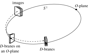
Figure 12: Moving a brane away from an orientifold point.

Chan-Paton symmetry-breaking has an alternative interpretation in terms of D-brane displacements in the dual coordinate space [40, 126]. After a T-duality in the compact dimension, that turns the Neumann boundary condition of the corresponding coordinate into a Dirichlet one, the model lives in a segment $S^{1}/\hbox{\mbm Z}_{2}$, with a pair of O8 planes at its ends. In this description, D8 branes sitting at the two endpoints lead to orthogonal gauge groups, while D8 branes in the interior lead to unitary gauge groups. The previous results can thus be recovered moving the branes from one fixed point to the interior and then to the second fixed point, as shown in figure 12. These phenomena have a natural counterpart in the low-energy effective field theory, where adjoint scalars can acquire vacuum expectation values in the Cartan sub-algebra of the gauge group, compatibly with the vanishing of the corresponding potential, that in the maximally supersymmetric Yang-Mills theory involves only their commutators, and thus preserving supersymmetry. Open strings apparently allow another possibility, breakings via parity-like elements of ${\rm O}(32)$, that as such are not contained in ${\rm SO}(32)$, nor in the ${\rm Spin}(32)/\hbox{\mbm Z}_{2}$ gauge group of the dual heterotic string. An example of this type is the breaking ${\rm SO}(32)\to{\rm SO}(17)\times{\rm SO}(15)$, that does not preserve the overall rank [51], but the duality with the ${\rm Spin}(32)/\hbox{\mbm Z}_{2}$ heterotic string suggests that breakings of this type would lead to inconsistencies in a full non-perturbative treatment [127].

Before leaving the one-dimensional case, it is worth taking a closer look at these amplitudes, noting that $\tilde{\cal K}$ and $\tilde{\cal M}$ involve only even windings, while $\tilde{\cal A}$ involves both even and odd ones. This, however, is not demanded by the reflective conditions at the ends of the tube in the tree channel, that for the two cases are

$${\rm boundary:} \frac{\partial}{\partial\tau}\,X_{L}(\tau-\sigma)=-\,\frac{\partial}{\partial\tau}\,X_{R}(\tau+\sigma)\,,$$

$${\rm crosscap:} \frac{\partial}{\partial\tau}\,X_{L}(\tau-\sigma)=-\,\frac{\partial}{\partial\tau}\,X_{R}(\tau+\sigma+{\textstyle\frac{1}{2}}\pi)\,,$$ (231)

and thus have the same effect on zero modes. Still, the presence of different lattice sums has a sizable consequence: in the $R\to 0$ limit all winding modes collapse to zero mass, and the resulting odd-level tadpoles in $\tilde{\cal A}$ are apparently unmatched. This problem can actually be cured introducing suitable Wilson lines, and to this end let us reconsider eq. (229) for the special case $a=\frac{1}{2}$. In the T-dual picture, as we have seen, this corresponds to placing the branes at the two O8 planes, and

$$\tilde{\cal A}\sim(V_{8}-S_{8})\sum_{n}\frac{\left[N_{1}+N_{2}(-1)^{n}\right]^{2}\;q^{n^{2}R^{2}/4\alpha^{\prime}}}{\eta}\,.$$ (232)

Therefore the choice $N_{1}=N_{2}$, corresponding to the gauge group ${\rm SO}(16)\times{\rm SO}(16)$ removes all odd windings from $\tilde{\cal A}$ and solves the problem of the collapsing tadpoles [128].

There is actually a neater way to understand this result. To this end, let us rewrite $\tilde{\cal K}$ and $\tilde{\cal M}$ in the form [88]

$$\tilde{\cal K} \sim 16^{2}\;(V_{8}-S_{8})\sum_{n}\frac{\left[1+(-1)^{n}\right]^{2}\;q^{n^{2}R^{2}/4\alpha^{\prime}}}{\eta}\,,$$ (233)

$$\tilde{\cal M} \sim -2\times 16\;(\hat{V}_{8}-\hat{S}_{8})\sum_{n}\frac{\left[N_{1}+N_{2}(-1)^{n}\right]\left[1+(-1)^{n}\right]\;q^{n^{2}R^{2}/4\alpha^{\prime}}}{\hat{\eta}}\,.$$

We can now collect all the zero-mode contributions to the three transverse-channel amplitudes in the form

$$\sum_{n}q^{n^{2}R^{2}/4\alpha^{\prime}}\;\left[(16-N_{1})+(16-N_{2})(-1)^{n}\right]^{2}\,,$$ (234)

that shows very clearly how the gauge group ${\rm SO}(16)\times{\rm SO}(16)$ has the unique virtue of eliminating the tadpoles of all winding modes. In the T-dual picture, this configuration corresponds to saturating tadpoles locally at the two ${\rm O}_{+}$ planes, since the cancellation continues to hold in the limit of very large dual radius, when branes away from the orientifolds would move to an infinite distance from them. The phases present in (234) and in the previous amplitudes are indeed Fourier coefficients, that reflect rather clearly the relative positions of these objects on the dual circle.

Repeating the same exercise for the Klein-bottle projection of eq. (219),

$$\tilde{\cal K}\sim 16^{2}\;(V_{8}-S_{8})\sum_{n}\frac{\left[1-(-1)^{n}\right]^{2}\;q^{n^{2}R^{2}/4\alpha^{\prime}}}{\eta}\,,$$ (235)

it is easy to see that in this case the T-dual interval has one ${\rm O}_{+}$ plane and one ${\rm O}_{-}$ plane at its ends. One can again cancel locally the R-R tadpoles, but now placing 16 branes at the ${\rm O}_{+}$ plane and 16 antibranes at the ${\rm O}_{-}$ plane. This configuration, however, breaks supersymmetry, has a dilaton tadpole, and is expected to be unstable, as a result of the net force between branes and antibranes.

We can also reconsider the non-supersymmetric ten-dimensional USp(32) model [79] and study its compactification to $D=9$. We have already seen in subsection 3.2 how in ten dimensions the simultaneous presence of branes and antibranes, corresponding to nonzero values for both $n_{+}$ and $n_{-}$, results in the appearance of tachyonic modes. In the circle reduction, if the radius $R$ is sufficiently small, the tachyonic modes can be lifted by suitable Wilson lines. For instance, a discrete Wilson line, that in the T-dual picture would correspond to placing the (anti)branes at the two ${\rm O}_{-}$-planes, would result in the open spectrum

$${\cal A} = {\textstyle\frac{1}{2}}\sum_{m}\,\left[(n_{+}^{2}+n_{-}^{2})\,(V_{8}-S_{8})\frac{q^{\alpha^{\prime}m^{2}/2R^{2}}}{\eta}\right.$$ (236)

$$\left.+2\,n_{+}n_{-}\,(O_{8}-C_{8})\frac{q^{\alpha^{\prime}(m+1/2)^{2}/2R^{2}}}{\eta}\right]\,,$$

$${\cal M} = {\textstyle\frac{1}{2}}\sum_{m}\,\left[(n_{+}+n_{-})\,\hat{V}_{8}+(n_{-}-n_{+})\,\hat{S}_{8}\right]\frac{q^{\alpha^{\prime}m^{2}/2R^{2}}}{\hat{\eta}}\,,$$ (237)

with $n_{-}-n_{+}=32$, where for the massless modes supersymmetry is again broken by the Möbius projection or, equivalently, by the presence of O_-, rather than O₊, planes. One would therefore expect that supersymmetry be recovered, at least for the massless modes, if a small continuous Wilson line $a$ were introduced in the non-tachyonic model with $n_{+}=0$. In the T-dual picture, this deformation would correspond to moving the antibranes slightly away from the ${\rm O}_{-}$-planes and, indeed, in this case a generic Wilson line would break the original group, USp(32), to U(16), while recovering a global supersymmetry for the massless brane modes. The corresponding amplitudes

$${\cal A} = {\textstyle\frac{1}{2}}(V_{8}-S_{8})\sum_{m}\,\left[2M\bar{M}\;\frac{q^{\alpha^{\prime}m^{2}/2R^{2}}}{\eta}\right.$$ (238)

$$\left.+M^{2}\;\frac{q^{\alpha^{\prime}(m+2a)^{2}/2R^{2}}}{\eta}+\bar{M}^{2}\;\frac{q^{\alpha^{\prime}(m-2a)^{2}/2R^{2}}}{\eta}\right]\,,$$

$${\cal M} = {\textstyle\frac{1}{2}}(\hat{V}_{8}+\hat{S}_{8})\sum_{m}\ \left[M\;\frac{q^{\alpha^{\prime}(m+2a)^{2}/2R^{2}}}{\hat{\eta}}+\bar{M}\;\frac{q^{\alpha^{\prime}(m-2a)^{2}/2R^{2}}}{\hat{\eta}}\right]\,,$$ (239)

display very clearly the phenomenon: the massless modes, unaffected by the Möbius projection, now fill entire vector multiplets.

4.2 Higher-dimensional tori

The compactification on higher-dimensional tori affords even more interesting possibilities. Indeed, aside from richer breaking patterns resulting from continuous Wilson lines, this case allows a peculiar discrete deformation related to the NS-NS antisymmetric tensor $B_{ab}$ [51, 129, 130, 112] . We would like to stress that in the type I superstring the fluctuations of this field are removed by the Klein-bottle projection, but one can nonetheless introduce quantized $B_{ab}$ backgrounds compatible with the symmetry of the type IIB spectrum under the interchange of left and right modes, and then analyse the properties of the corresponding open descendants.

Let us begin by defining, as in [29], the generalizations of $p_{\rm L}$ and $p_{\rm R}$ to a $d$-dimensional torus $T^{d}$:

$$p_{{\rm L},a}=m_{a}+\frac{1}{\alpha^{\prime}}(g_{ab}-B_{ab})\,n^{b}\,,$$ (240)

$$p_{{\rm R},a}=m_{a}-\frac{1}{\alpha^{\prime}}(g_{ab}+B_{ab})\,n^{b}\,.$$ (241)

Here we are slightly changing our notation with respect to the one-dimensional case and to [51], since we are scaling an inverse vielbein out of these momenta, so that the resulting expressions contain only the internal metric. For instance, in this notation the torus amplitude reads

$${\cal T}=|V_{8}-S_{8}|^{2}\ \sum_{m,n}\frac{q^{\frac{\alpha^{\prime}}{4}p_{\rm L}^{T}g^{-1}p_{\rm L}}\ \bar{q}^{\frac{\alpha^{\prime}}{4}p_{\rm R}^{T}g^{-1}p_{\rm R}}}{|\eta(\tau)|^{2d}}\,.$$ (242)

In order to construct the descendants of this compactification, we should make sure that the symmetry $\Omega$ under left-right interchange be still present. It is not hard to convince oneself that this is not possible for generic values of $g_{ab}$ and $B_{ab}$, while one should insist on allowing generic metric deformations, since the corresponding moduli are certainly in the projected spectrum. Hence, the condition that for any pair $(m_{a},n^{a})$ there exist another pair $(m^{\prime}_{b},n^{\prime\,b})$ such that

$$m_{a}+\frac{1}{\alpha^{\prime}}(g_{ab}-B_{ab})\,n^{b}=m^{\prime}_{a}-\frac{1}{\alpha^{\prime}}(g_{ab}+B_{ab})\,{n^{\prime}}^{b}$$ (243)

is to be understood as a constraint on $B_{ab}$, and implies that

$$\frac{2}{\alpha^{\prime}}\,B_{ab}\in\hbox{\mbm Z}\,.$$ (244)

As a result, the independent values for its components are 0 and $\frac{\alpha^{\prime}}{2}$, subject to the condition of antisymmetry. One can then proceed to compute the Klein-bottle amplitude, that is not affected by $B_{ab}$ since it only involves lattice modes with $p_{\rm L}=p_{\rm R}$, and thus with $n^{b}=0$, and for the standard choice of $\Omega$ projection is

$${\cal K}={\textstyle\frac{1}{2}}\,(V_{8}-S_{8})(2i\tau_{2})\ \sum_{m}\frac{q^{\frac{\alpha^{\prime}}{2}m^{T}g^{-1}m}}{\eta^{d}(2i\tau_{2})}\,,$$ (245)

while the corresponding transverse-channel amplitude is

$$\tilde{\cal K}=\frac{2^{5}}{2}\sqrt{{\rm det}(g/\alpha^{\prime})}\ (V_{8}-S_{8})(i\ell)\ \sum_{n}\frac{q^{\frac{1}{\alpha^{\prime}}n^{T}gn}}{\eta^{d}(i\ell)}\,.$$ (246)

The transverse-channel annulus amplitude is to involve contributions from all closed-string states that are paired with their conjugates, where the pairing is determined in this case by the condition of no momentum flow through the ends, $p_{{\rm L},a}=-p_{{\rm R},a}$, as pertains to standard Neumann conditions. The resulting expression does not contain $g_{ab}$ and, given the quantization of $B_{ab}$, becomes a constraint on $n$:

$$\frac{2}{\alpha^{\prime}}\,B_{ab}\,n^{b}=2\,m_{a}\,.$$ (247)

This may be accounted for introducing a projector in the transverse-channel annulus amplitude, that becomes

$$\tilde{\cal A}^{(r)}=\frac{2^{r-d-5}}{2}\,\sqrt{{\rm det}(g/\alpha^{\prime})}\ N^{2}\,(V_{8}-S_{8})(i\ell)\sum_{\epsilon=0,1}\sum_{n}{q^{{1\over 4\alpha^{\prime}}n^{T}gn}\ e^{{2i\pi\over\alpha^{\prime}}n^{T}B\epsilon}\over\eta^{d}(i\ell)}\,,$$ (248)

where the overall factor depending on the rank $r$ of $B_{ab}$ ensures that ${\cal A}$ is properly normalized.

It is worth emphasizing the nature of this expression, since if one substitutes in the bosonic string action the zero modes of eqs. (240) and (241), subject to the condition that only windings flow in the tube, only the first term is generated. Therefore, it is the constraint (247) and not the local dynamics that generates the Wess-Zumino phase, as well as the additional discrete variables $\epsilon_{a}$.

After an $S$ modular transformation, one then obtains the direct-channel annulus amplitude

$${\cal A}^{(r)}=\frac{2^{r-d}}{2}\ N^{2}\,(V_{8}-S_{8})({\textstyle\frac{1}{2}}i\tau_{2})\sum_{\epsilon=0,1}\sum_{m}{q^{{\alpha^{\prime}\over 2}(m+{1\over\alpha^{\prime}}B\epsilon)^{T}g^{-1}(m+{1\over\alpha^{\prime}}B\epsilon)}\over\eta^{d}({\textstyle\frac{1}{2}}i\tau_{2})}\,,$$ (249)

here normalized in such a way that, for any choice of the antisymmetric tensor $B_{ab}$, $N$ is precisely the Chan-Paton multiplicity. This is particularly simple to appreciate in the two limiting cases: for $r=d$ the massless vectors are all obtained when all $\epsilon_{a}=0$, while for $r=0$ all $2^{d}$ values of the $\epsilon_{a}$ contribute.

The Möbius amplitudes

$$\tilde{\cal M}^{(r)} = -\frac{2\times 2^{r/2-d/2}}{2}\,\sqrt{{\rm det}(g/\alpha^{\prime})}\,N\,(\hat{V}_{8}-\hat{S}_{8})(i\ell+{\textstyle\frac{1}{2}})$$ (250)

$$\times\sum_{\epsilon=0,1}\sum_{n}{q^{{1\over\alpha^{\prime}}n^{T}gn}\,\,e^{{2i\pi\over\alpha^{\prime}}n^{T}B\epsilon}\ \gamma_{\epsilon}\over\hat{\eta}^{d}(i\ell+{\textstyle\frac{1}{2}})}$$

and

$$\!\!\!\!\!\!\!\!\!\!{\cal M}^{(r)}=-\frac{2^{r/2-d/2}}{2}N(\hat{V}_{8}-\hat{S}_{8})({\textstyle\frac{1}{2}}i\tau_{2}+{\textstyle\frac{1}{2}})\!\sum_{\epsilon=0,1}\sum_{m}{q^{{\alpha^{\prime}\over 2}(m+{1\over\alpha^{\prime}}B\epsilon)^{T}g^{-1}(m+{1\over\alpha^{\prime}}B\epsilon)}\gamma_{\epsilon}\over\hat{\eta}^{d}({\textstyle\frac{1}{2}}i\tau_{2}+{\textstyle\frac{1}{2}})}$$ (251)

present a new subtlety, since they involve the additional signs $\gamma_{\epsilon}$, needed to ensure a proper normalization of the direct channel compatibly with the tadpole condition, that now becomes

$$\frac{2^{5}}{2}+\frac{2^{r-5}}{2}\;N^{2}+\frac{2\times 2^{r/2-d/2}}{2}\;N\sum_{\epsilon=0,1}\gamma_{\epsilon}=0\,,$$ (252)

and is a perfect square only if

$$\sum_{\epsilon=0,1}\gamma_{\epsilon}=2^{d/2}\,.$$ (253)

As a result, some of the $\gamma$’s must be negative. It should be appreciated that, in general, the resulting gauge group has a reduced rank, since the solution for the Chan-Paton multiplicity $N$ is

$$N=2^{5-r/2}\,.$$ (254)

The $\gamma$’s play a very important rôle also in the direct-channel amplitudes, since they allow one to connect orthogonal and symplectic groups via continuous deformations [51]. In order to illustrate this point, it is instructive to consider in some detail the compactification on a two-torus, whose metric $g_{ab}$ and antisymmetric tensor $B_{ab}$ can be conveniently parametrized in terms of the complex structure $X=X_{1}+iX_{2}$ and of the Kähler structure [10] $Y=Y_{1}+iY_{2}$ as

$$g=\frac{\alpha^{\prime}Y_{2}}{X_{2}}\left(\begin{array}[]{cc}1&X_{1}\\ X_{1}&|X|^{2}\end{array}\right)\,,\qquad B={\alpha^{\prime}}\left(\begin{array}[]{cc}0&Y_{1}\\ -Y_{1}&0\end{array}\right)\,,$$ (255)

where the independent values for $Y_{1}$ are 0 and ${1\over 2}$. In section 2 we have already met the complex structure of the world-sheet torus, the “shape” of the corresponding parallelogram, and here $X$ describes in a similar fashion the “shape” of the target-space torus. The imaginary part of the Kähler structure has also a very simple interpretation: up to a normalization, it is the area of the target-space torus.

For the interesting case $Y_{1}={1\over 2}$, that corresponds to $r=2$, the annulus amplitudes are

$$\tilde{\cal A}^{(2)} = \frac{2^{-5}N^{2}}{2}\ Y_{2}\ (V_{8}-S_{8})$$ (256)

$$\times\sum_{n_{1},n_{2}}\frac{W_{n_{1},n_{2}}\left[1+(-1)^{n_{1}}+(-1)^{n_{2}}+(-1)^{n_{1}+n_{2}}\right]}{\eta^{2}}\,,$$

$${\cal A}^{(2)}={\textstyle\frac{1}{2}}\,N^{2}\ (V_{8}-S_{8})\ \frac{\left[P_{0,0}+P_{-\frac{1}{2},0}+P_{0,\frac{1}{2}}+P_{-\frac{1}{2},\frac{1}{2}}\right]}{\eta^{2}}\,,$$ (257)

and, in a similar fashion, the Möbius amplitudes are

$$\tilde{\cal M}^{(2)} = -{\textstyle\frac{2}{2}}\,N\ Y_{2}\ (\hat{V}_{8}-\hat{S}_{8})\frac{1}{\hat{\eta}^{2}}\sum_{n_{1},n_{2}}W_{2n_{1},2n_{2}}$$ (258)

$$\times\left[\gamma_{0,0}+(-1)^{n_{1}}\gamma_{0,1}+(-1)^{n_{2}}\gamma_{1,0}+(-1)^{n_{1}+n_{2}}\gamma_{1,1}\right]\,,$$

$${\cal M}^{(2)} = -{\textstyle\frac{1}{2}}\,N\ (\hat{V}_{8}-\hat{S}_{8})$$ (259)

$$\times\frac{\left[\gamma_{0,0}P_{0,0}+\gamma_{0,1}P_{-\frac{1}{2},0}+\gamma_{1,0}P_{0,\frac{1}{2}}+\gamma_{1,1}P_{-\frac{1}{2},\frac{1}{2}}\right]}{\hat{\eta}^{2}}\,,$$

where we have introduced a compact notation for the winding and momentum sums:

$$W_{n_{1},n_{2}} = q^{\frac{Y_{2}}{4X_{2}}[(n_{1}+X_{1}n_{2})^{2}+n_{2}^{2}X_{2}^{2}]}\,,$$

$$P_{\epsilon_{1},\epsilon_{2}} = \sum_{m_{1},m_{2}}q^{\frac{1}{2X_{2}Y_{2}}[(m_{2}-\epsilon_{2}-X_{1}(m_{1}-\epsilon_{1}))^{2}+(m_{1}-\epsilon_{1})^{2}X_{2}^{2}]}\,.$$ (260)

One can easily extract the contributions of the three amplitudes to the R-R tadpole,

$$\tilde{\cal K} \to -2^{5}\,,$$

$$\tilde{\cal A}^{(2)} \to -2^{-5}\times N^{2}\times 4\,,$$

$$\tilde{\cal M}^{(2)} \to 2\times N\times(\gamma_{0,0}+\gamma_{0,1}+\gamma_{1,0}+\gamma_{1,1})\,,$$ (261)

and it is evident that, in order to solve the tadpole condition, one of the four $\gamma_{\epsilon}$ is to equal minus one, while the three others are to equal plus one. As a result, the total charge is reduced, consistently with the rank reduction for the Chan-Paton gauge group. Among the four possible choices, only two lead to different results, depending on the sign of $\gamma_{0,0}$. If $\gamma_{0,0}=+1$, the massless open-string vector is in the adjoint of ${\rm SO}(16)$, while if $\gamma_{0,0}=-1$ it is in the adjoint of ${\rm USp}(16)$. Notice that a T-duality along both internal coordinates would actually alter the $\Omega$ projection, moving the restriction to even windings from $\tilde{\cal A}$ to ${\cal K}$ [53], as we shall see in detail in the next section.

As anticipated, orthogonal and symplectic gauge groups can be connected via continuous Wilson lines. As an example, let us consider the compactification on the two-dimensional torus with a Wilson line in the 1 direction. For definiteness, let us choose $\gamma_{0,0}=-1$, $\gamma_{1,0}=\gamma_{1,1}=\gamma_{0,1}=1$, so that the annulus and Möbius amplitudes in the transverse channel are

$$\tilde{\cal A}^{(2)} = \frac{2^{-5}}{2}\ Y_{2}\ (V_{8}-S_{8})\sum_{n_{1},n_{2}}\left(Me^{2i\pi an_{1}}+\bar{M}e^{-2i\pi an_{1}}\right)^{2}$$ (262)

$$\times\frac{W_{n_{1},n_{2}}\left[1+(-1)^{n_{1}}+(-1)^{n_{2}}+(-1)^{n_{1}+n_{2}}\right]}{\eta^{2}}$$

and

$$\tilde{\cal M}^{(2)} = {\textstyle\frac{2}{2}}\ Y_{2}\ (V_{8}-S_{8})\frac{1}{\eta^{2}}\sum_{n_{1},n_{2}}W_{2n_{1},2n_{2}}$$ (263)

$$\times\left(Me^{4i\pi an_{1}}+\bar{M}e^{-4i\pi an_{1}}\right)$$

$$\times\left[1-(-1)^{n_{1}}-(-1)^{n_{2}}-(-1)^{n_{1}+n_{2}}\right]\,,$$

while the usual rescalings and the $S$ and $P$ modular transformations give

$${\cal A}^{(2)} = {\textstyle\frac{1}{2}}\ (V_{8}-S_{8})\ \frac{1}{\eta^{2}}\Biggl{\{}2M\bar{M}\left[P_{0,0}+P_{\frac{1}{2},0}+P_{0,\frac{1}{2}}+P_{\frac{1}{2},\frac{1}{2}}\right]$$ (264)

$$+M^{2}\ \left[P_{2a,0}+P_{2a+\frac{1}{2},0}+P_{2a,\frac{1}{2}}+P_{2a+\frac{1}{2},\frac{1}{2}}\right]$$

$$+\bar{M}^{2}\ \left[P_{-2a,0}+P_{-2a+\frac{1}{2},0}+P_{-2a,\frac{1}{2}}+P_{-2a+\frac{1}{2},\frac{1}{2}}\right]\Biggr{\}}$$

for the annulus amplitude, and

$${\cal M}^{(2)} = {\textstyle\frac{1}{2}}\ (V_{8}-S_{8})\frac{1}{\eta^{2}}$$

$$\times\Biggl{\{}M\left[P_{2a,0}-P_{2a+\frac{1}{2},0}-P_{2a,\frac{1}{2}}-P_{2a+\frac{1}{2},\frac{1}{2}}\right]$$

$$+\bar{M}\left[P_{-2a,0}-P_{-2a+\frac{1}{2},0}-P_{-2a,\frac{1}{2}}-P_{-2a+\frac{1}{2},\frac{1}{2}}\right]\Biggr{\}}$$

for the Möbius amplitude. For a generic Wilson line $a$, with $0\leq a<\frac{1}{2}$, the gauge group is thus U(8), but for $a=0$ the lattice sums $P_{\pm 2a,0}$ contribute massless modes to ${\cal A}$ and ${\cal M}$, and the gauge group enhances to USp(16). On the other hand, for $a=\frac{1}{4}$ the lattice sums $P_{\pm 2a+\frac{1}{2},0}$ contribute massless modes, and since these terms are accompanied in ${\cal M}$ by additional signs, the gauge group enhances to SO(16). The Wilson line is a modulus of the compactified open string, and therefore orthogonal and symplectic gauge groups are indeed continuously connected [51].

4.3 T-duality and discrete moduli

It is instructive to study a bit further the effect of T-duality on toroidally compactified type I strings. This subject was originally considered in [39, 40, 41], and, as we have seen, results in an equivalent, though rather pervasive, description of gauge symmetry breaking by Wilson lines, momentum-space translations, in terms of spatial displacements of the extended objects where the ends of open strings terminate.

In order to appreciate the effect of T-duality on the construction of open descendants, one can begin by observing, as in subsection 4.1, that the circle inversion $R\to{\alpha^{\prime}}/{R}$ turns quantized momenta $p\sim 1/R$ into windings $w\sim R/\alpha^{\prime}$. These, on the other hand, can only be supported by open strings whose ends are fixed. Therefore, the T-dual picture of an open string with Neumann boundary conditions involves a novel type of string with Dirichlet boundary conditions [39, 40, 41, 126], and this poses the problem of the identity of the hyper-surfaces where the ends live. In fact, T-duality is a world-sheet duality transformation that interchanges $\sigma$ and $\tau$, and thus tangential and normal derivatives. At a boundary, where the original Neumann condition was turning $X_{\rm L}$ into $X_{\rm R}$, the left and right modes of a closed string, the Dirichlet condition generated by T-duality turns $X_{\rm L}$ into $-X_{\rm R}$. In this sense T-duality acts as a parity transformation, but, say, limitedly to the right-moving modes, and this provides a consistent picture of the whole construction. To begin with, the direct-channel Klein-bottle amplitude now involves only winding modes, that are precisely fixed by the combination of the usual world-sheet parity $\Omega$ with the inversion of the right-moving modes, $X_{\rm L}\leftrightarrow-X_{\rm R}$. In addition, the open-string coordinate involves an expansion in terms of $\sin(n\sigma)$, that can also be associated to the new way of combining left and right modes.

Open strings thus terminate on extended objects, D-branes, whose dimensions are altered by T-duality transformations [126]. In particular, Neumann strings can be thought of as terminating on D9 branes, that invade the whole ten-dimensional space-time, and that T-duality along any of the coordinates turns into D8 branes. In a similar fashion, the ends of a string with $p+1$ Neumann boundary conditions and $9-p$ Dirichlet boundary conditions live on a D$p$ brane, and, more generally, a T-duality increases or reduces the dimension of a D-brane according to whether it involves a direction orthogonal or parallel to it.

An additional feature of D-branes and O-planes that has attracted much attention during the last few years is their tension. Since they both show up in two genus-${1\over 2}$ world-sheets, the disk and the projective plane, they are naturally weighted by a factor $1/g_{s}$, a rather peculiar feature when compared to ordinary solitons, whose mass scales like $1/g^{2}$, with $g$ a typical coupling of a gauge theory [62].

This cursory review of T-duality suffices to bring us to our next topic. In the previous section we have seen how quantized values of the NS-NS tensor $B_{ab}$ play an important rôle in the vacuum amplitudes for Neumann strings. We can now describe how different orientifold projections can result in quantized values for other moduli of the “parent” closed string [132]. For simplicity, we shall concentrate on the $T^{2}$ case, but similar results apply to higher-dimensional tori.

On $T^{2}$ one has the two distinct options of performing a T-duality along both coordinates or along a single one. The first, discussed in the previous subsection, can replace the ${\rm O}9_{+}$ plane with three ${\rm O}7_{+}$ and one ${\rm O}7_{-}$, but $B_{ab}$ remains a discrete deformation. On the other hand, a T-duality along a single direction combines the $\Omega$ projection with the conjugation ${\cal R}:\ Z_{\rm R}\to\bar{Z}_{\rm R}$ of the complex right-moving coordinate $Z_{\rm R}=(X^{7}_{\rm R}+iX^{8}_{\rm R})/\sqrt{2}$ on the target $T^{2}$, and a simple analysis of the massless spectrum reveals that in this case the internal components of the NS-NS antisymmetric tensor

$$\left(\psi_{-{1\over 2}}^{1}\tilde{\psi}_{-{1\over 2}}^{2}-\psi_{-{1\over 2}}^{2}\tilde{\psi}_{-{1\over 2}}^{1}\right)|0\tilde{0}\rangle$$

survive the $\Omega{\cal R}$ projection, while the mixed components of the internal metric

$$\left(\psi_{-{1\over 2}}^{1}\tilde{\psi}_{-{1\over 2}}^{2}+\psi_{-{1\over 2}}^{2}\tilde{\psi}_{-{1\over 2}}^{1}\right)|0\tilde{0}\rangle$$

do not. Therefore, in this case the antisymmetric tensor is a continuous modulus of the projected theory, while some quantization condition should be met by the mixed components of the metric. Indeed, from the expressions

$$p_{\rm L} = {1\over\sqrt{\alpha^{\prime}X_{2}Y_{2}}}\left[-Xm_{1}+m_{2}+\bar{Y}(n_{1}+Xn_{2})\right]\,,$$

$$p_{\rm R} = {1\over\sqrt{\alpha^{\prime}X_{2}Y_{2}}}\left[-Xm_{1}+m_{2}+Y(n_{1}+Xn_{2})\right]\,,$$

for the left and right complex momenta on a $T^{2}$ with complex structure $X$ and Kähler form $Y$, whose metric and antisymmetric tensor are given in eq. (255), one can see that requiring the invariance of the parent theory under

$$\Omega{\cal R}:\qquad p_{\rm L}\leftrightarrow\bar{p}_{\rm R}$$ (265)

results in a quantization condition for the real slice of the complex structure, so that now $2X_{1}\in\hbox{\mbm Z}$. This is to be compared with the standard case, discussed previously, where the quantization condition applied to the real slice $B_{ab}$ of the Kähler form.

The closed-string states allowed in the transverse-channel amplitudes $\tilde{\cal A}$ and $\tilde{\cal M}$ are now subject to the constraints

$$2X_{1}m_{1}\,,\ 2X_{1}n_{2}\in 2\hbox{\mbm Z}\,,$$ (266)

that, as in the standard case, result in the insertion of suitable projectors in the annulus and Möbius amplitudes. For half-integer values of $X_{1}$, these have the effect of halving the Chan-Paton multiplicities. We have thus met a generic feature of open descendants: non-vanishing, quantized, backgrounds for the closed-string moduli eliminated by the orientifold projection typically reduce the rank of the Chan-Paton gauge group.

In this example, the open descendants with conventional $\Omega$ projection are effectively constructed on the mirror torus, where the rôles of $X$ and $Y$ are interchanged, so that now $Y$ and $X$ are the complex and Kähler structures. This correspondence is well known from closed strings: on a $T^{2}$, T-duality along a one-cycle is indeed the simplest instance of a mirror symmetry [133].

A rank reduction similar to that induced in open-string models by a quantized $B_{ab}$ manifests itself also in the heterotic models usually termed CHL strings [134], where it originates from higher-level realizations of the current algebra. There is indeed a nice duality correspondence between these two classes of models, first noticed in [130, 112].

5 Orbifold compactification

Since their first appearance in [28], toroidal orbifolds have proved a major source of insight into the structure of String Theory. In the resulting wide class of exactly solvable models, strings propagate consistently in singular curved spaces and display rich patterns of interesting low-energy spectra.

Orbifolds can be constructed subjecting smooth covering manifolds to discrete identifications. These in general leave some sets of points fixed, that as a result support curvature singularities. Whereas in such singular spaces the dynamics of particles is generally ill-defined, modular invariance fully determines the resulting spectra for oriented closed strings. These include an “untwisted” sector, whose states are subsets of those present in the covering manifolds, and additional “twisted” sectors confined to the fixed points. Typically, the latter also include some blow-up moduli, capable of lifting the orbifold singularities, thus connecting these spaces to nearby smooth manifolds.

This section is devoted to orbifold compactifications of models with open strings. We begin by considering the bosonic string on the one-dimensional orbifold of a circle, that allows one to describe the rôle of Neumann and Dirichlet boundary conditions in a relatively simple setting. We then move on to one-dimensional shift orbifolds of the type-I superstring, the simplest models where the breaking of supersymmetry is related to a continuous parameter, the radius $R$ of a circle. Six-dimensional supersymmetric open-string models display new types of low-energy spectra, that generally contain several tensor multiplets, and are thus vastly different from heterotic models. In orbifold compactifications, the rank reduction induced by a quantized $B_{ab}$, familiar from the toroidal case of section 4, is accompanied by a grouping of the fixed points, that results in the presence of several tensor multiplets in the closed sector and of several families of ND states in the open sector. Six-dimensional orbifolds are also the simplest examples whose consistency can require that supersymmetry be broken on branes. All these aspects are reviewed in some detail, before describing the simplest chiral four-dimensional supersymmetric model, the open descendant of the $T^{6}/\hbox{\mbm Z}_{3}$ IIB compactification, whose spectrum includes three families of chiral matter. “Brane supersymmetry breaking” provides also the solution to an interesting class of otherwise inconsistent four-dimensional models, associated to $\hbox{\mbm Z}_{2}\times\hbox{\mbm Z}_{2}$ orbifolds, that we then review in some detail before turning to a discussion of magnetic deformations. We conclude with a cursory view of the D-branes present in the ten-dimensional strings and in their orientifolds.

5.1 The one-dimensional orbifold of the bosonic string

Let us begin by considering the one-dimensional orbifold of the bosonic string, whose open descendants were first constructed in [42]. The starting point is the torus amplitude (65), now projected in order to retain only states built by operators invariant under the internal parity $X^{25}\to-X^{25}$. This is achieved combining the original internal lattice operators, with $P_{\rm L,R}$ defined in (214), into pairs of definite parity, that can then be accompanied by even or odd powers of string oscillators according to

$$\prod_{i,j}\;{\alpha_{-n_{i}}^{25}\,\tilde{\alpha}_{-n_{j}}^{25}}\;\cos(p_{\rm L}X_{\rm L}+p_{\rm R}X_{\rm R}) \quad{\rm for}\quad \#(i+j)\in 2\hbox{\mbm Z}\,,$$ (267)

$$\prod_{i,j}\;{\alpha_{-n_{i}}^{25}\,\tilde{\alpha}_{-n_{j}}^{25}}\;\sin(p_{\rm L}X_{\rm L}+p_{\rm R}X_{\rm R}) \quad{\rm for}\quad \#(i+j)\in 2\hbox{\mbm Z}+1\,,$$ (268)

since $(-1)^{\#(i+j)}$, with ${\#(i+j)}$ the total number of oscillators in the vertices, is the overall parity of these oscillator modes. Hence, away from the origin of the lattice, the operators that survive the projection are simply half of those allowed in the covering torus, while an additional contribution is needed to count properly the remaining ones, that have $p_{\rm L}=0=p_{\rm R}$. All this is neatly encoded in the “untwisted” partition function

$${\cal T}_{\rm(u)}={\textstyle\frac{1}{2}}\;\sum_{m,n}\frac{q^{\alpha^{\prime}p_{\rm L}^{2}/4}\;\bar{q}^{\alpha^{\prime}p_{\rm R}^{2}/4}}{\eta(\tau)\eta(\bar{\tau})}+{\textstyle\frac{1}{2}}\;\left|\frac{2\eta}{\vartheta_{2}}\right|\,,$$ (269)

where, for the sake of brevity, we are omitting the factors $1/(\sqrt{\tau_{2}}\eta\bar{\eta})$ associated to the remaining non-compact transverse coordinates. The second contribution is not invariant under the $S$ modular transformation, while its $S$-transform is not invariant under the $T$ transformation. Still, combining all these terms gives a modular invariant partition function, that describes the propagation of the closed bosonic string on the segment $S^{1}/\hbox{\mbm Z}_{2}$:

$${\cal T}={\textstyle\frac{1}{2}}\;\sum_{m,n}\frac{q^{\alpha^{\prime}p_{L}^{2}/4}\;\bar{q}^{\alpha^{\prime}p_{R}^{2}/4}}{\eta(\tau)\eta(\bar{\tau})}+{\textstyle\frac{1}{2}}\;\left|\frac{2\eta}{\vartheta_{2}}\right|+{\textstyle\frac{2}{2}}\;\left|\frac{\eta}{\vartheta_{4}}\right|+{\textstyle\frac{2}{2}}\;\left|\frac{\eta}{\vartheta_{3}}\right|\,.$$ (270)

In the last two terms, that define the “twisted” sector, the overall factor of two is fixed by the modular invariance of ${\cal T}$, and accounts for the two sectors living at the orbifold fixed points.

As in previous examples, the open descendants are built halving ${\cal T}$ and adding the corresponding Klein-bottle amplitude. Following [42], we begin by confining our attention to the simplest choice,

$${\cal K}={\textstyle\frac{1}{4}}\;\sum_{m}\frac{q^{\frac{\alpha^{\prime}}{2}\left(\frac{m}{R}\right)^{2}}}{\eta(2i\tau_{2})}+{\textstyle\frac{1}{4}}\;\sum_{n}\frac{q^{\frac{1}{2\alpha^{\prime}}(nR)^{2}}}{\eta(2i\tau_{2})}+{\textstyle\frac{2}{2}}\sqrt{\frac{\eta}{\vartheta_{4}}}\,.$$ (271)

In order to justify this expression, let us begin by noting that there are two subsets of the untwisted cosine-operators in (267) that are fixed under the involution $\Omega$, and thus contribute to ${\cal K}$. Aside from the terms with zero winding, that we already met in the previous section, the even nature of the cosine vertices also fixes the operators with zero momentum, whose argument is odd under $\Omega$. Finally, the last term in eq. (271) is associated to the twisted states, and has the proper multiplicity to account for the two fixed points. Notice that this expression does not involve the two functions $\vartheta_{2}$ and $\vartheta_{3}$, that would reflect an antiperiodic behaviour under vertical transport in the doubly-covering torus. This can be clearly seen from the geometry of the Klein bottle in fig. 5: in this example the orbifold involution relating pairs of image points is $\hbox{\mbm Z}_{2}$ valued, and for consistency must square to a periodic vertical translation on the covering torus.

An equivalent description of this spectrum exhibits its orthogonal decomposition in different sectors [135]. It is rather effective and explicit for the oscillator excitations at the origin of the lattice, for which one can define the four combinations

$$\phi_{+\pm}={\textstyle\frac{1}{2}}\left(\;\frac{1}{\eta}\pm\sqrt{\frac{2\eta}{\vartheta_{2}}}\;\right)\,,\qquad\phi_{-\pm}={\textstyle\frac{1}{2}}\left(\;\sqrt{\frac{\eta}{\vartheta_{4}}}\pm\sqrt{\frac{\eta}{\vartheta_{3}}}\;\right)\,,$$ (272)

and in terms of these expressions the torus partition function becomes

$${\cal T}=|\phi_{++}|^{2}+|\phi_{+-}|^{2}+2|\phi_{-+}|^{2}+2|\phi_{--}|^{2}+{\textstyle\frac{1}{2}}\;\sum{}^{\prime}\,.$$ (273)

The primed sum refers to the operators associated to points of the lattice away from the origin that, as we have seen, combine in pairs, and whose $\hbox{\mbm Z}_{2}$ symmetrization is properly accounted for by the overall factor ${1\over 2}$. Actually, each of the twisted terms is not a full specification of the corresponding operators, since we are unable to distinguish in ${\cal T}$ pairs of operators that belong to different fixed points. From the conformal field theory viewpoint, we are thus facing an ambiguity, but the structure is nonetheless evident, and indeed the Klein-bottle amplitude reads

$${\cal K}={\textstyle\frac{1}{2}}\;\left[\phi_{++}+\phi_{+-}+2\phi_{-+}+2\phi_{--}+{\textstyle\frac{1}{2}}\;(P^{\prime}_{m}+W^{\prime}_{n})\right]\,,$$ (274)

where the complete momentum and winding sums present in ${\cal K}$ and in the annulus amplitude ${\cal A}$ that we shall introduce shortly are

$$P_{m}(q^{\gamma})=\sum_{m}\;\frac{q^{\frac{\alpha^{\prime}}{2}\left(\frac{m}{R}\right)^{2}}}{\eta(q^{\gamma})}\,,\qquad W_{n}(q^{\gamma})=\sum_{n}\;\frac{q^{\frac{(nR)^{2}}{2\alpha^{\prime}}}}{\eta(q^{\gamma})}\,,$$ (275)

with $\gamma=2$ for ${\cal K}$ and $\gamma=1/2$ for ${\cal A}$, while the “primed” sums lack the terms at the origin of the lattices. Eq. (274) reflects precisely our previous comments, and may thus be regarded as an alternative justification for (271).

We can now turn ${\cal K}$ to the transverse channel, by an $S$ modular transformation. Taking into account the contributions of the remaining non-compact coordinates, in terms of the modulus of the double cover the result is

$$\tilde{\cal K}=\frac{2^{13}}{4}\;\left[v\;W_{2n}+\frac{1}{v}\;P_{2n}+2\sqrt{\frac{2\eta}{\vartheta_{2}}}\right]\,,$$ (276)

where, in order to lighten the notation, we have introduced the dimensionless radius, $v=R/\sqrt{\alpha^{\prime}}$. In terms of the $\phi$’s this expression becomes

$$\tilde{\cal K} = \frac{2^{13}}{2}\;\left[\left(\sqrt{v}+\frac{1}{\sqrt{v}}\right)^{2}\phi_{++}\right.$$ (277)

$$+\left.\left(\sqrt{v}-\frac{1}{\sqrt{v}}\right)^{2}\phi_{+-}+v\;W^{\prime}_{2n}+\frac{1}{v}\;P^{\prime}_{2n}\right]\,,$$

where the zero modes exhibit very clearly the familiar structure of perfect squares for the reflection coefficients.

The open sector is quite interesting, since on this $\hbox{\mbm Z}_{2}$ orbifold it allows for the simultaneous presence of open strings with different boundary conditions. Aside from the standard strings with Neumann conditions at their two ends, NN strings, additional ones, DD and ND, with Dirichlet-Dirichlet and mixed Neumann-Dirichlet boundary conditions are present, together with their $\hbox{\mbm Z}_{2}$ orbifold projections. These different types of strings have by now a geometrical interpretation in terms of bosonic D25 and D24 branes, while the annulus amplitude reads

$${\cal A} = {\textstyle{1\over 4}}\left[N^{2}\;P_{m}+D^{2}\;W_{n}+\left(R_{N}^{2}+R_{D}^{2}\right)\sqrt{2\eta\over\vartheta_{2}}\right.$$ (278)

$$+2\,\left.N\,D\;\sqrt{\eta\over\vartheta_{4}}+2\,R_{N}\,R_{D}\;\sqrt{\eta\over\vartheta_{3}}\right]\,.$$

Here $N$ and $D$ count the overall numbers of D25 and D24 branes, while $R_{N}$ and $R_{D}$ encode the $\hbox{\mbm Z}_{2}$ orbifold action on the corresponding Chan-Paton charges. The first term involves a sum over Kaluza-Klein momenta, and thus refers to NN strings, whose ends live on D25 branes. On the other hand, the winding contribution refers to DD strings, whose ends are free to move in the 24 non-compact dimensions, parallel to the D24 branes, but are fixed in the compact one. For simplicity we have only considered DD strings at a single fixed point of the $S^{1}/\hbox{\mbm Z}_{2}$ orbifold, but more general configurations, where the D24 branes are distributed between the fixed points or moved to the bulk of the compact space, are also possible. We shall return to this option in the following sections. Finally, open strings with mixed ND boundary conditions, i.e. stretched between D25 and D24 branes, have half-integer mode expansions and an additional factor of two that reflects the two orientations of their endpoints.

The Möbius amplitude receives contributions only from NN and DD strings, and reads

$${\cal M}={\textstyle{1\over 4}}\,\epsilon\,\left[N\,\hat{P}_{m}+D\,\hat{W}_{n}+(N+D)\sqrt{2\hat{\eta}\over\hat{\vartheta}_{2}}\right]\,,$$ (279)

where $\epsilon$ is an overall sign. It can be recovered, as usual, from the corresponding transverse-channel amplitude $\tilde{\cal M}$, determined by the factorization of $\tilde{\cal K}$ and $\tilde{\cal A}$.

In superstring vacua the new type of boundary condition is generally not optional, but is demanded by R-R tadpole cancellations, and thus by space-time anomalies [35]. A closer look at $\tilde{\cal K}$ reveals also in this case the existence of two types of tadpoles. These can be associated to the standard bosonic O25 planes, whose contribution scales proportionally to the length of the circle, consistently with the fact that they invade the whole internal space, and to new bosonic O24 planes, whose contribution scales inversely with it, consistently with the fact that they are localized at the two fixed points. Thus, both D25 and D24 branes would be needed in this case if one insisted on cancelling all tadpoles, as can be seen from the transverse-channel open-string amplitudes

$$\tilde{\cal A} = {2^{-13}\over 4}\Biggl{[}N^{2}\,v\,W_{n}+{D^{2}\over v}\,P_{n}+2\,N\,D\sqrt{2\eta\over\vartheta_{2}}$$ (280)

$$+2\left(R^{2}_{N}+R^{2}_{D}\right)\sqrt{\eta\over\vartheta_{4}}+2\,\sqrt{2}\,R_{N}\,R_{D}\,\sqrt{\eta\over\vartheta_{3}}\Biggr{]}$$

and

$$\tilde{\cal M}={\textstyle{2\over 4}}\,\epsilon\,\left[N\,v\,W_{2n}+{D\over v}\,P_{2m}+(N+D)\sqrt{2\hat{\eta}\over\hat{\vartheta}_{2}}\right]\,,$$ (281)

that in terms of the $\phi$’s would become

$$\tilde{\cal A} = {2^{-13}\over 4}\Biggl{\{}\left(N\sqrt{v}+{D\over\sqrt{v}}\right)^{2}\,\phi_{++}$$ (282)

$$+\left(N\sqrt{v}-{D\over\sqrt{v}}\right)^{2}\,\phi_{+-}$$

$$+2\,\left[\left({R_{N}\over\sqrt{2}}+R_{D}\right)^{2}+\left({R_{N}\over\sqrt{2}}\right)^{2}\right]\,\phi_{-+}$$

$$+2\,\left[\left({R_{N}\over\sqrt{2}}-R_{D}\right)^{2}+\left({R_{N}\over\sqrt{2}}\right)^{2}\right]\,\phi_{--}\Biggr{\}}+\ldots$$

and

$$\tilde{\cal M} = {\textstyle{2\over 4}}\,\epsilon\,\Biggl{[}\left(\sqrt{v}+{1\over\sqrt{v}}\right)\left(N\sqrt{v}+{D\over\sqrt{v}}\right)\,\hat{\phi}_{++}$$ (283)

$$+\left(\sqrt{v}-{1\over\sqrt{v}}\right)\left(N\sqrt{v}-{D\over\sqrt{v}}\right)\,\hat{\phi}_{+-}\Biggr{]}+\ldots\,.$$

These expressions match precisely the Klein-bottle amplitude (277), while the tadpole conditions would lead to

$$N =-\,8192\,\epsilon\,,\qquad\quad R_{N} =0\,,$$

$$D =-\,8192\,\epsilon\,,\qquad\quad R_{D} =0\,,$$ (284)

thus also requiring that $\epsilon=-1$.

We would like to stress that the amplitude (282) reveals rather neatly the geometry of the D-brane configuration: not only do $N$ and $D$ count the overall numbers of D25 and D24 branes, but the twisted terms clearly display that only one of the two fixed points accommodates all the D24 branes.

To conclude our description of the $S^{1}/\hbox{\mbm Z}_{2}$ orbifold, we now turn to the open spectrum, rewriting also ${\cal A}$ and ${\cal M}$ in terms of the $\phi$’s. The result is

$${\cal A}_{0} \sim {\textstyle{1\over 4}}\Bigl{\{}\left[(N^{2}+R_{N}^{2})+(D^{2}+R_{D}^{2})\right]\,\phi_{++}$$ (285)

$$+\left[(N^{2}-R_{N}^{2})+(D^{2}-R_{D}^{2})\right]\,\phi_{+-}$$

$$+2\left(N\,D+R_{N}\,R_{D}\right)\phi_{-+}+2\left(N\,D+R_{N}\,R_{D}\right)\phi_{--}\Bigr{\}}$$

for the annulus amplitude, and

$${\cal M}_{0}\sim{\textstyle{1\over 2}}\,\epsilon\,(N+D)\,\phi_{++}$$ (286)

for the Möbius amplitude. A consistent particle interpretation of the direct-channel amplitudes calls for a regular action of the $\hbox{\mbm Z}_{2}$ orbifold group on the charge space, and thus for a parametrization in terms of “real” Chan-Paton multiplicities, so that

$$N =n_{1}+n_{2}\,,\qquad\quad R_{N} =n_{1}-n_{2}\,,$$

$$D =d_{1}+d_{2}\,,\qquad\quad R_{D} =d_{1}-d_{2}\,,$$ (287)

Enforcing the tadpole conditions (284), this would result in a gauge group comprising two copies of ${\rm SO}(4096)\times{\rm SO}(4096)$, associated to D25 and D24 branes respectively, with tachyons in symmetric representations and scalars in bi-fundamentals.

5.2 The one-dimensional shift-orbifold

We now turn to orbifold compactifications of the type I superstring where the target-space coordinates are not identified under reflections, as in the previous case, but under discrete, fractional, shifts of the lattice basis vectors or, more generally, under the combined action of shifts and internal symmetries. This combined action is particularly interesting, since it can implement in String Theory [76] the Scherk-Schwarz mechanism [67] to attain the breaking of supersymmetry. In the simplest case of circle compactification, this allows higher-dimensional modes that are periodic only up to an internal symmetry transformation. The Kaluza-Klein momenta of the various fields are thus shifted proportionally to their charges, with the consequent possibility of introducing mass differences between bosons and fermions.

In Field Theory, with only Kaluza-Klein excitations available, the Scherk-Schwarz mechanism can only result from shifts of internal momenta. On the other hand, String Theory offers more possibilities, since one has also the option of affecting the windings. For oriented closed superstrings these two deformations, related by T-duality, describe essentially the same phenomenon. After orientifolding, however, they lead to completely different results. As in [69], we shall refer to these two mechanisms as Scherk-Schwarz and M-theory breaking, since the second can actually be related via string dualities to conventional Scherk-Schwarz deformations along the eleventh coordinate. In the latter case we shall also meet an interesting phenomenon, “brane supersymmetry”, where this appropriate term was actually coined in [136]: the low-lying excitations of a brane immersed in a non-supersymmetric bulk can be supersymmetric. This phenomenon is generic and, as we shall see, admits a neat geometrical interpretation. Orientifolds of this type with partial breaking of supersymmetry were first discussed in [70], while in more complicated models even entire towers of brane excitations can be supersymmetric [71].

5.3 Momentum shifts: Scherk-Schwarz supersymmetry breaking

Let us begin by describing the effect of momentum deformations [68, 69]. As we shall see, in this case the open sector will involve branes that fill the compactified dimension, and are thus affected by the Scherk-Schwarz deformation. These models can be realized via freely-acting orbifolds, projecting the IIB superstring with the $\hbox{\mbm Z}_{2}$ generator $(-1)^{F}\,\delta$, where $F=F_{{\rm L}}+F_{{\rm R}}$ is the total space-time fermion number and $\delta$ is the shift $x^{9}\to x^{9}+\pi R$ along the ninth spatial dimension, a circle of radius $R$. The resulting torus partition function is

$${\cal T}_{{\rm KK}} = {\textstyle{1\over 2}}\Biggl{[}|V_{8}-S_{8}|^{2}\;\Lambda_{m,n}+|V_{8}+S_{8}|^{2}\;(-1)^{m}\Lambda_{m,n}$$ (288)

$$+|O_{8}-C_{8}|^{2}\;\Lambda_{m,n+{1\over 2}}+|O_{8}+C_{8}|^{2}\;(-1)^{m}\Lambda_{m,n+{1\over 2}}\Biggr{]}\,,$$

where, for brevity, we have let

$$\Lambda_{m+a,n+b}={q^{{\alpha^{\prime}\over 4}\left({(m+a)\over R}+{(n+b)R\over\alpha^{\prime}}\right)^{2}}\;\bar{q}^{{\alpha^{\prime}\over 4}\left({(m+a)\over R}-{(n+b)R\over\alpha^{\prime}}\right)^{2}}\over\eta(q)\,\eta(\bar{q})}\,,$$ (289)

while leaving all lattice sums implicit. Expanding the various terms in ${\cal T}_{{\rm KK}}$ then yields the orthogonal decomposition of the spectrum

$${\cal T}_{{\rm KK}} = (V_{8}\bar{V}_{8}+S_{8}\bar{S}_{8})\Lambda_{2m,n}+(O_{8}\bar{O}_{8}+C_{8}\bar{C}_{8})\Lambda_{2m,n+{1\over 2}}$$ (290)

$$-(V_{8}\bar{S}_{8}+S_{8}\bar{V}_{8})\Lambda_{2m+1,n}-(O_{8}\bar{C}_{8}+C_{8}\bar{O}_{8})\Lambda_{2m+1,n+{1\over 2}}\,.$$

Notice that the torus amplitude (290) develops a tachyonic instability for $R\sim\sqrt{\alpha^{\prime}}$, while for $R\to\infty$ the standard supersymmetric IIB string is formally recovered. These properties are shared by the descendants that we are about to describe, and therefore we shall implicitly restrict our analysis to values of $R$ inside the region of stability.

The Klein bottle amplitude completes the projection of the closed sector, and thus receives contributions from all modes mapped onto themselves by $\Omega$. The relevant lattice states, defined by the condition $p_{{\rm L}}=p_{{\rm R}}$, have zero winding number, and therefore the resulting amplitude is

$${\cal K}_{{\rm KK}}={\textstyle{1\over 2}}(V_{8}-S_{8})\;P_{2m}\,,$$ (291)

while the corresponding transverse-channel amplitude is

$$\tilde{\cal K}_{{\rm KK}}={2^{5}\over 4}\,v\,(V_{8}-S_{8})\;W_{n}\,,$$ (292)

where $v={R\over{\sqrt{\alpha^{\prime}}}}$.

In a similar fashion, the transverse-channel annulus amplitude is determined restricting the diagonal portion of the spectrum in ${\cal T}_{{\rm KK}}$ to the zero-momentum sector, $m=0$. Thus, the only contributions allowed in the $\tilde{\cal A}$ come from $V_{8}$ and $S_{8}$ with integer windings and from $O_{8}$ and $C_{8}$ with half-integer ones. As a result, one can naturally introduce four different types of Chan-Paton charges, obtaining

$$\tilde{\cal A}_{{\rm KK}} = {2^{-5}\over 4}\,v\,\Bigl{\{}\bigl{[}(n_{1}+n_{2}+n_{3}+n_{4})^{2}V_{8}$$

$$-(n_{1}+n_{2}-n_{3}-n_{4})^{2}S_{8}\bigr{]}\,W_{n}$$

$$+\bigl{[}(n_{1}-n_{2}+n_{3}-n_{4})^{2}O_{8}$$

$$-(n_{1}-n_{2}-n_{3}+n_{4})^{2}C_{8}\bigr{]}\,W_{n+{1\over 2}}\Bigr{\}}\,.$$

The relative signs of the various contributions of the closed spectrum to $\tilde{\cal A}$ then reveal that $n_{1}$ and $n_{2}$ count the D9 branes, while $n_{3}$ and $n_{4}$ count the D9 antibranes.

Finally, the characters common to $\tilde{\cal K}_{{\rm KK}}$ and to $\tilde{\cal A}_{{\rm KK}}$ determine the transverse-channel Möbius amplitude

$$\tilde{\cal M}_{{\rm KK}} = -\,\frac{v}{2}\,\Bigl{[}(n_{1}+n_{2}+n_{3}+n_{4})\,\hat{V}_{8}\;W_{n}$$ (294)

$$-(n_{1}+n_{2}-n_{3}-n_{4})\,\hat{S}_{8}\;(-1)^{n}W_{n}\Bigr{]}\,.$$

Whereas the massless contributions are fully fixed by the tadpole conditions

NS-NS: $$\quad n_{1}+n_{2}+n_{3}+n_{4}= 32\ ,$$

R-R: $$\quad n_{1}+n_{2}-n_{3}-n_{4}= 32\,,$$ (295)

the signs of the massive contributions are to be appropriately chosen in order that the direct-channel amplitudes

$${\cal A}_{{\rm KK}} = {\textstyle{1\over 2}}(n_{1}^{2}+n_{2}^{2}+n_{3}^{2}+n_{4}^{2})\left[V_{8}\,P_{2m}-S_{8}\,P_{2m+1}\right]$$ (296)

$$+(n_{1}n_{2}+n_{3}n_{4})\left[V_{8}\,P_{2m+1}-S_{8}\,P_{2m}\right]$$

$$+(n_{1}n_{3}+n_{2}n_{4})\left[O_{8}\,P_{2m}-C_{8}\,P_{2m+1}\right]$$

$$+(n_{1}n_{4}+n_{2}n_{3})\left[O_{8}\,P_{2m+1}-C_{8}P_{2m}\right]$$

and

$${\cal M}_{{\rm KK}} = -{\textstyle{1\over 2}}(n_{1}+n_{2}+n_{3}+n_{4})\,\hat{V}_{8}\,P_{2m}$$ (297)

$$+{\textstyle{1\over 2}}(n_{1}+n_{2}-n_{3}-n_{4})\,\hat{S}_{8}\,P_{2m+1}$$

have a consistent particle interpretation.

The R-R tadpole conditions fix the net number of branes in the model. If the NS-NS tadpoles are also enforced, no antibranes are allowed ($n_{3}=n_{4}=0$). The resulting spectrum, free of tachyons, has then an ${\rm SO}(n_{1})\times{\rm SO}(32-n_{1})$ gauge group, with spinors in the bi-fundamental. This partial breaking of the gauge symmetry can be ascribed to Wilson lines in the original SO(32) gauge group, and can be generalized by the methods of section 4 to further breakings.

5.4 Winding shifts: M-theory breaking and “brane supersymmetry”

As we have emphasized, in String Theory one has the additional option of introducing winding shifts. A T-duality can turn these into more conventional momentum shifts, but only at the price of turning the type IIB string into type IIA, so that the dimension of the branes is correspondingly affected. Intuitively, one would then expect that the resulting momentum shifts, orthogonal to the D8 branes, be ineffective on their excitations. This phenomenon, usually referred to as “brane supersymmetry”, can be nicely illustrated by the following simple nine-dimensional example, where, however, it is only present for the massless modes.

The starting point is now the partition function for the type IIB superstring with winding shifts along a circle of radius $R$,

$${\cal T}_{{\rm W}} = (V_{8}\bar{V}_{8}+S_{8}\bar{S}_{8})\Lambda_{m,2n}+(O_{8}\bar{O}_{8}+C_{8}\bar{C}_{8})\Lambda_{m+{1\over 2},2n}$$ (298)

$$-(V_{8}\bar{S}_{8}+S_{8}\bar{V}_{8})\Lambda_{m,2n+1}-(O_{8}\bar{C}_{8}+C_{8}\bar{O}_{8})\Lambda_{m+{1\over 2},2n+1}\,,$$

where again for $R\sim\sqrt{\alpha^{\prime}}$ a tachyonic instability appears, while now the supersymmetric spectrum is formally recovered for $R\to 0$. These properties are shared by the descendants that we are about to describe, and therefore we shall implicitly restrict our analysis to values of $R$ inside the region of stability. This, however, is beyond the domain of applicability of field theory considerations and, as we shall see, some surprises are in store.

In this case, new states contribute to the direct-channel Klein bottle amplitude

$${\cal K}_{{\rm W}}={\textstyle{1\over 2}}(V_{8}-S_{8})\;P_{m}+{\textstyle{1\over 2}}(O_{8}-C_{8})\;P_{m+\frac{1}{2}}\,,$$ (299)

while in the corresponding transverse-channel amplitude

$$\tilde{\cal K}_{{\rm W}}={2^{5}\over 2}\,2\,v\,\left(V_{8}\;W_{4n}-S_{8}\;W_{4n+2}\right)\,,$$ (300)

where $v=\frac{R}{\sqrt{\alpha^{\prime}}}$, the only massless contribution originates from the NS-NS character $V_{8}$. As a result, these winding-shift orientifolds involve O9 and $\overline{\rm O}9$ planes, whose overall R-R charge indeed vanishes.

On the other hand, the transverse-channel annulus amplitude can only accommodate $V_{8}$ and $S_{8}$, that have zero-momentum lattice modes, and can be written in the form

$$\tilde{\cal A}_{{\rm W}} = {2^{-5}\over 2}\,2\,v\,\Bigl{\{}\Bigl{[}(n_{1}+n_{2}+n_{3}+n_{4})^{2}\;V_{8}$$ (301)

$$-\;(n_{1}+n_{2}-n_{3}-n_{4})^{2}\;S_{8}\Bigl{]}W_{4n}$$

$$+\Bigl{[}(n_{1}-n_{2}+n_{3}-n_{4})^{2}\;V_{8}$$

$$-\;(n_{1}-n_{2}-n_{3}+n_{4})^{2}\;S_{8}\Bigr{]}W_{4n+2}\Bigr{\}}\,,\,.$$

where for later convenience we have distinguished four types of contributions. As usual, from the relative sign of the Chan-Paton multiplicities in the coefficient of $S_{8}$ one can see that $n_{1}$ and $n_{2}$ count the D9 branes, while $n_{3}$ and $n_{4}$ count the D9 antibranes.

From $\tilde{\cal K}_{{\rm W}}$ and $\tilde{\cal A}_{{\rm W}}$ one can derive as usual the transverse-channel Möbius amplitude

$$\tilde{\cal M}_{{\rm W}} = -2\,v\,\Bigl{[}(n_{1}+n_{2}+n_{3}+n_{4})\,\hat{V}_{8}\,W_{4n}$$ (302)

$$-(n_{1}-n_{2}-n_{3}+n_{4})\,\hat{S}_{8}\,W_{4n+2}\Bigr{]}$$

and then extract the tadpole conditions

$$n_{1}+n_{2}+n_{3}+n_{4}=32\,,\qquad\qquad n_{1}+n_{2}=n_{3}+n_{4}\,.$$ (303)

However, in the limit $R\to 0$, that as we have seen is well within the stability region, this model develops the additional tadpoles

$$n_{1}+n_{3}=n_{2}+n_{4}\,,\qquad\qquad n_{1}-n_{2}-n_{3}+n_{4}=32\,,$$ (304)

arising from the sectors with shifted winding sums $W_{4n+2}$, whose states collapse to zero mass. This is the analogue, in this context, of the phenomenon stressed in [128] and reviewed in subsection 4.1, and enforcing all these conditions leads to the unique solution

$$n_{1}=16=n_{4}\,,\qquad\qquad n_{2}=0=n_{3}\,,$$ (305)

Finally, $S$ and $P$ modular transformations yield the direct-channel open string amplitudes

$${\cal A}_{{\rm W}} = {\textstyle{1\over 2}}(n_{1}^{2}+n_{4}^{2})\,(V_{8}-S_{8})\;(P_{m}+P_{m+\frac{1}{2}})$$ (306)

$$+n_{1}n_{4}\,(O_{8}-C_{8})\;(P_{m+\frac{1}{4}}+P_{m+\frac{3}{4}})$$

and

$${\cal M}_{{\rm W}}=-{\textstyle{1\over 2}}(n_{1}+n_{4})\left[(\hat{V}_{8}-\hat{S}_{8})\,P_{m}+(\hat{V}_{8}+\hat{S}_{8})\,P_{m+\frac{1}{2}}\right]\,.$$ (307)

The resulting spectrum is indeed supersymmetric at the massless level, where it contains a vector multiplet for the gauge group ${\rm SO}(16)\times{\rm SO}(16)$. On the other hand, the massive excitations are not supersymmetric, as a result of the different Möbius projections of Bose and Fermi modes, as well as of the presence of the $O_{8}$ and $C_{8}$ sectors, and therefore the breaking will be transmitted to the massless modes via radiative corrections.

The peculiar result for the gauge group can actually be given an interesting interpretation in terms of M theory [63]. Namely, by a T-duality one can turn these winding shifts into momentum shifts in a direction orthogonal to the branes, that can be identified with the eleventh dimension of M theory. We are thus facing Scherk-Schwarz breakings in the Hořava-Witten scenario [137], that here have a perturbative description. These interesting issues are further discussed in [69], while a field theory construction along these lines may be found in [138].

5.5 Comment: Scherk-Schwarz and orbifold bases

In the previous two subsections, we have seen how two different freely-acting orbifolds of the circle can induce the breaking of supersymmetry via momentum or winding shifts, and we have also referred to the first possibility as a conventional Scherk-Schwarz deformation. While correct in spirit, however, this definition does not correspond to the common use of the term in Field Theory, since the canonical Scherk-Schwarz deformation for a circle would lead to periodic bosons and antiperiodic fermions, a choice manifestly compatible with any low-energy effective field theory, where fermions only enter via their bilinears. On the other hand, from eq. (290), rewritten more explicitly as

$${\cal T}_{{\rm KK}} = (V_{8}\bar{V}_{8}+S_{8}\bar{S}_{8})\Lambda_{2m,n}(R)+(O_{8}\bar{O}_{8}+C_{8}\bar{C}_{8})\Lambda_{2m,n+{1\over 2}}(R)$$

$$-(V_{8}\bar{S}_{8}+S_{8}\bar{V}_{8})\Lambda_{2m+1,n}(R)-(O_{8}\bar{C}_{8}+C_{8}\bar{O}_{8})\Lambda_{2m+1,n+{1\over 2}}(R)\,,$$

it is clear that bosons and fermions have even and odd momenta in the orbifold, but it is simple to relate the two settings: the conventional Scherk-Schwarz basis of Field Theory can be recovered letting $R_{\rm SS}={1\over 2}R$, so that

$${\cal T}_{{\rm SS}} = (V_{8}\bar{V}_{8}+S_{8}\bar{S}_{8})\Lambda_{m,2n}(R_{\rm SS})+(O_{8}\bar{O}_{8}+C_{8}\bar{C}_{8})\Lambda_{m,2n+1}(R_{\rm SS})$$

$$-(V_{8}\bar{S}_{8}+S_{8}\bar{V}_{8})\Lambda_{m+{1\over 2},2n}(R_{\rm SS})-(O_{8}\bar{C}_{8}+C_{8}\bar{O}_{8})\Lambda_{m+{1\over 2},2n+1}(R_{\rm SS})\,,$$

where bosons and fermions have indeed the correct momentum quantum numbers.

Similar considerations apply to the orientifolds, where the Scherk-Schwarz basis illuminates the geometry of the configurations. Thus, for instance, in the M-theory breaking model, letting now $R=\tilde{R}_{\rm SS}/2$, from

$$\tilde{\cal K}_{\rm W}={2^{5}\over 2}\,{\tilde{R}_{\rm SS}\over\sqrt{\alpha^{\prime}}}\,\left[V_{8}\;W_{2n}(\tilde{R}_{\rm SS})-S_{8}\;W_{2n+1}(\tilde{R}_{\rm SS})\right]\,$$ (310)

and

$$\tilde{\cal A}_{\rm W}={2^{-5}\over 2}{\tilde{R}_{\rm SS}\over\sqrt{\alpha^{\prime}}}\left[(n_{1}+(-1)^{n}n_{4})^{2}\,V_{8}-(n_{1}-(-1)^{n}n_{4})^{2}\,S_{8}\right]W_{n}(\tilde{R}_{\rm SS})$$ (311)

one can see that in the T-dual picture the two fixed points accommodate an O8 plane together with a stack of $n_{1}$ D8 branes, and an O8 antiplane with a stack of $n_{4}$ D8 antibranes, respectively. The corresponding open-string spectrum also takes a simpler form in the Scherk-Schwarz basis, and is described by

$${\cal A}_{{\rm W}}={\textstyle{1\over 2}}(n_{1}^{2}+n_{4}^{2})\,(V_{8}-S_{8})\;P_{m}(\tilde{R}_{\rm SS})+n_{1}n_{4}\,(O_{8}-C_{8})\;P_{m+\frac{1}{2}}(\tilde{R}_{\rm SS})$$ (312)

and

$${\cal M}_{{\rm W}}=-{\textstyle{1\over 2}}(n_{1}+n_{4})\left[\hat{V}_{8}-\hat{S}_{8}(-1)^{m}\right]P_{m}(\tilde{R}_{\rm SS})\,.$$ (313)

5.6 Supersymmetric six-dimensional $T^{4}/\hbox{\mbm Z}_{2}$ orbifolds

We now turn to the open descendants of the $T^{4}/\hbox{\mbm Z}_{2}$ compactification of the type-IIB superstring. In this case the $\hbox{\mbm Z}_{2}$ action on the bosonic coordinates, described in subsection 5.1, has to be supplemented by a corresponding prescription for the fermionic modes. To this end, it is convenient to recall the ${\rm SO}(4)\times{\rm SO}(4)$ decomposition of the SO(8) characters

$$V_{8} =V_{4}O_{4}+O_{4}V_{4}\,,\qquad O_{8} =O_{4}O_{4}+V_{4}V_{4}\,,$$

$$S_{8} =C_{4}C_{4}+S_{4}S_{4}\,,\qquad C_{8} =S_{4}C_{4}+C_{4}S_{4}\,,$$ (314)

where the first SO(4) factor refers to the transverse space-time directions and the second to the internal ones. World-sheet supersymmetry demands that the $\hbox{\mbm Z}_{2}$ actions on bosonic and fermionic coordinates be properly correlated [28, 26], and this can be achieved if one assigns positive eigenvalues to the internal $O_{4}$ and $C_{4}$ and negative ones to the internal $V_{4}$ and $S_{4}$. The action on the fermionic coordinates and the results of subsection 5.1 for the bosonic string determine completely the modular invariant torus amplitude

$${\cal T} = {\textstyle\frac{1}{2}}\Biggl{[}|Q_{o}+Q_{v}|^{2}\sum_{m,n}{q^{{\alpha^{\prime}\over 4}p_{{\rm L}}^{{\rm T}}g^{-1}p_{{\rm L}}}\bar{q}^{{\alpha^{\prime}\over 4}p_{{\rm R}}^{{\rm T}}g^{-1}p_{{\rm R}}}\over\eta^{4}\bar{\eta}^{4}}+|Q_{o}-Q_{v}|^{2}\left|{2\eta\over\vartheta_{2}}\right|^{4}$$ (315)

$$+16|Q_{s}+Q_{c}|^{2}\left|{\eta\over\vartheta_{4}}\right|^{4}+16|Q_{s}-Q_{c}|^{2}\left|{\eta\over\vartheta_{3}}\right|^{4}\Biggr{]}\,,$$

where the left and right momenta are as in (241) with vanishing $B_{ab}$, and where the multiplicity of the twisted contributions reflects the number of fixed points. In writing this expression, we have also introduced the supersymmetric combinations of characters

$$Q_{o}=V_{4}O_{4}-C_{4}C_{4}\,,\qquad\quad Q_{v}=O_{4}V_{4}-S_{4}S_{4}\,,$$ (316)

$$Q_{s}=O_{4}C_{4}-S_{4}O_{4}\,,\qquad\quad Q_{c}=V_{4}S_{4}-C_{4}V_{4}\,,$$

that are eigenvectors of the $\hbox{\mbm Z}_{2}$ generator [47, 48].

The partition function clearly encodes the massless string excitations, that can be identified using the standard ${\rm SO}(4)\sim{\rm SU}(2)\times{\rm SU}(2)$ decompositions. For instance

$$V_{4}\times\bar{V}_{4} = (2,2)\times(2,2)=(3,3)+(3,1)+(1,3)+(1,1)\,,$$

$$C_{4}\times\bar{C}_{4} = (2,1)\times(2,1)=(3,1)+(1,1)\,,$$

$$S_{4}\times\bar{S}_{4} = (1,2)\times(1,2)=(1,3)+(1,1)\,,$$

$$V_{4}\times\bar{C}_{4} = (2,2)\times(2,1)=(3,2)+(1,2)\,,$$

$$V_{4}\times\bar{S}_{4} = (2,2)\times(1,2)=(2,3)+(2,1)\,.$$ (317)

Hence, $|Q_{o}|^{2}$ describes the ${\cal N}=(2,0)$ gravitational multiplet, that contains the metric (3,3), five self-dual two-forms (3,1) and two left-handed gravitinos, each described by a pair of (3,2), together with a tensor multiplet, that contains an antiself-dual two-form (1,3), five scalars (1,1) and two right-handed spinors, each described by a pair of (1,2). In fact, six-dimensional fermions are conveniently described as Sp(2) doublets of Majorana-Weyl (2,1) or (1,2) spinors [139]. Altogether, the massless spectrum comprises the ${\cal N}=(2,0)$ gravitational multiplet and 21 tensor multiplets, the unique six-dimensional anomaly-free spectrum with this supersymmetry [110], and this result reflects the well-known geometrical interpretation of the $T^{4}/\hbox{\mbm Z}_{2}$ orbifold as a singular point in the moduli space of the K3 surface [140].

As usual, the construction of the open descendants begins with the Klein-bottle amplitude. The standard choice,

$${\cal K} = {\textstyle\frac{1}{4}}\Biggl{[}(Q_{o}+Q_{v})\left(\sum_{m}{q^{{\alpha^{\prime}\over 2}m^{{\rm T}}g^{-1}m}\over\eta^{4}}+\sum_{n}{q^{{1\over 2\alpha^{\prime}}n^{{\rm T}}gn}\over\eta^{4}}\right)$$ (318)

$$+2\times 16(Q_{s}+Q_{c})\left(\frac{\eta}{\vartheta_{4}}\right)^{2}\Biggr{]}\,,$$

yields a projected closed spectrum comprising the ${\cal N}=(1,0)$ gravitational multiplet (the graviton, one self-dual two-form and one left-handed gravitino), a single tensor multiplet (one antiself-dual two-form, one scalar and one right-handed spinor) and 20 hyper multiplets (four scalars and one right-handed spinor), 16 of which originate from the fixed points of the orbifold. The corresponding transverse-channel amplitude

$$\tilde{\cal K} = \frac{2^{5}}{4}\Biggl{[}(Q_{o}+Q_{v})\left(v_{4}\sum_{n}{q^{{1\over\alpha^{\prime}}n^{{\rm T}}gn}\over\eta^{4}}+\frac{1}{v_{4}}\sum_{m}{q^{\alpha^{\prime}m^{{\rm T}}g^{-1}m}\over\eta^{4}}\right)$$ (319)

$$+2(Q_{o}-Q_{v})\left(\frac{2\eta}{\vartheta_{2}}\right)^{2}\Biggr{]}\,,$$

where $v_{4}=\sqrt{{\rm det}g/(\alpha^{\prime})^{4}}$ is proportional to the internal volume, determines the massless tadpole contributions

$$\tilde{\cal K}_{0}=\frac{2^{5}}{4}\left[Q_{o}\left(\sqrt{v_{4}}+\frac{1}{\sqrt{v_{4}}}\right)^{2}+Q_{v}\left(\sqrt{v_{4}}-\frac{1}{\sqrt{v_{4}}}\right)^{2}\right]\,.$$ (320)

From this expression one can see that the usual O9 planes are supplemented with additional O5 ones, with standard negative values for tension and R-R charge. Referring for simplicity to the tensions, the two NS-NS contributions to $\tilde{\cal K}_{0}$ associated to $Q_{o}$ and $Q_{v}$ are indeed the derivatives of

$$\Delta S\sim-\sqrt{v_{4}}\,\int d^{6}x\,\sqrt{-g}\,e^{-\varphi_{6}}-\frac{1}{\sqrt{v_{4}}}\,\int d^{6}x\,\sqrt{-g}\,e^{-\varphi_{6}}$$ (321)

with respect to the deviations of the six-dimensional dilaton $\varphi_{6}$ and of the internal volume $v_{4}$ around their background values, defined via

$$\varphi_{6}\to\varphi_{6}+\delta\varphi_{6}\,,\qquad\sqrt{v_{4}}\to\left(1+\delta h\right)\,\sqrt{v_{4}}\,.$$ (322)

The meaning of (321) is perhaps more transparent in terms of the ten-dimensional dilaton, related to $\varphi_{6}$ by

$$v_{4}\,e^{-2\varphi_{10}}=e^{-2\varphi_{6}}\,,$$ (323)

as demanded by the compactification of the Einstein term in the string frame, since it is then clear that the two terms in

$$\Delta S\sim-v_{4}\,\int d^{6}x\,\sqrt{-g}\,e^{-\varphi_{10}}-\,\int d^{6}x\,\sqrt{-g}\,e^{-\varphi_{10}}\,,$$ (324)

refer to the O9 and O5 planes, respectively, and determine precisely their relative tensions.

Actually, in this orbifold (318) is not the only allowed choice for ${\cal K}$. Other interesting choices are

$${\cal K} = {\textstyle\frac{1}{4}}\Biggl{[}(Q_{o}+Q_{v})\left(\sum_{m}(-1)^{m}\,{q^{{\alpha^{\prime}\over 2}m^{{\rm T}}g^{-1}m}\over\eta^{4}}+\sum_{n}(-1)^{n}\,{q^{{1\over 2\alpha^{\prime}}n^{{\rm T}}gn}\over\eta^{4}}\right)$$ (325)

$$+2\times(8-8)(Q_{s}+Q_{c})\left(\frac{\eta}{\vartheta_{4}}\right)^{2}\Biggr{]}\,,$$

where $(-1)^{m}$ and $(-1)^{n}$ indicate symbolically a variety of options available for introducing alternating signs in one or more tori. All these choices result in identical massless anomaly-free ${\cal N}=(1,0)$ closed spectra comprising, together with the gravitational multiplet, nine tensor multiplets, eight of which originate from the twisted sector, and twelve hyper multiplets, eight of which originate from the twisted sector [141]. Together with the toroidal model of eq. (219), these are notable examples of supersymmetric orientifolds that are consistent without open strings. The corresponding transverse channel amplitude, that we write symbolically

$$\tilde{\cal K} = \frac{2^{5}}{4}(Q_{o}+Q_{v})\Biggl{(}v_{4}\sum_{n}{q^{{1\over\alpha^{\prime}}(n+{1\over 2})^{{\rm T}}g(n+{1\over 2})}\over\eta^{4}}$$ (326)

$$+\frac{1}{v_{4}}\sum_{m}{q^{\alpha^{\prime}(m+{1\over 2})^{{\rm T}}g^{-1}(m+{1\over 2})}\over\eta^{4}}\,,\Biggr{)}$$

has only massive contributions, so that indeed no massless tadpoles are generated. A third consistent choice,

$${\cal K} = {\textstyle\frac{1}{4}}\Biggl{[}(Q_{o}+Q_{v})\left(\sum_{m}{q^{{\alpha^{\prime}\over 2}m^{{\rm T}}g^{-1}m}\over\eta^{4}}+\sum_{n}{q^{{1\over 2\alpha^{\prime}}n^{{\rm T}}gn}\over\eta^{4}}\right)$$ (327)

$$-2\times 16(Q_{s}+Q_{c})\left(\frac{\eta}{\vartheta_{4}}\right)^{2}\Biggr{]}\,,$$

has the peculiar feature of leading to a non-supersymmetric open sector [77, 53, 73, 78, 74, 75], and will be described in detail in subsection 5.8.

We now turn to the open sector associated to the standard Klein-bottle amplitude of eq. (318). The simplest choice corresponds to introducing only branes sitting at a single fixed point and no Wilson lines, and is described by

$${\cal A} = {\textstyle\frac{1}{4}}\Biggl{[}(Q_{o}+Q_{v})\left(N^{2}\sum_{m}{q^{{\alpha^{\prime}\over 2}m^{{\rm T}}g^{-1}m}\over\eta^{4}}+D^{2}\sum_{n}{q^{{1\over 2\alpha^{\prime}}n^{{\rm T}}gn}\over\eta^{4}}\right)$$

$$+\left(R_{N}^{2}+R_{D}^{2}\right)(Q_{o}-Q_{v})\left({2\eta\over\vartheta_{2}}\right)^{2}$$

$$+2ND\,(Q_{s}+Q_{c})\left({\eta\over\vartheta_{4}}\right)^{2}+2R_{N}R_{D}\,(Q_{s}-Q_{c})\left({\eta\over\vartheta_{3}}\right)^{2}\Biggr{]}\,,$$

where, as in subsection 5.1, $N$ and $D$ count the multiplicities of the string ends with Neumann and Dirichlet boundary conditions, and, as in [42], $R_{N}$ and $R_{D}$ define the orbifold action on the Chan-Paton charges. In the present examples, these are associated to the D9 and D5 branes that must be present in order to cancel the R-R tadpoles introduced by $\tilde{\cal K}$. From the corresponding transverse-channel amplitude

$$\tilde{\cal A} = \frac{2^{-5}}{4}\Biggl{[}(Q_{o}+Q_{v})\left(N^{2}v_{4}\sum_{n}{q^{{1\over 4\alpha^{\prime}}n^{{\rm T}}gn}\over\eta^{4}}+\frac{D^{2}}{v_{4}}\sum_{m}{q^{{\alpha^{\prime}\over 4}m^{{\rm T}}g^{-1}m}\over\eta^{4}}\right)$$ (329)

$$+2ND\,(Q_{o}-Q_{v})\left({2\eta\over\vartheta_{2}}\right)^{2}$$

$$+16\left(R_{N}^{2}+R_{D}^{2}\right)(Q_{s}+Q_{c})\left({\eta\over\vartheta_{4}}\right)^{2}$$

$$-2\times 4R_{N}R_{D}\,(Q_{s}-Q_{c})\left({\eta\over\vartheta_{3}}\right)^{2}\Biggr{]}\,,$$

one can then extract the tadpole contributions

$$\tilde{\cal A}_{0} = \frac{2^{-5}}{4}\Biggl{\{}Q_{o}\left(N\sqrt{v_{4}}+\frac{D}{\sqrt{v_{4}}}\right)^{2}+Q_{v}\left(N\sqrt{v_{4}}-\frac{D}{\sqrt{v_{4}}}\right)^{2}$$ (330)

$$+Q_{s}\left[15R_{N}^{2}+\left(R_{N}-4R_{D}\right)^{2}\right]$$

$$+Q_{c}\left[15R_{N}^{2}+\left(R_{N}+4R_{D}\right)^{2}\right]\Biggr{\}}\,,$$

and, as usual, this expression contains several interesting informations. From the untwisted terms, one can see that the Chan-Paton multiplicities $N$ and $D$ determine indeed the overall numbers of D9 and D5 branes, while these individual terms match precisely the corresponding O9 and O5 contributions in eq. (320), a fact often overlooked in the literature [142]. The additional terms related to the exchange of twisted closed-string modes are also quite interesting, since they neatly encode the distribution of the branes among the fixed points. In this case, with all D5 branes at the same fixed point, these tadpole terms account precisely for the 15 fixed points seen only by the space-filling D9 branes, as well as for the single additional fixed point where also D5 branes are present [143].

It is instructive to compare these results with a more general case, where the D5 branes are distributed over the 16 fixed points, whose coordinates are denoted concisely by $x$. The direct-channel amplitude now reads

$${\cal A} = {\textstyle\frac{1}{4}}\Biggl{[}(Q_{o}+Q_{v})\Biggl{(}N^{2}\sum_{m}{q^{{\alpha^{\prime}\over 2}m^{{\rm T}}g^{-1}m}\over\eta^{4}}$$

$$+\sum_{i,j=1}^{16}D_{i}D_{j}\sum_{n}{q^{{1\over 2\alpha^{\prime}}(n+x_{i}-x_{j})^{{\rm T}}g(n+x_{i}-x_{j})}\over\eta^{4}}\Biggr{)}$$

$$+\left(R_{N}^{2}+\sum_{i=1}^{16}R_{D,i}^{2}\right)(Q_{o}-Q_{v})\left({2\eta\over\vartheta_{2}}\right)^{2}$$

$$+2N\sum_{i=1}^{16}D_{i}\,(Q_{s}+Q_{c})\left({\eta\over\vartheta_{4}}\right)^{2}$$

$$+2R_{N}\sum_{i=1}^{16}R_{D,i}\,(Q_{s}-Q_{c})\left({\eta\over\vartheta_{3}}\right)^{2}\Biggr{]}\,,$$

while the corresponding tadpole contributions

$$\tilde{\cal A}_{0} = \frac{2^{-5}}{4}\Biggl{[}Q_{o}\left(N\sqrt{v_{4}}+\sum_{i=1}^{16}\frac{D_{i}}{\sqrt{v_{4}}}\right)^{2}+Q_{v}\left(N\sqrt{v_{4}}-\sum_{i=1}^{16}\frac{D_{i}}{\sqrt{v_{4}}}\right)^{2}$$ (332)

$$+Q_{s}\sum_{i=1}^{16}\left(R_{N}-4R_{D,i}\right)^{2}+Q_{c}\sum_{i=1}^{16}\left(R_{N}+4R_{D,i}\right)^{2}\Biggr{]}$$

reflect again the distribution of the D5 branes among the fixed points.

One can actually consider a more general situation, where pairs of image D5 branes are moved away from the fixed points, to generic positions denoted concisely by $y$, as first shown in [142]. The main novelty is that the $R_{D}$ terms are absent for the pairs of displaced branes. This reflects the fact that the projection interchanges the images in each pair, consistently with the structure of the conformal field theory, and this more general configuration thus results in the annulus amplitude

$${\cal A} = {\textstyle\frac{1}{4}}\Biggl{[}(Q_{o}+Q_{v})\Biggl{(}N^{2}\sum_{m}{q^{{\alpha^{\prime}\over 2}m^{{\rm T}}g^{-1}m}\over\eta^{4}}$$ (333)

$$+\sum_{i,j=1}^{16}D_{i}D_{j}\sum_{n}{q^{{1\over 2\alpha^{\prime}}(n+x_{i}-x_{j})^{{\rm T}}g(n+x_{i}-x_{j})}\over\eta^{4}}$$

$$+\sum_{i=1}^{16}\sum_{k=1}^{2p}D_{i}D_{k}\sum_{n}{q^{{1\over 2\alpha^{\prime}}(n+x_{i}-y_{k})^{{\rm T}}g(n+x_{i}-y_{k})}\over\eta^{4}}$$

$$+\sum_{k,l=1}^{2p}D_{k}D_{l}\sum_{n}{q^{{1\over 2\alpha^{\prime}}(n+y_{k}-y_{l})^{{\rm T}}g(n+y_{k}-y_{l})}\over\eta^{4}}\Biggr{)}$$

$$+\left(R_{N}^{2}+\sum_{i=1}^{16}R_{D,i}^{2}\right)(Q_{o}-Q_{v})\left({2\eta\over\vartheta_{2}}\right)^{2}$$

$$+2N\left(\sum_{i=1}^{16}D_{i}+\sum_{k=1}^{2p}D_{k}\right)\,(Q_{s}+Q_{c})\left({\eta\over\vartheta_{4}}\right)^{2}$$

$$+2R_{N}\sum_{i=1}^{16}R_{D,i}\,(Q_{s}-Q_{c})\left({\eta\over\vartheta_{3}}\right)^{2}\Biggr{]}\,,$$

where the indices $i,j$ refer to the D5 branes at the 16 fixed points $x$, while the indices $k,l$ refer to the $p$ image pairs of D5 branes away from the fixed points, at generic positions $y$.

In this case the tadpole contributions may be read from

$$\tilde{\cal A}_{0} = {2^{-5}\over 4}\Biggl{\{}Q_{o}\left[N\sqrt{v_{4}}+{1\over\sqrt{v_{4}}}\left(\sum_{i=1}^{16}D_{i}+\sum_{k=1}^{2p}D_{k}\right)\right]^{2}$$ (334)

$$+Q_{v}\left[N\sqrt{v_{4}}-{1\over\sqrt{v_{4}}}\left(\sum_{i=1}^{16}D_{i}+\sum_{k=1}^{2p}D_{k}\right)\right]^{2}$$

$$+Q_{s}\sum_{i=1}^{16}\left(R_{N}-4R_{D,i}\right)^{2}+Q_{c}\sum_{i=1}^{16}\left(R_{N}+4R_{D,i}\right)^{2}\Biggr{\}}\,,$$

and, while the untwisted exchanges are sensitive to all branes, the twisted ones feel only the branes that touch the fixed points, consistently with the fact that twisted closed-strings states are confined to them. In general, some of these can be “fractional branes” [145], peculiar branes stuck at the fixed points that are responsible for the generalized Green-Schwarz couplings of [49, 66]. While they are not present in this model, for a reason that will soon be evident, we shall meet them in the next subsections.

The transverse-channel Möbius amplitude for this more general brane configuration reads

$$\tilde{\cal M} = -{\textstyle{2\over 4}}\Biggl{[}(\hat{Q}_{o}+\hat{Q}_{v})\Biggl{(}Nv_{4}\sum_{n}{q^{{1\over\alpha^{\prime}}n^{{\rm T}}gn}\over\hat{\eta}^{4}}$$ (335)

$$+\sum_{i=1}^{16}{D_{i}\over v_{4}}\sum_{m}{q^{\alpha^{\prime}m^{{\rm T}}g^{-1}m}\;\over\hat{\eta}^{4}}$$

$$+\sum_{k=1}^{2p}{D_{k}\over v_{4}}\sum_{m}{q^{\alpha^{\prime}m^{{\rm T}}g^{-1}m}\;e^{4i\pi m^{{\rm T}}y_{k}}\over\hat{\eta}^{4}}\Biggr{)}$$

$$+\left(N+\sum_{i=1}^{16}D_{i}+\sum_{k=1}^{2p}D_{k}\right)(\hat{Q}_{o}-\hat{Q}_{v})\left({2\hat{\eta}\over\hat{\vartheta}_{2}}\right)^{2}\Biggr{]}\,,$$

and a $P$ transformation can now be used to determine the Möbius projection of the open spectrum. To this end, it is important to notice that the $P$ transformations of the SO(4) characters given in subsection 3.1 imply that $\hat{Q}_{o}$ and $\hat{Q}_{v}$ are simply interchanged, and one is thus led to

$${\cal M} = -{\textstyle{1\over 4}}\Biggl{[}(\hat{Q}_{o}+\hat{Q}_{v})\Biggl{(}N\sum_{m}{q^{{\alpha^{\prime}\over 2}m^{{\rm T}}g^{-1}m}\over\hat{\eta}^{4}}+\sum_{i=1}^{16}D_{i}\sum_{n}{q^{{1\over 2\alpha^{\prime}}n^{{\rm T}}gn}\over\hat{\eta}^{4}}$$ (336)

$$+\sum_{k=1}^{2p}D_{k}\sum_{n}{q^{{1\over 2\alpha^{\prime}}(n+2y_{k})^{{\rm T}}g(n+2y_{k})}\over\hat{\eta}^{4}}\Biggr{)}$$

$$-\left(N+\sum_{i=1}^{16}D_{i}+\sum_{k=1}^{2p}D_{k}\right)(\hat{Q}_{o}-\hat{Q}_{v})\left({2\hat{\eta}\over\hat{\vartheta}_{2}}\right)^{2}\Biggr{]}\,.$$

We should stress that eq. (336) implies an important property: while the D5 branes at the fixed points lead to unitary gauge groups whose rank is determined by their total number, the remaining D5 branes away from the fixed points lead to symplectic gauge groups [83, 142] whose rank is determined by the number of displaced pairs. The difference with respect to the toroidal case, where orthogonal groups naturally appear, is directly implied by the $P$ matrix for the SO(4) characters. The proper parametrization for the Chan-Paton multiplicities

$$N =n+\bar{n}\,,\qquad\quad R_{N} =i(n-\bar{n})\,,$$

$$D_{i} =d_{i}+\bar{d}_{i}\,,\qquad\quad R_{D} =i(d_{i}-\bar{d}_{i})\,,$$

$$D_{k} =d_{k}\,,\ (k=1,...,p)\,,\ {\rm with}\ D_{k}\equiv D_{2p+1-k}$$ (337)

identifies the family of gauge groups [142]

$$G_{{\rm CP}}={\rm U}(n)\times\prod_{i=1}^{16}{\rm U}(d_{i})\times\prod_{k=1}^{p}{\rm USp}(d_{k})\,,$$ (338)

and the untwisted tadpole conditions

$$n=16\,,\qquad\quad\sum_{i=1}^{16}d_{i}+2\sum_{k=1}^{p}d_{k}=16$$ (339)

fix the total rank of the $N$ and $D$ factors, while the twisted ones are identically satisfied, given the numerical coincidence of the “complex” Chan-Paton multiplicities $n$ and $d_{i}$ with their conjugates. The structure of the $R$ coefficients reflects the absence in this model of “fractional” branes carrying “twisted” R-R charges.

The massless spectrum can be simply extracted from ${\cal A}$ and ${\cal M}$, and aside from the ${\cal N}=(1,0)$ gauge multiplets (one vector and one left-handed spinor), it includes hyper multiplets in antisymmetric representations for the unitary gauge groups, in symmetric representations for the symplectic groups, and in bi-fundamental representations. The ND sector presents a further subtlety, since $Q_{s}$ actually describes only one half of a hyper multiplet, but always presents itself in pairs of conjugate representations or in individual pseudo-real representations, so that in the end only full hyper multiplets are consistently obtained [83]. The simplest configuration, with all D5 branes at the same fixed point, leads to the gauge group ${\rm U}(16)_{9}\times{\rm U}(16)_{5}$, where the subscripts refer to the D9 and D5 branes, and the massless spectrum is neatly encoded in

$${\cal A}_{0} = (n\bar{n}+d\bar{d})Q_{0}+{\textstyle{1\over 2}}(n^{2}+\bar{n}^{2}+d^{2}+\bar{d}^{2})Q_{v}+(n\bar{d}+\bar{n}d)Q_{s}$$

$${\cal M}_{0} = -{\textstyle{1\over 2}}(n+\bar{n}+d+\bar{d})\hat{Q}_{v}\,,$$ (340)

and thus contains charged hyper multiplets in the $(120+\overline{120},1)$ and $(1,120+\overline{120})$, together with ND states that arrange themselves into complete hyper multiplets in the $(16,\overline{16})$. This spectrum, first derived in [48] and later recovered in [142], is free of all irreducible gravitational and gauge anomalies as a result of tadpole cancellation [35], while additional, reducible non-abelian anomalies are disposed of by a conventional Green-Schwarz mechanism involving a single two-form, whose self-dual and antiself-dual parts originate from the gravitational multiplet and from the single untwisted tensor multiplet present in the model [7, 146].

5.7 Introducing a quantized $B_{ab}$

We now turn to discuss the effect of a quantized $B_{ab}$ on orbifold compactifications [52, 53]. As we shall see, this results in a rich class of six-dimensional models, where the antisymmetric NS-NS two-tensor not only induces the rank reduction of the Chan-Paton gauge group already met in toroidal models [51], but also affects the projected closed spectrum, that can actually contain variable numbers of $(1,0)$ tensor multiplets. Although these phenomena emerged very early in the study of rational compactifications [47, 48], they are spelled out in a clearer fashion by the irrational analysis. The rational construction, however, has the additional virtue of exhibiting some important features of Boundary Conformal Field Theory, while also allowing naturally the construction of additional classes of models with partly frozen geometric moduli, and will be discussed in some detail in section 6.

Let us begin by stressing that the twisted sector of the $T^{4}/\hbox{\mbm Z}_{2}$ orbifold comprises sixteen independent sub-sectors of states confined to the sixteen fixed points, as can be seen quite clearly from the massless contributions to ${\cal T}$,

$${\cal T}_{0}=|Q_{o}|^{2}+|Q_{v}|^{2}+16\left(|Q_{s}|^{2}+|Q_{c}|^{2}\right)\,.$$ (341)

In the usual case, as discussed in the previous subsection, the Klein-bottle projection treats the sixteen fixed points symmetrically, with the end result that each of them contributes a $(1,0)$ hyper multiplet to the projected spectrum. On the other hand, in the presence of a quantized $B_{ab}$ not all fixed points have the same $\Omega$-eigenvalue. A similar phenomenon would also be present in a dual formulation of the two-dimensional toroidal model of subsection 4.2 in terms of D7 branes and O7 planes, and is reflected in the DD terms that we shall soon meet: for a $T^{2}$ three of the four O7 planes would be conventional ${\rm O}_{+}$, with negative tension and R-R charge, while the fourth would be an ${\rm O}_{-}$, with positive tension and R-R charge [112]. In this formulation, it is the simultaneous presence of ${\rm O}_{+}$ and ${\rm O}_{-}$ that lowers the background R-R charge, therefore reducing the rank of the Chan-Paton gauge group carried by D-branes. As we shall see shortly, in the $T^{4}/\hbox{\mbm Z}_{2}$ orbifold, there are a few more possibilities, and for a generic $B_{ab}$ of rank $r$ the numbers of ${\rm O}5_{+}$ and ${\rm O}5_{-}$ planes are [52, 53]

$$n_{\pm}=2^{3}(1\pm 2^{-r/2})\,.$$ (342)

This result, nicely determined by the structure of the two-dimensional conformal field theory, is crucial to obtain a consistent transverse Klein-bottle amplitude.

A related observation is that in orbifolds twisted sectors live at fixed points, that for this $T^{4}/\hbox{\mbm Z}_{2}$ example coincide with the O5 planes. The Klein-bottle amplitude thus results from the combined action of world-sheet parity on the closed-string states and on the fixed points, and for the low-lying modes reads

$${\cal K}^{(r)}_{0}\sim{\textstyle{1\over 2}}\left[Q_{o}+Q_{v}+(n_{+}-n_{-})\left(Q_{s}+Q_{c}\right)\right]\,.$$ (343)

One can now easily extract the massless spectrum that, aside from the ${\cal N}=(1,0)$ gravitational multiplet, comprises the universal tensor multiplet and four hyper multiplets from the untwisted sector, together with $n_{+}$ hyper multiplets and $n_{-}$ tensor multiplets from the twisted sector. Taking into account the untwisted contributions, the allowed total numbers of tensor multiplets are thus $n_{T}=1$ if $r=0$, $n_{T}=5$ for $r=2$ and $n_{T}=7$ for $r=4$. These are precisely the combinations found in rational models of this type in [47, 48, 125]. In addition, as we shall also see in subsection 6.2, the fixed points are effectively grouped into multiplets.

The full Klein-bottle amplitude can now be computed including the contributions of massive states. As we have seen, both momentum and winding lattices contribute to ${\cal K}$, but in this case the latter have to satisfy the constraint (247), already met in the construction of $\tilde{\cal A}$ for the toroidal models with a quantized $B_{ab}$. As a result, the sum over winding states involves a projector, so that the full amplitude reads

$${\cal K}^{(r)} = {\textstyle{1\over 4}}(Q_{o}+Q_{v})\,\left[\sum_{m}{q^{{\alpha^{\prime}\over 2}m^{{\rm T}}g^{-1}m}\over\eta^{4}}+2^{-4}\sum_{\epsilon=0,1}\sum_{n}{q^{{1\over 2\alpha^{\prime}}n^{{\rm T}}gn}\,e^{{2i\pi\over\alpha^{\prime}}n^{{\rm T}}B\epsilon}\over\eta^{4}}\right]$$ (344)

$$+{2^{4-r/2}\over 2}\,(Q_{s}+Q_{c})\left({\eta\over\vartheta_{4}}\right)^{2}\,,$$

where the overall coefficient in front of the winding sum ensures that the graviton sector is properly normalized. Notice that the two lattice sums are related by four T-dualities and indeed, as anticipated in subsection 4.2, the second contains a projector determined by $B_{ab}$ [52, 53].

An $S$ modular transformation determines the transverse channel Klein-bottle amplitude

$$\tilde{\cal K}^{(r)} = {2^{5}\over 4}(Q_{o}+Q_{v})\Biggl{[}v_{4}\,\sum_{n}{(e^{-2\pi\ell})^{{1\over\alpha^{\prime}}n^{{\rm T}}gn}\over\eta^{4}}$$ (345)

$$+{2^{-4}\over v_{4}}\,\sum_{\epsilon=0,1}\sum_{m}{(e^{-2\pi\ell})^{\alpha^{\prime}(m+{1\over\alpha^{\prime}}B\epsilon)^{{\rm T}}g^{-1}(m+{1\over\alpha^{\prime}}B\epsilon)}\over\eta^{4}}\Biggr{]}$$

$$+{2^{5-r/2}\over 2}(Q_{o}-Q_{v})\left({2\eta\over\vartheta_{2}}\right)^{2}\,,$$

where $2^{4-r}$ independent choices for the vector $\epsilon$ result in massless contributions to $\tilde{\cal K}(r)$ and, as in the previous subsection, $v_{4}=\sqrt{{\rm det}(g/\alpha^{\prime})}$ is proportional to the internal volume. Extracting the leading contributions to the tadpoles, one can see that with these multiplicities all coefficients in

$$\tilde{\cal K}^{(r)}_{0}={2^{5}\over 4}\left[Q_{o}\left(\sqrt{v_{4}}+{2^{-r/2}\over\sqrt{v_{4}}}\right)^{2}+Q_{v}\left(\sqrt{v_{4}}-{2^{-r/2}\over\sqrt{v_{4}}}\right)^{2}\right]$$ (346)

are perfect squares, a familiar fact for two-dimensional Conformal Field Theory in the presence of boundaries and/or crosscaps.

Before turning to the open sector, let us pause to comment on the effect of the NS-NS antisymmetric tensor on the twisted closed sector. Although it is evident that a non-vanishing $B_{ab}$ modifies the lattice sum, it is less obvious that it should also alter the structure of the twisted sector, that does not depend on the moduli defining size and shape of the lattice, and a priori carries no information on the $B_{ab}$ background. Still, the “rule of perfect squares” determines this result in an unambiguous fashion, consistently with the fact that the presence of $B_{ab}$ reverts the $\Omega$-projection of some of the fixed points, interchanging the corresponding ${\rm O}_{+}$ and ${\rm O}_{-}$ planes. Let us stress that, in this way, one can easily obtain the correct parametrization for the Chan-Paton multiplicities, even without appealing to a geometrical picture of the orbifold model. This is indeed how unusual spectra with several tensor multiplets were originally discovered, in the rational models of [47, 48], but these techniques are of interest also in more complicated cases, for instance in asymmetric orbifolds [71] or in genuinely curved backgrounds [144]. In addition, they can yield rather simply peculiar configurations with frozen geometric moduli, for instance the model of [125] with no tensor multiplets.

The same procedure can be applied to the annulus and Möbius amplitudes that, in the transverse channel, have to satisfy similar constraints. From the torus amplitude and from our knowledge of the structure of the fixed points, the massless contributions to the annulus amplitude are

$$\tilde{\cal A}^{(r)}_{0} = {2^{-5}\over 4}\Biggl{\{}Q_{o}\left(2^{r/2}\sqrt{v_{4}}\,N+{1\over\sqrt{v_{4}}}\sum_{i=1}^{16/2^{r}}D^{i}\right)^{2}$$ (347)

$$+Q_{v}\left(2^{r/2}\sqrt{v_{4}}\,N-{1\over\sqrt{v_{4}}}\sum_{i=1}^{16/2^{r}}D^{i}\right)^{2}$$

$$+2^{r}\,\sum_{i=1}^{16/2^{r}}\Biggl{[}Q_{s}\left(R_{N}-4\times{2^{-r/2}}\,R^{i}_{D}\right)^{2}$$

$$+Q_{c}\left(R_{N}+4\times{2^{-r/2}}\,R^{i}_{D}\right)^{2}\Biggr{]}\Biggr{\}}\,,$$

where we have already related the boundary-to-boundary reflection coefficients to the Chan-Paton multiplicities, while stressing that there are $16/2^{r}$ independent contributions from the fixed points. Both the peculiar structure of these twisted exchanges and the grouping of the fixed points are clearly spelled out by the complete annulus amplitudes, where $N$ and $D$ count the numbers of D9 and D5 branes, while $R_{N}$ and $R_{D}$ describe the corresponding orbifold projections [53]. Including the contributions of momentum and winding modes, one thus obtains

$$\tilde{\cal A}^{(r)} = {2^{-5}\over 4}\Biggl{\{}(Q_{o}+Q_{v})\Biggl{[}2^{r-4}v_{4}\,\,N^{2}\sum_{\epsilon=0,1}\sum_{n}{(e^{-2\pi\ell})^{{1\over 4\alpha^{\prime}}n^{{\rm T}}gn}e^{{2i\pi\over\alpha^{\prime}}n^{{\rm T}}B\epsilon}\over\eta^{4}}$$ (348)

$$+{1\over v_{4}}\sum_{i,j=1}^{16/2^{r}}D^{i}D^{j}\sum_{m}{(e^{-2\pi\ell})^{{\alpha^{\prime}\over 4}m^{{\rm T}}g^{-1}m}e^{2i\pi m^{{\rm T}}(x^{i}-x^{j})}\over\eta^{4}}\Biggr{]}$$

$$+2\times 2^{r/2}(Q_{o}-Q_{v})\left({2\eta\over\vartheta_{2}}\right)^{2}\,\sum_{i=1}^{16/2^{r}}ND^{i}$$

$$+16(Q_{s}+Q_{c})\left({\eta\over\vartheta_{4}}\right)^{2}\left[R_{N}^{2}+\sum_{i=1}^{16/2^{r}}(R_{D}^{i})^{2}\right]$$

$$-8\times 2^{r/2}(Q_{s}-Q_{c})\left({\eta\over\vartheta_{3}}\right)^{2}\sum_{i=1}^{16/2^{r}}R_{N}R_{D}^{i}\Biggr{\}}\ ,$$

and then, in the direct channel

$${\cal A}^{(r)} = {\textstyle{1\over 4}}\Biggl{\{}(Q_{o}+Q_{v})\Biggl{[}2^{r-4}N^{2}\sum_{\epsilon=0,1}\sum_{m}{q^{{\alpha^{\prime}\over 2}(m+{1\over\alpha^{\prime}}B\epsilon)^{{\rm T}}g^{-1}(m+{1\over\alpha^{\prime}}B\epsilon)}\over\eta^{4}}$$ (349)

$$+\sum_{i,j=1}^{16/2^{r}}D^{i}D^{j}\sum_{n}{q^{{1\over 2\alpha^{\prime}}(n+x^{i}-x^{j})^{{\rm T}}g(n+x^{i}-x^{j})}\over\eta^{4}}\Biggr{]}$$

$$+(Q_{o}-Q_{v})\left({2\eta\over\vartheta_{2}}\right)^{2}\left[R^{2}_{N}+\sum_{i=1}^{2^{4-r}}(R_{D}^{i})^{2}\right]$$

$$+2\times 2^{r/2}(Q_{s}+Q_{c})\left({\eta\over\vartheta_{4}}\right)^{2}\,\sum_{i=1}^{16/2^{r}}ND^{i}$$

$$+2\times 2^{r/2}(Q_{s}-Q_{c})\left({\eta\over\vartheta_{3}}\right)^{2}\,\sum_{i=1}^{16/2^{r}}R_{N}R_{D}^{i}\Biggr{\}}\,.$$

From this expression one can clearly see that the ND open-string states related to the twisted sector acquire multiplicities determined by the rank of the NS-NS antisymmetric tensor [52, 53], while the fixed points group correspondingly into multiplets. Once more, this non-trivial feature emerges naturally from the familiar condition that the boundary-to-boundary reflection coefficients involve perfect squares.

To conclude the construction of the open descendants, one has to add the Möbius amplitude. From (346) and (347), one can deduce the terms at the origin of the lattices

$$\tilde{\cal M}^{(r)}_{0} = -{\textstyle{2\over 4}}\Biggl{[}\hat{Q}_{o}\left(\sqrt{v_{4}}+{2^{-r/2}\over\sqrt{v_{4}}}\right)\left(2^{r/2}\sqrt{v_{4}}\,N+{1\over\sqrt{v_{4}}}\sum_{i=1}^{16/2^{r}}D^{i}\right)$$ (350)

$$+\hat{Q}_{v}\left(\sqrt{v_{4}}-{2^{-r/2}\over\sqrt{v_{4}}}\right)\left(2^{r/2}\sqrt{v_{4}}\,N-{1\over\sqrt{v_{4}}}\sum_{i=1}^{16/2^{r}}D^{i}\right)\Biggr{]}$$

that, together with corresponding massive lattice modes, determine

$$\tilde{\cal M}^{(r)} = -{\textstyle{2\over 4}}\Biggl{\{}(\hat{Q}_{o}+\hat{Q}_{v})\Biggl{[}2^{(r-4)/2}v_{4}\,N\sum_{\epsilon=0,1}\sum_{n}{(e^{-2\pi\ell})^{{1\over\alpha^{\prime}}n^{{\rm T}}gn}e^{{2i\pi\over\alpha^{\prime}}n^{{\rm T}}B\epsilon}\gamma_{\epsilon}\over\hat{\eta}^{4}}$$ (351)

$$+{2^{-2}\over v_{4}}\sum_{i=1}^{16/2^{r}}D^{i}\sum_{\epsilon=0,1}\sum_{m}{(e^{-2\pi\ell})^{\alpha^{\prime}(m+{1\over\alpha^{\prime}}B\epsilon)^{{\rm T}}g^{-1}(m+{1\over\alpha^{\prime}}B\epsilon)}\tilde{\gamma}_{\epsilon}\over\hat{\eta}^{4}}\Biggr{]}$$

$$+(\hat{Q}_{o}-\hat{Q}_{v})\left({2\hat{\eta}\over\hat{\vartheta}_{2}}\right)^{2}\left(N+\sum_{i=1}^{16/2^{4}}D^{i}\right)\Biggr{\}}\,.$$

Notice that this expression is somewhat more complicated than $\tilde{\cal K}$ and $\tilde{\cal A}$, since both its momentum and winding sums depend on $B_{ab}$, but in a way perfectly compatible with the closed spectrum. This reflects the factorization constraints that relate $\tilde{\cal M}$ to the other amplitudes, and the consistency is ensured by the doubling of the momentum and winding quantum numbers present in $\tilde{\cal M}$, but another feature is worth stressing. Namely, the Möbius amplitude involves the signs $\gamma_{\epsilon}$, related as in the toroidal case to the D9 branes [51], together with the additional signs $\tilde{\gamma}_{\epsilon}$ related to the D5 branes [53], all needed to ensure the correct normalization of the various contributions.

A $P$ modular transformation then gives the direct-channel Möbius amplitude

$${\cal M}^{(r)} = -{\textstyle{1\over 4}}\Biggl{\{}(\hat{Q}_{o}+\hat{Q}_{v})\Biggl{[}2^{(r-4)/2}N\sum_{\epsilon=0,1}\sum_{m}{q^{{\alpha^{\prime}\over 2}(m+{1\over\alpha^{\prime}}B\epsilon)^{{\rm T}}g^{-1}(m+{1\over\alpha^{\prime}}B\epsilon)}\gamma_{\epsilon}\over\hat{\eta}^{4}}$$ (352)

$$+2^{-2}\sum_{i=1}^{16/2^{r}}D^{i}\sum_{\epsilon=0,1}\sum_{n}{q^{{1\over 2\alpha^{\prime}}n^{{\rm T}}gn}e^{{2i\pi\over\alpha^{\prime}}n^{{\rm T}}B\epsilon}\tilde{\gamma}_{\epsilon}\over\hat{\eta}^{4}}\Biggr{]}$$

$$-(\hat{Q}_{o}-\hat{Q}_{v})\left({2\hat{\eta}\over\hat{\vartheta}_{2}}\right)^{2}\left(N+\sum_{i=1}^{16/2^{r}}D^{i}\right)\Biggr{\}}\ ,$$

that completes the construction of the open descendants, where the signs $\gamma_{\epsilon}$ and $\tilde{\gamma}_{\epsilon}$ are to satisfy the constraints

$$\sum_{\epsilon=0,1}\gamma_{\epsilon}=4\,,\qquad\qquad\sum_{\epsilon=0,1\,\in{\rm Ker}(B)}\tilde{\gamma}_{\epsilon}=2^{(4-r)/2}\,,$$ (353)

that associate proper tadpole contributions to the transverse channel, and the additional constraints

$$\sum_{\epsilon=0,1}\tilde{\gamma}_{\epsilon}=4\,\xi\,,\qquad\qquad\sum_{\epsilon=0,1\,\in{\rm Ker}(B)}{\gamma}_{\epsilon}=2^{(4-r)/2}\,\xi\,,$$ (354)

that guarantee a proper particle interpretation for the direct-channel amplitudes. The restrictions to ${\rm Ker}(B)$ identify the independent values of $\epsilon$ such that $B\epsilon=0$ (mod 2), that result in massless contributions in the two channels. Finally, as in the previous subsection, the consistency of the $R_{N,D}$ breaking terms, that must be both real or both imaginary in a real ${\cal A}^{(r)}$, allows at most a common sign choice $\xi=\pm 1$ for the two terms in (354).

We are now ready to extract the tadpole conditions for these models. From the untwisted sector one obtains

$$\sqrt{v_{4}}\,\left(2^{5}-2^{r/2}\,N\right)\,\pm\,{1\over\sqrt{v_{4}}}\left(2^{5-r/2}-\sum_{i=1}^{16/2^{r}}D^{i}\right)=0\ ,$$ (355)

while the twisted sector yields the additional conditions

$$R_{N}-4\times 2^{-r/2}\,R_{D}^{i}=0\,,\qquad\quad{\rm for}\quad i=1,\ldots,16/2^{r}\,.$$ (356)

We have already described the basic features of the massless closed sector for this class of models, that comprises the ${\cal N}=(1,0)$ supergravity multiplet coupled to $1+n_{-}$ tensor multiplets and $4+n_{+}$ hyper multiplets. The corresponding massless open spectrum can be obtained, as usual, expanding the amplitudes ${\cal A}$ and ${\cal M}$ to lowest order in $q$, and the result is

$${\cal A}^{(r)}_{0} \sim {\textstyle{1\over 4}}\biggl{\{}N^{2}+R_{N}^{2}+\sum_{i=1}^{16/2^{r}}\left[(D^{i})^{2}+(R_{D}^{i})^{2}\right]\biggr{\}}\,Q_{o}$$ (357)

$$+{\textstyle{1\over 4}}\biggl{\{}N^{2}-R_{N}^{2}+\sum_{i=1}^{16/2^{r}}\left[(D^{i})^{2}-(R_{D}^{i})^{2}\right]\biggr{\}}\,Q_{v}$$

$$+{2^{r/2}\over 2}\,\sum_{i=1}^{16/2^{r}}\left(N\,D^{i}+R_{N}\,R_{D}^{i}\right)Q_{s}$$

for the annulus amplitude, and

$${\cal M}^{(r)}_{0} \sim -{\textstyle{1\over 4}}\,\xi\,(\hat{Q}_{o}+\hat{Q}_{v})\left(N+\sum_{i=1}^{16/2^{r}}D^{i}\right)$$ (358)

$$+{\textstyle{1\over 4}}(\hat{Q}_{o}-\hat{Q}_{v})\left(N+\sum_{i=1}^{16/2^{r}}D^{i}\right)$$

for the Möbius amplitude. One must still introduce an explicit parametrization of $N$, $D$, $R_{N}$ and $R_{D}$ in terms of Chan-Paton multiplicities, but this is fully determined by the condition that the resulting direct-channel amplitudes admit a proper particle interpretation or, equivalently, by the condition that the Möbius amplitude provide the correct symmetrization of the annulus.

The sign $\xi$ present in ${\cal M}_{0}$ is the counterpart, in these irrational models, of the discrete Wilson lines of [48]. A positive $\xi$ corresponds to a projective realization of the $\hbox{\mbm Z}_{2}$ orbifold group on the Chan-Paton charges, since at the massless level the Möbius amplitude sees only untwisted hyper multiplets, and, as a result, the gauge group is unitary. One is thus led to the following parametrization in terms of complex Chan-Paton multiplicities:

$$N = n+\bar{n}\,,$$

$$D^{i} = d^{i}+\bar{d}^{i}\,,$$ (359)

$$R_{N} = i\,(n-\bar{n})\,,$$

$$R_{D}^{i} = i\,(d^{i}-\bar{d}^{i})\,,$$ (360)

consistent with the well known result for the $T^{4}/\hbox{\mbm Z}_{2}$ orbifold with vanishing $B_{ab}$, for which the sign $\xi$ is uniquely fixed by the tadpole conditions. For instance, with a single $d_{i}$ the massless spectra comprise non-Abelian vector multiplets for the gauge group

$${\rm U}(2^{4-r/2})_{9}\times{\rm U}(2^{4-r/2})_{5}\,,$$ (361)

where the subscripts refer to the D9 and D5 branes, and additional charged hyper multiplets in the representations

$$(A+\bar{A};1)+(1;A)+\bar{A}+2^{r/2}\,(F;\overline{F})\,,$$ (362)

where $F$ and $A$ denote the fundamental and the two-index antisymmetric representation, and are neatly encoded in

$${\cal A}^{(r)}_{0} = (n\bar{n}+d\bar{d})Q_{0}+{\textstyle{1\over 2}}(n^{2}+\bar{n}^{2}+d^{2}+\bar{d}^{2})Q_{v}+2^{r/2}(n\bar{d}+\bar{n}d)Q_{s}$$

$${\cal M}_{0} = -{\textstyle{1\over 2}}(n+\bar{n}+d+\bar{d})\hat{Q}_{v}\,,$$ (363)

where $Q_{o}$ describes a vector multiplet, $Q_{v}$ describes a hyper multiplet and $Q_{s}$ describes one half of a hyper multiplet.

Table 2: Some massless spectra for $T^{4}/\hbox{\mbm Z}_{2}$ models with a rank-$r$ $B_{ab}$ ($\xi=+1$).

• $r$	$n_{T}^{cl}$	$n_{H}^{cl}$	gauge group	charged matter
  0	1	20	${\rm U}(16)_{9}\times{\rm U}(16)_{5}$	$(120+\overline{120};1)+(1;120+\overline{120})+(16;\overline{16})$
  2	5	16	${\rm U}(8)_{9}\times{\rm U}(8)_{5}$	$(28+\overline{28};1)+(1;28+\overline{28})+2\,(8;\overline{8})$
  4	7	14	${\rm U}(4)_{9}\times{\rm U}(4)_{5}$	$(6+\overline{6};1)+(1;6+\overline{6})+4\,(4;\overline{4})$

The second option, $\xi=-1$, calls instead for the real Chan-Paton multiplicities

$$N = n_{1}+n_{2}\,,$$

$$D^{i} = d_{1}^{i}+d_{2}^{i}\,,$$ (364)

$$R_{N} = n_{1}-n_{2}\,,$$

$$R_{D}^{i} = d_{1}^{i}-d_{2}^{i}\,,$$ (365)

and for a single $d^{i}$ leads to the massless spectra

$${\cal A}^{(r)}_{0} = {\textstyle{1\over 2}}(n_{1}^{2}+n_{2}^{2}+d_{1}^{2}+d_{2}^{2})Q_{o}+(n_{1}n_{2}+d_{1}d_{2})Q_{v}+2^{r/2}(n_{1}d_{1}+n_{2}d_{2})Q_{s}$$

$${\cal M}_{0} = {\textstyle{1\over 2}}(n_{1}+n_{2}+d_{1}+d_{2})\hat{Q}_{o}\,,$$ (366)

where $Q_{o}$ describes a vector multiplet, $Q_{v}$ describes a hyper multiplet and $Q_{s}$ describes one half of a hyper multiplet, with symplectic gauge groups and $n_{1}=n_{2}$, $d_{1}=d_{2}$ on account of the twisted tadpole conditions. As a result, fractional branes [145] are now generically present at the fixed points coinciding with ${\rm O}_{-}$ planes, while the resulting twisted two-forms take part in a generalized Green-Schwarz mechanism [49, 66]. This is neatly reflected in the $R$ coefficients for the individual group factors, proportional to $n_{1,2}$ and $d_{1,2}$, that are no more identically vanishing [53]. On the contrary, in the previous case complex charges were present and these couplings vanished identically, due to the numerical coincidence of the multiplicities for the individual unitary gauge groups with their conjugates. Tables 2 and 3, where $n_{T}^{cl}$ and $n_{H}^{cl}$ denote the numbers of tensor and hyper multiplets from the projected closed sectors, summarize the massless spectra for the simplest choices allowed for $r=0,2,4$ and $\xi=\pm 1$. As in the toroidal case, continuous Wilson lines can be used to connect unitary and symplectic gauge groups. For simplicity, in these examples we have confined all the D5 branes to the same fixed point but, as we have seen, in general one could place them at generic positions in the internal space.

Table 3: Some massless spectra for $T^{4}/\hbox{\mbm Z}_{2}$ models with a rank-$r$ $B_{ab}$ ($\xi=-1$).

$r$	$n_{T}^{cl}$	$n_{H}^{cl}$	gauge group	charged matter
2	5	16	${\rm USp}(8)^{2}_{9}\times{\rm USp}(8)^{2}_{5}$	$(8,8;1,1)+(1,1;8,8)+(8,1;8,1)+(1,8;1,8)$
4	7	14	${\rm USp}(4)^{2}_{9}\times{\rm USp}(4)^{2}_{5}$	$(4,4;1,1)+(1,1;4,4)+2\,(4,1;4,1)+2\,(1,4;1,4)$

5.8 Brane supersymmetry breaking

In our discussion of ten-dimensional models, we already met a rather surprising phenomenon: a projected closed sector with a residual amount of supersymmetry can be tied to an open sector where, to lowest order, supersymmetry is broken at the string scale [79]. In that case, the phenomenon was ascribed to the replacement of the conventional ${\rm O9}_{+}$ plane with an ${\rm O9}_{-}$ one, with the end result that the R-R tadpole cancellation required antibranes and a consequent breaking of supersymmetry. In lower-dimensional models with $\hbox{\mbm Z}_{2}$ projections, the simultaneous presence of O9 and O5 planes offers additional possibilities. The first option, directly related to the ten-dimensional example, would be to reverse simultaneously tensions and charges of both O9 and O5 planes. This choice, consistent with the standard Klein-bottle projection, would not alter the supersymmetric closed spectrum, but the reversed R-R charges would call for the introduction of antibranes, with the end result that supersymmetry would be broken in the whole open sector. Models with $\hbox{\mbm Z}_{2}$ projections, however, offer an additional possibility [77]: one can reverse tension and charge of only one type of orientifold plane, say the O5. This induces a different Klein-bottle projection in the twisted closed sector, and requires the introduction of D5 antibranes, where the supersymmetry preserved by the D9 branes is thus broken at the string scale. The origin of the breaking is simple to understand: branes and antibranes break two different halves of the original supersymmetry, and therefore when they are simultaneously present no residual supersymmetry is left.

We can now present a relatively simple six-dimensional $T^{4}/\hbox{\mbm Z}_{2}$ model where this mechanism is at work [77]. As we anticipated, the simultaneous presence of ${\rm O}9_{+}$ and ${\rm O}5_{-}$ planes translates in a different Klein-bottle projection

$${\cal K}={\textstyle\frac{1}{4}}\left[(Q_{o}+Q_{v})(P_{m}+W_{n})-2\times 16(Q_{s}+Q_{c}){\left(\frac{\eta}{\vartheta_{4}}\right)}^{2}\right]\ ,$$ (367)

where the twisted NS-NS sectors are antisymmetrized, while the corresponding R-R ones are symmetrized. As a result, the projected closed spectrum, that still has (1,0) supersymmetry, comprises seventeen tensor multiplets and four hyper multiplets. In the corresponding transverse-channel amplitude the terms from the origin of the lattice sums,

$$\tilde{\cal K}_{0}=\frac{2^{5}}{4}\left[Q_{o}\left(\sqrt{v_{4}}-\frac{1}{\sqrt{v_{4}}}\right)^{2}+Q_{v}\left(\sqrt{v_{4}}+\frac{1}{\sqrt{v_{4}}}\right)^{2}\right]\ ,$$ (368)

whose coefficients are as usual perfect squares, display rather clearly the relative signs of tensions and R-R charges for the O-planes if compared to eq. (320).

The corresponding annulus amplitude

$${\cal A} = {\textstyle\frac{1}{4}}\Biggl{[}(Q_{o}+Q_{v})(N^{2}P_{m}+D^{2}W_{n})$$ (369)

$$+(R_{N}^{2}+R_{D}^{2})(Q_{o}-Q_{v}){\left(\frac{2\eta}{\vartheta_{2}}\right)}^{2}$$

$$+2ND(O_{4}S_{4}-C_{4}O_{4}+V_{4}C_{4}-S_{4}V_{4}){\left(\frac{\eta}{\vartheta_{4}}\right)}^{2}$$

$$+2R_{N}R_{D}(-O_{4}S_{4}-C_{4}O_{4}+V_{4}C_{4}+S_{4}V_{4}){\left(\frac{\eta}{\vartheta_{3}}\right)}^{2}\Biggr{]}$$

involves D9 branes and, for simplicity, a single set of D5 antibranes, needed to compensate the R-R charge of the orientifold planes, and indeed the GSO projection for the ND strings is reversed with respect to the standard supersymmetric case of eq. (5.6), as stressed in [115]. This is neatly reflected in the structure of the untwisted massless contributions to the transverse-channel amplitude

$$\tilde{\cal A}_{0} \sim (V_{4}O_{4}-S_{4}S_{4})\left(N\sqrt{v_{4}}+\frac{D}{\sqrt{v_{4}}}\right)^{2}$$ (370)

$$+(O_{4}V_{4}-C_{4}C_{4})\left(N\sqrt{v_{4}}-\frac{D}{\sqrt{v_{4}}}\right)^{2}\,.$$

The tension, encoded in the dilaton coupling, can be read from the $V_{4}O_{4}$ character, and is positive for both types of branes that, however, have opposite R-R charges, as can be seen from the coefficient of the $C_{4}C_{4}$ character.

Finally, the contributions to the Möbius amplitude from the origin of the lattices

$$\tilde{\cal M}_{0} = -{\textstyle\frac{1}{2}}\Biggl{[}\hat{V}_{4}\hat{O}_{4}\left(\sqrt{v_{4}}-\frac{1}{\sqrt{v_{4}}}\right)\left(N\sqrt{v_{4}}+\frac{D}{\sqrt{v_{4}}}\right)$$ (371)

$$+\hat{O}_{4}\hat{V}_{4}\left(\sqrt{v_{4}}+\frac{1}{\sqrt{v_{4}}}\right)\left(N\sqrt{v_{4}}-\frac{D}{\sqrt{v_{4}}}\right)$$

$$-\hat{C}_{4}\hat{C}_{4}\left(\sqrt{v_{4}}-\frac{1}{\sqrt{v_{4}}}\right)\left(N\sqrt{v_{4}}-\frac{D}{\sqrt{v_{4}}}\right)$$

$$-\hat{S}_{4}\hat{S}_{4}\left(\sqrt{v_{4}}+\frac{1}{\sqrt{v_{4}}}\right)\left(N\sqrt{v_{4}}+\frac{D}{\sqrt{v_{4}}}\right)\Biggr{]}\,,$$

can be easily obtained combining ${\tilde{\cal K}_{0}}$ and ${\tilde{\cal A}_{0}}$, and allow one to reconstruct the full Möbius amplitude

$${\cal M} = -{\textstyle\frac{1}{4}}\Biggl{[}N(\hat{O}_{4}\hat{V}_{4}+\hat{V}_{4}\hat{O}_{4}-\hat{S}_{4}\hat{S}_{4}-\hat{C}_{4}\hat{C}_{4})P_{m}$$ (372)

$$-D(\hat{O}_{4}\hat{V}_{4}+\hat{V}_{4}\hat{O}_{4}+\hat{S}_{4}\hat{S}_{4}+\hat{C}_{4}\hat{C}_{4})W_{n}$$

$$-N(\hat{O}_{4}\hat{V}_{4}-\hat{V}_{4}\hat{O}_{4}-\hat{S}_{4}\hat{S}_{4}+\hat{C}_{4}\hat{C}_{4})\left({2{\hat{\eta}}\over{\hat{\vartheta}}_{2}}\right)^{2}$$

$$+D(\hat{O}_{4}\hat{V}_{4}-\hat{V}_{4}\hat{O}_{4}+\hat{S}_{4}\hat{S}_{4}-\hat{C}_{4}\hat{C}_{4})\left({2{\hat{\eta}}\over{\hat{\vartheta}}_{2}}\right)^{2}\Biggr{]}\,.$$

Since the vector multiplet flows in ${\cal M}$, one is led to introduce real Chan-Paton multiplicities, so that

$$N =n_{1}+n_{2}\,,\qquad D =d_{1}+d_{2}\,,$$

$$R_{N} =n_{1}-n_{2}\,,\qquad R_{D} =d_{1}-d_{2}\,,$$ (373)

and the resulting massless spectrum is summarized in

$${\cal A}_{0}+{\cal M}_{0} = \frac{n_{1}(n_{1}-1)+n_{2}(n_{2}-1)+d_{1}(d_{1}+1)+d_{2}(d_{2}+1)}{2}\ V_{4}O_{4}$$ (374)

$$-\frac{n_{1}(n_{1}-1)+n_{2}(n_{2}-1)+d_{1}(d_{1}-1)+d_{2}(d_{2}-1)}{2}\ C_{4}C_{4}$$

$$+(n_{1}n_{2}+d_{1}d_{2})(O_{4}V_{4}-S_{4}S_{4})+(n_{1}d_{2}+n_{2}d_{1})\ O_{4}S_{4}$$

$$-(n_{1}d_{1}+n_{2}d_{2})\ C_{4}O_{4}\,.$$

The R-R tadpole conditions $N=D=32,R_{N}=R_{D}=0$ ($n_{1}=n_{2}=d_{1}=d_{2}=16$) determine the gauge group $[{\rm SO}(16)\times{\rm SO}(16)]_{9}\times[{\rm USp}(16)\times{\rm USp}(16)]_{5}$, where the subscripts refer to D9 and $\overline{\rm D}5$ branes. The NN spectrum is supersymmetric, and comprises the (1,0) vector multiplet for the ${\rm SO}(16)\times{\rm SO}(16)$ gauge group and a hyper multiplet in the representation $(16,16,1,1)$. On the other hand, the DD spectrum is not supersymmetric, and contains, aside from the gauge vectors of $[{\rm USp}(16)\times{\rm USp}(16)]$, quartets of scalars in the $(1,1,16,16)$, right-handed Weyl fermions in the $(1,1,120,1)$ and in the $(1,1,1,120)$, and left-handed Weyl fermions in the $(1,1,16,16)$. Finally, the ND sector, also non-supersymmetric, comprises doublets of scalars in the $(16,1,1,16)$ and in the $(1,16,16,1)$, together with additional symplectic Majorana-Weyl fermions in the $(16,1,16,1)$ and $(1,16,1,16)$. These Majorana-Weyl fermions, already met in the previous subsections, are a peculiar feature of six-dimensional space-time, where the fundamental Weyl fermion, a pseudo-real spinor of ${\rm SU}^{*}(4)$, can be subjected to an additional Majorana condition, if this is supplemented by the conjugation in a pseudo-real representation [139, 83]. In this case, this is indeed possible, since the ND fermions are valued in the fundamental representation of ${\rm USp}(16)$.

Notice that the $\overline{\rm D}5$ spectrum reflects the results already emerged in the discussion of the ten-dimensional USp(32) model. Namely, all bosonic and fermionic modes affected by the Möbius projection are in different representations, while the remaining NN and DD matter in bi-fundamental representations fills complete hyper multiplets. The novelty here is the ND sector, where supersymmetry is broken due to the reversed GSO projection resulting from brane-antibrane exchanges. As in the ten-dimensional model of [79], the open spectrum contains singlet spinors that play a key rôle in the low-energy couplings discussed in [117].

Even in this case one can introduce a quantized $B_{ab}$ [53], and the resulting models now contain 17, 13 or 11 tensor multiplets, according to whether the rank $r$ of $B_{ab}$ is 0, 2 or 4, the allowed values for $T^{4}$. The ranks of the resulting gauge groups are correspondingly reduced by the familiar factors $2^{r/2}$, the ND sector occurs in multiple families and, as in the supersymmetric case, one can connect orthogonal or symplectic gauge groups to unitary ones by a choice of the $\xi$ coefficient in ${\cal M}$, the irrational counterpart of the “discrete Wilson lines” of [48], as in subsection 5.7.

As is typically the case for non-supersymmetric models, a dilaton potential, here localized on the $\overline{\rm D}5$ branes, is generated. This can be easily deduced from the transverse-channel amplitudes, that in general encode the one-point functions of bulk fields on branes and orientifold planes, and in this case the uncancelled tadpoles

$$\left[(N-32){\sqrt{v}_{4}}+{D+32\over{\sqrt{v}_{4}}}\right]^{2}\!V_{4}O_{4}+\left[(N-32){\sqrt{v}_{4}}-{D+32\over{\sqrt{v}_{4}}}\right]^{2}\!O_{4}V_{4}$$ (375)

are associated to the characters $V_{4}O_{4}$ and $O_{4}V_{4}$, and thus to the deviations of the six-dimensional dilaton $\varphi_{6}$ and of the internal volume $v_{4}$ with respect to their background values. Proceeding as in subsection 5.6, factorization and the R-R tadpole conditions $N=32=D$ determine the residual potential, that in the string frame reads

$$V_{\rm eff}=c{e^{-\varphi_{6}}\over{\sqrt{v}}}=ce^{-\varphi_{10}}={c\over g_{\rm YM}^{2}}\,,$$ (376)

where we have also expressed this result in terms of $\varphi_{10}$, the ten-dimensional dilaton, that determines the Yang-Mills coupling $g_{\rm YM}$ on the $\overline{\rm D}5$ branes, and where $c$ is a positive numerical constant. The potential (376) is indeed localized on the $\overline{\rm D}5$’s, and is clearly positive. This can be understood noticing that the negative O9 plane contribution to the vacuum energy exactly cancels against that of the D9 branes for $N=32$, and this fixes the sign of the $\overline{\rm D}5$ and ${\rm O}5_{+}$ contributions, both positive, consistently with the interpretation of this mechanism as global supersymmetry breaking. The potential (376) has the usual runaway behaviour, as expected by general arguments.

As in the higher-dimensional examples, one can actually enrich this configuration adding brane-antibrane pairs [73, 74]. These, however, are expected to lead to instabilities, reflected by the generic presence of tachyonic modes. In some cases one can have some control on the fate of these unstable systems, also attaining some understanding of the resulting configurations [75].

5.9 Chiral asymmetry with three generations in four-dimensional models

The simplest four-dimensional type I vacuum can be obtained starting from the IIB compactification on $T^{6}/\hbox{\mbm Z}_{3}$ [64], and the resulting spectrum, with ${\cal N}=1$ supersymmetry, has the interesting feature of containing three generations of chiral matter.

The $\hbox{\mbm Z}_{3}$ projection has the natural action

$$Z^{k}\sim\omega\,Z^{k}\,,\qquad{\rm with}\ \ \omega=e^{{2i\pi}\over 3}\ \ {\rm and}\ \ k=1,2,3\,,$$ (377)

on the complex coordinates of the internal $T^{6}=T^{2}\times T^{2}\times T^{2}$, where each $T^{2}$ corresponds to a hexagonal lattice with metric [28]

$$g_{ab}={R^{2}\over 3}\left(\matrix{2&1\cr 1&2\cr}\right)\,,$$ (378)

and results in three fixed points in each $T^{2}$, for a total of 27. As a result, the Hodge numbers of the corresponding Calabi-Yau manifold are $h_{1,1}=36$ and $h_{1,2}=0$, and indeed the resulting massless spectrum of the IIB superstring, with ${\cal N}=2$ supersymmetry, comprises a total of 37 hyper multiplets [9]. This is neatly encoded in the torus amplitude

$${\cal T} = {\textstyle{1\over 3}}\Biggl{[}\Xi_{0,0}(q)\Xi_{0,0}(\bar{q})\Lambda_{6,6}+\sum_{\lambda=\pm 1}\Xi_{0,\lambda}(q)\ \Xi_{0,-\lambda}(\bar{q})$$ (379)

$$+\sum_{\rho=\pm 1}\sum_{\lambda=0,\pm 1}\Xi_{\rho,\lambda}(q)\Xi_{-\rho,-\lambda}(\bar{q})\Biggr{]}\,,$$

where, as in the preceding subsections, we have not displayed the contributions of the transverse space-time coordinates, $\Lambda_{6,6}$ denotes the usual Narain lattice sum for the internal $T^{6}$ and

$$\Xi_{0,\lambda}(q) = \left({{A_{0}\chi_{0}+\omega^{\lambda}A_{+}\chi_{-}+{\bar{\omega}}^{\lambda}A_{-}\chi_{+}}\over{{H_{0,\lambda}}^{3}}}\right)(q)\,,$$

$$\Xi_{+,\lambda}(q) = \left({{A_{0}\chi_{+}+\omega^{\lambda}A_{+}\chi_{0}+{\bar{\omega}}^{\lambda}A_{-}\chi_{-}}\over{{H_{+,\lambda}}^{3}}}\right)(q)\,,$$

$$\Xi_{-,\lambda}(q) = \left({{A_{0}\chi_{-}+\omega^{\lambda}A_{-}\chi_{0}+{\bar{\omega}}^{\lambda}A_{+}\chi_{+}}\over{{H_{-,\lambda}}^{3}}}\right)(q)\,.$$ (380)

The projection of the untwisted bosons involves the combinations of $\vartheta$ and $\eta$ functions

$$H_{0,{\lambda}}(q)=q^{1\over{12}}\prod_{n=1}^{\infty}(1-\omega^{\lambda}q^{n})(1-{\bar{\omega}}^{\lambda}q^{n})\,,$$ (381)

with $\lambda={0,\pm 1}$, while the contributions of the twisted bosons may be similarly expressed in terms of

$$H_{+,{\lambda}}(q)=H_{-,{-\lambda}}(q)=\frac{1}{\sqrt{3}}\,{q^{-{1\over{36}}}}\prod_{n=0}^{\infty}(1-\omega^{\lambda}q^{n+{1\over 3}})(1-{\bar{\omega}}^{\lambda}q^{n+{2\over 3}})\,.$$ (382)

Notice the slight change of notation with respect to the previous subsections: here the $\Xi$ combine the contributions of world-sheet fermions and bosons, while the multiplicities in the twisted $H$ account for the 27 fixed points.

The contributions of the world-sheet fermions $\psi^{k}$, encoded in the combinations of $A$ and $\chi$ characters, are to be properly correlated to those of the world-sheet bosons $Z^{k}$ in order to preserve ${\cal N}=2$ space-time supersymmetry. The transverse SO(8) thus breaks to ${\rm SO}(2)\times{\rm SU}(3)\times{\rm U}(1)$, and standard group theory branchings determine the decomposition

$$V_{8}-S_{8}=A_{0}\,\chi_{0}+A_{+}\,\chi_{-}+A_{-}\,\chi_{+}\,,$$ (383)

where we have introduced the level-one SU(3) characters $\{\chi_{0},\chi_{+},\chi_{-}\}$, of conformal weights $\{0,\frac{1}{3},\frac{1}{3}\}$, and the supersymmetric characters

$$A_{0} = V_{2}\,\xi_{0}+O_{2}\,\xi_{6}-S_{2}\,\xi_{-3}-C_{2}\,\xi_{3}\,,$$

$$A_{+} = V_{2}\,\xi_{4}+O_{2}\,\xi_{-2}-S_{2}\,\xi_{1}-C_{2}\,\xi_{-5}\,,$$

$$A_{-} = V_{2}\,\xi_{-4}+O_{2}\,\xi_{2}-S_{2}\,\xi_{5}-C_{2}\,\xi_{-1}\,,$$ (384)

of conformal weights $\{\frac{1}{2},\frac{1}{6},\frac{1}{6}\}$. These, in their turn, are combinations of the four level-one SO(2) characters defined in subsection 3.1 and of the 12 characters $\xi_{m}$ $(m=-5,\ldots,6)$, of conformal weight $h_{m}={{m^{2}}\over{24}}$, of the ${\cal N}=2$ super-conformal model with $c=1$, that can be realized by a free boson on the rational circle of radius $\sqrt{6\alpha^{\prime}}$ [23]. At the massless level, $A_{0}\chi_{0}$ contains an ${\cal N}=1$ vector multiplet, $A_{+}\chi_{-}$ contains three copies of a real scalar and of the positive-helicity component of a Weyl spinor, while $A_{+}\chi_{-}$ contains three copies of a real scalar and of the negative helicity component of a Weyl spinor. Together, the last two characters thus describe a triplet of Wess-Zumino multiplets of four-dimensional ${\cal N}=1$ supersymmetry, while a chiral spectrum results if they are valued in different representations. Standard properties of $\vartheta$ functions and Poisson summations, as in eq. (222), determine the $S$ and $P$ matrices

$$S_{\chi}=\frac{1}{\sqrt{3}}\left(\begin{array}[]{ccc}1&1&1\\ 1&\omega&\bar{\omega}\\ 1&\bar{\omega}&\omega\end{array}\right)\,,\qquad P_{\chi}=\frac{1}{\sqrt{3}}\left(\begin{array}[]{ccc}1&-1&-1\\ -1&\bar{\omega}&\omega\\ -1&\omega&\bar{\omega}\end{array}\right)\,,$$ (385)

$$S_{A}=\frac{1}{\sqrt{3}}\left(\begin{array}[]{ccc}1&1&1\\ 1&\bar{\omega}&\omega\\ 1&\omega&\bar{\omega}\end{array}\right)\,,\qquad P_{A}=\frac{1}{\sqrt{3}}\left(\begin{array}[]{ccc}1&-1&-1\\ -1&\omega&\bar{\omega}\\ -1&\bar{\omega}&\omega\end{array}\right)\,.$$ (386)

In constructing the open descendants, one starts as usual by halving the torus amplitude (379). Since the $\hbox{\mbm Z}_{3}$ action of the target space twist is left-right symmetric, the torus amplitude if off-diagonal and only the graviton orbit contributes to the Klein-bottle amplitude, for all others appear off-diagonally in ${\cal T}$. Moreover

$${\cal K}={\textstyle{1\over 6}}\left[\Xi_{0,0}P_{6}+\Xi_{0,+}+\Xi_{0,-}\right]$$ (387)

contains only the conventional momentum lattice since, for generic values of $R$, the condition ${p_{\rm L}}^{\omega}=p_{\rm R}$ does not have non-trivial solutions while, in contrast with the previous $\hbox{\mbm Z}_{2}$ examples, the Klein-bottle now includes two projections. Only O9 planes are thus present, and therefore a supersymmetric open sector can only involve D9 branes, while $\tilde{\cal K}$ includes twisted contributions. The massless states in the projected closed spectrum comprise the ${\cal N}=1$ supergravity multiplet, 10 linear multiplets from the untwisted sector and 27 additional ones from the twisted sectors.

The description of the open sector starts with the annulus amplitude, that for this $\hbox{\mbm Z}_{3}$ model reads

$${\cal A} = {\textstyle{1\over 6}}\biggl{[}(n+m+\bar{m})^{2}\,\Xi_{0,0}P_{6}+(n+\omega m+\bar{\omega}\bar{m})^{2}\,\Xi_{0,+}$$ (388)

$$+(n+\bar{\omega}m+\omega\bar{m})^{2}\,\Xi_{0,-}\biggr{]}\,,$$

where $P_{6}$ denotes the internal momentum sum and, as usual, $n,m$ and $\bar{m}$ are Chan-Paton multiplicities. The Möbius amplitude involves the real “hatted” characters

$$\hat{\Xi}_{0,\lambda} = \left({\hat{A}_{0}\hat{\chi}_{0}+\omega^{\lambda}\hat{A}_{+}\hat{\chi}_{-}+{\bar{\omega}}^{\lambda}\hat{A}_{-}\hat{\chi}_{+}\over\hat{H}^{3}_{0,\lambda}}\right)\,,$$

$$\hat{\Xi}_{\lambda,0} = \left({\hat{A}_{0}\hat{\chi}_{\lambda}+\hat{A}_{\lambda}\hat{\chi}_{0}-\hat{A}_{-\lambda}\hat{\chi}_{-\lambda}\over\hat{H}^{3}_{\lambda,0}}\right)\,,$$ (389)

where the choice of signs defines a flip operator for open strings that ensures the compatibility of direct and transverse Möbius channels, related by a $P$ transformation, that maps ${\hat{\Xi}}_{0,0}$ to ${\hat{\Xi}}_{0,0}$ and ${\hat{\Xi}}_{0,\pm 1}$ to $-\,{\hat{\Xi}}_{\mp 1,0}$. One can then verify that

$${\cal M} = -{\textstyle{1\over 6}}\biggl{[}(n+m+\bar{m})\,\hat{\Xi}_{0,0}P_{6}+(n+\bar{\omega}m+\omega\bar{m})\,\hat{\Xi}_{0,+}$$ (390)

$$+(n+\omega m+\bar{\omega}\bar{m})\,\hat{\Xi}_{0,-}\biggr{]}$$

completes the open sector of the spectrum, while $\tilde{{\cal K}}$, $\tilde{{\cal A}}$ and $\tilde{{\cal M}}$ are compatible with factorization and lead to the tadpole conditions

$$n+m+\bar{m}=32\,,$$

$$n-{\textstyle{1\over 2}}(m+\bar{m})=-4\,,$$ (391)

originating from untwisted and twisted exchanges, respectively.

The massless open spectrum can be read from

$${\cal A}_{0}+{\cal M}_{0} = \left[{\textstyle{1\over 2}}n(n-1)+m\bar{m}\right]A_{0}\chi_{0}+\left[n\bar{m}+{\textstyle{1\over 2}}m(m-1)\right]A_{+}\chi_{-}$$ (392)

$$+\left[nm+{\textstyle{1\over 2}}\bar{m}(\bar{m}-1)\right]A_{-}\chi_{+}\,,$$

and is characterized by an ${\rm SO}(8)\times{\rm U}(12)$ gauge group, with three generations of chiral matter in the representations $(8,\overline{12})$ and $(1,66)$, while tadpole cancellation guarantees that the anomalies are confined to the U(1) factor, whose gauge boson acquires a mass by the mechanism of [80, 120].

Even in this model one can introduce a quantized $B_{ab}$ in the internal $T^{6}$, whose rank $r$ can now be 0,2,4 or 6 [53]. As we have seen, the Klein-bottle amplitude involves only O9 planes, and therefore is not affected by the background field. The open sector, however, presents some subtleties. Whereas the annulus amplitude

$${\cal A}^{(r)} = {\textstyle{1\over 6}}\biggl{[}(n+m+\bar{m})^{2}\,\Xi_{0,0}\,2^{r-6}\sum_{\epsilon=0,1}P_{6}(B,\epsilon)$$

$$+(n+\omega m+\bar{\omega}\bar{m})^{2}\,\Xi_{0,+}+(n+\bar{\omega}m+\omega\bar{m})^{2}\,\Xi_{0,-}\biggr{]}\,,$$

has the structure familiar from the toroidal case, and thus involves a shifted momentum sum as in (249), that we denote concisely by $P_{6}(B,\epsilon)$, the Möbius amplitude

$${\cal M}^{(r)} = -{\textstyle{1\over 6}}\biggl{[}(n+m+\bar{m})\,\hat{\Xi}_{0,0}\,2^{(r-6)/2}\sum_{\epsilon=0,1}P_{6}(B,\epsilon)\gamma_{\epsilon}$$

$$+\delta_{+}\,(n+\bar{\omega}m+\omega\bar{m})\,\hat{\Xi}_{0,+}+\delta_{-}\,(n+\omega m+\bar{\omega}\bar{m})\,\hat{\Xi}_{0,-}\biggr{]}$$

involves the additional signs $\delta_{\pm}$, that are to be equal for the reality of ${\cal M}$ and draw their origin from the factorization constraints and from the twisted contributions to $\tilde{\cal K}$. These signs play a crucial rôle in allowing integer solutions to the tadpole conditions, that now read

$$n+m+\bar{m}=2^{5-r/2}\,,$$

$$n-{\textstyle{1\over 2}}(m+\bar{m})=-4\,\delta_{\pm}\,,$$ (395)

and thus require that $\delta_{\pm}$ be $(-1)^{r/2}$. As a result, orthogonal and symplectic factors alternate in the allowed gauge groups, as do antisymmetric and symmetric matter representations, depending on the rank $r$. The matter representations can be clearly read from (5.9) and (5.9), using the proper analogues of (353) and (354),

$$\sum_{\epsilon=0,1}\gamma_{\epsilon}=8\,,\qquad\qquad\sum_{\epsilon=0,1\,\in{\rm Ker}(B)}{\gamma}_{\epsilon}=2^{(6-r)/2}\,\xi\,,$$ (396)

where $\xi$, the overall sign ambiguity that in subsection 5.7 was allowing the choice of unitary or symplectic gauge groups, must here be equal to $\delta_{\pm}$ in order to obtain a consistent Möbius projection. One then obtains

$${\cal A}_{0}^{(r)}+{\cal M}_{0}^{(r)} = \left[{\textstyle{1\over 2}}n(n-(-1)^{r/2})+m\bar{m}\right]A_{0}\chi_{0}$$ (397)

$$+\left[n\bar{m}+{\textstyle{1\over 2}}m(m-(-1)^{r/2})\right]A_{+}\chi_{-}$$

$$+\left[nm+{\textstyle{1\over 2}}\bar{m}(\bar{m}-(-1)^{r/2})\right]A_{-}\chi_{+}\,,$$

and the massless spectra for all these models are summarized in table 4. The U(1) factors are anomalous, and the corresponding gauge fields acquire a mass by the mechanism of [80, 120]. More comments on the low-energy structure of this model, that has also a perturbative heterotic dual, can be found in [64, 147, 148, 149].

Table 4: Some massless spectra for $T^{6}/\hbox{\mbm Z}_{3}$ models with a rank-$r$ $B_{ab}$.

• $r$	gauge group	chiral matter (always in three families)
  0	${\rm SO}(8)\times{\rm U}(12)$	$(8,\overline{12})+(1,66)$
  2	${\rm USp}(8)\times{\rm U}(4)$	$(8,\overline{4})+(1,10)$
  4	U(4)	6
  6	USp(4)	–

5.10 Discrete torsion in four-dimensional models

Whereas for $\hbox{\mbm Z}_{M}$ orbifolds the closed spectra are fully determined by the modular invariance of the one-loop torus amplitude, in other classes of models ambiguities can be present in the projections of twisted sectors. These reflect themselves in the freedom of associating suitable phases, usually termed discrete torsion, to disconnected modular orbits [150]. The simplest instance of this phenomenon presents itself in the $T^{6}/\hbox{\mbm Z}_{2}\times\hbox{\mbm Z}_{2}$ orbifold, and has interesting consequences for the corresponding orientifolds. Most notably, in some cases consistency demands that supersymmetry be broken in the open sector [74].

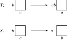
Figure 13: Modular transformations for orbifold models.

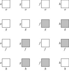
Figure 14: Modular orbits for the $\hbox{\smbm Z}_{2}\times\hbox{\smbm Z}_{2}$ orbifold.

Aside from the identity, that we shall denote by $o$, the $\hbox{\mbm Z}_{2}\times\hbox{\mbm Z}_{2}$ orbifold group contains three other elements acting on the internal $T^{6}=T^{2}\times T^{2}\times T^{2}$ as

$$g:(+,-,-)\,,\qquad f:(-,+,-)\,,\qquad h:(-,-,+)\,,$$ (398)

that give rise to three independent twisted sectors, confined to corresponding fixed tori. The modular transformations of the Jacobi theta-functions in eq. (113) and the corresponding properties of the individual orbifold amplitudes in figure 13 show rather clearly that the sixteen blocks of this $\hbox{\mbm Z}_{2}\times\hbox{\mbm Z}_{2}$ orbifold do not belong to a single modular orbit. For instance, there is no way to generate the $(g,f)$ amplitude from the untwisted ones, and actually the white and grey boxes in figure 14 are associated to two independent orbits, both closed under the action of the modular group. Consequently, one has the freedom to modify the projections on the twisted sectors associating to the disconnected orbit a phase, in this case a pure sign, consistently with the order of the orbifold-group generators [150], and as a result the IIB string on the $\hbox{\mbm Z}_{2}\times\hbox{\mbm Z}_{2}$ orbifold admits the two inequivalent torus amplitudes

$${\cal T} = {\textstyle{1\over 4}}\Biggl{\{}|T_{oo}|^{2}\Lambda_{1}\Lambda_{2}\Lambda_{3}+|T_{og}|^{2}\Lambda_{1}\left|{4\eta^{2}\over\vartheta_{2}^{2}}\right|^{2}$$

$$+|T_{of}|^{2}\Lambda_{2}\left|{4\eta^{2}\over\vartheta_{2}^{2}}\right|^{2}+|T_{oh}|^{2}\Lambda_{3}\left|{4\eta^{2}\over\vartheta_{2}^{2}}\right|^{2}$$

$$+|T_{go}|^{2}\Lambda_{1}\left|{4\eta^{2}\over\vartheta_{4}^{2}}\right|^{2}+|T_{gg}|^{2}\Lambda_{1}\left|{4\eta^{2}\over\vartheta_{3}^{2}}\right|^{2}+|T_{fo}|^{2}\Lambda_{2}\left|{4\eta^{2}\over\vartheta_{4}^{2}}\right|^{2}$$

$$+|T_{ff}|^{2}\Lambda_{2}\left|{4\eta^{2}\over\vartheta_{3}^{2}}\right|^{2}+|T_{ho}|^{2}\Lambda_{3}\left|{4\eta^{2}\over\vartheta_{4}^{2}}\right|^{2}+|T_{hh}|^{2}\Lambda_{3}\left|{4\eta^{2}\over\vartheta_{3}^{2}}\right|^{2}$$

$$+\epsilon\left(|T_{gh}|^{2}+|T_{gf}|^{2}+|T_{fg}|^{2}+|T_{fh}|^{2}+|T_{hg}|^{2}+|T_{hf}|^{2}\right)\left|{8\eta^{3}\over\vartheta_{2}\vartheta_{3}\vartheta_{4}}\right|^{2}\Biggr{\}}\,,$$

where the $\Lambda_{k}$’s are lattice sums for the three internal two-tori and the choices $\epsilon=\mp 1$ identify the models with and without discrete torsion. Here we have expressed the torus amplitude in terms of the 16 quantities $(k=o,g,h,f)$

$$T_{ko} = \tau_{ko}+\tau_{kg}+\tau_{kh}+\tau_{kf}\,,\qquad T_{kg}=\tau_{ko}+\tau_{kg}-\tau_{kh}-\tau_{kf}\,,$$

$$T_{kh} = \tau_{ko}-\tau_{kg}+\tau_{kh}-\tau_{kf}\,,\qquad T_{kf}=\tau_{ko}-\tau_{kg}-\tau_{kh}+\tau_{kf}\,,$$ (400)

where the $16$ $\hbox{\mbm Z}_{2}\times\hbox{\mbm Z}_{2}$ characters $\tau_{kl}$, combinations of products of level-one so(2) characters, are displayed in table 5. The low-energy spectra of the two models are quite different: with discrete torsion, i.e. if $\epsilon=-1$, one has ${\cal N}=2$ supergravity coupled to 52 hyper multiplets and 3 vector multiplets, while without discrete torsion, i.e. if $\epsilon=+1$, one has again ${\cal N}=2$ supergravity, but with 4 hyper multiplets and 51 vector multiplets. These two choices describe orbifold limits of mirror Calabi-Yau manifolds with Hodge numbers (51,3) and (3,51), and, from the conformal field theory viewpoint, the former corresponds to the charge-conjugation modular invariant while the latter corresponds to the diagonal one.

Table 5: Space-time characters for the
supersymmetric $\hbox{\smbm Z}_{2}\times\hbox{\smbm Z}_{2}$ model.

• $\tau_{oo}=V_{2}O_{2}O_{2}O_{2}+O_{2}V_{2}V_{2}V_{2}-S_{2}S_{2}S_{2}S_{2}-C_{2}C_{2}C_{2}C_{2}$

  $\tau_{og}=O_{2}V_{2}O_{2}O_{2}+V_{2}O_{2}V_{2}V_{2}-C_{2}C_{2}S_{2}S_{2}-S_{2}S_{2}C_{2}C_{2}$

  $\tau_{oh}=O_{2}O_{2}O_{2}V_{2}+V_{2}V_{2}V_{2}O_{2}-C_{2}S_{2}S_{2}C_{2}-S_{2}C_{2}C_{2}S_{2}$

  $\tau_{of}=O_{2}O_{2}V_{2}O_{2}+V_{2}V_{2}O_{2}V_{2}-C_{2}S_{2}C_{2}S_{2}-S_{2}C_{2}S_{2}C_{2}$

  $\tau_{go}=V_{2}O_{2}S_{2}C_{2}+O_{2}V_{2}C_{2}S_{2}-S_{2}S_{2}V_{2}O_{2}-C_{2}C_{2}O_{2}V_{2}$

  $\tau_{gg}=O_{2}V_{2}S_{2}C_{2}+V_{2}O_{2}C_{2}S_{2}-S_{2}S_{2}O_{2}V_{2}-C_{2}C_{2}V_{2}O_{2}$

  $\tau_{gh}=O_{2}O_{2}S_{2}S_{2}+V_{2}V_{2}C_{2}C_{2}-C_{2}S_{2}V_{2}V_{2}-S_{2}C_{2}O_{2}O_{2}$

  $\tau_{gf}=O_{2}O_{2}C_{2}C_{2}+V_{2}V_{2}S_{2}S_{2}-S_{2}C_{2}V_{2}V_{2}-C_{2}S_{2}O_{2}O_{2}$

  $\tau_{ho}=V_{2}S_{2}C_{2}O_{2}+O_{2}C_{2}S_{2}V_{2}-C_{2}O_{2}V_{2}C_{2}-S_{2}V_{2}O_{2}S_{2}$

  $\tau_{hg}=O_{2}C_{2}C_{2}O_{2}+V_{2}S_{2}S_{2}V_{2}-C_{2}O_{2}O_{2}S_{2}-S_{2}V_{2}V_{2}C_{2}$

  $\tau_{hh}=O_{2}S_{2}C_{2}V_{2}+V_{2}C_{2}S_{2}O_{2}-S_{2}O_{2}V_{2}S_{2}-C_{2}V_{2}O_{2}C_{2}$

  $\tau_{hf}=O_{2}S_{2}S_{2}O_{2}+V_{2}C_{2}C_{2}V_{2}-C_{2}V_{2}V_{2}S_{2}-S_{2}O_{2}O_{2}C_{2}$

  $\tau_{fo}=V_{2}S_{2}O_{2}C_{2}+O_{2}C_{2}V_{2}S_{2}-S_{2}V_{2}S_{2}O_{2}-C_{2}O_{2}C_{2}V_{2}$

  $\tau_{fg}=O_{2}C_{2}O_{2}C_{2}+V_{2}S_{2}V_{2}S_{2}-C_{2}O_{2}S_{2}O_{2}-S_{2}V_{2}C_{2}V_{2}$

  $\tau_{fh}=O_{2}S_{2}O_{2}S_{2}+V_{2}C_{2}V_{2}C_{2}-C_{2}V_{2}S_{2}V_{2}-S_{2}O_{2}C_{2}O_{2}$

  $\tau_{ff}=O_{2}S_{2}V_{2}C_{2}+V_{2}C_{2}O_{2}S_{2}-C_{2}V_{2}C_{2}O_{2}-S_{2}O_{2}S_{2}V_{2}$

The $\Omega$ projections for the two classes of models can be implemented by the Klein-bottle amplitudes

$${\cal K} = {\textstyle\frac{1}{8}}\Biggl{\{}(P_{1}P_{2}P_{3}+P_{1}W_{2}W_{3}+W_{1}P_{2}W_{3}+W_{1}W_{2}P_{3})T_{oo}$$ (401)

$$+2\times 16\Bigl{[}\epsilon_{1}(P_{1}+\epsilon W_{1})T_{go}+\epsilon_{2}(P_{2}+\epsilon W_{2})T_{fo}$$

$$+\epsilon_{3}(P_{3}+\epsilon W_{3})T_{ho}\Bigr{]}\left(\frac{\eta}{\vartheta_{4}}\right)^{2}\Biggr{\}}\,,$$

where, as usual, $P_{k}$ and $W_{k}$ denote the restrictions of the lattice sums $\Lambda_{k}$ to their momentum and winding sub-lattices. Discrete torsion has a neat effect on $(P_{k}+\epsilon W_{k})$: as anticipated, if $\epsilon=+1$ the massless twisted contributions are diagonal combinations of the $\tau_{kl}$, and appear in the Klein bottle, while if $\epsilon=-1$ they are off-diagonal combinations, and thus do not contribute to it. Consistently with the crosscap constraint of [55, 56, 57], (401) can actually accommodate three additional signs $\epsilon_{k}$ that, however, are not independent, but are to satisfy the constraint

$$\epsilon_{1}\,\epsilon_{2}\,\epsilon_{3}\,=\,\epsilon\,.$$ (402)

One can write this amplitude more compactly as

$${\cal K}={\textstyle\frac{1}{8}}\left[(P_{1}P_{2}P_{3}+{\textstyle\frac{1}{2}}P_{k}W_{l}W_{m})T_{oo}+2\times 16\epsilon_{k}(P_{k}+\epsilon W_{k})T_{ko}\left(\frac{\eta}{\vartheta_{4}}\right)^{2}\right]\,,$$ (403)

where for the sake of brevity we have introduced a convenient shorthand notation, so that summations over repeated indices and symmetrizations over distinct indices are left implicit, with $k$, $l$ and $m$ taking the values $(1,2,3)$. An $S$ transformation then turns this expression into the corresponding transverse-channel amplitude

$$\tilde{\cal K} = \frac{2^{5}}{8}\Biggl{[}\left(v_{1}v_{2}v_{3}W^{e}_{1}W^{e}_{2}W^{e}_{3}+\frac{v_{k}}{2v_{l}v_{m}}W_{k}^{e}P_{l}^{e}P_{m}^{e}\right)T_{oo}$$ (404)

$$+2\epsilon_{k}\,\left(v_{k}W_{k}^{e}+\epsilon\frac{P_{k}^{e}}{v_{k}}\right)\,T_{ok}\left(\frac{2\eta}{\vartheta_{2}}\right)^{2}\Biggr{]}\,,$$

where the superscript $e$ denotes the restriction of the lattice sums to their even terms and the $v_{k}$’s are proportional to the dimensionless volumes of the three internal tori. At the origin of the lattices, the constraint (402) leads to

$$\tilde{\cal K}_{0} = \frac{2^{5}}{8}\Biggl{\{}\left(\sqrt{v_{1}v_{2}v_{3}}+\epsilon_{1}\sqrt{\frac{v_{1}}{v_{2}v_{3}}}+\epsilon_{2}\sqrt{\frac{v_{2}}{v_{1}v_{3}}}+\epsilon_{3}\sqrt{\frac{v_{3}}{v_{1}v_{2}}}\right)^{2}\tau_{oo}$$ (405)

$$+\left(\sqrt{v_{1}v_{2}v_{3}}+\epsilon_{1}\sqrt{\frac{v_{1}}{v_{2}v_{3}}}-\epsilon_{2}\sqrt{\frac{v_{2}}{v_{1}v_{3}}}-\epsilon_{3}\sqrt{\frac{v_{3}}{v_{1}v_{2}}}\right)^{2}\tau_{og}$$

$$+\left(\sqrt{v_{1}v_{2}v_{3}}-\epsilon_{1}\sqrt{\frac{v_{1}}{v_{2}v_{3}}}+\epsilon_{2}\sqrt{\frac{v_{2}}{v_{1}v_{3}}}-\epsilon_{3}\sqrt{\frac{v_{3}}{v_{1}v_{2}}}\right)^{2}\tau_{of}$$

$$+\left(\sqrt{v_{1}v_{2}v_{3}}-\epsilon_{1}\sqrt{\frac{v_{1}}{v_{2}v_{3}}}-\epsilon_{2}\sqrt{\frac{v_{2}}{v_{1}v_{3}}}+\epsilon_{3}\sqrt{\frac{v_{3}}{v_{1}v_{2}}}\right)^{2}\tau_{oh}\Biggr{\}}\,,$$

whose coefficients are as usual perfect squares, that shows clearly how moving from $\epsilon_{k}=1$ to $\epsilon_{k}=-1$ reverses both the tension and the charge of the O$5_{k}$ orientifold plane, thus trading an O$5_{k,+}$ for an O$5_{k,-}$. While manifestly compatible with the usual positivity requirements, this reversal clearly affects the tadpole conditions, that, as in subsection 5.8, require the introduction of antibranes. We are thus facing another, more intricate manifestation of “brane supersymmetry breaking”. In this respect, it should be appreciated that, according to (402), discrete torsion implies the reversal of tension and charge for an odd number of O5 planes. Therefore, the allowed $\epsilon_{k}$’s identify four classes of models. If $\epsilon=+1$, the choice $(\epsilon_{1},\epsilon_{2},\epsilon_{3})=(+,+,+)$ recovers the model discussed in [151, 152], with $48$ chiral multiplets from the closed twisted sectors, while the choice $(+,-,-)$ gives a model with $16$ chiral multiplets and $32$ vector multiplets from the twisted sectors. On the other hand, for $\epsilon=-1$ the two choices $(+,+,-)$ and $(-,-,-)$ yield identical massless twisted spectra, with $48$ chiral multiplets.

In order to describe the open sector, it is convenient to introduce a compact notation, defining

$$\tilde{T}_{kl}^{(\zeta)}=T_{kl}^{\rm NS}-\zeta T_{kl}^{\rm R}\,,\qquad\zeta=\pm 1\,,$$ (406)

where $T_{kl}^{\rm NS}$ and $T_{kl}^{\rm R}$ denote the NS and R parts of the usual supersymmetric $\hbox{\mbm Z}_{2}\times\hbox{\mbm Z}_{2}$ characters. Whereas transverse and direct supersymmetric annulus amplitudes involve the identical sets of characters $\tilde{T}_{kl}^{(+)}$ and ${T}_{kl}^{(+)}$, simply denoted by $T_{kl}$ in the following, in the presence of brane supersymmetry breaking the transverse amplitudes involve the $\tilde{T}_{kl}^{(-)}$, with reversed R-R contributions, that are mapped into new characters by the $S$ modular transformation. As a result, the terms in ${\cal A}$ describing open strings stretched between branes and antibranes contain the new combinations $T^{(-)}_{kl}$, obtained from the $T^{(+)}_{kl}$ interchanging $O_{2}$ with $V_{2}$ and $S_{2}$ with $C_{2}$ in the last three factors, as summarized in table 6.

Table 6: Space-time characters for the
non-supersymmetric $\hbox{\smbm Z}_{2}\times\hbox{\smbm Z}_{2}$ model.

• $\tau^{(-)}_{oo}=O_{2}O_{2}O_{2}O_{2}+V_{2}V_{2}V_{2}V_{2}-C_{2}S_{2}S_{2}S_{2}-S_{2}C_{2}C_{2}C_{2}$

  $\tau^{(-)}_{og}=V_{2}V_{2}O_{2}O_{2}+O_{2}O_{2}V_{2}V_{2}-S_{2}C_{2}S_{2}S_{2}-C_{2}S_{2}C_{2}C_{2}$

  $\tau^{(-)}_{oh}=V_{2}O_{2}O_{2}V_{2}+O_{2}V_{2}V_{2}O_{2}-S_{2}S_{2}S_{2}C_{2}-C_{2}C_{2}C_{2}S_{2}$

  $\tau^{(-)}_{of}=V_{2}O_{2}V_{2}O_{2}+O_{2}V_{2}O_{2}V_{2}-S_{2}S_{2}C_{2}S_{2}-C_{2}C_{2}S_{2}C_{2}$

  $\tau^{(-)}_{go}=O_{2}O_{2}S_{2}C_{2}+V_{2}V_{2}C_{2}S_{2}-C_{2}S_{2}V_{2}O_{2}-S_{2}C_{2}O_{2}V_{2}$

  $\tau^{(-)}_{gg}=V_{2}V_{2}S_{2}C_{2}+O_{2}O_{2}C_{2}S_{2}-C_{2}S_{2}O_{2}V_{2}-S_{2}C_{2}V_{2}O_{2}$

  $\tau^{(-)}_{gh}=V_{2}O_{2}S_{2}S_{2}+O_{2}V_{2}C_{2}C_{2}-S_{2}S_{2}V_{2}V_{2}-C_{2}C_{2}O_{2}O_{2}$

  $\tau^{(-)}_{gf}=V_{2}O_{2}C_{2}C_{2}+O_{2}V_{2}S_{2}S_{2}-C_{2}C_{2}V_{2}V_{2}-S_{2}S_{2}O_{2}O_{2}$

  $\tau^{(-)}_{ho}=O_{2}S_{2}C_{2}O_{2}+V_{2}C_{2}S_{2}V_{2}-S_{2}O_{2}V_{2}C_{2}-C_{2}V_{2}O_{2}S_{2}$

  $\tau^{(-)}_{hg}=V_{2}C_{2}C_{2}O_{2}+O_{2}S_{2}S_{2}V_{2}-S_{2}O_{2}O_{2}S_{2}-C_{2}V_{2}V_{2}C_{2}$

  $\tau^{(-)}_{hh}=V_{2}S_{2}C_{2}V_{2}+O_{2}C_{2}S_{2}O_{2}-C_{2}O_{2}V_{2}S_{2}-S_{2}V_{2}O_{2}C_{2}$

  $\tau^{(-)}_{hf}=V_{2}S_{2}S_{2}O_{2}+O_{2}C_{2}C_{2}V_{2}-S_{2}V_{2}V_{2}S_{2}-C_{2}O_{2}O_{2}C_{2}$

  $\tau^{(-)}_{fo}=O_{2}S_{2}O_{2}C_{2}+V_{2}C_{2}V_{2}S_{2}-C_{2}V_{2}S_{2}O_{2}-S_{2}O_{2}C_{2}V_{2}$

  $\tau^{(-)}_{fg}=V_{2}C_{2}O_{2}C_{2}+O_{2}S_{2}V_{2}S_{2}-S_{2}O_{2}S_{2}O_{2}-C_{2}V_{2}C_{2}V_{2}$

  $\tau^{(-)}_{fh}=V_{2}S_{2}O_{2}S_{2}+O_{2}C_{2}V_{2}C_{2}-S_{2}V_{2}S_{2}V_{2}-C_{2}O_{2}C_{2}O_{2}$

  $\tau^{(-)}_{ff}=V_{2}S_{2}V_{2}C_{2}+O_{2}C_{2}O_{2}S_{2}-S_{2}V_{2}C_{2}O_{2}-C_{2}O_{2}S_{2}V_{2}$

The transverse-channel annulus amplitude is

$$\tilde{{\cal A}} = \frac{2^{-5}}{8}\Biggl{\{}\left(N_{o}^{2}v_{1}v_{2}v_{3}W_{1}W_{2}W_{3}+\frac{D_{k;o}^{2}v_{k}}{2v_{l}v_{m}}W_{k}P_{l}P_{m}\right)T_{oo}$$ (407)

$$+4\left[(N_{k}^{2}+D^{2}_{k;k})v_{k}W_{k}+D^{2}_{l\neq k;k}\frac{P_{k}}{v_{k}}\right]T_{ko}\left(\frac{2\eta}{\vartheta_{4}}\right)^{2}$$

$$+2N_{o}D_{k;o}v_{k}W_{k}{\tilde{T}}_{ok}^{(\epsilon_{k})}\left(\frac{2\eta}{\vartheta_{2}}\right)^{2}+2N_{k}D_{k;k}v_{k}W_{k}{\tilde{T}}_{kk}^{(\epsilon_{k})}\left(\frac{2\eta}{\vartheta_{3}}\right)^{2}$$

$$+4N_{l}D_{k\neq l;l}{\tilde{T}}_{lk}^{(\epsilon_{k})}\frac{8\eta^{3}}{\vartheta_{2}\vartheta_{3}\vartheta_{4}}+D_{k;o}D_{l;o}\frac{P_{m}}{v_{m}}{\tilde{T}}_{om}^{(\epsilon_{k}\epsilon_{l})}\left(\frac{2\eta}{\vartheta_{2}}\right)^{2}$$

$$+D_{k;m}D_{l;m}\frac{P_{m}}{v_{m}}{\tilde{T}}_{mm}^{(\epsilon_{k}\epsilon_{l})}\left(\frac{2\eta}{\vartheta_{3}}\right)^{2}+4D_{k;k}D_{l;k}{\tilde{T}}_{km}^{(\epsilon_{k}\epsilon_{l})}\frac{8\eta^{3}}{\vartheta_{2}\vartheta_{3}\vartheta_{4}}\Biggr{\}}\,,$$

where $N_{o}$, $D_{g;o}$, $D_{f;o}$ and $D_{h;o}$ count the numbers of D9 branes and of the three sets of D5 or $\overline{\rm D}5$ branes wrapped around the first, second and third torus, denoted for brevity $5_{1,2,3}$ or $\bar{5}_{1,2,3}$ in the following. In a similar fashion, $N_{k}$, $D_{g;k}$, $D_{f;k}$ and $D_{h;k}$ $(k=g,f,h)$ parametrize the breakings induced by the three orbifold operations $g$, $f$ and $h$. Notice that, as in subsection 5.8, the R-R portions of all terms describing brane-antibrane exchanges have reversed signs. The untwisted terms at the origin of the lattice sums rearrange themselves into perfect squares, so that

$$\tilde{\cal A}_{0}=$$ (408)

$$\frac{2^{-5}}{8}\Biggl{\{}\ \left(N_{o}\sqrt{v_{1}v_{2}v_{3}}+D_{g;o}\sqrt{\frac{v_{1}}{v_{2}v_{3}}}+D_{f;o}\sqrt{\frac{v_{2}}{v_{1}v_{3}}}+D_{h;o}\sqrt{\frac{v_{3}}{v_{1}v_{2}}}\right)^{2}\tau^{\rm NS}_{oo}$$

$$-\left(N_{o}\sqrt{v_{1}v_{2}v_{3}}+\epsilon_{1}D_{g;o}\sqrt{\frac{v_{1}}{v_{2}v_{3}}}+\epsilon_{2}D_{f;o}\sqrt{\frac{v_{2}}{v_{1}v_{3}}}+\epsilon_{3}D_{h,o}\sqrt{\frac{v_{3}}{v_{1}v_{2}}}\right)^{2}\tau^{\rm R}_{oo}$$

$$+\left(N_{o}\sqrt{v_{1}v_{2}v_{3}}+D_{g;o}\sqrt{\frac{v_{1}}{v_{2}v_{3}}}-D_{f;o}\sqrt{\frac{v_{2}}{v_{1}v_{3}}}-D_{h;o}\sqrt{\frac{v_{3}}{v_{1}v_{2}}}\right)^{2}\tau^{\rm NS}_{og}$$

$$-\left(N_{o}\sqrt{v_{1}v_{2}v_{3}}+\epsilon_{1}D_{g;o}\sqrt{\frac{v_{1}}{v_{2}v_{3}}}-\epsilon_{2}D_{f;o}\sqrt{\frac{v_{2}}{v_{1}v_{3}}}-\epsilon_{3}D_{h;o}\sqrt{\frac{v_{3}}{v_{1}v_{2}}}\right)^{2}\tau^{\rm R}_{og}$$

$$+\left(N_{o}\sqrt{v_{1}v_{2}v_{3}}-D_{g;o}\sqrt{\frac{v_{1}}{v_{2}v_{3}}}+D_{f;o}\sqrt{\frac{v_{2}}{v_{1}v_{3}}}-D_{h;o}\sqrt{\frac{v_{3}}{v_{1}v_{2}}}\right)^{2}\tau^{\rm NS}_{of}$$

$$-\left(N_{o}\sqrt{v_{1}v_{2}v_{3}}-\epsilon_{1}D_{g;o}\sqrt{\frac{v_{1}}{v_{2}v_{3}}}+\epsilon_{2}D_{f;o}\sqrt{\frac{v_{2}}{v_{1}v_{3}}}-\epsilon_{3}D_{h;o}\sqrt{\frac{v_{3}}{v_{1}v_{2}}}\right)^{2}\tau^{\rm R}_{of}$$

$$+\left(N_{o}\sqrt{v_{1}v_{2}v_{3}}-D_{g;o}\sqrt{\frac{v_{1}}{v_{2}v_{3}}}-D_{f;o}\sqrt{\frac{v_{2}}{v_{1}v_{3}}}+D_{h;o}\sqrt{\frac{v_{3}}{v_{1}v_{2}}}\right)^{2}\tau^{\rm NS}_{oh}$$

$$-\left(N_{o}\sqrt{v_{1}v_{2}v_{3}}-\epsilon_{1}D_{g;o}\sqrt{\frac{v_{1}}{v_{2}v_{3}}}-\epsilon_{2}D_{f;o}\sqrt{\frac{v_{2}}{v_{1}v_{3}}}+\epsilon_{3}D_{h;o}\sqrt{\frac{v_{3}}{v_{1}v_{2}}}\right)^{2}\tau^{\rm R}_{oh}\ \Biggr{\}}\,.$$

The twisted tadpoles reflect rather neatly the geometry of the brane configuration. As usual, the reflection coefficients are sums of squares associated to the various fixed tori, and each square contains the projections for the branes that are present, with factors $\sqrt{v_{i}}$ if they are wrapped around them and $1/\sqrt{v_{i}}$ if they are localized on them. The relative coefficients of these terms, also directly linked to the brane geometry, are given by

$$\sqrt{\frac{\rm\#\ of\ fixed\ tori}{\rm\#\ of\ occupied\ fixed\ tori}}\,.$$ (409)

Thus, for a given twisted sector, the numerator counts the fixed tori, while the denominator counts the fixed tori where branes are actually present. Moreover, the R portions of the characters describing brane-antibrane exchanges have reversed signs even in these twisted contributions, as expected. For instance, in the $g$-twisted sector of the $(+,+,-)$ model, that contains $\overline{\rm D}5_{3}$ branes, the reflection coefficients for the massless modes in $\tau_{gh}$ are

$$\frac{2^{-5}}{8}\Biggl{[}\left(N_{g}\sqrt{v_{1}}-4D_{g;g}\sqrt{v_{1}}-2D_{f;g}\frac{1}{\sqrt{v_{1}}}+2D_{h;g}\frac{1}{\sqrt{v_{1}}}\right)^{2}+9N_{g}^{2}v_{1}$$

$$+3\left(N_{g}\sqrt{v_{1}}-2D_{f;g}\frac{1}{\sqrt{v_{1}}}\right)^{2}+3\left(N_{g}\sqrt{v_{1}}+2D_{h;g}\frac{1}{\sqrt{v_{1}}}\right)^{2}\Biggr{]}$$ (410)

for the NS-NS portion, and

$$\frac{2^{-5}}{8}\Biggl{[}\left(N_{g}\sqrt{v_{1}}-4D_{g;g}\sqrt{v_{1}}-2D_{f;g}\frac{1}{\sqrt{v_{1}}}-2D_{h;g}\frac{1}{\sqrt{v_{1}}}\right)^{2}+9N_{g}^{2}v_{1}$$

$$+3\left(N_{g}\sqrt{v_{1}}-2D_{f;g}\frac{1}{\sqrt{v_{1}}}\right)^{2}+3\left(N_{g}\sqrt{v_{1}}-2D_{h;g}\frac{1}{\sqrt{v_{1}}}\right)^{2}\Biggr{]}$$ (411)

for the R-R portion. According to (409), the coefficient of $N_{g}$ is $\sqrt{v_{1}}$, since the D9’s are wrapped around all fixed tori, the coefficient of $D_{g;g}$ is $4\sqrt{v_{1}}$, since the D$5_{1}$’s are only wrapped around one fixed torus, while the coefficients of $D_{f;g}$ and $D_{h;g}$ are $2/\sqrt{v_{1}}$, since the D$5_{2}$’s and $\overline{\rm D}5_{3}$’s are confined to four of the fixed tori. Finally, out of the 16 $g$-fixed tori, one sees all the branes, three see only the D9’s and the D$5_{2}$’s, three see only the D9’s and the $\overline{\rm D}5_{3}$’s and, finally, nine see only the D9’s.

The direct-channel annulus amplitude is then

$${\cal A} = {\textstyle\frac{1}{8}}\Biggl{\{}\left(N_{o}^{2}P_{1}P_{2}P_{3}+\frac{D_{k;o}^{2}}{2}P_{k}W_{l}W_{m}\right)T_{oo}$$

$$+\left[(N_{k}^{2}+D^{2}_{k;k})P_{k}+D^{2}_{l\neq k;k}W_{k}\right]T_{ok}\left(\frac{2\eta}{\vartheta_{2}}\right)^{2}$$

$$+2N_{o}D_{k;o}P_{k}T_{ko}^{(\epsilon_{k})}\left(\frac{\eta}{\vartheta_{4}}\right)^{2}-2N_{k}D_{k;k}P_{k}T_{kk}^{(\epsilon_{k})}\left(\frac{\eta}{\vartheta_{3}}\right)^{2}$$

$$+2i(-1)^{k+l}N_{l}D_{k\neq l;l}T_{kl}^{(\epsilon_{k})}\frac{2\eta^{3}}{\vartheta_{2}\vartheta_{3}\vartheta_{4}}+D_{k;o}D_{l;o}W_{m}T_{mo}^{(\epsilon_{k}\epsilon_{l})}\left(\frac{\eta}{\vartheta_{4}}\right)^{2}$$

$$-D_{k;m}D_{l;m}W_{m}T_{mm}^{(\epsilon_{k}\epsilon_{l})}\left(\frac{\eta}{\vartheta_{3}}\right)^{2}+2i(-1)^{m+k}D_{k;k}D_{l;k}T_{mk}^{(\epsilon_{k}\epsilon_{l})}\frac{2\eta^{3}}{\vartheta_{2}\vartheta_{3}\vartheta_{4}}\Biggr{\}}\,,$$

where in the signs $(-1)^{k+l}$ and $(-1)^{m+k}$ the integers $k,l,m$ take the values $1,2,3$ for the $g$, $f$, and $h$ generators. $\tilde{\cal K}$ and $\tilde{\cal A}$ determine by standard methods the transverse-channel Möbius amplitude

$$\tilde{{\cal M}} = -{\textstyle\frac{1}{4}}\Biggl{\{}N_{o}v_{1}v_{2}v_{3}W^{e}_{1}W^{e}_{2}W^{e}_{3}\hat{T}_{oo}+N_{o}v_{k}W^{e}_{k}\epsilon_{k}\hat{T}_{ok}\left(\frac{2\hat{\eta}}{\hat{\vartheta_{2}}}\right)^{2}$$ (413)

$$+\frac{v_{k}}{2v_{l}v_{m}}D_{k;o}W^{e}_{k}P^{e}_{l}P^{e}_{m}\epsilon_{k}\hat{\tilde{T}}{}_{oo}^{(\epsilon_{k})}$$

$$+\left(D_{l;o}\epsilon_{k}\frac{P^{e}_{m}}{v_{m}}\hat{\tilde{T}}{}_{om}^{(\epsilon_{l})}+D_{k;o}v_{k}W^{e}_{k}\hat{\tilde{T}}{}_{ok}^{(\epsilon_{k})}\right)\left(\frac{2\hat{\eta}}{\hat{\vartheta_{2}}}\right)^{2}\Biggr{\}}\,,$$

and after a $P$ transformation,

$${\cal M} = -{\textstyle\frac{1}{8}}\Biggl{\{}N_{o}P_{1}P_{2}P_{3}\hat{T}_{oo}-N_{o}P_{k}\epsilon_{k}\hat{T}_{ok}\left(\frac{2\hat{\eta}}{\hat{\vartheta_{2}}}\right)^{2}+{\textstyle\frac{1}{2}}D_{k;o}P_{k}W_{l}W_{m}\epsilon_{k}\hat{\tilde{T}}{}_{oo}^{(\epsilon_{k})}$$ (414)

$$-\left(D_{l;o}\epsilon_{k}W_{m}\hat{\tilde{T}}{}_{om}^{(\epsilon_{l})}+D_{k;o}P_{k}\hat{\tilde{T}}{}_{ok}^{(\epsilon_{k})}\right)\left(\frac{2\hat{\eta}}{\hat{\vartheta_{2}}}\right)^{2}\Biggr{\}}\,.$$

From the transverse amplitudes one can finally read the R-R tadpole conditions

$$N_{o}=32\,,\qquad N_{g}=N_{f}=N_{h}=0\,,$$ (415)

$$D_{k;o}=32\,,\qquad D_{k;g}=D_{k;f}=D_{k;h}=0\,.$$

In the presence of discrete torsion the NS-NS tadpole conditions are incompatible with the R-R ones, and, as in all models featuring brane supersymmetry breaking, a dilaton tadpole and a potential for geometric moduli are generated.

We can now conclude with a brief discussion of the massless spectra. The models where only one $\epsilon_{k}$ is negative have discrete torsion and contain one $\overline{\rm D}5$. For the D9 and the two sets of D5 branes, the gauge groups are ${\rm U}(8)\times{\rm U}(8)$, with ${\cal N}=1$ supersymmetry, while for the $\overline{\rm D}5$ branes the gauge group is ${\rm USp}(8)^{4}$, with ${\cal N}=0$. Moreover, the 95 and $5_{k}5_{l}$ strings are supersymmetric, while the $9\bar{5}$ and $5_{k}\bar{5}$ strings are not. Let us discuss in some detail the case $(\epsilon_{1},\epsilon_{2},\epsilon_{3})=(+,+,-)$, that contains $\overline{\rm D}5$ branes wrapped around the third torus. To this end, let us parametrize the charges as

$$N_{o} =o+g+\bar{o}+\bar{g}\,,\hskip 68.28644pt N_{g}=i(o+g-\bar{o}-\bar{g})\,,$$

$$N_{f} =i(o-g-\bar{o}+\bar{g})\,, N_{h}=o-g+\bar{o}-\bar{g}\,,$$

$$D_{g;o} =o_{1}+g_{1}+\bar{o}_{1}+\bar{g}_{1}\,, D_{g;g}=i(o_{1}+g_{1}-\bar{o}_{1}-\bar{g}_{1})\,,$$

$$D_{g;f} =o_{1}-g_{1}+\bar{o}_{1}-\bar{g}_{1}\,, D_{g;h}=-i(o_{1}-g_{1}-\bar{o}_{1}+\bar{g}_{1})\,,$$

$$D_{f;o} =o_{2}+g_{2}+\bar{o}_{2}+\bar{g}_{2}\,, D_{f;g}=o_{2}-g_{2}+\bar{o}_{2}-\bar{g}_{2}\,,$$

$$D_{f;f} =i(o_{2}+g_{2}-\bar{o}_{2}-\bar{g}_{2})\,, D_{f;h}=i(o_{2}-g_{2}-\bar{o}_{2}+\bar{g}_{2})\,,$$

$$D_{h;o} =a+b+c+d\,, D_{h;g}=a+b-c-d\,,$$

$$D_{h;f} =a-b+c-d\,, D_{h;h}=a-b-c+d\,,$$ (416)

and extract the massless spectrum from the amplitudes at the origin of the lattices. As anticipated, the $99$, $5_{1}5_{1}$ and $5_{2}5_{2}$ sectors have ${\cal N}=1$ supersymmetry, with ${\rm U}(8)\times{\rm U}(8)$ gauge groups and chiral multiplets in the representations $(8,8)$, $(8,\bar{8})$, $(28,1)$, $(1,28)$ and their conjugates. Moreover, as expected, the $95_{1}$, $95_{2}$ and $5_{1}5_{2}$ strings are also supersymmetric, and contain chiral multiplets in the representations

$$95_{1}:\ (8,1;1,\bar{8})\,,\ \ (1,8;\bar{8},1)\,,\ \ (\bar{8},1;8,1)\,,\ \ (1,\bar{8};1,8)\,,$$

$$95_{2}:\ (8,1;1,\bar{8})\,,\ \ (1,\bar{8};\bar{8},1)\,,\ \ (\bar{8},1;8,1)\,,\ \ (1,8;1,8)\,,$$

$$5_{1}5_{2}:\ (8,1;8,1)\,,\ \ (1,8;\bar{8},1)\,,\ \ (\bar{8},1;1,8)\,,\ \ (1,\bar{8};1,\bar{8})\,.$$

On the other hand, the strings that end on the antibrane yield non-supersymmetric spectra, even if the annulus contains supersymmetric characters, since bosons and fermions are treated differently by ${\cal M}$. Thus, the $\bar{5}_{3}\bar{5}_{3}$ excitations have a ${\rm USp}(8)^{4}$ gauge group, with Weyl spinors in the $(28,1,1,1)$ and in three additional permutations, and chiral multiplets in the $(8,8,1,1)$ and in five additional permutations. Finally, the strings stretching between a brane and an antibrane have non-supersymmetric spectra, with Weyl spinors and complex scalars in the representations

$$9\bar{5}_{3} {\rm spinors\ :} \ (\bar{8},1;8,1,1,1)\,,\ \ (1,\bar{8};1,8,1,1)\,,$$

$$\ (1,8;1,1,8,1)\,,\ \ (8,1;1,1,1,8)\,,$$

$${\rm scalars\ :} \ (\bar{8},1;1,8,1,1)\,,\ \ (1,\bar{8};8,1,1,1)\,,$$

$$\ (1,8;1,1,1,8)\,,\ \ (8,1;1,1,8,1)\,,$$

$$5_{1}\bar{5}_{3} {\rm\ spinors\ :} \ (\bar{8},1;1,1,8,1)\,,\ \ (1,\bar{8};1,1,1,8)\,,$$

$$\ (1,8;1,8,1,1)\,,\ \ (8,1;8,1,1,1)\,,$$

$${\rm scalars\ :} \ (\bar{8},1;1,1,1,8)\,,\ \ (1,\bar{8};1,1,8,1)\,,$$

$$\ (1,8;8,1,1,1)\,,\ \ (8,1;1,8,1,1)\,,$$

$$5_{2}\bar{5}_{3} {\rm\ spinors\ :} \ (8,1;8,1,1,1)\,,\ \ (1,\bar{8};1,1,1,8)\,,$$

$$\ (1,8;1,1,8,1)\,,\ \ (\bar{8},1;1,8,1,1)\,,$$

$${\rm scalars\ :} \ (\bar{8},1;1,1,1,8)\,,\ \ (1,\bar{8};1,8,1,1)\,,$$

$$\ (1,8;8,1,1,1)\,,\ \ (8,1;1,1,8,1)\,.$$

The choice $(\epsilon_{1},\epsilon_{2},\epsilon_{3})=(-,-,-)$ corresponds again to a model with discrete torsion. In this case, however, there are D9 branes and three sets of $\overline{\rm D}5$ branes, while the charges are to be parametrized as

$$N_{o} =a+b+c+d\,,\hskip 68.28644pt N_{g}=a+b-c-d\,,$$

$$N_{f} =a-b+c-d\,, N_{h}=a-b-c+d\,,$$

$$D_{g;o} =o_{1}+g_{1}+\bar{o}_{1}+\bar{g}_{1}\,, D_{g;g}=o_{1}-g_{1}+\bar{o}_{1}-\bar{g}_{1}\,,$$

$$D_{g;f} =i(o_{1}+g_{1}-\bar{o}_{1}-\bar{g}_{1})\,, D_{g;h}=i(o_{1}-g_{1}-\bar{o}_{1}+\bar{g}_{1})\,,$$

$$D_{f;o} =o_{2}+g_{2}+\bar{o}_{2}+\bar{g}_{2}\,, D_{f;g}=i(o_{2}+g_{2}-\bar{o}_{2}-\bar{g}_{2})\,,$$

$$D_{f;f} =o_{2}-g_{2}+\bar{o}_{2}-\bar{g}_{2}\,, D_{f;h}=-i(o_{2}-g_{2}-\bar{o}_{2}+\bar{g}_{2})\,,$$

$$D_{h;o} =o_{3}+g_{3}+\bar{o}_{3}+\bar{g}_{3}\,, D_{h;g}=i(o_{3}+g_{3}-\bar{o}_{3}-\bar{g}_{3})\,,$$

$$D_{h;f} =i(o_{3}-g_{3}-\bar{o}_{3}+\bar{g}_{3})\,, D_{h;h}=o_{3}-g_{3}+\bar{o}_{3}-\bar{g}_{3}\,.$$ (417)

The D9 branes have ${\cal N}=1$ supersymmetry, but now with gauge group ${\rm SO}(8)^{4}$ and chiral multiplets in the $(8,8,1,1)$ and five permutations. Moreover, each antibrane gives a non-supersymmetric spectrum, with gauge group ${\rm U}(8)\times{\rm U}(8)$, chiral multiplets in the $(8,8)$, $(8,\bar{8})$ and in their conjugates, spinors in the $(28,1)$, $(\overline{28},1)$, $(1,28)$, $(1,\overline{28})$ and complex scalars in the $(36,1)$, $(\overline{36},1)$, $(1,36)$, $(1,\overline{36})$. We would like to stress that in this case the would-be gauginos are massless, since the Möbius amplitude does not affect the adjoint representations of unitary groups. Finally, the $\bar{5}_{k}\bar{5}_{l}$ sectors give chiral multiplets in the representations

$$\bar{5}_{1}\bar{5}_{2}:\ \ (8,1;8,1)\ ,\ \ (\bar{8},1;1,8)\ ,\ \ (1,8;\bar{8},1)\ ,\ \ (1,\bar{8};1,\bar{8})\ ,$$

$$\bar{5}_{1}\bar{5}_{3}:\ \ (8,1;\bar{8},1)\ ,\ \ (\bar{8},1;1,\bar{8})\ ,\ \ (1,8;1,8)\ ,\ \ (1,\bar{8};8,1)\ ,$$

$$\bar{5}_{2}\bar{5}_{3}:\ \ (8,1;\bar{8},1)\ ,\ \ (\bar{8},1;1,8)\ ,\ \ (1,8;1,\bar{8})\ ,\ \ (1,\bar{8};8,1)\ ,$$

while the non-supersymmetric $9\bar{5}_{k}$ sectors give Weyl spinors and complex scalars in the representations

$$9\bar{5}_{1} {\it\ {\rm spinors}\ :} \ (8,1,1,1;8,1)\,,\ \ (1,8,1,1;\bar{8},1)\,,$$

$$\ (1,1,8,1;1,8)\,,\ \ (1,1,1,8;1,\bar{8})\,,$$

$${\it\ {\rm scalars}\ :} \ (8,1,1,1;1,8)\,,\ \ (1,8,1,1;1,\bar{8})\,,$$

$$\ (1,1,8,1;8,1)\,,\ \ (1,1,1,8;\bar{8},1)\,,$$

$$9\bar{5}_{2} {\it\ {\rm spinors}\ :} \ (8,1,1,1;8,1)\,,\ \ (1,8,1,1;1,8)\,,$$

$$\ (1,1,8,1;\bar{8},1)\,,\ \ (1,1,1,8;1,\bar{8})\,,$$

$${\it\ {\rm scalars}\ :} \ (8,1,1,1;1,8)\,,\ \ (1,8,1,1;8,1)\,,$$

$$\ (1,1,8,1;1,\bar{8})\,,\ \ (1,1,1,8;\bar{8},1)\,,$$

$$9\bar{5}_{3} {\it\ {\rm spinors}\ :} \ (8,1,1,1;\bar{8},1)\,,\ \ (1,8,1,1;1,\bar{8})\,,$$

$$\ (1,1,8,1;1,8)\,,\ \ (1,1,1,8;8,1)\,,$$

$${\it\ {\rm scalars}\ :} \ (8,1,1,1;1,\bar{8})\,,\ \ (1,8,1,1;\bar{8},1)\,,$$

$$\ (1,1,8,1;8,1)\,,\ \ (1,1,1,8;1,8)\,.$$

All chiral spectra thus obtained are free of non-Abelian anomalies.

On the other hand, the models without discrete torsion are not chiral. The choice $(\epsilon_{1},\epsilon_{2},\epsilon_{3})=(+,+,+)$, discussed in [151] and worked out in detail in [152], leads to a gauge group ${\rm USp}(16)^{4}$. Another model, without discrete torsion but with two $\overline{\rm D}5$ branes, can be obtained if two of the $\epsilon_{k}$’s are negative. The D9 and D5 branes give orthogonal gauge groups with ${\cal N}=1$ supersymmetry, while the two $\overline{\rm D}5$ branes give symplectic gauge groups with broken supersymmetry. For instance, with the choice $(+,-,-)$

$${\cal A}_{0} = {\textstyle\frac{1}{8}}\biggl{\{}(N_{o}^{2}+D^{2}_{g;o}+D^{2}_{f;o}+D^{2}_{h;o})T_{oo}$$

$$+2N_{o}D_{g;o}T_{go}+2N_{o}D_{f;o}T^{(-)}_{fo}+2N_{o}D_{h;o}T^{(-)}_{ho}$$

$$+2D_{g;o}D_{f;o}T^{(-)}_{ho}+2D_{g;o}D_{h;o}T^{(-)}_{fo}+2D_{f;o}D_{h;o}T_{go}\biggr{\}}\,,$$

$${\cal M}_{0} = -{\textstyle\frac{1}{4}}\biggl{\{}(N_{o}+D_{g;o})(\tau_{oo}-\tau_{og}+\tau_{of}+\tau_{oh})$$ (418)

$$-(D_{f;o}+D_{h;o})(\tau^{{\rm NS}}_{oo}-\tau^{{\rm NS}}_{og}+\tau^{{\rm NS}}_{of}+\tau^{{\rm NS}}_{oh})$$

$$-(D_{f;o}+D_{h;o})(\tau^{{\rm R}}_{oo}-\tau^{{\rm R}}_{og}+\tau^{{\rm R}}_{of}+\tau^{{\rm R}}_{oh})\biggr{\}}\,,$$

where no breaking terms are present. After a suitable rescaling of the charge multiplicities, the $\overline{\rm D}5_{2}$ and the $\overline{\rm D}5_{3}$ branes give non-supersymmetric spectra, with ${\rm USp}(16)$ gauge groups, spinors in the 136 and in three copies of the 120 and scalars in the 120 and in two copies of the 136. The 99 and $5_{1}5_{1}$ sectors have ${\cal N}=1$ supersymmetry, ${\rm SO}(16)$ gauge groups and chiral multiplets in the 136 and in two copies of the 120. Finally, there are two chiral multiplets in the $(16,16)$ arising from the $95_{1}$ and $\bar{5}_{2}\bar{5}_{3}$ sectors and complex scalars and Weyl spinors in bi-fundamental representations arising from the $9\bar{5}_{2}$, $9\bar{5}_{3}$, $5_{1}\bar{5}_{2}$ and $5_{1}\bar{5}_{3}$ sectors. More details can be found in [74].

5.11 Magnetic deformations and supersymmetry

Homogeneous magnetic fields provide an interesting example of a non-trivial deformation compatible with two-dimensional conformal invariance. The study of their effect on open strings is relatively simple [104, 105], for they interact only with the string ends, affecting the world-sheet dynamics via boundary terms. They also provide an interesting way to break supersymmetry in open string models [80, 81, 82], an option extensively investigated in [153].

Let us begin by considering the bosonic string in the presence of a uniform magnetic field, that can be described by the vector potential

$$A_{\mu}=-{\textstyle\frac{1}{2}}F_{\mu\nu}X^{\nu}\,.$$ (419)

The variational principle for the world-sheet action

$$S = -\frac{1}{4\pi\alpha^{\prime}}\,\int d\tau\int_{0}^{\pi}d\sigma\partial_{\alpha}X\cdot\partial^{\alpha}X$$ (420)

$$-\left.q_{\rm L}\int d\tau A_{\mu}\partial_{\tau}X^{\mu}\right|_{\sigma=0}-\left.q_{\rm R}\int d\tau A_{\mu}\partial_{\tau}X^{\mu}\right|_{\sigma=\pi}\,,$$

here written in the conformal gauge for a strip of width $\pi$, yields the wave equations

$$\left({\partial^{2}\over\partial\tau^{2}}-{\partial^{2}\over\partial\sigma^{2}}\right)X^{\mu}=0\,,$$ (421)

together with the boundary conditions

$${1\over 2\pi\alpha^{\prime}}\,\partial_{\sigma}X^{\mu}-q_{\rm L}F^{\mu}{}_{\nu}\,\partial_{\tau}X^{\nu} = 0\,,$$

$${1\over 2\pi\alpha^{\prime}}\,\partial_{\sigma}X^{\mu}+q_{\rm R}F^{\mu}{}_{\nu}\,\partial_{\tau}X^{\nu} = 0\,,$$ (422)

for $\sigma=0,\pi$, that interpolate between the Neumann and Dirichlet cases.

Eq. (422) admits an alternative geometric interpretation in terms of rotated branes [86]. To be specific, let us consider a magnetic field $F_{12}=H$ in a plane $(X^{1},X^{2})$ and perform a T-duality along the $X^{2}$ direction, so that $\partial_{\alpha}X^{2}=\epsilon_{\alpha\beta}\,\partial^{\beta}Y^{2}$ links $X^{2}$ to the dual coordinate $Y^{2}$. The boundary conditions then become standard Neumann and Dirichlet ones

$$\partial_{\sigma}\left(X^{1}-2\pi\alpha^{\prime}q_{\rm L}H\,Y^{2}\right) = 0\,,$$

$$\partial_{\tau}\left(Y^{2}+2\pi\alpha^{\prime}q_{\rm R}H\,X^{1}\right) = 0\,,$$ (423)

that indeed identify branes rotated by an angle

$$\theta_{{\rm L,R}}=-\tan^{-1}(2\pi\alpha^{\prime}q_{{\rm L,R}}H)\,.$$ (424)

It is now convenient to introduce the complex coordinates

$$Z={\textstyle{1\over\sqrt{2}}}(X^{1}+iX^{2})\,,\qquad\bar{Z}={\textstyle{1\over\sqrt{2}}}(X^{1}-iX^{2})\,,$$ (425)

so that the action becomes

$$S = {1\over 2\pi\alpha^{\prime}}\int d\tau\int_{0}^{\pi}d\sigma\,\partial_{\alpha}\bar{Z}\partial^{\alpha}Z$$ (426)

$$+iq_{\rm L}H\left.\int d\tau\bar{Z}\partial_{\tau}Z\right|_{\sigma=0}+iq_{\rm R}H\left.\int d\tau\bar{Z}\partial_{\tau}Z\right|_{\sigma=\pi}\,,$$

while the boundary conditions (422) reduce to

$$\partial_{\sigma}Z+i\alpha\,\partial_{\tau}Z = 0\,,$$

$$\partial_{\sigma}Z-i\beta\,\partial_{\tau}Z = 0\,,$$ (427)

with

$$\alpha=2\pi\alpha^{\prime}q_{\rm L}H\,,\qquad\beta=2\pi\alpha^{\prime}q_{\rm R}H\,.$$ (428)

The solution of the wave equation with these boundary conditions depends on the total charge $Q=q_{\rm L}+q_{\rm R}$ of the open string. If $Q$ is different from zero, the frequencies of the oscillator modes are shifted by [105]

$$\zeta={1\over\pi}(\gamma+\gamma^{\prime})\,,\qquad{\rm with}\qquad\gamma=\tan^{-1}(\alpha)\,,\quad\gamma^{\prime}=\tan^{-1}(\beta)\,,$$ (429)

and the mode expansion becomes

$$Z(\tau,\sigma)=z+i\sqrt{2\alpha^{\prime}}\left[\sum_{n=1}^{\infty}a_{n}\psi_{n}(\tau,\sigma)-\sum_{m=0}^{\infty}b^{\dagger}_{m}\psi_{-m}(\tau,\sigma)\right]\,,$$ (430)

with

$$\psi_{n}(\tau,\sigma)=\frac{1}{\sqrt{|n-\zeta|}}\,\cos\left[(n-\zeta)\sigma+\gamma\right]\,e^{-i(n-\zeta)\tau}\,.$$ (431)

The momentum canonically conjugate to $Z$ is now

$$\bar{\Pi}(\tau,\sigma)=\frac{1}{2\pi\alpha^{\prime}}\left\{\partial_{\tau}Z(\tau,\sigma)-iZ(\tau,\sigma)\left[\alpha\delta(\sigma)+\beta\delta(\pi-\sigma)\right]\right\}\,,$$ (432)

and the usual commutation relations imply that $a_{m}$ and $b^{\dagger}_{m}$ are independent Fourier coefficients, while the zero modes do not commute

$$[z,\bar{z}]=\frac{2\pi\alpha^{\prime}}{\alpha+\beta}\,,$$ (433)

so that their contribution to the Hamiltonian results in the familiar spectrum of Landau levels.

The solution is quite different for the “dipole” strings, with $\beta=-\alpha$, for which $Q=0$. In this case, the oscillator frequencies are no more shifted, while the boundary conditions allow for the presence of new zero modes, so that one can write [105]

$$Z(\tau,\sigma) = \frac{z+\bar{p}\left[\tau-i\alpha(\sigma-\frac{1}{2}\pi)\right]}{\sqrt{1+\alpha^{2}}}$$ (434)

$$+i\sqrt{2\alpha^{\prime}}\sum_{n=1}^{\infty}\left[a_{n}\psi_{n}(\tau,\sigma)-b^{\dagger}_{n}\psi_{-n}(\tau,\sigma)\right]\,.\$$

The canonical commutation relations now imply that the $a_{m}$ and $b^{\dagger}_{m}$ are independent oscillator modes, while the cartesian components in $z$ and $p$ satisfy

$$[x_{i},x_{j}]=0\,,\quad[p_{i},p_{j}]=0\,,\quad[x_{i},p_{j}]=i\delta_{ij}\,.$$ (435)

The operators $p$ and $\bar{p}$ are actually related to the conserved charges of the particle orbits in a homogeneous magnetic field, that in Classical Electrodynamics define their centre, and only in the limit of a vanishing magnetic field do they reduce to ordinary momentum components. This can be simply justified considering the equations for a particle in a uniform magnetic field

$$\frac{d{\bf p}}{dt}=\frac{q}{c}\,{\bf v}\times{\bf H}\,,$$ (436)

for which

$${\bf R}={\bf p}-\frac{q}{c}\,{\bf r}\times{\bf H}$$ (437)

is clearly a conserved quantity. If these arguments are applied to the two open-string ends, the overall conserved quantities

$${\bf R}_{\rm tot}={\bf p}_{1}+{\bf p}_{2}-\frac{q_{\rm L}}{c}\,{\bf r}_{1}\times{\bf H}-\frac{q_{\rm R}}{c}\,{\bf r}_{2}\times{\bf H}$$ (438)

are indeed mutually commuting for a “dipole” string, with $q_{\rm L}=-q_{\rm R}$, since in this case ${\bf R}_{\rm tot}$ involves the total momentum and the relative coordinate of the string ends.

We now have all the ingredients to compute the partition function of open strings in the presence of a uniform magnetic field. As we shall see, the annulus amplitude encodes very interesting properties of the low-energy interactions. Let us begin by considering the simpler case of bosonic strings [105], concentrating on a pair of coordinates, whose contribution to the annulus amplitude in the absence of a magnetic field was

$${\cal A}=\frac{N^{2}}{2\tau_{2}\eta^{2}}$$ (439)

in the case of $N$ D25 branes. If the magnetic field affects only some of them, one can let $N=N_{0}+m+\bar{m}$, where $N_{0}$ counts the number of neutral branes, while $m$ and $\bar{m}$ count the equal numbers of magnetized branes with U(1) charges $\pm 1$. The resulting embedding of the magnetized U(1), clearly consistent with the traceless SO(32) generators, leads to neutral strings, with multiplicities $N_{0}^{2}$ and $m\bar{m}$, and to charged ones, with multiplicities $N_{0}m$, $N_{0}\bar{m}$, $m^{2}$ and $\bar{m}^{2}$.

Both the uncharged, $N_{0}^{2}$, and the “dipole”, $m\bar{m}$, strings have unshifted oscillators, that give identical contributions to the partition function, but they differ crucially in their zero modes. This feature is easier to exhibit if the system is put momentarily in a box of size $R$. Then, from (434), if $Z$ is associated to circles of radius $R$, $z$ has a period $2\pi R\sqrt{1+\alpha^{2}}$ and, consequently, $p$ is quantized in units of $1/(R\sqrt{1+\alpha^{2}})$. Therefore, in the large-volume limit [105]

$$\sum_{n_{1}}\sum_{n_{2}}\to R^{2}(1+\alpha^{2})\int dp_{1}\int dp_{2}\,,$$ (440)

and the neutral strings contribute to the partition function

$${\cal A}_{0}\sim\left[{\textstyle{1\over 2}}N_{0}^{2}+m\bar{m}(1+(2\pi\alpha^{\prime}qH)^{2})\right]{1\over\tau_{2}\eta^{2}}\,,$$ (441)

where we have inserted the explicit value for $\alpha$ given in (428).

The charged-string contributions differ in two respects: their modes are shifted and, as a result, their contribution to the annulus amplitude involves theta-functions with non-vanishing arguments, while no overall $\tau_{2}$ factors are present in the partition function, as befits the absence of zero modes. Altogether, one obtains

$${\cal A}_{\pm}\sim iN_{0}(m+\bar{m}){\eta\over q^{{1\over 2}\zeta^{2}}\vartheta_{1}(\zeta\tau|\tau)}+{\textstyle{1\over 2}}i(m^{2}+\bar{m}^{2}){\eta\over q^{2\zeta^{2}}\vartheta_{1}(2\zeta\tau|\tau)}\,,$$ (442)

where we have made use of the symmetry properties of $\vartheta_{1}$, and $\zeta$ is given in (429).

Up to overall normalizations, from (441) and (442) one can read the open-string spectrum. However, more interesting results can be extracted from the transverse-channel amplitude, and after an $S$ modular transformation

$$\tilde{\cal A} \sim \left[N_{0}^{2}+2m\bar{m}(1+(2\pi\alpha^{\prime}qH)^{2})\right]{1\over\tau_{2}\eta^{2}}$$ (443)

$$+2N_{0}(m+\bar{m}){\eta\over\vartheta_{1}(\zeta|\tau)}+(m^{2}+\bar{m}^{2}){\eta\over\vartheta_{1}(2\zeta|\tau)}\,,$$

where the massless contribution is proportional to

$$\left[N_{0}+(m+\bar{m})\sqrt{1+(2\pi\alpha^{\prime}qH)^{2}}\right]^{2}\,.$$ (444)

This corresponds to the dilaton tadpole that, as we have seen, can be linked to the derivative of the low-energy effective action with respect to the dilaton. Since these tree-level interactions originate from the disk, one can easily associate the charged contributions to the Lagrangian

$${\cal S}_{\rm{DBI}}\sim\int e^{-\varphi}\sqrt{-{\rm det}(g_{\mu\nu}+2\pi\alpha^{\prime}qF_{\mu\nu})}\,,$$ (445)

recovering the celebrated result that the low-energy open-string dynamics is governed by the Dirac-Born-Infeld action [154, 104].

We can now turn to the superstring, and in particular to its compactification on the $[T^{2}(H_{1})\times T^{2}(H_{2})]/\hbox{\mbm Z}_{2}$ orbifold, while allowing for a pair of uniform Abelian magnetic fields $H_{1}$ and $H_{2}$ in the two $T^{2}$ factors [84]. As we shall see, their simultaneous presence will bring about an interesting new effect.

Let us begin by recalling the Klein-bottle projection already met in subsection 5.6, in the discussion of ${\cal N}=(1,0)$ supersymmetric vacua with one tensor multiplet and 20 hyper multiplets from the closed sector, that here we write concisely as

$${\cal K} = {\textstyle{1\over 4}}\Biggl{\{}(Q_{o}+Q_{v})(0;0)\left[P_{1}P_{2}+W_{1}W_{2}\right]$$ (446)

$$+16\times 2(Q_{s}+Q_{c})(0;0)\left({\eta\over\vartheta_{4}(0)}\right)^{2}\Biggr{\}}\,,$$

where $P_{i}$ and $W_{i}$ denote momentum and winding sums in the two tori, and where the six-dimensional $Q$ characters are endowed with a pair of arguments, anticipating the effect of the magnetic deformations in the two internal tori. In general

$$Q_{o}(\eta;\zeta) = V_{4}(0)\left[O_{2}(\eta)O_{2}(\zeta)+V_{2}(\eta)V_{2}(\zeta)\right]$$

$$-C_{4}(0)\left[S_{2}(\eta)C_{2}(\zeta)+C_{2}(\eta)S_{2}(\zeta)\right]\,,$$

$$Q_{v}(\eta;\zeta) = O_{4}(0)\left[V_{2}(\eta)O_{2}(\zeta)+O_{2}(\eta)V_{2}(\zeta)\right]$$

$$-S_{4}(0)\left[S_{2}(\eta)S_{2}(\zeta)+C_{2}(\eta)C_{2}(\zeta)\right]\,,$$

$$Q_{s}(\eta;\zeta) = O_{4}(0)\left[S_{2}(\eta)C_{2}(\zeta)+C_{2}(\eta)S_{2}(\zeta)\right]$$

$$-S_{4}(0)\left[O_{2}(\eta)O_{2}(\zeta)+V_{2}(\eta)V_{2}(\zeta)\right]\,,$$

$$Q_{c}(\eta;\zeta) = V_{4}(0)\left[S_{2}(\eta)S_{2}(\zeta)+C_{2}(\eta)C_{2}(\zeta)\right]$$ (447)

$$-C_{4}(0)\left[V_{2}(\eta)O_{2}(\zeta)+O_{2}(\eta)V_{2}(\zeta)\right]\,,$$

where the four level-one O($2n$) characters in (447) are related to the four Jacobi theta-functions with non-vanishing argument according to

$$O_{2n}(\zeta) = \frac{1}{2\eta^{n}(\tau)}\left[\vartheta_{3}^{n}(\zeta|\tau)+\vartheta_{4}^{n}(\zeta|\tau)\right]\,,$$

$$V_{2n}(\zeta) = \frac{1}{2\eta^{n}(\tau)}\left[\vartheta_{3}^{n}(\zeta|\tau)-\vartheta_{4}^{n}(\zeta|\tau)\right]\,,$$

$$S_{2n}(\zeta) = \frac{1}{2\eta^{n}(\tau)}\left[\vartheta_{2}^{n}(\zeta|\tau)+i^{-n}\vartheta_{1}^{n}(\zeta|\tau)\right]\,,$$

$$C_{2n}(\zeta) = \frac{1}{2\eta^{n}(\tau)}\left[\vartheta_{2}^{n}(\zeta|\tau)-i^{-n}\vartheta_{1}^{n}(\zeta|\tau)\right]\,.$$ (448)

In this case, the original open strings carry a unitary gauge group, and therefore one is led to distinguish three types of complex multiplicities: $(m,\bar{m})$ for the string ends aligned with the magnetic U(1), that here we shall take within the D9 gauge group, $(n,\bar{n})$ for the remaining D9 ends, and finally $(d,\bar{d})$ for the D5 ones. As a result, the annulus amplitude involves several types of open strings: the dipole strings, with Chan-Paton multiplicity $m\bar{m}$, the uncharged ones, with multiplicities independent of $m$ and $\bar{m}$, the singly-charged ones, with multiplicities linear in $m$ or $\bar{m}$, and finally the doubly-charged ones, with multiplicities proportional to $m^{2}$ or $\bar{m}^{2}$. The annulus amplitude is then

$${\cal A} = {\textstyle{1\over 4}}\Biggl{\{}(Q_{o}+Q_{v})(0;0)\left[(n+\bar{n})^{2}P_{1}P_{2}+(d+\bar{d})^{2}W_{1}W_{2}+2m\bar{m}\tilde{P}_{1}\tilde{P}_{2}\right]$$

$$- 2(m+\bar{m})(n+\bar{n})(Q_{o}+Q_{v})(\zeta_{1}\tau;\zeta_{2}\tau){k_{1}\eta\over\vartheta_{1}(\zeta_{1}\tau)}{k_{2}\eta\over\vartheta_{1}(\zeta_{2}\tau)}$$

$$- (m^{2}+\bar{m}^{2})(Q_{o}+Q_{v})(2\zeta_{1}\tau;2\zeta_{2}\tau){2k_{1}\eta\over\vartheta_{1}(2\zeta_{1}\tau)}{2k_{2}\eta\over\vartheta_{1}(2\zeta_{2}\tau)}$$

$$- \left[(n-\bar{n})^{2}-2m\bar{m}+(d-\bar{d})^{2}\right](Q_{o}-Q_{v})(0;0)\left({2\eta\over\vartheta_{2}(0)}\right)^{2}$$

$$- 2(m-\bar{m})(n-\bar{n})(Q_{o}-Q_{v})(\zeta_{1}\tau;\zeta_{2}\tau){2\eta\over\vartheta_{2}(\zeta_{1}\tau)}{2\eta\over\vartheta_{2}(\zeta_{2}\tau)}$$

$$- (m^{2}+\bar{m}^{2})(Q_{o}-Q_{v})(2\zeta_{1}\tau;2\zeta_{2}\tau){2\eta\over\vartheta_{2}(2\zeta_{1}\tau)}{2\eta\over\vartheta_{2}(2\zeta_{2}\tau)}$$

$$+ 2(n+\bar{n})(d+\bar{d})(Q_{s}+Q_{c})(0;0)\left({\eta\over\vartheta_{4}(0)}\right)^{2}$$

$$+ 2(m+\bar{m})(d+\bar{d})(Q_{s}+Q_{c})(\zeta_{1}\tau;\zeta_{2}\tau){\eta\over\vartheta_{4}(\zeta_{1}\tau)}{\eta\over\vartheta_{4}(\zeta_{2}\tau)}$$

$$- 2(n-\bar{n})(d-\bar{d})(Q_{s}-Q_{c})(0;0)\left({\eta\over\vartheta_{3}(0)}\right)^{2}$$

$$- 2(m-\bar{m})(d-\bar{d})(Q_{s}-Q_{c})(\zeta_{1}\tau;\zeta_{2}\tau){\eta\over\vartheta_{3}(\zeta_{1}\tau)}{\eta\over\vartheta_{3}(\zeta_{2}\tau)}\Biggr{\}}\,,$$

while the corresponding Möbius amplitude is

$${\cal M} = -{\textstyle{1\over 4}}\Biggl{[}(\hat{Q}_{o}+\hat{Q}_{v})(0;0)\left[(n+\bar{n})P_{1}P_{2}+(d+\bar{d})W_{1}W_{2}\right]$$

$$- (m+\bar{m})(\hat{Q}_{o}+\hat{Q}_{v})(2\zeta_{1}\tau;2\zeta_{2}\tau){2k_{1}\hat{\eta}\over\hat{\vartheta}_{1}(2\zeta_{1}\tau)}{2k_{2}\hat{\eta}\over\hat{\vartheta}_{1}(2\zeta_{2}\tau)}$$

$$- \left(n+\bar{n}+d+\bar{d}\right)(\hat{Q}_{o}-\hat{Q}_{v})(0;0)\left({2\hat{\eta}\over\hat{\vartheta}_{2}(0)}\right)^{2}$$

$$- (m+\bar{m})(\hat{Q}_{o}-\hat{Q}_{v})(2\zeta_{1}\tau;2\zeta_{2}\tau){2\hat{\eta}\over\hat{\vartheta}_{2}(2\zeta_{1}\tau)}{2\hat{\eta}\over\hat{\vartheta}_{2}(2\zeta_{2}\tau)}\Biggr{]}\,.$$

Here the arguments $\zeta_{i}$ and $2\zeta_{i}$ are associated to strings with one or two charged ends, and, for brevity, both the imaginary modulus $\frac{1}{2}i\tau_{2}$ of ${\cal A}$ and the complex modulus $\frac{1}{2}+\frac{1}{2}i\tau_{2}$ of ${\cal M}$ are denoted by the same symbol $\tau$, although the proper “hatted” contributions to the Möbius amplitude are explicitly indicated. Finally, while $P_{i}$ and $W_{i}$ are conventional momentum and winding sums for the two-tori, a “tilde” denotes a sum over “boosted” momenta $m_{i}/R\sqrt{1+(2\pi\alpha^{\prime}qH_{i})^{2}}$, and terms with opposite U(1) charges, and thus with opposite $\zeta_{i}$ arguments, have been grouped together, using the symmetries of the Jacobi theta-functions.

For generic magnetic fields, the open spectrum is indeed non-supersymmetric and develops Nielsen-Olesen instabilities [155], tachyonic modes induced by the magnetic moments of internal Abelian gauge bosons [81]. For instance, small magnetic fields affect the mass formula for the untwisted string modes according to

$$\Delta M^{2} = \frac{1}{2\pi\alpha^{\prime}}\;\sum_{i=1,2}\Bigl{[}(2n_{i}+1)|2\pi\alpha^{\prime}(q_{\rm L}+q_{\rm R})H_{i}|$$ (451)

$$+4\pi\alpha^{\prime}(q_{\rm L}+q_{\rm R})\Sigma_{i}H_{i}\Bigr{]}\,,$$

where the first term originates from the Landau levels and the second from the magnetic moments of the spins $\Sigma_{i}$. For the internal components of the vectors, the magnetic moment coupling generally overrides the zero-point contribution, leading to tachyonic modes, unless $|H_{1}|=|H_{2}|$, while for spin-$\frac{1}{2}$ modes it can at most compensate it. On the other hand, for twisted modes the zero-point contribution is absent, since ND strings have no Landau levels, but in this case the low-lying space-time fermions, that originate from the fermionic part $S_{4}O_{4}$ of $Q_{s}$, are scalars in the internal space and have no magnetic moment couplings. However, their bosonic partners, that originate from $O_{4}C_{4}$, are affected by the magnetic deformations and have mass shifts $\Delta M^{2}\sim\pm(H_{1}-H_{2})$. The conclusion is that if $H_{1}=H_{2}$ all tachyonic instabilities are indeed absent, and actually with this choice the supersymmetry charge, that belongs to the $C_{4}C_{4}$ sector, is also unaffected. A residual supersymmetry is thus present for the entire string spectrum, and indeed, using Jacobi identities for non-vanishing arguments [107], one can see that for $\zeta_{1}=\zeta_{2}$ both ${\cal A}$ and ${\cal M}$ vanish identically. Still, the resulting supersymmetric models are rather peculiar, as can be seen from the deformed tadpole conditions, to which we now turn.

Let us begin by examining the untwisted R-R tadpoles. For $C_{4}S_{2}C_{2}$ one finds

$$\left[n+\bar{n}+m+\bar{m}-32+(2\pi\alpha^{\prime}q)^{2}H_{1}H_{2}(m+\bar{m})\right]\sqrt{v_{1}v_{2}}$$

$$+{1\over\sqrt{v_{1}v_{2}}}\left[d+\bar{d}-32\right]=0\,,$$ (452)

aside from terms that vanish after identifying the multiplicities of conjugate representations $(m,\bar{m})$, $(n,\bar{n})$ and $(d,\bar{d})$, while the additional untwisted R-R tadpole conditions from $Q_{o}$ and $Q_{v}$ are compatible with (452) and do not add further constraints. This expression reflects the familiar Wess-Zumino coupling of D-branes [156], that in this context reduces to

$${\cal S}_{{\rm WZ}}\sim\sum_{p,a}\int_{{\cal M}_{10}}e^{q_{a}F}\wedge C_{p+1}\,,$$ (453)

and therefore the various powers of $H$ couple to R-R forms of different degrees. In this class of models the term bilinear in the magnetic fields, the first that can arise since the group generators are traceless, has a very neat effect: it charges the D9 brane with respect to the six-form potential, and as a result one can replace some of the D5 branes with their blown-up counterparts thus obtained. This process thus reverses the familiar relation of [83] between small-size instantons and D5 branes: a fully blown-up instanton, corresponding to a uniform magnetic field, provides an exact description of a D5 brane smeared over the internal torus in terms of a magnetized D9 brane. This can be seen very clearly making use of the Dirac quantization condition

$$2\pi\alpha^{\prime}qH_{i}v_{i}=k_{i}\qquad(i=1,2)\,,$$ (454)

that turns (452) into

$$m+\bar{m}+n+\bar{n}=32\,,$$

$$k_{1}k_{2}(m+\bar{m})+d+\bar{d}=32\,.$$ (455)

Thus, if $k_{1}k_{2}>0$ the D9 branes indeed acquire the R-R charge of $|k_{1}k_{2}|$ D5 branes, while if $k_{1}k_{2}<0$ they acquire the R-R charge of as many $\overline{\rm D}5$ branes. As an aside, notice that for the T-dual system eq. (454) would become

$$R_{1,i}\tan\theta_{i}=k_{i}\tilde{R}_{2,i}\,,$$ (456)

the condition that the rotated branes do not fill densely the tori of radii $R_{1,i}$ and $\tilde{R}_{2,i}=\alpha^{\prime}/R_{2,i}$, but close after $k_{i}$ wrappings.

The untwisted NS-NS tadpoles exhibit very nicely their relation to the Born-Infeld term. For instance, the dilaton tadpole

$$\left[n+\bar{n}+(m+\bar{m})\sqrt{\left(1+(2\pi\alpha^{\prime}q)^{2}H_{1}^{2}\right)\left(1+(2\pi\alpha^{\prime}q)^{2}H_{2}^{2}\right)}-32\right]\sqrt{v_{1}v_{2}}$$

$$+{1\over\sqrt{v_{1}v_{2}}}\left[d+\bar{d}-32\right]$$ (457)

originates from $V_{4}O_{2}O_{2}$, and can be clearly linked to the $\varphi$-derivative of ${\cal S}_{{\rm DBI}}$, computed for this background. On the other hand, the volume of the first internal torus originates from $O_{4}V_{2}O_{2}$, and the corresponding tadpole,

$$\left[n+\bar{n}+(m+\bar{m})\,{1-(2\pi\alpha^{\prime}qH_{1})^{2}\over\sqrt{1+(2\pi\alpha^{\prime}qH_{1})^{2}}}\,\sqrt{1+(2\pi\alpha^{\prime}qH_{2})^{2}}-32\right]\sqrt{v_{1}v_{2}}$$

$$-{1\over\sqrt{v_{1}v_{2}}}\left[d+\bar{d}-32\right]\,,$$ (458)

can be linked to the derivative of the Dirac-Born-Infeld action with respect to the corresponding breathing mode $\Lambda$, that in the first square root in (457) would deform 1 to $\Lambda^{2}$ and $H_{1}^{2}$ to $H_{1}^{2}/\Lambda^{2}$. A similar result holds for the volume of the second torus, with the proper interchange of $H_{1}$ and $H_{2}$, and, for the sake of brevity, in these NS-NS tadpoles we have omitted all terms that vanish using the constraint $m=\bar{m}$. The complete form of eq. (458) is also rather interesting, since, in contrast with the usual structure of unoriented string amplitudes, it is not a perfect square. This unusual feature can be ascribed to the behaviour of the internal magnetic fields under time reversal. Indeed, as stressed long ago in [46], these transverse-channel amplitudes involve a time-reversal operation ${\cal T}$, and are thus of the form $\langle{\cal T}(B)|q^{L_{0}}|B\rangle$. In the present examples, additional signs are introduced by the magnetic fields, that are odd under time reversal and, as a result, in deriving from factorization the Möbius amplitudes of these models, it is crucial to add the two contributions $\langle{\cal T}(B)|q^{L_{0}}|C\rangle$ and $\langle{\cal T}(C)|q^{L_{0}}|B\rangle$, that are different and effectively eliminate the additional terms from the transverse-channel.

Both (458) and the dilaton tadpole (457) simplify drastically in the interesting case $H_{1}=H_{2}$ where, using the Dirac quantization conditions (454), they become

$$\left[n+\bar{n}+m+\bar{m}-32\right]\sqrt{v_{1}v_{2}}\mp{1\over\sqrt{v_{1}v_{2}}}\left[k_{1}k_{2}(m+\bar{m})+d+\bar{d}-32\right]\,.$$ (459)

Therefore, they both vanish, as they should, in these supersymmetric configurations, once the corresponding R-R tadpole conditions (455) are enforced.

The twisted R-R tadpoles

$$15\left[{\textstyle{1\over 4}}(m-\bar{m}+n-\bar{n})\right]^{2}+\left[{\textstyle{1\over 4}}(m-\bar{m}+n-\bar{n})-(d-\bar{d})\right]^{2}$$ (460)

originate from the $S_{4}O_{2}O_{2}$ sector, whose states are scalars in the internal space. As in the undeformed model of subsection 5.6, they reflect very neatly the distribution of the branes among the sixteen fixed points, only one of which accommodates D5 branes in our examples, are not affected by the magnetic fields, and vanish identically for unitary gauge groups. The corresponding NS-NS tadpoles, originating from the $O_{4}S_{2}C_{2}$ and $O_{4}C_{2}S_{2}$ sectors, are somewhat more involved, and after the identification of conjugate multiplicities are proportional to

$${2\pi\alpha^{\prime}q\,(H_{1}-H_{2})\over\sqrt{(1+(2\pi\alpha^{\prime}qH_{1})^{2})(1+(2\pi\alpha^{\prime}qH_{2})^{2})}}\,.$$ (461)

They clearly display new couplings for twisted NS-NS fields that, as expected, vanish for $H_{1}=H_{2}$.

We can now describe some supersymmetric models corresponding to the special choice $H_{1}=H_{2}$. It suffices to confine our attention to the case $k_{1}=k_{2}=2$, the minimal Landau-level degeneracies allowed in this $\hbox{\mbm Z}_{2}$ orbifold. Although the projected closed spectra of all the resulting models are identical, and comprise the ${\cal N}=(1,0)$ gravitational multiplet, together with one tensor multiplet and 20 hyper multiplets, the corresponding open spectra are quite different from the standard one, whose gauge groups have a total rank 32. Still, they are all free of irreducible gauge and gravitational anomalies, consistently with the vanishing of all R-R tadpoles [35]. The massless open spectra can be read from

$${\cal A}_{0} = m\bar{m}\,Q_{o}(0)+n\bar{n}\,Q_{o}(0)+\frac{m^{2}+\bar{m}^{2}}{2}\,Q_{v}(0)$$ (462)

$$+\left(\frac{k_{1}k_{2}}{2}+2\right)(mn+\bar{m}\bar{n})\,Q_{v}(\zeta\tau)$$

$$+\left(\frac{k_{1}k_{2}}{2}-2\right)(m\bar{n}+\bar{m}n)\,Q_{v}(\zeta\tau)$$

$$+2\,(k_{1}k_{2}+1)\,\frac{n^{2}+\bar{n}^{2}}{2}\,Q_{v}(\zeta\tau)$$

and

$${\cal M}_{0}\sim-{\textstyle{1\over 2}}(m+\bar{m})\,\hat{Q}_{v}(0)-2\,(k_{1}k_{2}+1)\,\frac{n+\bar{n}}{2}\,\hat{Q}_{v}(\zeta\tau)\,,$$ (463)

obtained expanding the previous amplitudes for $H_{1}=H_{2}$, noting that

$$Q_{o}(0) \sim V_{4}-2C_{4}\ \ ;\qquad Q_{v}(0) \sim 4O_{4}-2S_{4}\ ;$$

$$Q_{o}(\zeta\tau) \sim{\rm massive}\ ;\qquad Q_{v}(\zeta\tau) \sim 2O_{4}-S_{4}\ .$$ (464)

A possible solution of the R-R tadpole conditions is $n=13$, $m=3$, $d=4$, that corresponds to a gauge group of rank 20, ${\rm U}(13)_{9}\times{\rm U}(3)_{9}\times{\rm U}(4)_{5}$, with charged hyper multiplets in the representations $(78+\overline{78},1,1)$, in five copies of the $(1,3+\overline{3},1)$, in one copy of the $(1,1,6+\overline{6})$, in four copies of the $(\overline{13},3,1)$, in one copy of the $(13,1,\overline{4})$ and in one copy of the $(1,\overline{3},4)$. Alternatively, one can take $n=14$, $m=2$, $d=8$, obtaining a gauge group of rank 24, ${\rm U}(14)_{9}\times{\rm U}(2)_{9}\times{\rm U}(8)_{5}$. The corresponding matter comprises charged hyper multiplets in the $(91+\overline{91},1,1)$, in one copy of the $(1,1,28+\overline{28})$, in four copies of the $(\overline{14},2,1)$, in one copy of the $(14,1,\overline{8})$, in one copy of the $(1,2,8)$, and in five copies of the $(1,1+\overline{1},1)$. On the other hand, the choice $n=12$, $m=4$, and thus $d=0$, results in a rather unusual supersymmetric $\hbox{\mbm Z}_{2}$ model without D5 branes, with a gauge group of rank 16, ${\rm U}(12)_{9}\times{\rm U}(4)_{9}$, and charged hyper multiplets in the representations $(66+\overline{66},1)$, in five copies of the $(1,6+\overline{6})$, and in four copies of the $(\overline{12},4)$. A distinctive feature of these spectra is that some of the matter occurs in multiple families. This peculiar phenomenon is a consequence of the multiplicities of Landau levels, that in these $\hbox{\mbm Z}_{2}$ orbifolds are multiples of two for each magnetized torus. It should be appreciated that in this class of models the rank reduction for the gauge group is not simply by powers of two as with a quantized antisymmetric tensor [51, 52, 53]. These results are summarized in table 7.

Table 7: Some supersymmetric massless spectra for $H_{1}=H_{2}$ $(n_{T}=1,n_{H}=20)$.

• $G_{{\rm CP}}$	${\rm rank}(G_{{\rm CP}})$	charged hyper multiplets
  ${\rm U}(13)_{9}\times{\rm U}(3)_{9}\times{\rm U}(4)_{5}$	20	$(78+\overline{78},1,1)+5\,(1,3+\overline{3},1)+(1,\overline{3},4)$
  		$+(1,1,6+\overline{6})+4\,(\overline{13},3,1)+(13,1,\overline{4})$
  ${\rm U}(14)_{9}\times{\rm U}(2)_{9}\times{\rm U}(8)_{5}$	24	$(91+\overline{91},1,1)+5\,(1,1+\overline{1},1)+(1,\overline{2},8)$
  		$+(1,1,28+\overline{28})+4\,(\overline{14},2,1)+(14,1,\overline{8})$
  ${\rm U}(12)_{9}\times{\rm U}(4)_{9}$	16	$(66+\overline{66},1)+5\,(1,6+\overline{6})+4\,(\overline{12},4)$

One can also consider similar deformations of the model of [77], reviewed in subsection 5.8, that has an ${\cal N}=(1,0)$ supersymmetric bulk spectrum with 17 tensor multiplets and four hyper multiplets. As we have seen, this alternative projection, allowed by the constraints in [55, 56, 57], introduces ${\rm O}9_{+}$ and ${\rm O}5_{-}$ planes and thus requires, for consistency, an open sector resulting from the simultaneous presence of D9 branes and D5 antibranes, with “brane supersymmetry breaking”. A magnetized torus can now mimic D5 antibranes provided $H_{1}=-H_{2}$, and one can then build several non-tachyonic configurations as in the previous case, but there is a subtlety. The different GSO projections for strings stretched between a D9 brane and a D5 antibrane associate the low-lying twisted ND bosons to the characters $O_{4}S_{2}(\zeta_{1})S_{2}(\zeta_{2})$ and $O_{4}C_{2}(\zeta_{1})C_{2}(\zeta_{2})$, and thus now the choice $H_{1}=-H_{2}$, rather than the previous one $H_{1}=H_{2}$, eliminates all tachyons. A simple and interesting choice corresponds to a vacuum configuration without D5 antibranes, where the ${\rm O}5_{-}$ charge is fully saturated by the magnetized D9 branes. In this blown-up version of the “brane supersymmetry breaking” model of [77], the annulus and Möbius amplitudes can be obtained deforming the corresponding ones in subsection 5.8, and read

$${\cal A} = {\textstyle{1\over 4}}\Biggl{\{}(Q_{o}+Q_{v})(0;0)\left[(n_{1}+n_{2})^{2}P_{1}P_{2}+2m\bar{m}\tilde{P}_{1}\tilde{P}_{2}\right]$$ (465)

$$- 2(n_{1}+n_{2})(m+\bar{m})(Q_{o}+Q_{v})(\zeta_{1}\tau;\zeta_{2}\tau){k_{1}\eta\over\vartheta_{1}(\zeta_{1}\tau)}{k_{2}\eta\over\vartheta_{1}(\zeta_{2}\tau)}$$

$$- (m^{2}+\bar{m}^{2})(Q_{o}+Q_{v})(2\zeta_{1}\tau;2\zeta_{2}\tau){2k_{1}\eta\over\vartheta_{1}(2\zeta_{1}\tau)}{2k_{2}\eta\over\vartheta_{1}(2\zeta_{2}\tau)}$$

$$+ \left[(n_{1}-n_{2})^{2}+2m\bar{m}\right](Q_{o}-Q_{v})(0;0)\left({2\eta\over\vartheta_{2}(0)}\right)^{2}$$

$$+ 2(n_{1}-n_{2})(m+\bar{m})(Q_{o}-Q_{v})(\zeta_{1}\tau;\zeta_{2}\tau){2\eta\over\vartheta_{2}(\zeta_{1}\tau)}{2\eta\over\vartheta_{2}(\zeta_{2}\tau)}$$

$$+ (m^{2}+\bar{m}^{2})(Q_{o}-Q_{v})(2\zeta_{1}\tau;2\zeta_{2}\tau){2\eta\over\vartheta_{2}(2\zeta_{1}\tau)}{2\eta\over\vartheta_{2}(2\zeta_{2}\tau)}\Biggr{\}}\,,$$

and

$${\cal M} = -{\textstyle{1\over 4}}\Biggl{\{}(n_{1}+n_{2})(\hat{Q}_{o}+\hat{Q}_{v})(0;0)P_{1}P_{2}$$

$$- (m+\bar{m})(\hat{Q}_{o}+\hat{Q}_{v})(2\zeta_{1}\tau;2\zeta_{2}\tau){2k_{1}\hat{\eta}\over\hat{\vartheta}_{1}(2\zeta_{1}\tau)}{2k_{2}\hat{\eta}\over\hat{\vartheta}_{1}(2\zeta_{2}\tau)}$$

$$+ \left(n_{1}+n_{2}\right)(\hat{Q}_{o}-\hat{Q}_{v})(0;0)\left({2\hat{\eta}\over\hat{\vartheta}_{2}(0)}\right)^{2}$$

$$+ (m+\bar{m})(\hat{Q}_{o}-\hat{Q}_{v})(2\zeta_{1}\tau;2\zeta_{2}\tau){2\hat{\eta}\over\hat{\vartheta}_{2}(2\zeta_{1}\tau)}{2\hat{\eta}\over\hat{\vartheta}_{2}(2\zeta_{2}\tau)}\Biggr{\}}\,.$$

In extracting the massless spectra of this class of models, it is important to notice that at the special point $H_{1}=-H_{2}$ all bosons from $Q_{o}$ with non-vanishing arguments and all fermions from $Q_{v}$ with non-vanishing arguments become massive. As a result, the massless fermions arising from strings affected by the internal magnetic fields have a reversed chirality, precisely as demanded by the cancellation of all irreducible anomalies. For instance, with $|k_{1}|=|k_{2}|=2$ one can obtain a gauge group ${\rm SO}(8)\times{\rm SO}(16)\times{\rm U}(4)$ and, aside from the corresponding ${\cal N}=(1,0)$ vector multiplets, the massless spectrum contains a hyper multiplet in the representation $(8,16,1)$, eight scalars in the $(1,16,4+\overline{4})$, two left-handed spinors in the $(8,1,4+\overline{4})$, and twelve scalars and five left-handed spinors in the $(1,1,6+\overline{6})$. Supersymmetry is clearly broken on the magnetized D9 branes, but the resulting dilaton potential scales with the internal volume as the $\overline{\rm D}5$ contribution in the undeformed model of [77].

It is also instructive to extend this construction, allowing for quantized values of the NS-NS antisymmetric tensor $B_{ab}$, whose rank will be denoted by $r$ [85] as in the previous subsections. As we have seen, the quantized $B_{ab}$ has a twofold effect on the Klein-bottle amplitude: it induces a projection in the winding lattice, while reversing the $\Omega$ eigenvalues of some of the twisted contributions, as in (344).

Turning to the open sector, for the sake of brevity we shall again confine our attention to models without D5 branes, since the other cases can be easily reconstructed from these results. The quantized $B_{ab}$ has again a twofold effect on ${\cal A}$: it modifies the momentum lattice and it endows the contributions related to the Landau levels with additional $r$-dependent multiplicities, so that

$${\cal A}^{(r)} = {\textstyle{1\over 4}}\Biggl{\{}(Q_{o}+Q_{v})(0;0)\Biggl{[}(n+\bar{n})^{2}2^{r-4}\sum_{\epsilon}P_{1,\epsilon}(B)P_{2,\epsilon}(B)$$ (467)

$$\qquad\qquad\qquad+2m\bar{m}2^{r-4}\sum_{\epsilon}\tilde{P}_{1,\epsilon}(B)\tilde{P}_{2,\epsilon}(B)\Biggr{]}$$

$$-2\cdot 2^{r}(m+\bar{m})(n+\bar{n})(Q_{o}+Q_{v})(\zeta_{1}\tau;\zeta_{2}\tau){k_{1}\eta\over\vartheta_{1}(\zeta_{1}\tau)}{k_{2}\eta\over\vartheta_{1}(\zeta_{2}\tau)}$$

$$-2^{r}(m^{2}+\bar{m}^{2})(Q_{o}+Q_{v})(2\zeta_{1}\tau;2\zeta_{2}\tau){2k_{1}\eta\over\vartheta_{1}(2\zeta_{1}\tau)}{2k_{2}\eta\over\vartheta_{1}(2\zeta_{2}\tau)}$$

$$-\left[(n-\bar{n})^{2}-2m\bar{m}\right](Q_{o}-Q_{v})(0;0)\left({2\eta\over\vartheta_{2}(0)}\right)^{2}$$

$$-2(m-\bar{m})(n-\bar{n})(Q_{o}-Q_{v})(\zeta_{1}\tau;\zeta_{2}\tau){2\eta\over\vartheta_{2}(\zeta_{1}\tau)}{2\eta\over\vartheta_{2}(\zeta_{2}\tau)}$$

$$-(m^{2}+\bar{m}^{2})(Q_{o}-Q_{v})(2\zeta_{1}\tau;2\zeta_{2}\tau){2\eta\over\vartheta_{2}(2\zeta_{1}\tau)}{2\eta\over\vartheta_{2}(2\zeta_{2}\tau)}\Biggr{\}}\,.$$

Notice that the breaking terms are as in (5.11), while the corresponding transverse channel tadpoles remain a perfect square, as the first term in eq. (460): despite their D5 charge, the magnetized D9 branes are still spread over the internal torus.

The Möbius amplitude can now be recovered, as usual, after a $P$ transformation, from the transverse amplitudes $\tilde{\cal K}$ and $\tilde{\cal A}^{(r)}$, and reads

$${\cal M}^{(r)} = -{\textstyle{1\over 4}}\Biggl{\{}(n+\bar{n})(\hat{Q}_{o}+\hat{Q}_{v})(0;0)2^{(r-4)/2}\sum_{\epsilon}\gamma_{\epsilon}P_{1,\epsilon}(B)P_{2,\epsilon}(B)$$ (468)

$$-(n+\bar{n})(\hat{Q}_{o}-\hat{Q}_{v})(0;0)\left({2\hat{\eta}\over\hat{\vartheta}_{2}(0)}\right)^{2}$$

$$-2^{r/2}(m+\bar{m})(\hat{Q}_{o}+\hat{Q}_{v})(2\zeta_{1}\tau;2\zeta_{2}\tau){2k_{1}\hat{\eta}\over\hat{\vartheta}_{1}(2\zeta_{1}\tau)}{2k_{2}\hat{\eta}\over\hat{\vartheta}_{1}(2\zeta_{2}\tau)}$$

$$-(m+\bar{m})(\hat{Q}_{o}-\hat{Q}_{v})(2\zeta_{1}\tau;2\zeta_{2}\tau){2\hat{\eta}\over\hat{\vartheta}_{2}(2\zeta_{1}\tau)}{2\hat{\eta}\over\hat{\vartheta}_{2}(2\zeta_{2}\tau)}\Biggr{\}}\,,$$

where, as in subsection 5.7, the $\gamma$’s are signs, required by the compatibility with the transverse channel, that determine the charge of the resulting O-planes. The modified R-R tadpoles are then

$$m+\bar{m}+n+\bar{n}=2^{5-r/2}\,,$$

$$k_{1}k_{2}(m+\bar{m})=2^{5-r}\,,$$ (469)

so that the ranks of the gauge groups are reduced as usual, albeit here in an asymmetrical fashion.

The massless spectrum clearly depends on the signs $\gamma_{\epsilon}$ in ${\cal M}$, or, equivalently, on the sign $\xi$ of eq. (354), that determine the type of action, regular or projective, of the orbifold on the gauge group or, equivalently, the type, real or complex, of Chan-Paton multiplicities present.

The more standard choice $\xi=+1$ results in a projective $\hbox{\mbm Z}_{2}$ action, and therefore the massless annulus and Möbius amplitudes

$${\cal A}_{0}^{(r)} \sim {\textstyle{1\over 4}}\Bigl{\{}4m\bar{m}Q_{o}(0)+4n\bar{n}Q_{o}(0)+2(m^{2}+\bar{m}^{2})Q_{v}(0)$$ (470)

$$+(2\cdot 2^{r}\cdot k_{1}k_{2}+2\cdot 4)(mn+\bar{m}\bar{n})Q_{v}(\zeta\tau)$$

$$+(2\cdot 2^{r}\cdot k_{1}k_{2}-2\cdot 4)(m\bar{n}+\bar{m}n)Q_{v}(\zeta\tau)$$

$$+(4\cdot 2^{r}\cdot k_{1}k_{2}+4)(n^{2}+\bar{n}^{2})Q_{v}(\zeta\tau)\Bigr{\}}\,,$$

and

$${\cal M}_{0}^{(r)}\sim-{\textstyle{1\over 2}}(m+\bar{m})\hat{Q}_{v}(0)-{\textstyle{1\over 2}}(2\cdot 2^{r/2}\cdot k_{1}k_{2}+2)(n+\bar{n})\hat{Q}_{v}(\zeta\tau)\,,$$ (471)

involve complex multiplicities $m$ and $n$.

Naïvely, these amplitudes would seem inconsistent since, as a result of the further multiplicities related to the rank $r$ of $B_{ab}$, only some of the string states with identical U(1) charges at their ends appear to contribute to ${\cal M}$. This is actually not the case, and the solution of this little puzzle follows a pattern that first emerged in the SU(2) WZW models [56, 57]: ${\cal A}$ and ${\cal M}$ need only be equal modulo 2. In general, the proper group assignments can be obtained associating to each quadratic multiplicity in ${\cal A}$ the sum of a symmetric representation $S$ and an antisymmetric representation $A$, and to each linear multiplicity in ${\cal M}$ their difference. For instance, an overall multiplicity $c_{1}m^{2}+c_{2}m$ in ${\cal A}_{0}+{\cal M}_{0}$ for a given character $\chi$ would lead to

$${\cal A}_{0}+{\cal M}_{0}=\left[c_{1}(S+A)+c_{2}(S-A)\right]\chi\,,$$ (472)

and thus the corresponding spectrum would include $c_{1}+c_{2}$ copies of the two-index symmetric representation and $c_{1}-c_{2}$ copies of the antisymmetric one. In the case at hand, using the expansions in eq. (464) one can arrive at the massless spectra

$$(A+\overline{A},1)+{2\cdot 2^{r}\cdot k_{1}k_{2}+2\cdot 4\over 4}\,(m,n)+{2\cdot 2^{r}\cdot k_{1}k_{2}-2\cdot 4\over 4}\,(m,\bar{n})$$

$$+\left[k_{1}k_{2}\,(2^{r}+2^{r/2})+2\right]\,(1,A)+k_{1}k_{2}\,(2^{r}-2^{r/2})\,(1,S)\,,$$ (473)

with ${\rm U}(m)\times{\rm U}(n)$ gauge groups. Altogether, the tadpole conditions admit four inequivalent solutions, with proper multiplicities even for $k_{1,2}$ odd. The corresponding spectra, aside from the universal ${\cal N}=(1,0)$ gravity multiplet, are summarized in table 8, where $n^{cl}_{T}$ and $n^{cl}_{H}$ denote the numbers of tensor and hyper multiplets from the projected closed sector.

Table 8: Some supersymmetric massless spectra with a rank-$r$ $B_{ab}$ ($\xi=+1$).

• $r$	$(k_{1},k_{2})$	$n^{cl}_{T}$	$n^{cl}_{H}$	$G_{{\rm CP}}$	charged hyper multiplets
  2	(1,1)	5	16	${\rm U}(4)\times{\rm U}(4)$	$(6+\overline{6},1)+4\,(4,4)$
  					$+8\,(1,6)+2\,(1,10)$
  2	(1,2)	5	16	${\rm U}(6)\times{\rm U}(2)$	$(15+\overline{15},1_{0})+6\,(6,2_{+})$
  					$+2\,(6,2_{-})+14\,(1,1_{++})+4\,(1,3)$
  2	(2,2)	5	16	${\rm U}(7)\times{\rm U}(1)$	$(21+\overline{21},1_{0})+10\,(7,1_{+})$
  					$+6\,(7,1_{-})+8\,(1,1_{++})$
  4	(1,1)	7	14	${\rm U}(3)\times{\rm U}(1)$	$(3+\overline{3},1)+10\,(3,1_{+})$
  					$+6\,(3,1_{-})+12\,(1,1_{++})$

On the other hand, as in the non-magnetized case [53] of subsection 5.7, the choice $\xi=-1$ induces a regular action of the $\hbox{\mbm Z}_{2}$ orbifold on the charges. The corresponding real multiplicities require a different embedding of the magnetic U(1)’s, so that

$$n+m+\bar{n}+\bar{m} \to n_{1}+m+\bar{m}+n_{2}\,,$$

$$n+m-\bar{n}-\bar{m} \to n_{1}+m+\bar{m}-n_{2}\,,$$ (474)

and the direct-channel massless contributions become

$${\cal A}_{0}^{(r)} \sim {\textstyle{1\over 2}}(n_{1}^{2}+n_{2}^{2})Q_{o}(0)+m\bar{m}Q_{o}(0)+n_{1}n_{2}Q_{v}(0)$$ (475)

$$+\Bigl{\{}{\textstyle{1\over 4}}\left[2\cdot 2^{r}\cdot k_{1}k_{2}-2\cdot 4\right]n_{1}(m+\bar{m})$$

$$+{\textstyle{1\over 4}}\left[2\cdot 2^{r}\cdot k_{1}k_{2}+2\cdot 4\right]n_{2}(m+\bar{m})\Bigr{\}}Q_{v}(\zeta\tau)$$

$$+{\textstyle{1\over 2}}\left[2\cdot 2^{r}\cdot k_{1}k_{2}-2\right](m^{2}+\bar{m}^{2})Q_{v}(\zeta\tau)\,,$$

and

$${\cal M}_{0}^{(r)}\sim{\textstyle{1\over 2}}\,(n_{1}+n_{2})\hat{Q}_{o}(0)-{\textstyle{1\over 2}}\,\left[2\cdot 2^{r/2}\cdot k_{1}k_{2}+2\right](m+\bar{m})\hat{Q}_{v}(\zeta\tau)\,.$$ (476)

For these models the untwisted tadpole conditions

$$n_{1}+n_{2}+m+\bar{m}=2^{5-r/2}\,,$$

$$k_{1}k_{2}(m+\bar{m})=2^{5-r}\,,$$ (477)

are to be supplemented by the twisted one

$$n_{1}+m+\bar{m}=n_{2}\,,$$ (478)

and, for instance, a possible solution with $r=2$ and $k_{1}=k_{2}=1$ is $n_{1}=0$, $n_{2}=8$ and $m=4$. This yields a massless spectrum with a gauge group ${\rm USp}(8)\times{\rm U}(4)$ comprising, aside from the ${\cal N}=(1,0)$ gravity multiplet, 5 tensor multiplets, 16 neutral hyper multiplets, and additional charged hyper multiplets in the representations $4(8,4)+6(1,6)$. As in conventional tori [51] and orbifolds [53], a continuous Wilson line can actually connect these two classes of magnetized vacua.

5.12 Orientifolds and D-brane spectra

All the preceding sections have been devoted to the general issue of associating one or more classes of open descendants to a given “parent” closed string. As we have seen, from a space-time viewpoint the resulting vacua contain dynamical defects, the D-branes, and additional apparently non-dynamical ones, the O-planes. The exact D-brane and O-plane content depends on the type of compactification, so that, for instance, the ten-dimensional type I string contains only D9 branes and O9 planes, while its $T^{4}/\hbox{\mbm Z}_{2}$ reduction also involves D5 branes and O5 planes. Let us stress, once more, that these orientifolds are to be regarded as genuine vacuum configurations, where the O-planes somehow account for the back-reaction of space-time to the presence of the branes. Similar methods, however, apply also to a different class of problems, where D-brane probes inserted in a given background do not affect it sizably. This has the flavour of familiar situations in Classical Electrodynamics, where one is often interested in the effect of external fields on small test particles. The result, of course, is no more a vacuum configuration, but bears nonetheless an important rôle both for the non-perturbative aspects of String Theory, where the probe branes describe solitonic sectors or account for instanton-like corrections, and for dual descriptions of their low-lying excitations [157]. Following Polchinski [62], we thus turn to describe the D-brane content of the ten-dimensional strings. D-brane charges can generally be associated to K-theory classes [158], that also give a rationale for their patterns, but this subject is not touched upon here, where the D-branes of the ten-dimensional models are retrieved by direct constructions adapting the orientifold techniques reviewed so far. All these results, first derived to a large extent by other authors using a variety of different methods [159, 160], can be recovered nicely and efficiently in this way [161].

Let us begin with the simplest case, the BPS (charged) ${\rm D}p$ branes of the type IIB string. Their spectra can be simply deduced starting from the transverse annulus amplitude for the bulk modes propagating between two of them,

$$\tilde{\cal A}_{pp}=2^{-(p+1)/2}d\bar{d}\ (V_{p-1}O_{9-p}+O_{p-1}V_{9-p}-S_{p-1}S_{9-p}-C_{p-1}C_{9-p})\,,$$ (479)

where we have decomposed the SO(8) characters with respect to the $(p-1)$ light-cone directions longitudinal to the branes and where the reflection coefficients are squared absolute values of the corresponding complex multiplicity $d$. An $S$ modular transformation then gives

$${\cal A}_{pp}=d\bar{d}\ (V_{p-1}O_{9-p}+O_{p-1}V_{9-p}-S_{p-1}S_{9-p}-C_{p-1}C_{9-p})\,,$$ (480)

that encodes the full perturbative spectrum of brane excitations. At the massless level, this comprises the maximal supersymmetric Yang-Mills theory with a U($d$) gauge group, the reduction of the ten-dimensional (1,0) model to the $(p+1)$-dimensional brane world-volume. These D$p$ branes exist for odd $p$, have even-dimensional world-volumes, and are charged with respect to the even-dimensional R-R $(p+1)$ forms of the type IIB theory. T-duality relates them to the BPS branes of type IIA, that have odd-dimensional world volumes and couple to its odd-dimensional R-R forms [62].

The type I branes are more subtle, since they are defined in the corresponding D9-O9 background, encoded in the familiar amplitudes

$${\cal K} = \frac{1}{2}(V_{8}-S_{8})\,,$$

$${\cal A}_{99} = \frac{N^{2}}{2}(V_{8}-S_{8})\,,$$

$${\cal M}_{9} = -\frac{N}{2}(\hat{V}_{8}-\hat{S}_{8})\,,$$ (481)

where $N=32$ on account of tadpole cancellation. The interaction between the probe branes and the background thus requires that the ${\rm D}p$-${\rm D}p$ amplitude be accompanied by additional ones where the bulk spectrum propagates between the probe and the background defects. In the presence of O9 planes, the strings become unoriented, carry real Chan-Paton charges, and the annulus coefficients become perfect squares.

Let us begin by considering the closed-channel amplitudes

$$\tilde{\cal A}_{pp} = \frac{2^{-(p+1)/2}\,d^{2}}{2}\ (V_{p-1}O_{9-p}+O_{p-1}V_{9-p}-S_{p-1}S_{9-p}-C_{p-1}C_{9-p})\,,$$

$$\tilde{\cal A}_{p9} = 2^{-5}\,Nd\ (V_{p-1}O_{9-p}-O_{p-1}V_{9-p}+S_{p-1}S_{9-p}-C_{p-1}C_{9-p})\,,$$

$$\tilde{\cal M}_{p} = -d\ (\hat{V}_{p-1}\hat{O}_{9-p}-\hat{O}_{p-1}\hat{V}_{9-p}+\hat{S}_{p-1}\hat{S}_{9-p}-\hat{C}_{p-1}\hat{C}_{9-p})\,,$$ (482)

that originate from the D$p$-D$p$, D$p$-D9 and D$p$-O9 exchanges. Notice that $\tilde{\cal A}_{p9}$ and $\tilde{\cal M}_{p}$ involve relative signs between the different contributions that break the SO(8) space-time symmetry, with a crucial consequence for the probe spectrum. An $S$ transformation gives the annulus amplitudes

$${\cal A}_{pp} = \frac{d^{2}}{2}(V_{p-1}O_{9-p}+O_{p-1}V_{9-p}-S_{p-1}S_{9-p}-C_{p-1}C_{9-p})\,,$$

$${\cal A}_{p9} = Nd\Bigl{[}(O_{p-1}+V_{p-1})(S_{9-p}+C_{9-p})-(S_{p-1}+C_{p-1})(O_{9-p}+V_{9-p})$$ (483)

$$+e^{-{(9-p)i\pi\over 4}}(O_{p-1}-V_{p-1})(S_{9-p}-C_{9-p})$$

$$-e^{-{(9-p)i\pi\over 4}}(S_{p-1}-C_{p-1})(O_{9-p}-V_{9-p})\Bigr{]}\,,$$

while a $P$ transformation gives

$${\cal M}_{p} = -\frac{d}{2}\Biggl{[}\sin\frac{(p-5)\pi}{4}\,(\hat{O}_{p-1}\hat{O}_{9-p}+\hat{V}_{p-1}\hat{V}_{9-p})$$ (484)

$$+\cos\frac{(p-5)\pi}{4}\,(\hat{O}_{p-1}\hat{V}_{9-p}-\hat{V}_{p-1}\hat{O}_{9-p})$$

$$-i\sin\frac{(p-5)\pi}{4}(\hat{C}_{p-1}\hat{S}_{9-p}-\hat{S}_{p-1}\hat{C}_{9-p})$$

$$-\cos\frac{(p-5)\pi}{4}(\hat{S}_{p-1}\hat{S}_{9-p}-\hat{C}_{p-1}\hat{C}_{9-p})\Biggr{]}\,.$$

Notice that ${\cal A}_{p9}$ and ${\cal M}_{p}$ are clearly inconsistent unless $p=1,5,9$, so that the D9, D5 and D1 branes are the only allowed BPS ones in the SO(32) type I string. Moreover, since in these three cases the left-over cosines are equal to $\pm 1$, stacks of these D9 and D1 branes yield SO groups, while stacks of D5 branes yield USp groups [62, 83].

Aside from these BPS branes, the type IIB, type IIA and type I strings contain additional uncharged non-BPS ones that, as described by Sen [115], can be generated subjecting brane-antibrane pairs, described in type IIB by

$${\cal A}_{pp} = (m\bar{m}+n\bar{n})(V_{p-1}O_{9-p}+O_{p-1}V_{9-p}-S_{p-1}S_{9-p}-C_{p-1}C_{9-p})$$

$$+(m\bar{n}+n\bar{m})(O_{p-1}O_{9-p}+V_{p-1}V_{9-p}-S_{p-1}C_{9-p}-C_{p-1}S_{9-p})\,,$$

to an orbifold operation interchanging them. In the bulk type IIB theory this corresponds to the action of the left space-time fermion parity, that effectively flips the left R-R charges, turning the original type IIB into type IIA. Hence, one is finally relating non-BPS branes in type IIA, with even-dimensional world-volumes, to brane-antibrane pairs in type IIB. Their excitations can then be simply read from (5.12), after identifying $n$ and $m$ with a single complex charge multiplicity $N$, while rescaling the amplitudes by an overall factor $\frac{1}{2}$, so that

$${\cal A}_{pp} = N\bar{N}\,\left[(O_{p-1}+V_{p-1})(O_{9-p}+V_{9-p})\right.$$ (486)

$$\left.-(S_{p-1}+C_{p-1})(S_{9-p}+C_{9-p})\right]\,.$$

The low-lying excitations of non-BPS $p$-branes thus comprise a vector boson, $9-p$ massless scalars, a tachyon and non-chiral fermions, all in the adjoint of a unitary gauge group. Notice that the absence of any GSO projection in the open-string spectrum implies that these non-BPS branes do not carry any R-R charge, while their tension is $\sqrt{2}$ times larger than that of the BPS ones, as can be seen from the corresponding transverse-channel amplitude

$$\tilde{\cal A}_{pp}=2\times 2^{-(p+1)/2}N\bar{N}\left(V_{p-1}O_{9-p}+O_{p-1}V_{9-p}\right)\,.$$ (487)

Following the same procedure, one can then easily study systems of different branes. For instance, strings stretching between $n$ ${\rm D}p$ and $d$ ${\rm D}q$ non-BPS branes, where $p-q=0\ {\rm mod}\ 2$ and, for definiteness, $p>q$, have $q+1$ NN coordinates, $9-p$ DD coordinates and $p-q$ ND coordinates. The corresponding annulus amplitudes read

$${\cal A}_{pq} = (n{\bar{d}}+{\bar{n}}d)\left[(O_{q-1}O_{9-p}+V_{q-1}V_{9-p}\right.$$

$$+V_{q-1}O_{9-p}+O_{q-1}V_{9-p})(S_{p-q}+C_{p-q})$$

$$-\left.(S_{q-1}S_{9-p}+C_{q-1}C_{9-p}+C_{q-1}S_{9-p}+S_{q-1}C_{9-p})(O_{p-q}+V_{p-q})\right]\,,$$

and, aside from non-chiral space-time massless fermions, the massless spectra contain tachyons for $|p-q|<4$, massless scalars for $|p-q|=4$ and only massive bosons for $|p-q|>4$, all in bi-fundamentals of ${\rm U}(n)\times{\rm U}(d)$. One can similarly write the ${\rm D}p$-${\rm D}q$ amplitude between a BPS and a non-BPS brane ($p-q=1\ {\rm mod}\ 2$),

$${\cal A}_{pq} = (n{\bar{d}}+{\bar{n}}d)\ \left[(O_{q-1}O_{9-p}+V_{q-1}V_{9-p}+V_{q-1}O_{9-p}+O_{q-1}V_{9-p})S^{\prime}_{p-q}\right.$$ (489)

$$\left.-S^{\prime}_{q-1}(S_{9-p}+C_{9-p})(O_{p-q}+V_{p-q})\right]\,.$$

Notice the appearance in ${\cal A}_{pq}$, due to the odd number of ND coordinates, of the non-chiral fermion characters of ${\rm SO}(2\ell+1)$

$$S^{\prime}_{2\ell+1}={1\over\sqrt{2}}\left({\vartheta_{2}\over\eta}\right)^{\ell+\frac{1}{2}}\,,$$ (490)

properly normalized in order to give the ground state its $2^{\ell}$-fold degeneracy. In the transverse-channel amplitudes

$$\tilde{\cal A}_{pq} = \sqrt{2}\times 2^{-(p+1)/2}(n{\bar{d}}+{\bar{n}}d)\left[(V_{q-1}O_{9-p}+O_{q-1}V_{9-p})O_{p-q}\right.$$ (491)

$$\left.-(O_{q-1}O_{9-p}+V_{q-1}V_{9-p})V_{p-q}\right]$$

they are responsible for the $\sqrt{2}$ factor, that indeed reflects the geometric average of BPS and non-BPS brane tensions.

We can now turn to the non-BPS branes of type I that, as we have already stressed, are immersed in the proper D9 and O9 background. Stacks of $d$ non-BPS D$p$ branes for $even$ $p$ can be discussed applying the orientifold projection to the corresponding non-BPS branes of the parent type IIB. Since they are uncharged with respect to the R-R fields, the $\Omega$ projection acts diagonally on their Chan-Paton factors, and therefore one expects orthogonal or symplectic gauge groups. The corresponding D$p$-D$p$ annulus amplitudes are thus

$${\tilde{\cal A}}_{pp} = 2^{-(p+1)/2}d^{2}\,(V_{p-1}O_{9-p}+O_{p-1}V_{9-p})\ ,$$ (492)

$${\cal{\cal A}}_{pp} = {d^{2}\over 2}\left[(O_{p-1}+V_{p-1})(O_{9-p}+V_{9-p})-2S^{\prime}_{p-1}S^{\prime}_{9-p}\right]\ ,$$

and involve the non-chiral fermion characters $S^{\prime}$, as pertains to odd-dimensional world-volumes.

The D$p$-O9 exchanges are encoded in the Möbius amplitudes

$${\tilde{\cal M}}_{p} = -\sqrt{2}\,d({\hat{V}}_{p-1}{\hat{O}}_{9-p}-{\hat{O}}_{p-1}{\hat{V}}_{9-p})\,,$$ (493)

$${\cal M}_{p} = -{d\over\sqrt{2}}\left[\sin{(p-5)\pi\over 4}({\hat{O}}_{p-1}{\hat{O}}_{9-p}\right.+{\hat{V}}_{p-1}{\hat{V}}_{9-p})$$

$$+\left.\cos{(p-5)\pi\over 4}({\hat{O}}_{p-1}{\hat{V}}_{9-p}\!-\!{\hat{V}}_{p-1}{\hat{O}}_{9-p})\right]\,,$$

whose precise normalizations are unambiguously determined by the non-BPS tension in (492) and by the BPS O9 tension. Therefore, the annulus and Möbius amplitudes have indeed a correct particle interpretation only for even $p$. Moreover the fermions, absent in ${\cal M}$, enter the annulus amplitude with a crucial multiplicity 2. This phenomenon is similar to the one already met in the description of compactifications on magnetized tori, and actually reflects a general property of Boundary Conformal Field Theory [55, 56, 57]: ${\cal A}$ and ${\cal M}$ need only match modulo 2 for terms quadratic in a given type of multiplicity. Whenever they do not coincide, the spectrum contains at the same time symmetric and antisymmetric representations, that can be determined as in subsection 5.11. Finally, the D$p$-D9 spectrum can be easily extracted from the annulus amplitudes

$${\cal A}_{p9}=Nd\left[(O_{p-1}+V_{p-1})S^{\prime}_{9-p}-S^{\prime}_{p-1}(O_{9-p}+V_{9-p})\right]\,,$$ (494)

where $N$, equal to 32, accounts for the background D9 branes. These expressions summarize the open spectra for the various non-BPS D$p$ branes with even $p$ of the type I string, that are as follows.

• D0 brane: ${\rm SO}(d)$ Chan-Paton group, tachyons in the adjoint, scalars in the symmetric representation and fermions in the symmetric and antisymmetric representations. The massless D0-D9 spectrum contains only fermions in the $(32,d)$ of ${\rm SO}(32)\times{\rm SO}(d)$. The tachyon is absent if $d$=1, and therefore a single D particle is stable, as correctly pointed out in [115].

• D2 brane: ${\rm SO}(d)$ gauge group, tachyons and scalars in the symmetric representation and fermions in the symmetric and antisymmetric representations. The massless D2-D9 spectrum contains only fermions in the $(32,d)$ of ${\rm SO}(32)\times{\rm SO}(d)$. The tachyon cannot be eliminated, and therefore the D2 brane is unstable.

• D4 brane: ${\rm USp}(d)$ gauge group, tachyons in the adjoint representation, scalars in the antisymmetric representation and fermions in the symmetric and antisymmetric representations. The massless D4-D9 spectrum contains only fermions in the $(32,d)$ of ${\rm SO}(32)\times{\rm USp}(d)$. The tachyon cannot be eliminated, and therefore the D4 brane is unstable.

• D6 brane: ${\rm USp}(d)$ gauge group, tachyon and scalars in the antisymmetric representation and fermions in the symmetric and antisymmetric representations. The D6-D9 spectrum contains tachyons and massless fermions in the $(32,d)$ of ${\rm SO}(32)\times{\rm USp}(d)$, and therefore the D6 brane is unstable.

• D8 brane: similar to the D0-D0 spectrum above, reduces to it upon dimensional reduction of all spatial coordinates. The D8-D9 spectrum contains tachyons and massless fermions in the $(32,d)$ of ${\rm SO}(32)\times{\rm SO}(d)$, and therefore the D8 brane is unstable.

Type I strings have additional non-BPS D$(-1)$, D3 and D7 branes that, however, have a more peculiar structure, since for these dimensions $\Omega$ interchanges branes and antibranes in type IIB. As a result, stacks of these additional branes have unitary gauge groups, while the corresponding annulus amplitudes are

$${\tilde{\cal A}}_{pp} = {2^{-(p+1)/2}\over 2}\left[(d+{\bar{d}})^{2}(V_{p-1}O_{9-p}+O_{p-1}V_{9-p})\right.$$

$$\left.+(d-{\bar{d}})^{2}(S_{p-1}S_{9-p}+C_{p-1}C_{9-p})\right]\,,$$

$${\cal A}_{pp} = d{\bar{d}}\ (O_{p-1}V_{9-p}+V_{p-1}O_{9-p}-S_{p-1}S_{9-p}-C_{p-1}C_{9-p})$$ (495)

$$+\,{d^{2}+{\bar{d}}^{2}\over 2}(O_{p-1}O_{9-p}+V_{p-1}V_{9-p}-S_{p-1}C_{9-p}-C_{p-1}S_{9-p})\,.$$

Notice that the R-R coupling in the closed channel vanishes when conjugate multiplicities are identified, in agreement with the fact that these non-BPS branes are uncharged. As usual, the corresponding closed-channel Möbius amplitudes

$${\tilde{\cal M}}_{p}=(d+{\bar{d}})({\hat{O}}_{p-1}{\hat{V}}_{9-p}-{\hat{V}}_{p-1}{\hat{O}_{9-p}})-(d-{\bar{d}})({\hat{S}}_{p-1}{\hat{S}}_{9-p}-{\hat{C}}_{p-1}{\hat{C}_{9-p}})$$ (496)

can be obtained as “geometric means” of the probe D$p$-D$p$ and background O9-O9 amplitudes, while the corresponding Möbius projections

$${\cal M}_{p} = -\,{d+{\bar{d}}\over 2}\,\sin{(p-5)\pi\over 4}\,({\hat{O}}_{p-1}{\hat{O}}_{9-p}+{\hat{V}}_{p-1}{\hat{V}_{9-p}})$$ (497)

$$-\,{d-{\bar{d}}\over 2}\,e^{i(p-5)\pi\over 4}\,(-i)\,\sin{(p-5)\pi\over 4}\,({\hat{S}}_{p-1}{\hat{C}}_{9-p}-{\hat{C}}_{p-1}{\hat{S}_{9-p}})\ ,$$

follow after a $P$ transformation. We have thus found, as anticipated, ${\rm U}(d)$ gauge groups, with $9-p$ scalars and fermions in the adjoint representation, the latter obtained dimensionally reducing a ten-dimensional Majorana-Weyl fermion to the D$p$ brane world-volumes. For the D3 (D7) brane there are also complex tachyons in (anti)symmetric representations, Weyl fermions of positive chirality in the symmetric representation and Weyl fermions of negative chirality in the antisymmetric representation of the gauge group. Finally, the low-lying D$p$-D9 spectra, encoded in

$${\cal A}_{p9} = dN(O_{p-1}S_{9-p}+V_{p-1}C_{9-p}-C_{p-1}O_{9-p}-S_{p-1}V_{9-p})$$ (498)

$$+{\bar{d}}N(O_{p-1}C_{9-p}+V_{p-1}S_{9-p}-S_{p-1}O_{9-p}-C_{p-1}V_{9-p})\,,$$

where $N$, equal to 32, is the D9 Chan-Paton multiplicity, comprise in both cases massless Weyl fermions in the $(32,d)$ of ${\rm SO}(32)\times{\rm U}(d)$, and for the D7 branes also complex tachyons in the $(32,d)$ representation. These chiral spectra embody non-trivial cancellations of irreducible gauge anomalies between the D$p$-D$p$ and the D$p$-D9 sectors, discussed in more detail in [161].

The non-BPS branes of the USp(32) string can be easily obtained from these interchanging symmetric and antisymmetric representations, while also flipping space-time and internal chiralities in the D$p$-D9 sector. Notice that a single ${\rm D}(-1)$ brane in the SO(32) string and a single D3 brane in the USp(32) string are stable, being free of tachyonic excitations [162, 79]. More details can be found in [161].

One can similarly study the branes of the 0A and 0B models. The doubling of the R-R sector implies that for odd $p$ the 0B theory has two types of stable charged D$p$ branes and the corresponding antibranes, while the 0A theory has two types of unstable uncharged ones. Since these two theories are related by odd numbers of T-dualities, this result also implies that for even $p$ the 0B theory has two types of uncharged unstable branes, while the 0A has two types of charged stable ones. Their orientifolds, reviewed in section 3, are more interesting in this respect, since in some cases the corresponding projections remove all tachyons. This happens both for stacks of charged branes and for some individual uncharged ones. Their main properties are summarized in tables 7-10, while more details can be found in [161]. Notice that here we always refer to the minimal orientifold background, that only for the $0^{\prime}{\rm B}$ model includes an open sector, and we consider only D$p$ branes with $p<9$, since the maximal branes were already described in section 3. The “parent” 0A and 0B branes can be simply recovered from the cases with all real charges associating to all characters allowed in $\tilde{\cal A}$ corresponding complex multiplicities.

Table 9: Branes of the ${\rm 0A}/\Omega$ orientifold.

• brane	Chan-Paton group	charged	stable
  ${\rm D}8_{1}$	${\rm SO}(m)$	yes	yes
  ${\rm D}8_{2}$	${\rm U}(m)$	no	for $m=1$
  D7	${\rm SO}(m)\times{\rm USp}(n)$	no	for $m=1$, $n=0$
  ${\rm D}6_{1}$	${\rm USp}(m)$	yes	yes
  ${\rm D}6_{2}$	${\rm U}(m)$	no	no
  D5	${\rm USp}(m)\times{\rm USp}(n)$	no	no
  ${\rm D}4_{1}$	${\rm USp}(m)$	yes	yes
  ${\rm D}4_{2}$	${\rm U}(m)$	no	no
  D3	${\rm SO}(m)\times{\rm USp}(n)$	no	no
  ${\rm D}2_{1}$	${\rm SO}(m)$	yes	yes
  ${\rm D}2_{2}$	${\rm U}(m)$	no	for $m=1$
  D1	${\rm SO}(m)\times{\rm SO}(n)$	no	for $m=1$, $n=0$
  ${\rm D}0_{1}$	${\rm SO}(m)$	yes	yes
  ${\rm D}0_{2}$	${\rm U}(m)$	no	for $m=1$
  ${\rm D}(-1)$	${\rm SO}(m)\times{\rm USp}(n)$	no	for $m=1$, $n=0$

Table 10: Branes of the ${\rm 0B}/\Omega$ orientifold.

• brane	Chan-Paton group	charged	stable
  D8	${\rm USp}(m)\times{\rm USp}(n)$	no	no
  D7	${\rm U}(m)\times{\rm U}(n)$	no	for $m=1$, $n=1$
  D6	${\rm SO}(m)\times{\rm SO}(n)$	no	for $m=1$, $n=1$
  D5	${\rm USp}(m)\times{\rm USp}(n)$	yes	yes
  D4	${\rm SO}(m)\times{\rm SO}(n)$	no	no
  D3	${\rm U}(m)\times{\rm U}(n)$	no	no
  D2	${\rm USp}(m)\times{\rm USp}(n)$	no	no
  D1	${\rm SO}(m)\times{\rm SO}(n)$	yes	yes
  D0	${\rm USp}(m)\times{\rm USp}(n)$	no	no
  ${\rm D}(-1)$	${\rm U}(m)\times{\rm U}(n)$	no	for $m=1$, $n=1$

Table 11: Branes of the ${\rm 0B}/\Omega_{2}$ orientifold.

• brane	Chan-Paton group	charged	stable
  D8	${\rm SO}(m)\times{\rm USp}(n)$	no	no
  D7	${\rm SO}(m)\times{\rm USp}(n)$	yes	yes
  D6	${\rm SO}(m)\times{\rm USp}(n)$	no	no
  D5	${\rm U}(m)\times{\rm U}(n)$	no	for $m=1$, $n=0$
  D4	${\rm SO}(m)\times{\rm USp}(n)$	no	no
  D3	${\rm SO}(m)\times{\rm USp}(n)$	yes	yes
  D2	${\rm SO}(m)\times{\rm USp}(n)$	no	no
  D1	${\rm U}(m)\times{\rm U}(n)$	no	for $m=1$, $n=0$
  D0	${\rm SO}(m)\times{\rm USp}(n)$	no	no
  ${\rm D}(-1)$	${\rm SO}(m)\times{\rm USp}(n)$	yes	yes

Table 12: Branes of the ${\rm 0B}/\Omega_{3}$ orientifold.

• brane	Chan-Paton group	charged	stable
  D8	${\rm U}(m)$	no	no
  D7	${\rm U}(m)$	yes	no
  D6	${\rm U}(m)$	no	no
  D5	${\rm U}(m)$	yes	yes
  D4	${\rm U}(m)$	no	no
  D3	${\rm U}(m)$	yes	yes
  D2	${\rm U}(m)$	no	no
  D1	${\rm U}(m)$	yes	yes
  D0	${\rm U}(m)$	no	no
  ${\rm D}(-1)$	${\rm U}(m)$	yes	yes

6 Boundary conformal field theory, orientifolds and branes

Conformal Field Theory [21, 23] lies at the heart of the string world-sheet and of its space-time manifestations [22], since conformal invariance provides the vertex operators for the string modes and determines the space-time dynamics of the string excitations [10]. Conformal invariance is generally violated by quantum effects, that in the Virasoro algebra for the Laurent modes of the energy-momentum tensor

$$[L_{m},L_{n}]=(m-n)L_{m+n}+\frac{c}{12}\,m(m^{2}-1)\,\delta_{m+n,0}$$ (499)

manifest themselves via the emergence of the central extension. However, the very consistency of String Theory demands that it be exact, since it provides a measure for the world-sheet moduli, that play the rôle of Schwinger parameters in the string amplitudes [163]. In the critical case, as we have seen, the central charge $c$ of the light-cone modes is fixed to 24 and 12 for bosonic and fermionic strings, corresponding to their critical dimensions, 26 and 10, compatible in both cases with Minkowski backgrounds. Equivalently, in a covariant formulation [10] the total central charge of ghosts and coordinates would vanish. On the other hand, away from criticality, the Liouville field [91, 164] complicates the string dynamics, and the resulting models are incompatible with a Minkowski background already at the sphere level [165]. In this review we have thus followed the common trend of restricting the attention to critical models, but the generic features of Boundary Conformal Field Theory that we are about to review are also of interest for the off-critical case.

In two dimensions, conformal invariance is an infinite symmetry [21, 23], that as such can unify infinitely many fields into a single conformal family. Each family is identified by the corresponding primary field $\varphi_{i\bar{\imath}}(z,\bar{z})$, characterized by a pair of conformal weights $(h_{i},\bar{h}_{\bar{\imath}})$, and the spectrum of a bulk conformal theory is encoded in torus partition functions of the type

$${\cal T}=\sum_{i,j}\,\bar{\chi}_{i}\,X_{ij}\,\chi_{j}\,,$$ (500)

a structure that we have met repeatedly in the previous sections. These partition functions involve in general an infinite number of families, ordered by the conformal symmetry or by some extension of it, and the theory is said “rational” when this number is finite [111]. In the following we shall restrict our attention to this case, where $X_{ij}$ is a finite-dimensional matrix of non-negative integers, subject to the constraints of modular invariance

$$S^{\dagger}\,X\,S=X\,,\qquad T^{\dagger}\,X\,T=X\,.$$ (501)

Further, we shall implicitly assume that (500) defines a permutation invariant, so that $X_{ij}=\delta_{i,\sigma(j)}$, where $\sigma$ denotes a permutation of the labels, so that $T$ is unitary and diagonal while $S$ is unitary and symmetric. In this case the family associated to a field $\varphi_{i\bar{\imath}}$ is completely characterized, say, by its holomorphic label, and can well be denoted by $[\varphi_{i}]$. The interactions between pairs of conformal families, determined by the operator product coefficients $C_{i\bar{\imath}j\bar{\jmath}}{}^{k\bar{k}}$, are generally subject to super-selection rules, neatly encoded in the fusion algebra

$$[\varphi_{i}]\times[\varphi_{j}]=\sum_{k}\,{\cal N}_{ij}{}^{k}\,[\varphi_{k}]\,.$$ (502)

The fusion-rule coefficients ${\cal N}_{ij}{}^{k}$ are non-negative integers that count how many times states in the $k$-th family occur in the fusion of the $i$-th and $j$-th ones, and can be retrieved from the $S$ matrix, whose entries are generally complex numbers, via the Verlinde formula [111]

$${\cal N}_{ij}{}^{k}=\sum_{l}\,\frac{S_{i}^{l}\,S_{j}^{l}\,{S^{\dagger}}{}_{l}^{k}}{S_{1}^{l}}\,.$$ (503)

Alternatively, the ${\cal N}_{ij}{}^{k}$ can be regarded as entries of the set of matrices $({\cal N}_{i})_{j}{}^{k}$ so that, defining the diagonal matrices

$$(\lambda_{i})_{l}^{m}=\frac{S_{i}^{m}}{S_{1}^{m}}\,\delta_{l}^{m}\,,$$ (504)

eq. (503) can be written in the more compact form

$${\cal N}_{i}=S\,\lambda_{i}\,S^{\dagger}\,.$$ (505)

Therefore, the non-negative integer matrices ${\cal N}_{i}$ are mutually commuting, since they are obtained from the diagonal $\lambda_{i}$ by a common unitary transformation, and satisfy the fusion algebra

$${\cal N}_{i}\,{\cal N}_{j}=\sum_{k}\,{\cal N}_{ij}{}^{k}\,{\cal N}_{k}\,.$$ (506)

One can actually define an additional set of matrices, ${\cal Y}_{i}$, built from the $P$ matrix that, as we have seen, plays a key rôle in the Möbius amplitude, as [56, 57]

$${\cal Y}_{i}=P\,\lambda_{i}\,P^{\dagger}\,,$$ (507)

that are also mutually commuting and satisfy the fusion algebra

$${\cal Y}_{i}\,{\cal Y}_{j}=\sum_{k}\,{\cal N}_{ij}{}^{k}\,{\cal Y}_{k}\,.$$ (508)

Differently from the ${\cal N}_{i}$, however, the elements of these new matrices are in general signed integers [166].

The proper description of a bulk conformal field theory, as needed for models of oriented closed strings, rests on a number of polynomial constraints on the structure constants [21, 167]. These equations, however, contain additional ingredients, the fusion and braiding matrices, model dependent and known only in very special cases. Thus, while in principle they could determine completely the data of a conformal model, in practice their use is rather limited and, in the spirit of this review, we shall content ourselves with some comments on the enumeration of complete sets of operators. For bulk conformal theories, these constraints are related to the sphere and the torus, as described in [21, 20, 168]. The consistency of conformally invariant spectra is essentially guaranteed by the modular invariance of the torus amplitude [20], and classifying modular invariants is a far simpler task than studying generic scattering amplitudes, to which in any case it is preliminary.

The inclusion of boundaries and crosscaps adds new data to a conformal theory, and above all new types of fields, that live on boundaries and, in the string picture, describe open-string vertices. Furthermore, boundary conditions must be enforced on bulk fields, and therefore each boundary carries a label that accounts for the multiplicity of these choices, while a boundary operator $\psi_{i}^{ab}$ generally mediates between them, and thus carries a pair $a$ and $b$ of such labels. New boundary data, such as the one-point functions $B_{i}^{a}$ for bulk fields in front of boundaries, appear, and new non-linear constraints relate them to the operator-product coefficients [46, 169]. Actually, the constraints in [56, 57] can be turned into those in [169], and are thus equivalent to them, as shown in [170], but the resulting equations depend once more on the fusion and braiding matrices, and are of use only in very special cases. In string language, the multiplicity of boundaries translates into the multiplicity of types of Chan-Paton labels, and this poses the enumerative problem of classifying conformally invariant boundary conditions. This is also of crucial importance for String Theory, where as we have seen it is equivalent to identifying all possible types of D-branes. Moreover, non-orientable projections bring about new data, the crosscap reflection coefficients $\Gamma_{i}$, and a new linear constraint related to the Klein-bottle and Möbius amplitudes, the crosscap constraint of [55, 56, 57]. Even this constraint can be solved only in special cases, but it can also be used to obtain the structure constants rather efficiently [56, 57], since it is a set of linear relations between them, while the $\Gamma_{i}$’s can also be recovered directly from the Klein-bottle, annulus and Möbius amplitudes.

If one restricts again the attention to the problem of enumerating bulk and boundary operators, in the non-orientable case a convenient algebraic setting emerges, that parallels the construction of orientifolds reviewed in the previous sections, and in rational models provides a precise algorithm to determine them. We shall refer to this algorithm as the method of open descendants. Aside from the torus amplitude, this involves in general the Klein bottle, annulus and Möbius amplitudes, and we shall now confine our attention momentarily to this non-orientable case, in the spirit of what we did in most of the review.

For a general rational conformal theory, the direct channel amplitudes can be written in the form

$${\cal K} = {\textstyle\frac{1}{2}}\sum_{i}\,{\cal K}^{i}\,\chi_{i}\,,$$ (509)

$${\cal A} = {\textstyle\frac{1}{2}}\sum_{i,a,b}\,{\cal A}^{i}{}_{ab}\,n^{a}\,n^{b}\,\chi_{i}\,,$$ (510)

$${\cal M} = {\textstyle\frac{1}{2}}\sum_{i,a}\,{\cal M}^{i}{}_{a}\,n^{a}\,\hat{\chi}_{i}\,,$$ (511)

in terms of the integer-valued coefficients ${\cal K}^{i}$, ${\cal A}_{ab}^{i}$ and ${\cal M}_{a}^{i}$. For brevity, we shall also express the corresponding transverse-channel amplitudes in terms of the boundary $B_{i}^{a}$ and crosscap $\Gamma^{i}$ reflection coefficients as

$$\tilde{\cal K} = {\textstyle\frac{1}{2}}\sum_{i}({\Gamma}^{i})^{2}\,\chi_{i}\,,$$ (512)

$$\tilde{\cal A} = {\textstyle\frac{1}{2}}\sum_{i}\,\chi_{i}\left(\sum_{a}B^{i}_{a}\,n^{a}\right)^{2}\,,$$ (513)

$$\tilde{\cal M} = {\textstyle\frac{1}{2}}\sum_{i}\,\hat{\chi}_{i}\,{\Gamma}^{i}\left(\sum_{a}B^{i}_{a}\,n^{a}\right)\,,$$ (514)

although these could in general depend on complex reflection coefficients and complex charges. Notice that, in moving from critical string amplitudes to Boundary Conformal Field Theory, one looses the factor 2 in $\tilde{\cal M}$, that reflected the combinatorics of string diagrams, and similar overall factors in $\tilde{\cal K}$ and $\tilde{\cal A}$, since all these drew their origin from the modular integrals, absent in this case.

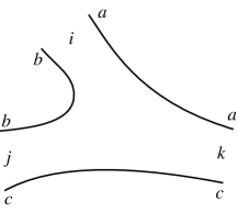
Figure 15: Cubic vertex for open strings.

For the special case $X={\cal C}$, where ${\cal C}$ denotes the conjugation matrix of the conformal theory, defined by

$$S^{2}=P^{2}=(S\,T)^{3}=\cal C\,,$$ (515)

and provided the boundaries respect the maximal symmetry of the bulk, Cardy [46] uncovered an important link between ${\cal A}$ and the fusion-rule coefficients that, in retrospect, may be regarded as the very rationale for the fusion algebra (506). His argument can be justified by the string-inspired picture of the merging of a pair of open strings at a cubic vertex, as in figure 15, noticing that if $X={\cal C}$ all closed-string sectors can reflect at the two boundaries, so that in this case there are as many independent reflection coefficients, or boundary labels $(a,b,c)$, as holomorphic bulk labels or, equivalently, sectors of the bulk spectrum $(i,j,k)$. As a result, in this case the number of charge sectors is also equal to the number of bulk sectors, while on the one hand the fusion-rule coefficients ${\cal N}_{ij}{}^{k}$ have the right structure to count string states in sector $i$ with a pair of boundaries labelled by $j$ and $k$, and on the other hand they fuse together, as in eq. (506), like open strings should. Moreover, if one identifies the annulus coefficients with the ${\cal N}_{ij}{}^{k}$, writing

$${\cal A}={\textstyle\frac{1}{2}}\sum_{i,j,k}{\cal N}_{ij}{}^{k}\,n^{i}\,n^{j}\,\chi_{k}\,,$$ (516)

the Verlinde formula guarantees that

$$\tilde{\cal A}={\textstyle\frac{1}{2}}\sum_{i}\,\chi_{i}\left(\sum_{j}\frac{S^{i}_{j}}{\sqrt{S^{i}_{1}}}n^{j}\right)^{2}$$ (517)

has the proper structure (513), while determining the $B_{a}^{i}$ in terms of the $S$ matrix. This structure, as first observed in [47], is instrumental in allowing consistent Möbius projections.

We can actually move a bit further, supplementing ${\cal A}$ with corresponding Klein-bottle and Möbius amplitudes. However, as we have seen in several examples, these choices are not unique in general, and Cardy’s Ansatz in terms of independent charge sectors applies only to the canonical choice

$$\tilde{\cal K} = {\textstyle{1\over 2}}\sum_{i}\,\chi_{i}\,{\biggl{(}{{P_{1i}}\over{\sqrt{S_{1i}}}}\biggr{)}}^{2}\,,$$ (518)

$$\tilde{\cal M}\ = \ \pm\,{\textstyle{1\over 2}}\ \sum_{i,j}\ \hat{\chi}_{i}\ \biggl{(}{{P_{1i}\ S_{ij}\ n^{j}}\over{S_{1i}}}\biggr{)}\,,$$ (519)

where the crosscap one-point functions can be expressed in terms of the first line of $P$ in a way reminiscent of Cardy’s relation between the boundary coefficients and the $S$ matrix [56, 57] while, turning to the direct channel,

$${\cal K}={\textstyle{1\over 2}}\ \sum_{i}\,{\cal Y}^{i}{}_{1}{}^{1}\,\chi_{i}$$ (520)

and

$${\cal M}=\pm\,{\textstyle{1\over 2}}\ \sum_{i,j}\,{\cal Y}_{j1}{}^{i}\ n^{j}\hat{\chi}_{i}\,,$$ (521)

are both expressible in terms of the first line of the ${\cal Y}_{i}$ matrices. These results admit interesting generalizations to cases where boundaries and crosscaps preserve only part of the bulk symmetry [171], that correspond to allowing (discrete) deformations of the types described in the previous section in the geometries underlying these rational constructions.

6.1 The ten-dimensional models revisited

In section 3 we have already met the open descendants of the ten-dimensional 0A and 0B models. We can now revisit them, since they give us an opportunity to exhibit the structure of Boundary Conformal Field Theory in a very simple setting. To this end, one must turn to the properly redefined basis, $\{V_{8},O_{8},-S_{8},-C_{8}\}$, already introduced in subsection 3.1, that accounts for the spin-statistics relation [27]. Since these examples are actually critical string models, we can well retain the various overall coefficients introduced by the modular integrals. One can also note that in this case the explicit expressions for $S$ and $P$ in eqs. (134) and (137) imply that for this class of models

$${\cal Y}_{ij}{}^{k}=S_{jk}\,\delta_{i}{}^{k}\,,$$ (522)

while ${\cal C}=1_{4}$, and therefore all indices can be raised and lowered at no cost. The 0B descendants associated to ${\cal K}_{1}$ are the simplest ones in this respect, since their annulus amplitude is precisely of Cardy type, while ${\cal K}_{1}$ and ${\cal M}_{1}$ are precisely as in eqs. (520) and (521). The other descendants of [58] reviewed in section 3 can then be recovered replacing the fixed indices, equal to 1 in (520) and (521), with 2,3 and 4, although the last two choices are connected by an overall parity transformation. The charge assignments in ${\cal A}$ change accordingly, in a simple and amusing fashion, so that

$${\cal A}_{(l)}={\textstyle\frac{1}{2}}\sum_{i,j,k}{\cal N}_{jk}{}^{i}\,n^{j}\,n^{k}\,\chi_{[i]\times[l]}\,,$$ (523)

but this introduces a slight subtlety, since the new Chan-Paton multiplicities form conjugate pairs, corresponding to the product of two unitary gauge groups, as we already saw in section 3.

On the other hand, the 0A model is not of Cardy type, and it is simple to convince oneself that in this case there are two charges, since only two bulk sectors, $V_{8}$ and $O_{8}$, can flow in the transverse channel. Thus, at best one can start from [47, 48]

$$\tilde{\cal A}=\frac{2^{-5}}{2}\,\left(\alpha^{2}O_{8}+\beta^{2}V_{8}\right)\,,$$ (524)

that reverting to the direct channel gives

$${\cal A}={\textstyle\frac{1}{4}}\,\left[(\alpha^{2}+\beta^{2})\,(O_{8}+V_{8})-(\beta^{2}-\alpha^{2})\,(S_{8}+C_{8})\right]\,,$$ (525)

while now the transverse Klein bottle

$$\tilde{\cal K}=\frac{2^{5}}{2}(O_{8}+V_{8})$$ (526)

and the annulus of eq. (524) imply that

$$\tilde{\cal M}=\alpha\hat{O}_{8}+\beta\hat{V}_{8}\,,$$ (527)

and thus, after a $P$ transformation and the usual redefinition of the measure, that

$${\cal M}={\textstyle{1\over 2}}\left(-\alpha\,\hat{O}_{8}+\beta\,\hat{V}_{8}\right)\,.$$ (528)

In section 3 we have already come to this point, and we have actually completed the construction introducing a parametrization in terms of two real Chan-Paton multiplicities,

$$\alpha=n_{B}-n_{F}\,,\qquad\beta=n_{B}+n_{F}\,.$$ (529)

We now want to see how this result can be retrieved following two different, albeit equally instructive, routes.

The first derivation is based on the link between the 0B and 0A models, similar to that between the IIB and IIA strings, so that one can recover the latter as a $(-1)^{F_{\rm L}}$ orbifold of the former, where $F_{\rm L}$ denotes the left space-time fermion number. This operation reverses all R-R fields, inducing the interchange of branes and antibranes, a symmetry only if they occur in equal numbers, i.e. if $n_{o}\equiv n_{v}$ and $n_{s}\equiv n_{c}$. After an overall rescaling, that in space-time language recovers the correct brane tension, identifying the former with $n_{B}$ and the latter with $n_{F}$ yields the annulus amplitude in eq. (170) or, equivalently, the parametrization in (529). The corresponding Möbius amplitude, however, cannot be obtained in this way, since now ${\cal K}$ is also modified, but it can be directly recovered from $\tilde{\cal A}$ and $\tilde{\cal K}$. Actually, in this particular case

$${\cal M}=\pm\,{\textstyle{1\over 2}}\,\sum_{i,j}\,\;\frac{{\cal Y}_{1j}{}^{i}+{\cal Y}_{2j}{}^{i}}{2}\;n^{j}\,\hat{\chi}_{i}\,,$$ (530)

where the multiplicities are to be identified as above. This setting is typical of off-diagonal models where no fixed points are introduced by the identifications, an additional subtlety nicely illustrated by the $D_{\rm odd}$ SU(2) WZW models, that we shall discuss in the last subsection.

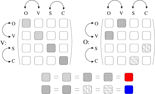
Figure 16: Chan-Paton matrices for the 0A orientifold.

This derivation has the additional virtue of revealing the precise link between the Chan-Paton assignments of the two models. For instance, the matrices for the $V_{8}$ and $O_{8}$ sectors of the 0B descendant of eq. (176) are depicted in figure 16. As we have seen, the $(-1)^{F_{\rm L}}$ orbifold brings about the conditions $n_{o}\equiv n_{v}$ and $n_{s}\equiv n_{c}$, necessary for a consistent 0A partition function. These effectively identify pairs of quantum numbers that were originally distinct, but the resulting Chan-Paton matrices for the $O_{8}$ and $V_{8}$ and $S_{8}$ and $C_{8}$ sectors of the 0A model are still distinct. It is amusing to see how a close scrutiny of the partition functions can exhibit this peculiarity, first noticed in [115]. Similar considerations apply to other models obtained as orbifolds of Cardy-like ones.

The second derivation, on the other hand, is meant to illustrate in the simplest possible setting a constructive algorithm, of general applicability in rational models, that uses ${\cal M}$ to linearize the constraints on the charge multiplicities. It results in a set of Diophantine equations that are solved by small signed integers, and whose solutions can thus be found by trial and error. The basic trick is to “turn on one charge at a time” [56, 57]. All terms in ${\cal A}$ and ${\cal M}$ are then to be equal modulo 2, as can be seen specializing any of our previous amplitudes, while ${\cal M}$, being linear in the charge multiplicities, allows a superposition of the independent solutions to the resulting Diophantine constraints. Our starting point in this case is then [47, 48]

$${\cal M} = {\textstyle\frac{1}{2}}\,\left(-\alpha\hat{O}_{8}+\beta\hat{V}_{8}\right)\,,$$

$$\tilde{\cal M} = \alpha\hat{O}_{8}+\beta\hat{V}_{8}\,,$$ (531)

where we must express $\alpha$ and $\beta$ in terms of two multiplicities $n_{B}$ and $n_{F}$ as

$$\alpha = a_{1}n_{B}+a_{2}n_{F}\,,$$

$$\beta = b_{1}n_{B}+b_{2}n_{F}\,,$$ (532)

with the $a_{i}$’s and $b_{i}$’s the signed integers to be determined. We now proceed in a slightly different order with respect to the previous cases, and use $\tilde{\cal M}$ to derive

$$\tilde{\cal A} = \frac{2^{-5}}{2}\left[(a_{1}n_{B}+a_{2}n_{F})^{2}O_{8}+(b_{1}n_{B}+b_{2}n_{F})^{2}V_{8}\right]\,,$$

$${\cal A} = {\textstyle\frac{1}{4}}\bigl{\{}\left[(a_{1}n_{B}+a_{2}n_{F})^{2}+(b_{1}n_{B}+b_{2}n_{F})^{2}\right](O_{8}+V_{8})$$ (533)

$$-\left[-(a_{1}n_{B}+a_{2}n_{F})^{2}+(b_{1}n_{B}+b_{2}n_{F})^{2}\right](S_{8}+C_{8})\bigr{\}}\,.$$

Next we let $n_{B}=1$ and $n_{F}=0$, and demand that, within this single-charge assignment, the contributions in ${\cal A}$ and ${\cal M}$ be equal modulo two. This gives the conditions

$$b_{1}^{2}=a_{1}^{2}\,,\qquad{\textstyle\frac{1}{2}}(a_{1}^{2}+b_{1}^{2})=a_{1}\ {\rm mod}\ 2\,,\qquad{\textstyle\frac{1}{2}}(a_{1}^{2}+b_{1}^{2})=b_{1}\ {\rm mod}\ 2\,,$$ (534)

that clearly admit the four solutions $a_{1}=b_{1}=\pm 1$ $a_{1}=-b_{1}=\pm 1$, two of which can be obtained from the others by the usual overall reversal of ${\cal M}$, while the choice $n_{B}=0$, $n_{F}=1$ leads again to these solutions. The general solution can then be obtained superposing an independent pair of these, say $a_{1}=b_{1}=b_{2}=1$, $a_{2}=-1$, so that, as before

$${\cal A} = {\textstyle\frac{1}{2}}(n_{B}^{2}+n_{F}^{2})(O_{8}+V_{8})-n_{B}n_{F}(S_{8}+C_{8})\,,$$

$${\cal M} = -{\textstyle{1\over 2}}(n_{B}-n_{F})\hat{O}_{8}+{\textstyle{1\over 2}}(n_{B}+n_{F})\hat{V}_{8}\,.$$ (535)

Notice that the restriction to the orientifold can be simply relaxed, so that the oriented D9 brane spectrum of the “parent” 0A model,

$$\tilde{\cal A} = \frac{2^{-5}}{2}\left[|n_{B}+n_{F}|^{2}V_{8}+|n_{B}-n_{F}|^{2}O_{8}\right]\,,$$

$${\cal A} = (n_{B}\bar{n}_{B}+n_{F}\bar{n}_{F})(O_{8}+V_{8})-(n_{B}\bar{n}_{F}+n_{F}\bar{n}_{B})(S_{8}+C_{8})$$ (536)

can be recovered complexifying all multiplicities, as in the previous section. In analogy with our discussion of subsection 5.12, these amplitudes also describe uncharged branes of the 0B string.

Although this is a non-diagonal model, the algorithm was somewhat simplified in this example, since $\tilde{\cal A}$ and $\tilde{\cal M}$ allow the same types of sectors. When $\tilde{\cal A}$ admits additional sectors, these behave like twisted orbifold projections, that split different charge sectors. We shall return to this point in the last subsection, after a cursory review of the SU(2) WZW models. This method is quite effective: it led to the first derivation of the boundary-operator spectrum for the $D_{\rm odd}$ series [56, 57], a result later generalized in [172] and recovered in [170] by a direct construction based on the ADE adjacency matrices.

6.2 Rational models and tensor multiplets in six dimensions

It is also instructive to reconsider some lower-dimensional string models from the viewpoint of Rational Conformal Field Theory. For the sake of brevity, we shall confine our attention to the simplest class of six-dimensional rational orbifolds, that can be obtained as $\hbox{\mbm Z}_{2}$ orbifolds of the toroidal compactification on the SO(8) lattice. Our starting point is then

$${\cal T}=|V_{8}-S_{8}|^{2}\,\left(|O_{8}|^{2}+|V_{8}|^{2}+|S_{8}|^{2}+|C_{8}|^{2}\right)\,.$$ (537)

The internal SO(8) partition function corresponds to a lattice whose metric is given by the $D_{4}$ Cartan matrix, and that includes

$$B=\frac{\alpha^{\prime}}{2}\,\left(\begin{array}[]{rrrr}0&1&0&0\\ -1&0&1&1\\ 0&-1&0&0\\ 0&-1&0&0\end{array}\right)\,,$$ (538)

a quantized $B_{ab}$ of rank $r=2$, determined by the corresponding adjacency matrix. The results of section 4 thus imply that a toroidal compactification on this lattice should give a Chan-Paton gauge group of rank 8. Indeed the Klein bottle, annulus and Möbius amplitudes

$${\cal K} = {\textstyle\frac{1}{2}}\,\left(V_{8}-S_{8}\right)\,\left(O_{8}+V_{8}+S_{8}+C_{8}\right)\,,$$

$${\cal A} = \frac{N^{2}}{2}\,\left(V_{8}-S_{8}\right)\,O_{8}\,,$$

$${\cal M} = \frac{N}{2}\,(\hat{V}_{8}-\hat{S}_{8})\,\hat{O}_{8}\,,$$ (539)

and the corresponding transverse-channel amplitudes

$$\tilde{\cal K} = \frac{2^{4}}{2}\,\left(V_{8}-S_{8}\right)\,O_{8}\,,$$

$$\tilde{\cal A} = \frac{2^{-4}\,N^{2}}{2}\,\left(V_{8}-S_{8}\right)\,\left(O_{8}+V_{8}+S_{8}+C_{8}\right)\,,$$

$$\tilde{\cal M} = -N\,(\hat{V}_{8}-\hat{S}_{8})\,\hat{O}_{8}\,,$$ (540)

define a consistent spectrum with a ${\rm USp}(16)$ gauge group. Although simply implied by the $P$ matrix of eq. (137) for SO(4) characters, that interchanges $\hat{O}_{4}$ and $\hat{V}_{4}$, the USp(16) gauge group of this model was in itself a surprise in a toroidal compactification of the SO(32) superstring [47, 48]. In section 4 we have already seen how a quantized $B_{ab}$ is accompanied by symplectic and orthogonal groups at the end points of continuous Wilson lines connecting $\gamma$ coefficients of opposite signs, as in subsection 4.2. In this rational setting, this peculiar effect manifests itself as a discrete deformation of the Möbius amplitude. The basic idea [48] is that relative phases between boundaries and crosscaps can alter the lattice contribution to $\tilde{\cal M}$, so that while the natural choice would be

$$\hat{O}_{8}=\hat{O}_{4}\hat{O}_{4}-\hat{V}_{4}\hat{V}_{4}\,,$$ (541)

where the relative sign between the two terms reflects their different conformal weights, one could also start from

$$\tilde{\cal M}=-N\,(\hat{V}_{8}-\hat{S}_{8})\,(\hat{O}_{4}\hat{O}_{4}+\hat{V}_{4}\hat{V}_{4})\,.$$ (542)

The different choice of twist would have a very clear effect in the direct-channel amplitude

$${\cal M}=-\frac{N}{2}\,(\hat{V}_{8}-\hat{S}_{8})\,(\hat{O}_{4}\hat{O}_{4}+\hat{V}_{4}\hat{V}_{4})\,,$$ (543)

determined by the SO(4) $P$ matrix of eq. (142), that would antisymmetrize the vector, yielding an SO(16) gauge group. These multiple choices were referred to in [48] as “discrete Wilson lines” in ${\cal M}$.

Constructing $\hbox{\mbm Z}_{2}$ orbifolds of this model is also quite simple and rewarding, for they capture the most striking feature of six-dimensional type I vacua, the generic presence of several tensor multiplets [47, 48]. All one needs is to combine the breaking of the space-time characters with a proper action on the internal ones compatible with the world-sheet supercurrent, and this is simply achieved in this case if the internal SO(8) is broken to ${\rm SO}(4)\times{\rm SO}(4)$. The resulting models contain a total of sixteen characters $\chi_{i}$, all listed in table 13, whose $S$ and $P$ matrices

$${\tiny S=\frac{1}{4}\,\left(\begin{array}[]{rrrrrrrrrrrrrrrr}+&+&+&+&+&+&+&+&+&+&+&+&+&+&+&+\\ +&+&-&-&+&+&-&-&+&+&-&-&+&+&-&-\\ +&-&+&-&+&-&+&-&+&-&+&-&+&-&+&-\\ +&-&-&+&+&-&-&+&+&-&-&+&+&-&-&+\\ +&+&+&+&+&+&+&+&-&-&-&-&-&-&-&-\\ +&+&-&-&+&+&-&-&-&-&+&+&-&-&+&+\\ +&-&+&-&+&-&+&-&-&+&-&+&-&+&-&+\\ +&-&-&+&+&-&-&+&-&+&+&-&-&+&+&-\\ +&+&+&+&-&-&-&-&+&+&+&+&-&-&-&-\\ +&+&-&-&-&-&+&+&+&+&-&-&-&-&+&+\\ +&-&+&-&-&+&-&+&+&-&+&-&-&+&-&+\\ +&-&-&+&-&+&+&-&+&-&-&+&-&+&+&-\\ +&+&+&+&-&-&-&-&-&-&-&-&+&+&+&+\\ +&+&-&-&-&-&+&+&-&-&+&+&+&+&-&-\\ +&-&+&-&-&+&-&+&-&+&-&+&+&-&+&-\\ +&-&-&+&-&+&+&-&-&+&+&-&+&-&-&+\end{array}\right)\,,}$$ (544)

$$P={\rm diag}(-,+,+,+,-,+,+,+,-,+,+,+,+,-,-,-)\,,$$ (545)

are, up to an overall normalization for $S$, just collections of signs. In particular, the diagonal modular invariant

$${\cal T}=\sum_{i=1}^{16}\;|\chi_{i}|^{2}$$ (546)

recovers the unique (2,0) supersymmetric anomaly-free massless spectrum of [110]. This comprises the gravitational multiplet and 21 tensor multiplets: one from $|\chi_{1}|^{2}$, four from $|\chi_{5}|^{2}$, and four from each of the twisted terms $|\chi_{9}|^{2}$, $|\chi_{14}|^{2}$, $|\chi_{15}|^{2}$ and $|\chi_{16}|^{2}$. As in the previous sections, let us begin by discussing the simplest Klein-bottle projection

$${\cal K}={\textstyle{1\over 2}}\sum_{i=1}^{16}\;\chi_{i}\,,$$ (547)

that determines a (1,0) massless spectrum comprising the gravitational multiplet, sixteen hyper multiplets, twelve of which originate from the twisted sector, and five tensor multiplets, four of which originate from the twisted sector. This was a major surprise of the original construction in [47, 48], since a naïve K3 reduction of the type I superstring would yield only one antisymmetric two-tensor. This oddity presents itself since the combination of orientifold and orbifold projections brings back into the physical spectrum remnants of the self-dual four-form of type IIB, although this field was projected out in ten-dimensions. As we have seen in the previous section, the twisted tensors signal the presence of ${\rm O}_{-}$ planes in the background [53]. Notice also how the fixed-point contributions occur in groups of four, consistently with the discussion of subsection 5.7 for the case $r=2$. In addition, from the four corresponding (2,0) tensor multiplets ${\cal K}$ extracts one (1,0) tensor multiplet and three (1,0) hypermultiplets, consistently with the presence of three ${\rm O}_{+}$ and one ${\rm O}_{-}$.

Table 13: Characters for the ${\rm SO}(8)/\hbox{\smbm Z}_{2}$ orbifold. At the massless level, $\chi_{1}$ contains a vector multiplet, $\chi_{5}$ a hyper multiplet, and $\chi_{9}$, $\chi_{14}$, $\chi_{15}$ and $\chi_{16}$ one half of a hyper multiplet each. The remaining characters contain only massive modes.

• $\chi_{1}=Q_{o}O_{4}O_{4}+Q_{v}V_{4}V_{4}$		$\chi_{9}\;\,=Q_{s}S_{4}O_{4}+Q_{c}C_{4}V_{4}$
  $\chi_{2}=Q_{o}O_{4}V_{4}+Q_{v}V_{4}O_{4}$		$\chi_{10}=Q_{s}S_{4}V_{4}+Q_{c}C_{4}O_{4}$
  $\chi_{3}=Q_{o}C_{4}C_{4}+Q_{v}S_{4}S_{4}$		$\chi_{11}=Q_{s}V_{4}C_{4}+Q_{c}O_{4}S_{4}$
  $\chi_{4}=Q_{o}C_{4}S_{4}+Q_{v}S_{4}C_{4}$		$\chi_{12}=Q_{s}V_{4}S_{4}+Q_{c}O_{4}C_{4}$
  $\chi_{5}=Q_{o}V_{4}V_{4}+Q_{v}O_{4}O_{4}$		$\chi_{13}=Q_{s}C_{4}V_{4}+Q_{c}S_{4}O_{4}$
  $\chi_{6}=Q_{o}V_{4}O_{4}+Q_{v}O_{4}V_{4}$		$\chi_{14}=Q_{s}C_{4}O_{4}+Q_{c}S_{4}V_{4}$
  $\chi_{7}=Q_{o}S_{4}S_{4}+Q_{v}C_{4}C_{4}$		$\chi_{15}=Q_{s}O_{4}S_{4}+Q_{c}V_{4}C_{4}$
  $\chi_{8}=Q_{o}S_{4}C_{4}+Q_{v}C_{4}S_{4}$		$\chi_{16}=Q_{s}O_{4}C_{4}+Q_{c}V_{4}S_{4}$

Notice that (546) is a diagonal modular invariant, a Cardy-like torus amplitude, and in analogy with the previous ten-dimensional type 0 examples one can then write

$${\cal A} = {\textstyle{1\over 2}}\sum_{i,j,k=1}^{16}\,{\cal N}_{ij}{}^{k}\,n^{i}\,n^{j}\,\chi_{k}\,,$$

$${\cal M} = {\textstyle{1\over 2}}\sum_{i,k=1}^{16}\,{\cal Y}_{1j}{}^{k}\,n^{i}\,\hat{\chi}_{k}\,.$$ (548)

The simplest solution of the resulting tadpole conditions involves four types of real multiplicities and results in the gauge group ${\rm USp}(8)\times{\rm USp}(8)\times{\rm USp}(8)\times{\rm USp}(8)$, with hyper multiplets in bi-fundamentals. This is the model where the generalized Green-Schwarz mechanism was first noticed [49], since here the reducible anomaly polynomial does not factorize as in the ten-dimensional SO(32) superstring [7], but can nonetheless be reduced to a sum of independent contributions that induce new two-form couplings in the low-energy model. In this case, the discrete Wilson lines of [48] can turn symplectic groups into unitary ones, and one can obtain a similar model with a ${\rm U}(8)\times{\rm U}(8)$ gauge group and hyper multiplets in antisymmetric and bi-fundamental representations. The two choices correspond to the two different signs for the $\xi$ coefficient of subsection 5.7, while the two models described are among those in tables 3 and 2.

As for the ten-dimensional models, the $P$ and $T$ matrices are identical diagonal collections of signs, and as a result the ${\cal Y}_{i}$ matrices, also diagonal, are related to the $S$ matrix as in (522). Further, for all allowed Klein bottles, $\tilde{\cal K}$ contains a single character, identified by the fixed index of ${\cal Y}$ and, as a result, there are three additional classes of models, according to whether this corresponds to a massive character, to $\chi_{5}$ or to one of the massless twisted ones. In the first case, the tadpole conditions imply that the model is consistent without an open sector, and indeed the corresponding projected closed spectrum is the only anomaly free one, with nine tensor multiplets and twelve hyper multiplets [141, 125, 124], while naïvely the second class of models appears to be inconsistent. We have already come across this type of models, since this setting is precisely what led to brane supersymmetry breaking in six dimensions in subsection 5.8. As in that case, we cannot proceed if we insist on working with the supersymmetric characters in the table. Rather, in $\tilde{\cal A}$ we should separate the NS and R contributions and, if this is done, all R-R tadpoles can be cancelled, while the resulting anomaly-free massless spectra are accompanied by a dilaton tadpole. Finally, the third class of models has the peculiar feature of having twisted tadpoles in $\tilde{\cal K}$, so that their open spectra are bound to involve collections of fractional branes that are neutral with respect to the untwisted R-R charges [75]. As an example let us consider the model associated to ${\cal Y}_{9}$, whose Klein-bottle amplitude

$${\cal K}={\textstyle{1\over 2}}\sum_{k=1}^{16}{\cal Y}^{k}{}_{9}{}^{9}\,\chi_{k}$$ (549)

yields a projected spectrum comprising the gravitational multiplet, thirteen tensor multiplets and eight hyper multiplets. This closed spectrum is anomalous, consistently with the fact that the transverse-channel Klein bottle amplitude

$$\tilde{\cal K}={2^{5}\over 2}\,\chi_{9}$$ (550)

develops a non-vanishing R-R tadpole but, differently from the previous cases, the massless tadpole now corresponds to a twisted character. As a result, the brane configuration should involve net numbers of fractional branes with no net untwisted R-R charge, and whose twisted charges should cancel locally the contribution of $\tilde{\cal K}$.

As for the original “brane supersymmetry breaking” model of [77], the construction of the open descendants must be slightly modified, since the direct-channel open-string amplitudes must include new sectors corresponding to brane-antibrane strings, that involve different GSO projections [75]. The transverse-channel annulus amplitude, however, can be easily obtained from the Cardy case, if the R portions of the characters are fused with the NS part corresponding to the new index, ‘9’ in our case, of the ${\cal Y}$-tensor present in ${\cal K}$,

$$\tilde{\cal A}={2^{-5}\over 2}\sum_{i=1}^{16}\epsilon_{i}\left(\sum_{j=1}^{16}S_{ij}n^{j}\right)^{2}\,\left(\chi_{i}^{\rm NS}+\chi^{\rm R}_{[i]\times[9]}\right)\,,$$ (551)

where the signs $\epsilon_{i}$, equal to $S_{i9}$ for the model we are considering, have to be introduced in order to guarantee a consistent interpretation for the direct-channel amplitudes, and imply that charge multiplicities form complex pairs. By standard methods one can then write

$$\tilde{\cal M}=-(n_{1}+n_{5}+n_{9}+n_{13})\,\hat{\chi}_{9}^{\rm R}-(n_{1}-n_{5}+n_{9}-n_{13})\,\hat{\chi}_{9}^{\rm NS}\,,$$ (552)

where we have introduced a minimal set of Chan-Paton multiplicities, that are to be subjected to the R-R tadpole conditions

$$n_{1}+n_{5}+n_{9}+n_{13} = 32\,,$$

$$n_{1}+n_{5}-n_{9}-n_{13} = 0\,,$$

$$n_{1}-n_{5}+n_{9}-n_{13} = 0\,,$$

$$n_{1}-n_{5}-n_{9}+n_{13} = 0\,.$$ (553)

Finally, $S$ and $P$ modular transformations and a suitable relabelling of the multiplicities,

$$n_{1}=n\,,\quad n_{9}=\bar{n}\,,\quad n_{5}=m\,,\quad n_{13}=\bar{m}\,,$$ (554)

give the direct-channel amplitudes

$${\cal A} = (n\bar{n}+m\bar{m})\chi_{1}+(n\bar{m}+\bar{n}m)\tilde{\chi}_{1}$$ (555)

$$+{\textstyle{1\over 2}}(n^{2}+\bar{n}^{2}+m^{2}+\bar{m}^{2})\chi_{9}+(nm+\bar{n}\bar{m})\tilde{\chi}_{9}\,,$$

and

$${\cal M}=(n+\bar{n})\,(\chi_{9}^{\rm NS}+\chi_{9}^{\rm R})-(m+\bar{m})\,(\chi_{9}^{\rm NS}-\chi_{9}^{\rm R})\,,$$ (556)

where, as in section 5, new combinations

$$\tilde{\chi}_{1} = (V_{4}V_{4}-C_{4}S_{4})O_{4}O_{4}+(O_{4}O_{4}-S_{4}C_{4})V_{4}V_{4}\,,$$

$$\tilde{\chi}_{9} = (O_{4}S_{4}-S_{4}V_{4})S_{4}O_{4}+(V_{4}C_{4}-C_{4}O_{4})C_{4}V_{4}\,,$$ (557)

pertain to open strings stretched between branes and antibranes. Notice the absence of the $\chi_{5}$ character, that contains the internal components of the brane gauge field, and whose presence would signal the possibility of displacing the branes, a reflection of the fact that the model indeed contains fractional branes. The tadpole conditions determine a ${\rm U}(8)\times{\rm U}(8)$ gauge group, and the model is free of gauge and gravitational anomalies.

One might conclude that, despite the simultaneous presence of branes and antibranes of the same type, the model be stable, since no tachyons are present while apparently the branes cannot be displaced. The detailed analysis of similar orientifolds [75], however, indicates that this should not be the case. In fact, although one is considering fractional branes, that cannot be moved away from the fixed points, there are still closed-string moduli related to the compactification torus. Tilting the $T^{4}$ alters the distance between brane-antibrane pairs, modifying the mass of the corresponding open-string states and, as a result, tachyons can indeed appear for some values of the geometric moduli. They reflect the stresses on the background geometry, and indeed these brane configurations can decay into magnetized (non-)BPS branes [75].

6.3 Examples from WZW models

These constructions apply directly to more complicated, interacting rational conformal theories, and we would like to conclude this review with some examples drawn from [56, 57]. These have the virtue of illustrating several new features in a relatively simple context, but the techniques apply with essentially no modifications to more physical, if more involved, settings, that describe branes in genuinely curved critical string backgrounds. For instance, an early, interesting application to four-dimensional Gepner models can be found in [144].

The characters $\chi_{\alpha}$ for the level-$k$ SU(2) WZW model [173], with central charge

$$c=\frac{3k}{k+2}\,,$$ (558)

are $k+1$, have isospins $(\alpha-1)/2$ and conformal weights

$$h_{\alpha}=\frac{\alpha^{2}-1}{4(k+2)}\,.$$ (559)

The corresponding $S$ and $P$ matrices are

$$S_{\alpha\beta}=\sqrt{2\over{k+2}}\ \sin\left({{\pi\alpha\beta}\over{k+2}}\right)\,,$$ (560)

and [54, 56]

$$P_{\alpha\beta}={2\over{\sqrt{k+2}}}\ \sin\left({{\pi\alpha\beta}\over{2(k+2)}}\right)(E_{k}E_{\alpha+\beta}+O_{k}O_{\alpha+\beta})\,,$$ (561)

where $E$ and $O$ denote even and odd projectors, while the allowed modular invariants fall in the ADE classification of Cappelli, Itzykson and Zuber [174] and are summarized in table 14.

Table 14: The ADE modular invariants for the SU(2) WZW models.

• series	level	modular invariant
  $A_{k+1}$	$k$	$\sum_{{}^{\alpha=1}_{\alpha\in\hbox{\ssmbm Z}}}^{k+1}|\chi_{\alpha}|^{2}$
  $D_{2\ell+2}$	$k=4\ell$	$\sum_{{}^{\alpha=1}_{\alpha\in 2\hbox{\ssmbm Z}+1}}^{2\ell-1}|\chi_{\alpha}+\chi_{4\ell-\alpha}|^{2}+2|\chi_{2\ell}|^{2}$
  $D_{2\ell+1}$	$k=4\ell-2$	$\sum^{4\ell-1}_{{}^{\alpha=1}_{\alpha\in 2\hbox{\ssmbm Z}+1}}|\chi_{\alpha}|^{2}+|\chi_{2\ell-1}|^{2}+\sum^{2\ell-2}_{{}^{\alpha=2}_{\alpha\in 2\hbox{\ssmbm Z}}}(\bar{\chi}_{4\ell-2-\alpha}\chi_{\alpha}+\bar{\chi}_{\alpha}\chi_{4\ell-2-\alpha})$
  $E_{6}$	$k=10$	$|\chi_{0}+\chi_{6}|^{2}+|\chi_{3}+\chi_{7}|^{2}+|\chi_{4}+\chi_{10}|^{2}$
  $E_{7}$	$k=16$	$|\chi_{0}+\chi_{16}|^{2}+|\chi_{4}+\chi_{12}|^{2}+|\chi_{6}+\chi_{10}|^{2}+|\chi_{8}|^{2}$
  		$+(\bar{\chi}_{2}+\bar{\chi}_{14})\chi_{8}+\bar{\chi}_{8}(\chi_{2}+\chi_{14})$
  $E_{8}$	$k=28$	$|\chi_{0}+\chi_{10}+\chi_{18}+\chi_{28}|^{2}+|\chi_{6}+\chi_{12}+\chi_{16}+\chi_{22}|^{2}$

The modular invariants of the $A$ series are diagonal, the $D_{\rm even}$, $E_{6}$ and $E_{8}$ ones are Cardy-like, i.e. charge-conjugate in terms of the characters of suitably extended algebras, and finally the $D_{\rm odd}$ and $E_{7}$ modular invariants are off-diagonal. Notice that the $D_{\rm even}$ models present a fixed-point ambiguity, to be resolved as in [108] in order to apply the previous formalism.

For the $A$-series, one can show that there are two independent choices for ${\cal K}$ consistent with the positivity of $\tilde{\cal K}$. The first corresponds to the Cardy Ansatz, and in this case

$${\cal K}={\textstyle{1\over 2}}\sum_{\alpha=1}^{k+1}(-1)^{\alpha-1}\chi_{\alpha}$$ (562)

is the Frobenius-Schur indicator [27], so that all sectors of integer isospin are symmetrized, while those of half-odd-integer isospin are antisymmetrized. The corresponding direct-channel annulus amplitudes involve $k+1$ real charge multiplicities, and read

$${\cal A}={\textstyle{1\over 2}}\sum_{\alpha,\beta,\gamma}\,{\cal N}_{\alpha\beta}{}^{\gamma}\,n^{\alpha}\,n^{\beta}\,\chi_{\gamma}\,,$$ (563)

and

$${\cal M}=\pm{\textstyle{1\over 2}}\sum_{\alpha,\beta}\,(-1)^{\beta-1}\,(-1)^{{\alpha-1}\over 2}\ {\cal N}_{\beta\beta}{}^{\alpha}\,n^{\beta}\,\hat{\chi}_{\alpha}\,,$$ (564)

where for $k$ odd the overall sign of ${\cal M}$ can actually be reversed redefining the charge multiplicities according to $n^{\alpha}\leftrightarrow n^{k+2-\alpha}$. The alternative choice for the Klein-bottle projection,

$${\cal K}={\textstyle{1\over 2}}\sum_{\alpha=1}^{k+1}\,\chi_{\alpha}\,,$$ (565)

also allowed, results in the appearance of complex charges. If $k$ is even, the model contains an odd number of characters in $\tilde{\cal A}$, and thus an odd number of charges. The charge corresponding to the middle character $\chi_{(k+2)/2}$ stays real, while those corresponding to $\chi_{\alpha}$ and $\chi_{k+2-\alpha}$ form complex pairs. On the other hand, if $k$ is odd all charges fall into complex pairs. In both cases, all signs disappear from the Möbius projection, and the resulting open spectra are described by

$${\cal A}={\textstyle{1\over 2}}\sum_{\alpha,\beta,\gamma}\,{\cal N}_{\alpha\beta}{}^{\gamma}\,n^{\alpha}\,n^{\beta}\,\chi_{k+2-\gamma}$$ (566)

and

$${\cal M}=\pm{\textstyle{1\over 2}}\sum_{\alpha,\beta}\,{\cal N}_{\beta\beta}{}^{\alpha}\,n^{\beta}\,\hat{\chi}_{k+2-\alpha}\,.$$ (567)

As is usually the case when complex charges are present [47], pair-wise identifications are implicit in eqs. (566) and (567), and in these models $n^{k+2-\alpha}={\bar{n}}^{\alpha}$.

As in previous examples, the brane spectrum of the “parent” model can be simply recovered from the Cardy assignment, discarding ${\cal K}$ and ${\cal M}$ and complexifying the charge multiplicities in ${\cal A}$. Thus, in our case one would obtain

$${\cal A}=\sum_{\alpha,\beta,\gamma}\,{\cal N}_{\alpha}{}^{\beta\gamma}\,n^{\alpha}\,{\bar{n}}_{\beta}\,\chi_{\gamma}\,,$$ (568)

in terms of the multiplicities $n^{\alpha}$ and their conjugates ${\bar{n}}_{\alpha}$. The states of half-odd-integer isospin occur in $\tilde{\cal A}$ with couplings of both signs, that reflect the $\hbox{\mbm Z}_{2}$ symmetry of the models and mimic the R-R charges of D-branes. The models of the $A$-series describe strings propagating on the SU(2) group manifold [173], the three-sphere, and these open sectors also characterize the corresponding brane configurations, if all charges are taken to be complex. These are generally D2 branes stabilized by NS-NS fluxes on conjugacy classes [175], that are depicted symbolically in figure 17 as meridians of a two-sphere. In a similar fashion, the $D$-series also admits a geometrical interpretation in terms of the propagation on the ${\rm SO}(3)={\rm SU}(2)/\hbox{\mbm Z}_{2}$ group manifold, that in the figure would become symbolically the two-sphere with opposite points identified. The orientifold loci present in this and other WZW models can be given a similar geometric interpretation [177], that also recovers rather neatly the relative signs for the various charges present in the Möbius amplitude in (564). The recent literature contains several extensive analyses along these lines of other rational conformal models and of their orientifolds [178].

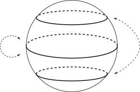
Figure 17: D-branes in the SU(2) and SO(3) WZW models.

The $D_{\rm even}$, $E_{6}$ and $E_{8}$ models are Cardy-like in terms of extended algebras, and as long as boundaries and crosscaps preserve them, the corresponding descendants can be obtained in a similar fashion, as in [56]. One novelty with respect to the previous case, introduced by the extended symmetry, is the occasional appearance in ${\cal A}$ and ${\cal M}$ of multiple sectors with identical types of charges. Following [56, 57], we can simply illustrate this phenomenon in the $k=16$ $D_{\rm even}$ model, while retaining for brevity only the two charges corresponding to the generalized characters $\chi_{c}=\chi_{5}+\chi_{13}$ and $\chi_{d}=\chi_{7}+\chi_{11}$. Letting $\chi_{a}=\chi_{1}+\chi_{17}$, $\chi_{b}=\chi_{3}+\chi_{15}$, denoting by $\chi_{e}$ and $\chi_{\tilde{e}}$ the two “resolved” characters and choosing for definiteness an overall positive sign for the Möbius amplitude, one gets

$${\cal A} = {{n_{c}^{2}+n_{d}^{2}}\over 2}\chi_{a}+\left({{n_{c}^{2}+n_{d}^{2}}\over 2}+\ n_{c}n_{d}\right)(\chi_{b}+\chi_{e}+\chi_{\tilde{e}})+$$ (569)

$$\left({{n_{c}^{2}+2n_{d}^{2}}\over 2}+n_{c}n_{d}\right)\chi_{c}+\left({{n_{c}^{2}+2n_{d}^{2}}\over 2}+2n_{c}n_{d}\right)\chi_{d}$$

and

$${\cal M}={{n_{c}+n_{d}}\over 2}(\hat{\chi}_{a}-\hat{\chi}_{b}+\hat{\chi}_{e}+\hat{\chi}_{\tilde{e}})+{{n_{c}+2n_{d}}\over 2}\hat{\chi}_{c}-{{n_{c}}\over 2}\hat{\chi}_{d}\,.$$ (570)

This example exhibits rather neatly three types of unconventional Chan-Paton multiplicities. The first presents itself in the open states described by $\chi_{c}$, where factors of two occur both in the annulus and in the Möbius amplitude for the charges of type $d$. There are thus two families of such states. The others present themselves in the open states corresponding to $\chi_{d}$, where the annulus amplitude contains factors of two for both $n_{d}^{2}$ and $n_{c}n_{d}$. Since in the Möbius amplitude $\chi_{d}$ does not appear with multiplicity $n_{d}$, there are two sectors of states with a pair of charges of type $d$, described by symmetric and antisymmetric matrices respectively. In addition, there are two sectors of states with a pair of distinct charges, of types $c$ and $d$. These multiple sets of states reflect the occurrence in these models of multiple three point functions, a consequence of the extended symmetry. We have already discussed two manifestations of the same phenomenon in subsections 5.11 and 5.12, when we described magnetized branes in the presence of a quantized $B_{ab}$ and non-BPS type I branes. If one allows the presence of boundaries that break the extended symmetry, the analogue in this context of what we saw for magnetized orbifolds or, more simply, for Wilson lines, the algorithm is more complicated, and for this more general case we refer the reader to [176], where the formalism was originally developed. A more refined mathematical framework for the whole construction, based on category theory, has also been recently proposed in [179], while the link between the Abelian Chern-Simons model and the conformal theory of free bosons in the presence of boundaries and crosscaps is discussed in [180].

We would like to conclude with a brief discussion of the $D_{\rm odd}$ models, particularly interesting since their partition functions are genuinely off-diagonal and contain simple currents of half-integer spin, while their open sectors display peculiar extensions similar to those in eq. (569). To this end, it suffices to consider the simplest of them, the $D_{5}$ model with $k=6$. In this case there are seven characters, $\chi_{1},\ldots,\chi_{7}$, with isospins from 0 to 3, and the partition function is

$${\cal T}_{D_{5}}=|\chi_{1}|^{2}+|\chi_{3}|^{2}+|\chi_{5}|^{2}+|\chi_{7}|^{2}+\chi_{2}\bar{\chi}_{6}+\chi_{6}\bar{\chi}_{2}+|\chi_{4}|^{2}\,,$$ (571)

while the corresponding diagonal $A$-series model is

$${\cal T}_{A_{6}}=|\chi_{1}|^{2}+|\chi_{2}|^{2}+|\chi_{3}|^{2}+|\chi_{4}|^{2}+|\chi_{5}|^{2}+|\chi_{6}|^{2}+|\chi_{7}|^{2}\,.$$ (572)

This pattern repeats for all the $D_{\rm odd}$ series, where the half-odd-integer isospin sectors form off-diagonal pairs of the type $\chi_{\alpha}\bar{\chi}_{k+2-\alpha}+{\rm h.c.}$, aside from the middle sector, that stays diagonal. In our case, starting from the seven charges of the $A_{6}$ model, we must end up with five charges in the $D_{5}$ one, as many as the sectors allowed in $\tilde{\cal A}$ in this case. There are again two descendants, one of which has all real charges. They were constructed with the algorithm discussed at the beginning of this section, turning on one charge at a time, and one type of charge was originally missed in [56], since this model actually presents multiplicities in ${\cal A}$ and ${\cal M}$ similar to those in the preceding $k=16$ example, that here can not be ascribed to bulk extensions, and were thus excluded. The proper result was then obtained in [57], where it was justified in terms of a set of polynomial equations for the rescaled boundary one-point functions

$$\tilde{B}_{i}^{a}=B_{i}^{a}\,\frac{\sqrt{S_{1i}}}{S_{1a}}\,,$$ (573)

a special case of the polynomial constraints that we mentioned at the beginning of this section. These reflect two limiting behaviours of the amplitude for two bulk fields in front of a boundary of type $a$ in figure 18, and read

$$\tilde{B}_{i}^{a}\,\tilde{B}_{j}^{a}=\sum_{k}\,\epsilon_{ij}{}^{k}\,{\cal N}_{ij}{}^{k}\,\tilde{B}_{k}^{a}\,,$$ (574)

where $\epsilon_{ij}{}^{k}$ is 1 for all $(i,j,k)$ in the diagonal case. On the other hand, in the off-diagonal case $\epsilon_{ij}{}^{k}$ is 1 when all three isospins are integer, while if two, say $i$ and $j$, are half-integer, it is $(-1)^{k}$. These quadratic constraints admit a number of distinct solutions, labelled by the index $a$, that correspond to the allowed boundary conditions, and illustrate the structure identified in [172] and termed there “classifying algebra of boundary conditions”. They can be simply solved for these two models yielding the results in table 15, whose last line corrects a misprint in [57]. Notice that pairs of $A_{6}$ one-point functions combine to give the $D_{5}$ ones, aside from that related to the middle field, that actually splits into two.

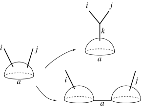
Figure 18: Limiting behaviours of two-point functions on a disk.

One can verify that, if all the corresponding charges are introduced, and only in this case, the annulus coefficients satisfy [57]

$$\sum_{b}{\cal A}^{i}{}_{a}{}^{b}\,{\cal A}^{j}{}_{bc} = \sum_{k}{\cal N}^{ij}{}_{k}\,{\cal A}^{k}{}_{ac}\,,$$ (575)

$$\sum_{i}{\cal A}_{iab}\,{\cal A}^{i}{}_{cd} = \sum_{i}{\cal A}_{iac}\,{\cal A}^{i}{}_{bd}\,.$$ (576)

The first equation is particularly interesting for, just like the ${\cal N}_{i}$’s and the ${\cal Y}_{i}$’s, the general annulus coefficients for off-diagonal amplitudes with reduced numbers of boundaries, determined by the states allowed in $\tilde{\cal A}$, satisfy the fusion algebra when they form a complete set. Actually, the completeness conditions (575) maintain the same form in more general settings, while the second equation only holds in the case at hand, where each character is associated to a different reflection coefficient. From a world-sheet perspective, as already stressed in the discussion of the Cardy case, eq. (575) embodies the key features of the three-point interaction, where a pair of open strings merge into a third one upon the disappearance of the common boundary and in fact, the original argument in [57], tailored for the case of boundaries of maximal symmetry, is a direct consequence of this picture. The recent literature also contains their extensions to the other amplitudes ${\cal K}$ and ${\cal M}$ [181]

$$\sum_{b}\,{\cal A}_{ia}{}^{b}\,{\cal M}_{jb} = \sum_{k}\,{\cal Y}_{ij}{}^{k}\,{\cal M}_{ka}\,,$$

$$\sum_{b}\,{\cal M}_{ib}\,{\cal M}^{jb} = \sum_{k}\,{\cal Y}_{ki}{}^{j}\,{\cal K}^{k}$$ (577)

with corresponding derivations [181, 170], especially in view of cases where boundaries break partly the bulk symmetry [176, 170]. One can actually show [181] that the additional Möbius-strip and Klein-bottle conditions (577), as well as similar ones for the most symmetric case, can be deduced, under plausible assumptions, from the completeness conditions (575). From the space-time viewpoint, these identify complete sets of branes, and are thus the analogue, in this context, of the modular invariance condition for bulk operators. Within our present understanding of String Theory, however, they clearly play a less prominent rôle, since branes are treated as classical objects whose fluctuations are quantized, as is usually the case for solitons in Field Theory. It is tempting to speculate, however, that a better understanding of String Theory will uncover the natural similarity between these completeness conditions for boundary operators and the modular invariance conditions for bulk spectra.

It is instructive to recover these assignments starting from the Cardy annulus for the $A_{6}$ model

$$\tilde{\cal A}_{6}\sim\sum_{\alpha}\,\frac{\chi_{\alpha}}{\sin\left(\frac{\pi\alpha}{8}\right)}\,\left|\,\sum_{\beta}\,\sin\left(\frac{\pi\alpha\beta}{8}\right)\,n_{\beta}\,\right|^{2}\ ,$$ (578)

determined by

$${\cal A}_{A_{6}}=\sum_{\alpha,\beta,\gamma}\,{{\cal N}_{\alpha}}{}^{\beta\gamma}\ n^{\alpha}\,\bar{n}_{\beta}\,\chi_{\gamma}\,,$$ (579)

and proceeding as in subsection 6.1, i.e.  identifying $n_{\alpha}$ and $n_{8-\alpha}$ and rescaling the overall tension. This procedure eliminates all boundary coefficients associated to sectors with half-odd-integer isospin, and reflects the derivation of the $D_{5}$ partition function as a $\hbox{\mbm Z}_{2}$ orbifold of (579) by $(-1)^{2I_{\rm L}}$, where $I_{\rm L}$ denotes the left isospin quantum number. One thus obtains

$${\cal A} = \left[n_{1}\bar{n}_{1}+n_{2}\bar{n}_{2}+n_{3}\bar{n}_{3}+\frac{n_{4}\bar{n}_{4}}{2}\right](\chi_{1}+\chi_{7})$$ (580)

$$+[n_{1}\bar{n}_{2}+n_{2}\bar{n}_{3}+n_{3}\bar{n}_{4}+{\rm h.c.}](\chi_{2}+\chi_{6})$$

$$+\left[n_{2}\bar{n}_{2}+2n_{3}\bar{n}_{3}+\frac{n_{4}\bar{n}_{4}}{2}+(n_{1}\bar{n}_{3}+n_{2}\bar{n}_{4}+{\rm h.c.})\right](\chi_{3}+\chi_{5})$$

$$+[n_{1}\bar{n}_{4}+2n_{2}\bar{n}_{3}+n_{3}\bar{n}_{4}+{\rm h.c.}]\chi_{4}\,,$$

that has apparently two problems. Firstly, there are only four charges, while their total number is expected to be five, since five sectors are allowed in $\tilde{\cal A}$, and moreover the terms involving $n_{4}$ do not afford a proper particle interpretation, since they are not properly normalized. This novelty originates from the fact that the identifications have a fixed point, represented in this case by the $\chi_{4}$ sector, that indeed corresponds to a twisted sector of the $D_{5}$ model, as can be seen from table 15 or from the derivation of the $D_{5}$ torus amplitude as an $A_{6}$ orbifold. The problems are indeed eliminated if in (580) $n_{4}$ is split into a pair of charges,

$$n_{4}\to n_{4}+n_{5}\,,$$ (581)

and a new contribution involving $\chi_{4}$ and proportional to $|n_{4}-n_{5}|^{2}$ is added to $\tilde{\cal A}$. This is allowed, since $\chi_{4}$ occurs diagonally in the $D_{5}$ model, and plays the rôle of the $R_{N,D}$ breaking terms of section 5. The end result,

$${\cal A}_{D_{5}} = \left[n_{1}\bar{n}_{1}+n_{2}\bar{n}_{2}+n_{3}\bar{n}_{3}+n_{4}\bar{n}_{4}+n_{5}\bar{n}_{5}\right]\chi_{1}$$ (582)

$$+\left[n_{1}\bar{n}_{2}+n_{2}\bar{n}_{3}+n_{3}\bar{n}_{4}+n_{3}\bar{n}_{5}+h.c.\right](\chi_{2}+\chi_{6})$$

$$+\left[n_{2}\bar{n}_{2}+2n_{3}\bar{n}_{3}+(n_{1}\bar{n}_{3}+n_{2}\bar{n}_{4}+n_{2}\bar{n}_{5}+n_{4}\bar{n}_{5}+h.c.)\right]\chi_{3}$$

$$+[n_{1}\bar{n}_{4}+n_{1}\bar{n}_{5}+2n_{2}\bar{n}_{3}+n_{3}\bar{n}_{4}+n_{3}\bar{n}_{5}+h.c]\chi_{4}$$

$$+\left[n_{2}\bar{n}_{2}+2n_{3}\bar{n}_{3}+n_{4}\bar{n}_{4}+n_{5}\bar{n}_{5}+(n_{1}\bar{n}_{3}+n_{2}\bar{n}_{4}+n_{2}\bar{n}_{5}+h.c.)\right]\chi_{5}$$

$$+\left[n_{1}\bar{n}_{1}+n_{2}\bar{n}_{2}+n_{3}\bar{n}_{3}+(n_{4}\bar{n}_{5}+h.c.)\right]\chi_{7}\,,$$

coincides with the orientifold annulus amplitude in [57], after the redefinitions $n_{\alpha}\to l_{\alpha}$, $l_{1}\leftrightarrow l_{2}$ and $l_{3}\leftrightarrow l_{5}$ and the restriction to real charges. From a geometric viewpoint, the branes in the $D_{\rm odd}$ case are those allowed in the SO(3) manifold, i.e. pairs of SU(2) branes with opposite latitude, aside from the equatorial one, that is fixed and actually splits into a pair of fractional branes. This geometric derivation of the $D_{\rm odd}$ models first appeared in [182], and was later recovered in these terms in [161, 183].

Table 15: Rescaled boundary coefficients for the $A_{6}$ and $D_{5}$ models.

$a$	$\tilde{B}_{1}^{a}$	$\tilde{B}_{3}^{a}$	$\tilde{B}_{5}^{a}$	$\tilde{B}_{7}^{a}$	$\tilde{B}_{4}^{a(A_{6})}$	$\tilde{B}_{2}^{a}$	$\tilde{B}_{6}^{a}$	$\tilde{B}_{4}^{a(D_{5})}$
$({\textstyle{1\over 2}},{\textstyle{5\over 2}})$	$1$	$1$	$-1$	$-1$	$0$	$\pm\sqrt{2}$	$\mp\sqrt{2}$	$0$
$({\textstyle{3\over 2}})$	$1$	$-1$	$1$	$-1$	$0$	$0$	$0$	$\pm 2$
$(0,3)$	$1$	$1+\sqrt{2}$	$1+\sqrt{2}$	$1$	$\pm\sqrt{2(2+\sqrt{2})}$	$\pm\sqrt{2+\sqrt{2}}$	$\pm\sqrt{2+\sqrt{2}}$	$0$
$(1,2)$	$1$	$1-\sqrt{2}$	$1-\sqrt{2}$	$1$	$\mp\sqrt{2(2-\sqrt{2})}$	$\pm\sqrt{2-\sqrt{2}}$	$\pm\sqrt{2-\sqrt{2}}$	$0$

References

References

- [1] G. Veneziano, “Construction of a crossing-symmetric, Regge behaved amplitude for linearly rising trajectories”, Nuovo Cim. A57 (1968) 190.
- [2] M. A. Virasoro, “Alternative constructions of crossing-symmetric amplitudes with Regge behavior”, Phys. Rev. 177 (1969) 2309; J. A. Shapiro, “Narrow-resonance model with Regge behavior for - scattering”, Phys. Rev. 179 (1969) 1345.
- [3] Z. Koba and H. B. Nielsen, “Reaction amplitude for mesons: a generalization of the Veneziano-Bardakci-Ruegg-Virasoro model”, Nucl. Phys. B10 (1969) 633, “Manifestly crossing invariant parametrization of meson amplitude”, Nucl. Phys. B12 (1969) 517.
- [4] A. Neveu and J. H. Schwarz, “Factorizable dual model of pions”, Nucl. Phys. B31 (1971) 86, “Quark model of dual pions”, Phys. Rev. D4 (1971) 1109; A. Neveu, J. H. Schwarz and C. B. Thorn, “Reformulation of the dual pion model”, Phys. Lett. B35 (1971) 529; P. Ramond, “An interpretation of dual theories”, Nuovo Cim. A4 (1971) 544, “Dual theory for free fermions”, Phys. Rev. D3 (1971) 2415,
- [5] “Dual Theory”, M. Jacob ed., Physics Reports Reprint Volume I (North-Holland, Amsterdam, 1974); J. Scherk, “An introduction to the theory of dual models and strings”, Rev. Mod. Phys. 47 (1975) 123.
- [6] J. Scherk and J. H. Schwarz, “Dual models for non-hadrons”, Nucl. Phys. B81 (1974) 118; T. Yoneya, “Connection of dual models to Electrodynamics and Gravidynamics”, Prog. Theor. Phys. 51 (1974) 1907.
- [7] M. B. Green and J. H. Schwarz, “Anomaly cancellation in supersymmetric gauge theory and superstring theory”, Phys. Lett. B149 (1984) 117.
- [8] R. P. Feynman, “Quantum theory of gravitation”, Acta Phys. Polon. 24 (1963) 697; B. S. Dewitt, “Quantum theory of gravity. II. The manifestly covariant theory”, Phys. Rev. 162 (1967) 1195; G. ’t Hooft and M. J. Veltman, “One loop divergencies in the theory of gravitation”, Annales Poincare Phys. Theor. A20 (1974) 69. M. H. Goroff and A. Sagnotti, “Quantum gravity at two loops”, Phys. Lett. B160 (1985) 81, “The ultraviolet behavior of Einstein gravity”, Nucl. Phys. B266 (1986) 709; A. E. van de Ven, “Two loop quantum gravity”, Nucl. Phys. B378 (1992) 309.
- [9] P. Candelas, G. T. Horowitz, A. Strominger and E. Witten, “Vacuum configurations for superstrings”, Nucl. Phys. B258 (1985) 46. For a recent review see, for instance: B. R. Greene, “String theory on Calabi-Yau manifolds”, arXiv:hep-th/9702155.
- [10] An unsurpassed book on many aspects of the subject, and in particular on Calabi-Yau compactifications, is: M.B. Green, J.H. Schwarz and E. Witten, Superstring Theory, 2 vols. (Cambridge Univ. Press, Cambridge, 1988). More recent books are: D. Lüst and S. Theisen, Lectures on String Theory, Lect. Notes Phys. 346 (1989) 1; E. Kiritsis, Introduction to Superstring Theory, (Leuven Univ. Press, Leuven, 1998) [arXiv:hep-th/9709062], and the more comprehensive J. Polchinski, String Theory, 2 vols. (Cambridge Univ. Press, Cambridge, 1999).
- [11] D. Z. Freedman, P. van Nieuwenhuizen and S. Ferrara, “Progress toward a theory of supergravity”, Phys. Rev. D13 (1976) 3214; S. Deser and B. Zumino, “Consistent supergravity”, Phys. Lett. B62 (1976) 335. For reviews and collections of reprints see, for instance: P. Van Nieuwenhuizen, “Supergravity”, Phys. Rept. 68 (1981) 189; S. Ferrara, Supersymmetry, 2 vols (World Scientific, Singapore, 1987); J. Bagger and J. Wess, Supersymmetry and supergravity. 2nd edition, (Princeton Univ. Press, Princeton, 1992); P.C. West, Introdution to supersymmetry and supergravity (World Scientific, Singapore, 1990); A. Salam and E. Sezgin, Supergravity in diverse dimensions, 2 vols (World Scientific, Singapore, 1989).
- [12] D. J. Gross, J. A. Harvey, E. J. Martinec and R. Rohm, “The heterotic string”, Phys. Rev. Lett. 54 (1985) 502, “Heterotic string theory. 1. The free heterotic string”, Nucl. Phys. B256 (1985) 253, “Heterotic string theory. 2. The interacting heterotic string”, Nucl. Phys. B267 (1986) 75.
- [13] The possibility of cancelling gauge and gravitational anomalies with the gauge group was first stressed in: J. Thierry-Mieg, “Remarks concerning the and string theories”, Phys. Lett. B156 (1985) 199.
- [14] K. Bardakci and M. B. Halpern, “New dual quark models”, Phys. Rev. D3 (1971) 2493; I. B. Frenkel and V. G. Kac, “Basic representations of affine Lie algebras and dual resonance models”, Invent. Math. 62 (1980) 23; P. Goddard and D. I. Olive, “Algebras, lattices and strings”, DAMTP-83/22 Talks given at the Workshop on Vertex Operators in Mathematics and Physics, Berkeley, Calif., “Kac-Moody algebras, conformal symmetry and critical exponents”, Nucl. Phys. B257 (1985) 226. For reviews, see, for instance: V. Kac, Infinite dimensional Lie Algebras (Cambridge Univ. Press, Cambridge, 1985); C. Itzykson and J.M. Drouffe, Statistical Field Theory (Cambridge Univ. Press, Cambridge, 1989).
- [15] J. E. Paton and H. M. Chan, “Generalized Veneziano model with isospin”, Nucl. Phys. B10 (1969) 516.
- [16] J. H. Schwarz, “Gauge groups for type I superstrings”, CALT-68-906-REV Presented at 6th Johns Hopkins Workshop on Current Problems in High-Energy Particle Theory, Florence, Italy, Jun 2-4, 1982; N. Marcus and A. Sagnotti, “Tree level constraints on gauge groups for type I superstrings”, Phys. Lett. B119 (1982) 97.
- [17] An interesting proposal for a non-perturbative realization of exceptional gauge groups, in the spirit of string dualities, via multi-pronged strings, can be found in: M. R. Gaberdiel and B. Zwiebach, “Exceptional groups from open strings”, Nucl. Phys. B518 (1998) 151 [arXiv:hep-th/9709013]; M. R. Gaberdiel, T. Hauer and B. Zwiebach, “Open string-string junction transitions”, Nucl. Phys. B525 (1998) 117 [arXiv:hep-th/9801205].
- [18] For reviews see, for instance: K. R. Dienes, “String theory and the path to unification: a review of recent developments”, Phys. Rept. 287 (1997) 447 [arXiv:hep-th/9602045]; F. Quevedo, “Lectures on superstring phenomenology”, arXiv:hep-th/9603074; J. D. Lykken, “String model building in the age of D-branes”, Nucl. Phys. Proc. Suppl. 52A (1997) 271 [arXiv:hep-th/9607144]; L. E. Ibáñez, “New perspectives in string phenomenology from dualities”, arXiv:hep-ph/9804236.
- [19] F. Gliozzi, J. Scherk and D. I. Olive, “Supergravity and the spinor dual model”, Phys. Lett. B65 (1976) 282, “Supersymmetry, supergravity theories and the dual spinor model”, Nucl. Phys. B122 (1977) 253.
- [20] J. L. Cardy, “Operator content of two-dimensional conformally invariant theories”, Nucl. Phys. B270 (1986) 186.
- [21] A. A. Belavin, A. M. Polyakov and A. B. Zamolodchikov, “Infinite conformal symmetry in two-dimensional quantum field theory”, Nucl. Phys. B241 (1984) 333.
- [22] D. Friedan, E. J. Martinec and S. H. Shenker, “Conformal invariance, supersymmetry and string theory”, Nucl. Phys. B271 (1986) 93.
- [23] For reviews see, for instance: P. Ginsparg, “Applied Conformal Field Theory”, HUTP-88-A054 Lectures given at Les Houches Summer School in Theoretical Physics, Les Houches, France, Jun 28 - Aug 5, 1988; J. L. Cardy, “Conformal Invariance And Statistical Mechanics”, Lectures given at Les Houches Summer School in Theoretical Physics, Les Houches, France, Jun 28 - Aug 5, 1988; C. Itzykson and J.-M. Drouffe, Statistical field theory 2 vols. (Cambridge Univ. Press, Cambdridge, 1989).
- [24] J. A. Shapiro, “Loop graph in the dual tube model”, Phys. Rev. D5 (1972) 1945.
- [25] I. Antoniadis, C. P. Bachas and C. Kounnas, “Four-dimensional superstrings”, Nucl. Phys. B289 (1987) 87.
- [26] I. Antoniadis, C. Bachas, C. Kounnas and P. Windey, “Supersymmetry among free fermions and superstrings”, Phys. Lett. B171 (1986) 51; I. Antoniadis and C. Bachas, “ fermionic superstrings with arbitrary twists”, Nucl. Phys. B298 (1988) 586. H. Kawai, D. C. Lewellen and S. H. Tye, “Construction of four-dimensional fermionic string models”, Phys. Rev. Lett. 57 (1986) 1832 [Erratum-ibid. 58 (1986) 429], “Classification of closed fermionic string models”, Phys. Rev. D34 (1986) 3794. “Construction of fermionic string models in four-dimensions”, Nucl. Phys. B288 (1987) 1, For four-dimensional model building with free fermions see: I. Antoniadis, J. R. Ellis, J. S. Hagelin and D. V. Nanopoulos, “The flipped string model revamped”, Phys. Lett. B231 (1989) 65; J. L. Lopez, D. V. Nanopoulos and K. j. Yuan, “The search for a realistic flipped SU(5) string model”, Nucl. Phys. B399 (1993) 654 [arXiv:hep-th/9203025]; S. Chaudhuri, G. Hockney and J. Lykken, “Three generations in the fermionic construction”, Nucl. Phys. B469 (1996) 357 [arXiv:hep-th/9510241]; A. E. Faraggi, “Construction of realistic standard-like models in the free fermionic superstring formulation”, Nucl. Phys. B387 (1992) 239 [arXiv:hep-th/9208024], “Custodial non-Abelian gauge symmetries in realistic superstring derived models”, Phys. Lett. B339 (1994) 223 [arXiv:hep-ph/9408333].
- [27] F. Englert, H. Nicolai and A. Schellekens, “Superstrings from twentysix-dimensions”, Nucl. Phys. B274 (1986) 315; W. Lerche, D. Lüst and A. N. Schellekens, “Chiral four-dimensional heterotic strings from selfdual lattices”, Nucl. Phys. B287 (1987) 477; W. Lerche, A. N. Schellekens and N. P. Warner, “Lattices and strings”, Phys. Rept. 177 (1989) 1. These works are part of a very interesting effort aimed at connecting bosonic and fermionic strings, originally stimulated by: P. G. Freund, “Superstrings from twentysix-dimensions?,” Phys. Lett. B151 (1985) 387. Recent work extending these considerations to open strings is described in: F. Englert, L. Houart and A. Taormina, “Brane fusion in the bosonic string and the emergence of fermionic strings,” JHEP 0108 (2001) 013 [arXiv:hep-th/0106235], “The bosonic ancestor of closed and open fermionic strings,” arXiv:hep-th/0203098.
- [28] L. J. Dixon, J. A. Harvey, C. Vafa and E. Witten, “Strings on orbifolds”, Nucl. Phys. B261 (1985) 678, “Strings on orbifolds. 2”, Nucl. Phys. B274 (1986) 285.
- [29] K. S. Narain, “New heterotic string theories in un-compactified dimensions ”, Phys. Lett. B169 (1986) 41; K. S. Narain, M. H. Sarmadi and E. Witten, “A note on toroidal compactification of heterotic string theory”, Nucl. Phys. B279 (1987) 369.
- [30] M. B. Green and J. H. Schwarz, “Infinity cancellations in SO(32) superstring theory”, Phys. Lett. B151 (1985) 21.
- [31] M. R. Douglas and B. Grinstein, “Dilaton tadpole for the open bosonic string”, Phys. Lett. B183 (1987) 52 [Erratum-ibid. B187 (1987) 442].
- [32] S. Weinberg, “Cancellation of one loop divergences in SO(8192) string theory”, Phys. Lett. B187 (1987) 278.
- [33] N. Marcus and A. Sagnotti, “Group theory from ‘quarks’ at the ends of strings”, Phys. Lett. B188 (1987) 58.
- [34] M. Bianchi and A. Sagnotti, “The partition function of the SO(8192) bosonic string”, Phys. Lett. B211 (1988) 407.
- [35] J. Polchinski and Y. Cai, “Consistency of open superstring theories”, Nucl. Phys. B296 (1988) 91. A more modern perspective on this result is provided in: G. Aldazabal, D. Badagnani, L. E. Ibáñez and A. M. Uranga, “Tadpole versus anomaly cancellation in compact IIB orientifolds”, JHEP 9906 (1999) 031 [arXiv:hep-th/9904071]; C. A. Scrucca and M. Serone, “Anomaly cancellation in K3 orientifolds,” Nucl. Phys. B564 (2000) 555 [arXiv:hep-th/9907112], “Gauge and gravitational anomalies in orientifolds,” JHEP 9912 (1999) 024 [arXiv:hep-th/9912108]; M. Bianchi and J. F. Morales, “Anomalies and tadpoles”, JHEP 0003 (2000) 030 [arXiv:hep-th/0002149].
- [36] A. Sagnotti, “Open strings and their symmetry groups”, ROM2F-87-25 Talk presented at the Cargese Summer Institute on Non-Perturbative Methods in Field Theory, Cargese, France, Jul 16-30, 1987.
- [37] J. Govaerts, “Quantum consistency of open string theories”, Phys. Lett. B220 (1989) 77, “Finiteness And Decoupling In Open String Theories,” Int. J. Mod. Phys. A4 (1989) 4353; Z. Bern and D. C. Dunbar, “Open superstrings in four-dimensions”, Phys. Rev. Lett. 64 (1990) 827, “Four-dimensional type I superstrings with supergravity”, Phys. Lett. B242 (1990) 175.
- [38] P. Hořava, “Strings on world sheet orbifolds”, Nucl. Phys. B327 (1989) 461.
- [39] J. Dai, R. G. Leigh and J. Polchinski, “New connections between string theories”, Mod. Phys. Lett. A4 (1989) 2073; R. G. Leigh, “Dirac-Born-Infeld Action from Dirichlet sigma model”, Mod. Phys. Lett. A4 (1989) 2767.
- [40] P. Hořava, “Background duality of open string models”, Phys. Lett. B231 (1989) 251.
- [41] M. B. Green, “Pointlike states for type 2b superstrings”, Phys. Lett. B329 (1994) 435 [arXiv:hep-th/9403040].
- [42] G. Pradisi and A. Sagnotti, “Open string orbifolds”, Phys. Lett. B216 (1989) 59.
- [43] J. A. Harvey and J. A. Minahan, “Open strings on orbifolds”, Phys. Lett. B188 (1987) 44.
- [44] G. Venturi, “Quantum strings and fields”, Nuovo Cim. A32 (1976) 484; W. Siegel, “Strings with dimension-dependent intercept”, Nucl. Phys. B109 (1976) 244; S. M. Roy and V. Singh, “The quasiopen string”, Phys. Rev. D35 (1987) 1939.
- [45] M. Bianchi and A. Sagnotti, “Open strings and the relative modular group”, Phys. Lett. B231 (1989) 389.
- [46] J. L. Cardy, “Boundary conditions, fusion rules and the Verlinde formula”, Nucl. Phys. B324 (1989) 581.
- [47] M. Bianchi and A. Sagnotti, “On the systematics of open string theories”, Phys. Lett. B247 (1990) 517.
- [48] M. Bianchi and A. Sagnotti, “Twist symmetry and open string Wilson lines”, Nucl. Phys. B361 (1991) 519.
- [49] A. Sagnotti, “A Note on the Green-Schwarz mechanism in open string theories”, Phys. Lett. B294 (1992) 196 [arXiv:hep-th/9210127].
- [50] M. J. Duff, R. Minasian and E. Witten, “Evidence for heterotic/heterotic duality”, Nucl. Phys. B465 (1996) 413 [arXiv:hep-th/9601036]; N. Seiberg and E. Witten, “Comments on string dynamics in six dimensions”, Nucl. Phys. B471 (1996) 121 [arXiv:hep-th/9603003]; M. J. Duff, H. Lü and C. N. Pope, “Heterotic phase transitions and singularities of the gauge dyonic string”, Phys. Lett. B378 (1996) 101 [arXiv:hep-th/9603037]; M. J. Duff, J. T. Liu, H. Lü and C. N. Pope, “Gauge dyonic strings and their global limit”, Nucl. Phys. B529 (1998) 137 [arXiv:hep-th/9711089].
- [51] M. Bianchi, G. Pradisi and A. Sagnotti, “Toroidal compactification and symmetry breaking in open string theories”, Nucl. Phys. B376 (1992) 365.
- [52] Z. Kakushadze, G. Shiu and S. H. Tye, “Type IIB orientifolds with NS-NS antisymmetric tensor backgrounds”, Phys. Rev. D58 (1998) 086001 [arXiv:hep-th/9803141].
- [53] C. Angelantonj, “Comments on open-string orbifolds with a non-vanishing ”, Nucl. Phys. B566 (2000) 126 [arXiv:hep-th/9908064].
- [54] M. Bianchi, G. Pradisi and A. Sagnotti, “Planar duality in the discrete series”, Phys. Lett. B273 (1991) 389.
- [55] D. Fioravanti, G. Pradisi and A. Sagnotti, “Sewing constraints and nonorientable open strings”, Phys. Lett. B321 (1994) 349 [arXiv:hep-th/9311183].
- [56] G. Pradisi, A. Sagnotti and Y. S. Stanev, “Planar duality in SU(2) WZW models”, Phys. Lett. B354 (1995) 279 [arXiv:hep-th/9503207], “The open descendants of nondiagonal SU(2) WZW models”, Phys. Lett. B356 (1995) 230 [arXiv:hep-th/9506014].
- [57] G. Pradisi, A. Sagnotti and Y. S. Stanev, “Completeness conditions for boundary operators in Conformal Field Theory”, Phys. Lett. B381 (1996) 97 [arXiv:hep-th/9603097]. For short reviews see: A. Sagnotti and Y. S. Stanev, “Open descendants in conformal field theory”, Fortsch. Phys. 44 (1996) 585 [Nucl. Phys. Proc. Suppl. 55B (1996) 200] [arXiv:hep-th/9605042]; G. Pradisi, “Open superstrings”, Nuovo Cim. B112 (1997) 467 [arXiv:hep-th/9603104].
- [58] A. Sagnotti, “Some properties of open string theories”, arXiv:hep-th/9509080, “Surprises in open-string perturbation theory”, Nucl. Phys. Proc. Suppl. 56B (1997) 332 [arXiv:hep-th/9702093].
- [59] C. Angelantonj, “Non-tachyonic open descendants of the 0B String Theory”, Phys. Lett. B444 (1998) 309 [arXiv:hep-th/9810214].
- [60] R. Blumenhagen, A. Font and D. Lüst, “Tachyon-free orientifolds of type 0B strings in various dimensions”, Nucl. Phys. B558 (1999) 159 [arXiv:hep-th/9904069].
- [61] R. Blumenhagen, A. Font and D. Lüst, “Non-supersymmetric gauge theories from D-branes in type 0 string theory”, Nucl. Phys. B560 (1999) 66 [arXiv:hep-th/9906101]; R. Blumenhagen and A. Kumar, “A note on orientifolds and dualities of type 0B String Theory”, Phys. Lett. B464 (1999) 46 [arXiv:hep-th/9906234]; K. Förger, “On non-tachyonic orientifolds of type 0B String Theory”, Phys. Lett. B 469, 113 (1999) [arXiv:hep-th/9909010].
- [62] J. Polchinski, “Dirichlet-branes and Ramond-Ramond charges”, Phys. Rev. Lett. 75 (1995) 4724 [arXiv:hep-th/9510017].
- [63] C. M. Hull and P. K. Townsend, “Unity of superstring dualities”, Nucl. Phys. B438 (1995) 109 [arXiv:hep-th/9410167]; P. K. Townsend, “The eleven-dimensional supermembrane revisited”, Phys. Lett. B350 (1995) 184 [arXiv:hep-th/9501068]; E. Witten, “String Theory dynamics in various dimensions”, Nucl. Phys. B443 (1995) 85 [arXiv:hep-th/9503124]. For reviews see, for instance: J. H. Schwarz, “Lectures on superstring and M theory dualities”, Nucl. Phys. Proc. Suppl. 55B (1997) 1 [arXiv:hep-th/9607201]; M. J. Duff, “M theory (the theory formerly known as strings)”, Int. J. Mod. Phys. A11 (1996) 5623 [arXiv:hep-th/9608117]; P. K. Townsend, “Four lectures on M-theory”, arXiv:hep-th/9612121.
- [64] C. Angelantonj, M. Bianchi, G. Pradisi, A. Sagnotti and Y. S. Stanev, “Chiral asymmetry in four-dimensional open- string vacua”, Phys. Lett. B385 (1996) 96 [arXiv:hep-th/9606169].
- [65] Z. Kakushadze and G. Shiu, “A chiral type I vacuum in four dimensions and its heterotic dual”, Phys. Rev. D56 (1997) 3686 [arXiv:hep-th/9705163]; Z. Kakushadze and G. Shiu, “4D chiral type I vacua with and without D5 branes”, Nucl. Phys. B520 (1998) 75 [arXiv:hep-th/9706051]; Z. Kakushadze, “On four dimensional type I compactifications”, Nucl. Phys. B535 (1998) 311 [arXiv:hep-th/9806008]; Z. Kakushadze, G. Shiu and S. H. Tye, “Type IIB orientifolds, F-theory, type I strings on orbifolds and type I heterotic duality”, Nucl. Phys. B533 (1998) 25 [arXiv:hep-th/9804092]; G. Zwart, “Four-dimensional orientifolds”, Nucl. Phys. B526 (1998) 378 [arXiv:hep-th/9708040]; M. Klein and R. Rabadan, “ orientifolds with and without discrete torsion”, JHEP 0010 (2000) 049 [arXiv:hep-th/0008173]; R. Blumenhagen, L. Görlich and B. Körs, “Supersymmetric orientifolds in with D-branes at angles”, Nucl. Phys. B569 (2000) 209 [arXiv:hep-th/9908130]; M. Cvetic, M. Plumacher and J. Wang, “Three family type IIB orientifold string vacua with non-Abelian Wilson lines,” JHEP 0004 (2000) 004 [arXiv:hep-th/9911021]; R. Blumenhagen, L. Görlich and B. Körs, “Supersymmetric orientifolds of type IIA with D6 branes at angles”, JHEP 0001 (2000) 040 [arXiv:hep-th/9912204]; G. Pradisi, “Type I vacua from diagonal orbifolds”, Nucl. Phys. B575 (2000) 134 [arXiv:hep-th/9912218]; M. Cvetic and P. Langacker, “ type IIB orientifolds with continuous Wilson lines, moving branes, and their field theory realization,” Nucl. Phys. B586 (2000) 287 [arXiv:hep-th/0006049]; M. Cvetic, A. M. Uranga and J. Wang, “Discrete Wilson lines in type IIB orientifolds: A systematic exploration for orientifold,” Nucl. Phys. B595 (2001) 63 [arXiv:hep-th/0010091].
- [66] S. Ferrara, R. Minasian and A. Sagnotti, “Low-energy analysis of M and F theories on Calabi-Yau threefolds”, Nucl. Phys. B474 (1996) 323 [arXiv:hep-th/9604097]; S. Ferrara, F. Riccioni and A. Sagnotti, “Tensor and vector multiplets in six-dimensional supergravity”, Nucl. Phys. B519 (1998) 115 [arXiv:hep-th/9711059]; F. Riccioni and A. Sagnotti, “Some properties of tensor multiplets in six-dimensional supergravity”, Nucl. Phys. Proc. Suppl. 67 (1998) 68 [arXiv:hep-th/9711077], “Consistent and covariant anomalies in six-dimensional supergravity”, Phys. Lett. B436 (1998) 298 [arXiv:hep-th/9806129], “Self-dual tensors in six-dimensional supergravity”, hep-th/9812042; F. Riccioni, “Abelian vector multiplets in six-dimensional supergravity”, Phys. Lett. B474, 79 (2000) [arXiv:hep-th/9910246], “All couplings of minimal six-dimensional supergravity”, Nucl. Phys. B605 (2001) 245 [arXiv:hep-th/0101074]. For a review, see: F. Riccioni, “Low-energy structure of six-dimensional open-string vacua,” arXiv:hep-th/0203157, Ph.D. Thesis.
- [67] J. Scherk and J. H. Schwarz, “How to get masses from extra dimensions”, Nucl. Phys. B153 (1979) 61.
- [68] J. D. Blum and K. R. Dienes, “Strong/weak coupling duality relations for non-supersymmetric string theories”, Nucl. Phys. B516 (1998) 83 [arXiv:hep-th/9707160].
- [69] I. Antoniadis, E. Dudas and A. Sagnotti, “Supersymmetry breaking, open strings and M-theory”, Nucl. Phys. B544 (1999) 469 [arXiv:hep-th/9807011].
- [70] I. Antoniadis, G. D’Appollonio, E. Dudas and A. Sagnotti, “Partial breaking of supersymmetry, open strings and M-theory”, Nucl. Phys. B553 (1999) 133 [arXiv:hep-th/9812118]. See also: G. D’Appollonio, “Non perturbative aspects of the String Theory. (In Italian)”, Laurea Thesis, arXiv:hep-th/0111284.
- [71] R. Blumenhagen and L. Görlich, “Orientifolds of non-supersymmetric, asymmetric orbifolds”, Nucl. Phys. B551 (1999) 601 [arXiv:hep-th/9812158]; C. Angelantonj, I. Antoniadis and K. Förger, “Non-supersymmetric type I strings with zero vacuum energy”, Nucl. Phys. B555 (1999) 116 [arXiv:hep-th/9904092]; I. Antoniadis, G. D’Appollonio, E. Dudas and A. Sagnotti, “Open descendants of freely-acting orbifolds”, Nucl. Phys. B565 (2000) 123 [arXiv:hep-th/9907184]; A. L. Cotrone, “A orientifold with spontaneously broken supersymmetry”, Mod. Phys. Lett. A14 (1999) 2487 [arXiv:hep-th/9909116]; C. A. Scrucca and M. Serone, “A novel class of string models with Scherk-Schwarz supersymmetry breaking,” JHEP 0110 (2001) 017 [arXiv:hep-th/0107159]; C. A. Scrucca, M. Serone and M. Trapletti, “Open string models with Scherk-Schwarz SUSY breaking and localized anomalies,” arXiv:hep-th/0203190.
- [72] M. Srednicki, “IIB or not IIB”, JHEP 9808 (1998) 005 [arXiv:hep-th/9807138].
- [73] G. Aldazabal and A. M. Uranga, “Tachyon-free non-supersymmetric type IIB orientifolds via brane-antibrane systems”, JHEP 9910 (1999) 024 [arXiv:hep-th/9908072].
- [74] C. Angelantonj, I. Antoniadis, G. D’Appollonio, E. Dudas and A. Sagnotti, “Type I vacua with brane supersymmetry breaking”, Nucl. Phys. B572 (2000) 36 [arXiv:hep-th/9911081].
- [75] C. Angelantonj, R. Blumenhagen and M. R. Gaberdiel, “Asymmetric orientifolds, brane supersymmetry breaking and non-BPS branes”, Nucl. Phys. B589 (2000) 545 [arXiv:hep-th/0006033].
- [76] R. Rohm, “Spontaneous supersymmetry breaking in supersymmetric string theories”, Nucl. Phys. B237 (1984) 553; S. Ferrara, C. Kounnas and M. Porrati, “General dimensional reduction of ten-dimensional supergravity and superstring”, Phys. Lett. B181 (1986) 263, “Superstring solutions with spontaneously broken four-dimensional supersymmetry”, Nucl. Phys. B304 (1988) 500, “ superstrings with spontaneously broken symmetries”, Phys. Lett. B206 (1988) 25; C. Kounnas and M. Porrati, “Spontaneous supersymmetry breaking in string theory”, Nucl. Phys. B310 (1988) 355; S. Ferrara, C. Kounnas, M. Porrati and F. Zwirner, “Superstrings with spontaneously broken supersymmetry and their effective theories”, Nucl. Phys. B318 (1989) 75; C. Kounnas and B. Rostand, “Coordinate dependent compactifications and discrete symmetries”, Nucl. Phys. B341 (1990) 641; I. Antoniadis and C. Kounnas, “Superstring phase transition at high temperature”, Phys. Lett. B261 (1991) 369; E. Kiritsis and C. Kounnas, “Perturbative and non-perturbative partial supersymmetry breaking: ”, Nucl. Phys. B503 (1997) 117 [arXiv:hep-th/9703059].
- [77] I. Antoniadis, E. Dudas and A. Sagnotti, “Brane supersymmetry breaking”, Phys. Lett. B464 (1999) 38 [arXiv:hep-th/9908023].
- [78] M. Bianchi, J. F. Morales and G. Pradisi, “Discrete torsion in non-geometric orbifolds and their open-string descendants”, Nucl. Phys. B573 (2000) 314 [arXiv:hep-th/9910228].
- [79] S. Sugimoto, “Anomaly cancellations in type I D9- system and the USp(32) String Theory”, Prog. Theor. Phys. 102 (1999) 685 [arXiv:hep-th/9905159].
- [80] E. Witten, “Some properties of O(32) superstrings”, Phys. Lett. B149 (1984) 351.
- [81] C. Bachas, “A way to break supersymmetry”, arXiv:hep-th/9503030.
- [82] M. Bianchi and Y. S. Stanev, “Open strings on the Neveu-Schwarz pentabrane”, Nucl. Phys. B523 (1998) 193 [arXiv:hep-th/9711069].
- [83] E. Witten, “Small instantons in string theory”, Nucl. Phys. B460 (1996) 541 [arXiv:hep-th/9511030].
- [84] C. Angelantonj, I. Antoniadis, E. Dudas and A. Sagnotti, “Type I strings on magnetized orbifolds and brane transmutation”, Phys. Lett. B489 (2000) 223 [arXiv:hep-th/0007090]. See also: M. Larosa, “Strings, branes and internal magnetic fields. (In Italian)”, Laurea Thesis, arXiv:hep-th/0111187.
- [85] C. Angelantonj and A. Sagnotti, “Type I vacua and brane transmutation”, arXiv:hep-th/0010279.
- [86] M. Berkooz, M. R. Douglas and R. G. Leigh, “Branes intersecting at angles”, Nucl. Phys. B480 (1996) 265 [arXiv:hep-th/9606139]; V. Balasubramanian and R. G. Leigh, “D-branes, moduli and supersymmetry”, Phys. Rev. D55 (1997) 6415 [hep-th/9611165].
- [87] See, for instance: G. Aldazabal, S. Franco, L. E. Ibáñez, R. Rabadan and A. M. Uranga, “ chiral string compactifications from intersecting branes”, arXiv:hep-th/0011073; G. Aldazabal, L. E. Ibáñez, F. Quevedo and A. M. Uranga, “D-branes at singularities: A bottom-up approach to the string embedding of the standard model”, JHEP 0008 (2000) 002 [arXiv:hep-th/0005067]; R. Blumenhagen, B. Körs, D. Lüst and T. Ott, “The standard model from stable intersecting brane world orbifolds”, arXiv:hep-th/0107138; L. E. Ibáñez, “Standard model engineering with intersecting branes”, arXiv:hep-ph/0109082.
- [88] E. Dudas, “Theory and phenomenology of type I strings and M-theory”, Class. Quant. Grav. 17 (2000) R41 [arXiv:hep-ph/0006190].
- [89] Y. S. Stanev, “Two dimensional Conformal Field Theory on open and unoriented surfaces”, arXiv:hep-th/0112222.
- [90] C. Angelantonj, “Non-supersymmetric open string vacua,” arXiv:hep-th/9907054, “A note on non-supersymmetric open-string orbifolds with a quantized ,” arXiv:hep-th/9909003; M. Bianchi,“Duality symmetries in string theory,” Nuovo Cim. B112 (1997) 149 [arXiv:hep-th/9511178], “Type I superstrings without D-branes,” arXiv:hep-th/9702098, “Open strings and dualities,” arXiv:hep-th/9712020; G. Pradisi, “Type-I vacua from non-geometric orbifolds,” arXiv:hep-th/0101085; A. Sagnotti, “Closed strings and their open string descendants,” Phys. Rept. 184 (1989) 167; G. Pradisi and A. Sagnotti, “New developments in open string theories,” arXiv:hep-th/9211084; I. Antoniadis and A. Sagnotti, “Mass scales, supersymmetry breaking and open strings,” Class. Quant. Grav. 17 (2000) 939 [arXiv:hep-th/9911205]; A. Sagnotti, “Open-string models with broken supersymmetry,” Nucl. Phys. Proc. Suppl. 88 (2000) 160 [arXiv:hep-th/0001077].
- [91] A. M. Polyakov, “Quantum geometry of bosonic strings”, Phys. Lett. B103 (1981) 207, “Quantum geometry of fermionic strings”, Phys. Lett. B103 (1981) 211.
- [92] See, for instance: H. Farkas and I. Kra, Riemann surfaces (Springer-Verlag, 1980); R. Gunning, Lectures on Riemann surfaces (Princeton Univ. Press, Princeton, 1966); M. Schiffer and D.C. Spencer, Functionals of finite Riemann surfaces (Princeton Univ. Press, Princeton, 1954).
- [93] V. Alessandrini, “A general approach to dual multiloop diagrams”, Nuovo Cim. A2 (1971) 321; V. Alessandrini and D. Amati, “Properties of dual multiloop amplitudes”, Nuovo Cim. A4 (1971) 793; O. Alvarez, “Theory of strings with boundaries: fluctuations, topology, and quantum geometry”, Nucl. Phys. B216 (1983) 125.
- [94] J. Stilwell, Classical topology and combinatorial group theory (Springer-Verlag, Berlin, 1993).
- [95] G. Pradisi, unpublished (1988).
- [96] S. Deser and B. Zumino, “A complete action for the spinning string”, Phys. Lett. B65 (1976) 369; L. Brink, P. Di Vecchia and P. Howe, “A locally supersymmetric and reparametrization invariant action for the spinning string”, Phys. Lett. B65 (1976) 471.
- [97] P. Goddard, J. Goldstone, C. Rebbi and C. B. Thorn, “Quantum dynamics of a massless relativistic string”, Nucl. Phys. B56 (1973) 109.
- [98] L. Brink and H. B. Nielsen, “A simple physical interpretation of the critical dimension of space-time in dual models”, Phys. Lett. B45 (1973) 332.
- [99] For a review of the recent progress on this issue see, for instance: S. L. Shatashvili, “On field theory of open strings, tachyon condensation and closed strings”, arXiv:hep-th/0105076; L. Rastelli, A. Sen and B. Zwiebach, “Vacuum string field theory”, arXiv:hep-th/0106010.
- [100] J. H. Schwarz, “Superstring theory”, Phys. Rept. 89 (1982) 223.
- [101] See, for instance, S. Lang, Algebra (Addison-Wesley, New York, 1971).
- [102] H. Dorn and H. J. Otto, “Open bosonic strings in general background fields”, Z. Phys. C32 (1986) 599.
- [103] D. H. Friedan, “Nonlinear models in dimensions”, Annals Phys. 163 (1985) 318; A. Sen, “Equations of motion for the heterotic string theory from the conformal invariance of the sigma model”, Phys. Rev. Lett. 55 (1985) 1846, “The heterotic string in arbitrary background field”, Phys. Rev. D32 (1985) 2102; C. G. Callan, E. J. Martinec, M. J. Perry and D. Friedan, “Strings in background fields”, Nucl. Phys. B262 (1985) 593; E. S. Fradkin and A. A. Tseytlin, “Quantum string theory effective action”, Nucl. Phys. B261 (1985) 1.
- [104] E. S. Fradkin and A. A. Tseytlin, “Nonlinear electrodynamics from quantized strings”, Phys. Lett. B163 (1985) 123.
- [105] A. Abouelsaood, C. G. Callan, C. R. Nappi and S. A. Yost, “Open strings in background gauge fields”, Nucl. Phys. B280 (1987) 599.
- [106] See, for instance: C. Itzykson and J.B. Zuber, Quantum Field Theory (McGraw-Hill, New York, 1980).
- [107] See, for instance: E.T. Whittaker and G.N. Watson, A course of modern analysis (Cambridge Univ. Press, Cambridge, 1927); Higher Transcendental Functions, 3 vols, A. Erde’lyi ed. (McGraw-Hill, New York, 1953); J.D. Fay, Theta functions on Riemann surfaces, Lecture notes in Mathematics 352 (Springer-Verlag, 1973); D. Mumford, Tata lectures on theta (Birkhauser, 1983).
- [108] A. N. Schellekens and S. Yankielowicz, “Extended chiral algebras and modular invariant partition functions”, Nucl. Phys. B327 (1989) 673. J. Fuchs, B. Schellekens and C. Schweigert, “The resolution of field identification fixed points in diagonal coset theories”, Nucl. Phys. B461 (1996) 371 [arXiv:hep-th/9509105].
- [109] L. J. Dixon and J. A. Harvey, “String theories in ten-dimensions without space-time supersymmetry”, Nucl. Phys. B274 (1986) 93; N. Seiberg and E. Witten, “Spin structures in string theory”, Nucl. Phys. B276 (1986) 272.
- [110] L. Alvarez-Gaumé and E. Witten, “Gravitational anomalies”, Nucl. Phys. B234 (1984) 269. For a review see, for instance: L. Alvarez-Gaumé, “An introduction to anomalies”, HUTP-85/A092 Lectures given at Int. School on Mathematical Physics, Erice, Italy, Jul 1-14, 1985.
- [111] E. Verlinde, “Fusion rules and modular transformations in conformal field theory”, Nucl. Phys. B300 (1988) 360.
- [112] E. Witten, “Toroidal compactification without vector structure”, JHEP 9802 (1998) 006 [arXiv:hep-th/9712028].
- [113] See A. Hanany and B. Kol, “On orientifolds, discrete torsion, branes and M theory,” JHEP 0006 (2000) 013 [arXiv:hep-th/0003025], and references therein.
- [114] P. Di Vecchia, M. Frau, I. Pesando, S. Sciuto, A. Lerda and R. Russo, “Classical p-branes from boundary state,” Nucl. Phys. B507 (1997) 259 [arXiv:hep-th/9707068].
- [115] A. Sen, “Stable non-BPS states in string theory”, JHEP 9806 (1998) 007 [arXiv:hep-th/9803194], “Stable non-BPS bound states of BPS D-branes”, 9808 (1998) 010 [arXiv:hep-th/9805019], “Tachyon condensation on the brane antibrane system”, 9808 (1998) 012 [arXiv:hep-th/9805170], O. Bergman and M. R. Gaberdiel, “Stable non-BPS D-particles”, Phys. Lett. B441 (1998) 133 [arXiv:hep-th/9806155]; A. Sen, “SO(32) spinors of type I and other solitons on brane-antibrane pairs”, JHEP 9809 (1998) 023 [arXiv:hep-th/9808141], “Type I D-particle and its interactions”, JHEP 9810 (1998) 021 [arXiv:hep-th/9809111], “BPS D-branes on non-supersymmetric cycles”, JHEP 9812 (1998) 021 [arXiv:hep-th/9812031]. For a review see: A. Lerda and R. Russo, “Stable non-BPS states in string theory: a pedagogical review,” Int. J. Mod. Phys. A15 (2000) 771 [arXiv:hep-th/9905006].
- [116] D. V. Volkov and V. P. Akulov, “Is the neutrino a Goldstone particle?”, Phys. Lett. B46 (1973) 109; S. Samuel and J. Wess, “A superfield formulation of the nonlinear realization of supersymmetry and its coupling to supergravity”, Nucl. Phys. B221 (1983) 153, “Realistic model building with the Akulov-Volkov superfield and supergravity”, Nucl. Phys. B226 (1983) 289, “Secret supersymmetry”, Nucl. Phys. B233 (1984) 488.
- [117] E. Dudas and J. Mourad, “Consistent gravitino couplings in non-supersymmetric strings”, Phys. Lett. B514 (2001) 173 [arXiv:hep-th/0012071]; G. Pradisi and F. Riccioni, “Geometric couplings and brane supersymmetry breaking”, arXiv:hep-th/0107090.
- [118] E. Dudas and J. Mourad, “Brane solutions in strings with broken supersymmetry and dilaton tadpoles”, Phys. Lett. B486 (2000) 172 [arXiv:hep-th/0004165]; R. Blumenhagen and A. Font, “Dilaton tadpoles, warped geometries and large extra dimensions for non-supersymmetric strings”, Nucl. Phys. B599 (2001) 241 [arXiv:hep-th/0011269].
- [119] J. H. Schwarz and E. Witten, “Anomaly analysis of brane-antibrane systems,” JHEP 0103 (2001) 032 [arXiv:hep-th/0103099].
- [120] M. Dine, N. Seiberg and E. Witten, “Fayet-Iliopoulos terms in string theory”, Nucl. Phys. B289 (1987) 589.
- [121] I. R. Klebanov and A. A. Tseytlin, “D-branes and dual gauge theories in type 0 strings”, Nucl. Phys. B546 (1999) 155 [arXiv:hep-th/9811035], “A non-supersymmetric large CFT from type 0 String Theory”, JHEP 9903 (1999) 015 [arXiv:hep-th/9901101].
- [122] E. Cremmer and J. Scherk, “Dual models in four-dimensions with internal symmetries”, Nucl. Phys. B103 (1976) 399, “Spontaneous compactification of extra space dimensions”, Nucl. Phys. B118 (1977) 61. For a review see, for instance: A. Giveon, M. Porrati and E. Rabinovici, “Target space duality in string theory”, Phys. Rept. 244 (1994) 77 [arXiv:hep-th/9401139].
- [123] P. Ginsparg, “Comment on toroidal compactification of heterotic superstrings”, Phys. Rev. D35 (1987) 648.
- [124] A. Dabholkar and J. Park, “A note on orientifolds and F-theory”, Phys. Lett. B394 (1997) 302 [arXiv:hep-th/9607041].
- [125] C. Angelantonj, M. Bianchi, G. Pradisi, A. Sagnotti and Y. S. Stanev, “Comments on Gepner models and type I vacua in string theory”, Phys. Lett. B387 (1996) 743 [arXiv:hep-th/9607229].
- [126] J. Polchinski, S. Chaudhuri and C. V. Johnson, “Notes on D-branes”, arXiv:hep-th/9602052; J. Polchinski, “TASI lectures on D-branes”, arXiv:hep-th/9611050; A. Dabholkar, “Lectures on orientifolds and duality”, arXiv:hep-th/9804208; C. P. Bachas, “Lectures on D-branes”, arXiv:hep-th/9806199; C. V. Johnson, “D-brane primer”, arXiv:hep-th/0007170.
- [127] For a recent discussion of this issue see: T. Dasgupta, M. R. Gaberdiel and M. B. Green, “The type I D-instanton and its M-theory origin”, JHEP 0008 (2000) 004 [arXiv:hep-th/0005211].
- [128] J. Polchinski and E. Witten, “Evidence for heterotic-type I string duality”, Nucl. Phys. B460 (1996) 525 [arXiv:hep-th/9510169].
- [129] A. Sen and S. Sethi, “The mirror transform of type I vacua in six dimensions”, Nucl. Phys. B499 (1997) 45 [arXiv:hep-th/9703157].
- [130] M. Bianchi, “A note on toroidal compactifications of the type I superstring and other superstring vacuum configurations with 16 supercharges”, Nucl. Phys. B528 (1998) 73 [arXiv:hep-th/9711201].
- [131] A. Keurentjes, “Discrete moduli for type I compactifications,” Phys. Rev. D65 (2002) 026007 [arXiv:hep-th/0105101]; “Classifying orientifolds by flat -gerbes,” JHEP 0107 (2001) 010 [arXiv:hep-th/0106267].
- [132] C. Angelantonj and R. Blumenhagen, “Discrete deformations in type I vacua”, Phys. Lett. B473 (2000) 86 [arXiv:hep-th/9911190].
- [133] For a review see, for instance: Mirror Symmetry II, B. Greene and S.-T. Yau, Eds. (American Mathematical Society, International Press, 1997).
- [134] S. Chaudhuri, G. Hockney and J. D. Lykken, “Maximally supersymmetric string theories in ”, Phys. Rev. Lett. 75 (1995) 2264 [arXiv:hep-th/9505054].
- [135] G. Pradisi, “Geometrical construction of type I superstring vacua”, arXiv:hep-th/9702189.
- [136] Z. Kakushadze and S. H. Tye, “Brane world”, Nucl. Phys. B548 (1999) 180 [arXiv:hep-th/9809147].
- [137] P. Hořava and E. Witten, “Heterotic and type I string dynamics from eleven dimensions”, Nucl. Phys. B460 (1996) 506 [arXiv:hep-th/9510209], “Eleven-dimensional supergravity on a manifold with boundary”, Nucl. Phys. B475 (1996) 94 [arXiv:hep-th/9603142].
- [138] M. Fabinger and P. Hořava, “Casimir effect between world-branes in heterotic M-theory,” Nucl. Phys. B580 (2000) 243 [arXiv:hep-th/0002073].
- [139] L. J. Romans, “Selfduality for interacting fields: covariant field equations for six-dimensional chiral supergravities”, Nucl. Phys. B276 (1986) 71.
- [140] For a review see, for instance: P. S. Aspinwall, “K3 surfaces and string duality”, arXiv:hep-th/9611137.
- [141] J. Polchinski, “Tensors from K3 orientifolds”, Phys. Rev. D55 (1997) 6423 [arXiv:hep-th/9606165].
- [142] E. G. Gimon and J. Polchinski, “Consistency conditions for orientifolds and D-manifolds”, Phys. Rev. D54 (1996) 1667 [arXiv:hep-th/9601038].
- [143] This decomposition was originally derived in unpublished work of the “Tor Vergata” group, as referred to in [69].
- [144] R. Blumenhagen and A. Wißkirchen, “Spectra of type I string vacua on non-toroidal CY threefolds”, Phys. Lett. B438 (1998) 52 [arXiv:hep-th/9806131].
- [145] M. R. Douglas, “Branes within branes”, arXiv:hep-th/9512077; D. Diaconescu, M. R. Douglas and J. Gomis, “Fractional branes and wrapped branes”, JHEP 9802 (1998) 013 [arXiv:hep-th/9712230].
- [146] M. Berkooz, R. G. Leigh, J. Polchinski, J. H. Schwarz, N. Seiberg and E. Witten, “Anomalies, dualities, and topology of superstring vacua”, Nucl. Phys. B475 (1996) 115 [arXiv:hep-th/9605184].
- [147] M. Bianchi, S. Ferrara, G. Pradisi, A. Sagnotti and Y. S. Stanev, “Twelve-dimensional aspects of four-dimensional type I vacua”, Phys. Lett. B387 (1996) 64 [arXiv:hep-th/9607105].
- [148] Z. Kakushadze, “Aspects of type I-heterotic duality in four dimensions”, Nucl. Phys. B512 (1998) 221 [arXiv:hep-th/9704059].
- [149] I. Antoniadis, C. Bachas and E. Dudas, “Gauge couplings in four-dimensional type I string orbifolds”, Nucl. Phys. B560 (1999) 93 [arXiv:hep-th/9906039]; P. Bain and M. Berg, “Effective action of matter fields in four-dimensional string orientifolds”, JHEP 0004 (2000) 013 [arXiv:hep-th/0003185].
- [150] C. Vafa, “Modular invariance and discrete torsion on orbifolds”, Nucl. Phys. B273 (1986) 592; C. Vafa and E. Witten, “On orbifolds with discrete torsion”, J. Geom. Phys. 15 (1995) 189 [arXiv:hep-th/9409188].
- [151] M. Bianchi, Ph.D. Thesis, Univ. Roma (1992); A. Sagnotti, “Anomaly cancellations and open string theories”, arXiv:hep-th/9302099.
- [152] M. Berkooz and R. G. Leigh, “A orbifold of type I strings”, Nucl. Phys. B483 (1997) 187 [arXiv:hep-th/9605049].
- [153] R. Blumenhagen, L. Görlich, B. Körs and D. Lüst, “Asymmetric orbifolds, noncommutative geometry and type I string vacua”, Nucl. Phys. B582 (2000) 44 [arXiv:hep-th/0003024], “Noncommutative compactifications of type I strings on tori with magnetic background flux”, JHEP 0010 (2000) 006 [arXiv:hep-th/0007024]; R. Blumenhagen, B. Körs and D. Lüst, “Type I strings with F- and B-flux”, JHEP 0102 (2001) 030 [arXiv:hep-th/0012156]; L. E. Ibáñez, F. Marchesano and R. Rabadan, “Getting just the standard model at intersecting branes”, arXiv:hep-th/0105155; R. Rabadan, “Branes at angles, torons, stability and supersymmetry,” Nucl. Phys. B620 (2002) 152 [arXiv:hep-th/0107036]. S. Förste, G. Honecker and R. Schreyer, “Supersymmetric orientifolds in with D-branes at angles”, Nucl. Phys. B593 (2001) 127 [arXiv:hep-th/0008250]; S. Förste, G. Honecker and R. Schreyer, “Orientifolds with branes at angles,” JHEP 0106 (2001) 004 [arXiv:hep-th/0105208]; G. Honecker, “Intersecting brane world models from D8 branes on type IIA orientifolds,” arXiv:hep-th/0201037; R. Blumenhagen, B. Körs and D. Lüst, “Moduli stabilization for intersecting brane worlds in type 0’ string theory,” arXiv:hep-th/0202024; L. F. Alday and G. Aldazabal, “In quest of just the standard model on D-branes at a singularity,” arXiv:hep-th/0203129; D. Cremades, L. E. Ibáñez and F. Marchesano, “Intersecting brane models of particle physics and the Higgs mechanism,” arXiv:hep-th/0203160; C. Kokorelis, “GUT model hierarchies from intersecting branes,” arXiv:hep-th/0203187.
- [154] M. Born and L. Infeld, “Foundations of the new field theory”, Proc. Roy. Soc. Lond. A144 (1934) 425; P. A. Dirac, “An extensible model of the electron”, Proc. Roy. Soc. Lond. A268 (1962) 57.
- [155] N. K. Nielsen and P. Olesen, “An unstable Yang-Mills field mode”, Nucl. Phys. B144 (1978) 376; J. Ambjorn, N. K. Nielsen and P. Olesen, “A hidden Higgs Lagrangian in QCD”, Nucl. Phys. B152 (1979) 75; H. B. Nielsen and M. Ninomiya, “A bound on bag constant and Nielsen-Olesen unstable mode in QCD”, Nucl. Phys. B156 (1979) 1.
- [156] M. B. Green, J. A. Harvey and G. Moore, “I-brane inflow and anomalous couplings on D-branes”, Class. Quant. Grav. 14 (1997) 47 [arXiv:hep-th/9605033]; J. Mourad, “Anomalies of the SO(32) five-brane and their cancellation”, Nucl. Phys. B512 (1998) 199 [arXiv:hep-th/9709012]; J. F. Morales, C. A. Scrucca and M. Serone, “Anomalous couplings for D-branes and O-planes”, Nucl. Phys. B552 (1999) 291 [arXiv:hep-th/9812071]; B. J. Stefanski, “Gravitational couplings of D-branes and O-planes”, Nucl. Phys. B548 (1999) 275 [arXiv:hep-th/9812088]; R. C. Myers, “Dielectric-branes,” JHEP 9912 (1999) 022; [arXiv:hep-th/9910053]. S. F. Hassan and R. Minasian, “D-brane couplings, RR fields and Clifford multiplication,” arXiv:hep-th/0008149.
- [157] J. Maldacena, “The large limit of superconformal field theories and supergravity”, Adv. Theor. Math. Phys. 2 (1998) 231 [Int. J. Theor. Phys. 38 (1998) 1113] [arXiv:hep-th/9711200].
- [158] R. Minasian and G. W. Moore, “K-theory and Ramond-Ramond charge”, JHEP 9711 (1997) 002 [arXiv:hep-th/9710230]; E. Witten, “D-branes and K-theory”, JHEP 9812 (1998) 019 [arXiv:hep-th/9810188].
- [159] A (partial) list of D-brane constructions is: C. G. Callan and I. R. Klebanov, “D-brane boundary state dynamics”, Nucl. Phys. B465 (1996) 473 [arXiv:hep-th/9511173]; M. Li, “Dirichlet boundary state in linear dilaton background”, Phys. Rev. D54 (1996) 1644 [arXiv:hep-th/9512042]; E. G. Gimon and C. V. Johnson, “K3 orientifolds”, Nucl. Phys. B477 (1996) 715 [arXiv:hep-th/9604129]; A. Dabholkar and J. Park, “Strings on orientifolds”, Nucl. Phys. B477 (1996) 701 [arXiv:hep-th/9604178]; F. Hussain, R. Iengo, C. Núñez and C. A. Scrucca, “Interaction of moving D-branes on orbifolds”, Phys. Lett. B409 (1997) 101 [arXiv:hep-th/9706186]; A. Recknagel and V. Schomerus, “D-branes in Gepner models”, Nucl. Phys. B531 (1998) 185 [hep-th/9712186]; “Boundary deformation theory and moduli spaces of D-branes”, Nucl. Phys. B545 (1999) 233 [hep-th/9811237]; P. Di Vecchia, M. Frau, I. Pesando, S. Sciuto, A. Lerda and R. Russo, in [114]; B. Craps and F. Roose, “Anomalous D-brane and orientifold couplings from the boundary state”, Phys. Lett. B445 (1998) 150 [arXiv:hep-th/9808074]; E. Eyras and S. Panda, “Non-BPS branes in a type I orbifold”, JHEP 0105 (2001) 056 [arXiv:hep-th/0009224].
- [160] E. Dudas and J. Mourad, “D-branes in non-tachyonic 0B orientifolds”, Nucl. Phys. B598 (2001) 189 [arXiv:hep-th/0010179].
- [161] E. Dudas, J. Mourad and A. Sagnotti, “Charged and uncharged D-branes in various string theories”, arXiv:hep-th/0107081.
- [162] M. Frau, L. Gallot, A. Lerda and P. Strigazzi, “Stable non-BPS D-branes in type I string theory”, Nucl. Phys. B564 (2000) 60 [arXiv:hep-th/9903123]; P. Di Vecchia, M. Frau, A. Lerda and A. Liccardo, “(F,D) bound states from the boundary state”, Nucl. Phys. B565 (2000) 397 [arXiv:hep-th/9906214]; L. Gallot, A. Lerda and P. Strigazzi, “Gauge and gravitational interactions of non-BPS D-particles”, Nucl. Phys. B586 (2000) 206 [arXiv:hep-th/0001049].
- [163] D. Friedan, “Introduction to Polyakov’s string theory”, EFI-82-50-CHICAGO Proc. of Summer School of Theoretical Physics: Recent Advances in Field Theory and Statistical Mechanics, Les Houches, France, Aug 2-Sep 10, 1982.
- [164] For a recent review on the status of Liouville theory, see: J. Teschner, “Liouville theory revisited”, arXiv:hep-th/0104158.
- [165] A. M. Polyakov, “The wall of the cave”, Int. J. Mod. Phys. A14 (1999) 645 [arXiv:hep-th/9809057].
- [166] L. Borisov, M. B. Halpern and C. Schweigert, “Systematic approach to cyclic orbifolds”, Int. J. Mod. Phys. A13 (1998) 125 [arXiv:hep-th/9701061]; P. Bantay, “Permutation orbifolds”, arXiv:hep-th/9910079, “On generalizations of Verlinde’s formula”, arXiv:hep-th/0007164; T. Gannon, “Integers in the open string”, Phys. Lett. B473 (2000) 80 [arXiv:hep-th/9910148], “Boundary conformal field theory and fusion ring representations”, arXiv:hep-th/0106105.
- [167] G. W. Moore and N. Seiberg, “Polynomial equations for rational conformal field theories”, Phys. Lett. B212 (1988) 451; “Lectures On Rcft”, RU-89-32 Presented at Trieste Spring School 1989.
- [168] H. Sonoda, “Sewing conformal field theories,” Nucl. Phys. B311 (1988) 401, “Sewing conformal field theories. 2”, Nucl. Phys. B311 (1988) 417.
- [169] J. L. Cardy and D. C. Lewellen, “Bulk and boundary operators in conformal field theory”, Phys. Lett. B259 (1991) 274; D. C. Lewellen, “Sewing constraints for conformal field theories on surfaces with boundaries”, Nucl. Phys. B372 (1992) 654.
- [170] R. E. Behrend, P. A. Pearce, V. B. Petkova and J. Zuber, “Boundary conditions in rational conformal field theories”, Nucl. Phys. B570 (2000) 525 [Nucl. Phys. B579 (2000) 707] [arXiv:hep-th/9908036]. For a review see: V. B. Petkova and J. B. Zuber, “Conformal boundary conditions and what they teach us,” arXiv:hep-th/0103007.
- [171] L. R. Huiszoon, A. N. Schellekens and N. Sousa, “Klein bottles and simple currents”, Phys. Lett. B470 (1999) 95 [arXiv:hep-th/9909114]; J. Fuchs, L. R. Huiszoon, A. N. Schellekens, C. Schweigert and J. Walcher, “Boundaries, crosscaps and simple currents”, Phys. Lett. B495 (2000) 427 [arXiv:hep-th/0007174].
- [172] J. Fuchs and C. Schweigert, “A classifying algebra for boundary conditions”, Phys. Lett. B414 (1997) 251 [arXiv:hep-th/9708141].
- [173] V. G. Knizhnik and A. B. Zamolodchikov, “Current algebra and Wess-Zumino model in two dimensions”, Nucl. Phys. B247 (1984) 83; D. Gepner and E. Witten, “String theory on group manifolds”, Nucl. Phys. B278 (1986) 493.
- [174] A. Cappelli, C. Itzykson and J. B. Zuber, “Modular invariant partition functions in two-dimensions”, Nucl. Phys. B280 (1987) 445, “The ADE classification of minimal and conformal invariant theories”, Commun. Math. Phys. 113 (1987) 1.
- [175] A. Y. Alekseev and V. Schomerus, “D-branes in the WZW model”, Phys. Rev. D60 (1999) 061901 [arXiv:hep-th/9812193]; C. Bachas, M. Douglas and C. Schweigert, “Flux stabilization of D-branes”, JHEP 0005 (2000) 048 [arXiv:hep-th/0003037]; A. Y. Alekseev and V. Schomerus, “RR charges of D2 branes in the WZW model”, arXiv:hep-th/0007096; P. Bordalo, S. Ribault and C. Schweigert, “Flux stabilization in compact groups”, arXiv:hep-th/0108201. Related work can be found in: C. Klimcik and P. Severa, “Open strings and D-branes in WZNW models,” Nucl. Phys. B488 (1997) 653 [arXiv:hep-th/9609112]; S. Stanciu, “D-branes in group manifolds,” JHEP 0001 (2000) 025 [arXiv:hep-th/9909163]; J. Pawelczyk, “SU(2) WZW D-branes and their noncommutative geometry from DBI action,” JHEP 0008 (2000) 006 [arXiv:hep-th/0003057].
- [176] J. Fuchs and C. Schweigert, “Symmetry breaking boundaries. I: general theory”, Nucl. Phys. B558 (1999) 419 [arXiv:hep-th/9902132], “Symmetry breaking boundaries. II: more structures, examples”, Nucl. Phys. B568 (2000) 543 [arXiv:hep-th/9908025], “Solitonic sectors, -induction and symmetry breaking boundaries”, Phys. Lett. B490 (2000) 163 [arXiv:hep-th/0006181]; T. Quella and V. Schomerus, “Symmetry breaking boundary states and defect lines,” arXiv:hep-th/0203161; For a review see: C. Schweigert, J. Fuchs and J. Walcher, “Conformal field theory, boundary conditions and applications to string theory,” arXiv:hep-th/0011109.
- [177] I. Brunner, “On orientifolds of WZW models and their relation to geometry”, arXiv:hep-th/0110219; L. R. Huiszoon, K. Schalm and A. N. Schellekens, “Geometry of WZW orientifolds”, arXiv:hep-th/0110267; C. Bachas, N. Couchoud and P. Windey, “Orientifolds of the 3-sphere”, arXiv:hep-th/0111002; N. Couchoud, “D-branes and orientifolds of SO(3)”, arXiv:hep-th/0201089; Y. Hikida, “Orientifolds of SU(2)/U(1) WZW models,” arXiv:hep-th/0201175, “Crosscap states for orientifolds of Euclidean ,” arXiv:hep-th/0203030.
- [178] See, for instance: J. Maldacena and H. Ooguri, “Strings in and WZW model. I,” J. Math. Phys. 42 (2001) 2929 [arXiv:hep-th/0001053]; J. Maldacena, H. Ooguri and J. Son, “Strings in and the WZW model. II: Euclidean black hole,” J. Math. Phys. 42 (2001) 2961 [arXiv:hep-th/0005183]; C. Bachas and M. Petropoulos, “Anti-de-Sitter D-branes,” JHEP 0102 (2001) 025 [arXiv:hep-th/0012234]; P. M. Petropoulos and S. Ribault, “Some remarks on anti-de Sitter D-branes,” JHEP 0107 (2001) 036 [arXiv:hep-th/0105252]; A. Giveon, D. Kutasov and A. Schwimmer, “Comments on D-branes in ,” Nucl. Phys. B615 (2001) 133 [arXiv:hep-th/0106005]; J. Maldacena, G. W. Moore and N. Seiberg, “D-brane instantons and K-theory charges”, JHEP 0111 (2001) 062 [arXiv:hep-th/0108100], “Geometrical interpretation of D-branes in gauged WZW models”, JHEP 0107 (2001) 046 [arXiv:hep-th/0105038]; E. Dudas and J. Mourad, “D-branes in string theory Melvin backgrounds,” Nucl. Phys. B622 (2002) 46 [arXiv:hep-th/0110186]; T. Takayanagi and T. Uesugi, “D-branes in Melvin background,” JHEP 0111 (2001) 036 [arXiv:hep-th/0110200]; J. Maldacena and H. Ooguri, “Strings in and the WZW model. III: correlation functions,” arXiv:hep-th/0111180; A. Cappelli and G. D’Appollonio, “Boundary states of and 3/2 rational conformal field theories,” JHEP 0202 (2002) 039 [arXiv:hep-th/0201173].
- [179] C. Schweigert and J. Fuchs, “The world sheet revisited”, arXiv:hep-th/0105266, “Category theory for conformal boundary conditions”, arXiv:math.ct/0106050; J. Fuchs, I. Runkel and C. Schweigert, “Conformal correlation functions, Frobenius algebras and triangulations”, arXiv:hep-th/0110133, “Conformal boundary conditions and topological field theory”, arXiv:hep-th/0110158, “A reason for fusion rules to be even”, arXiv:math.qa/0110257.
- [180] P. Castelo Ferreira and I. I. Kogan, “Open and unoriented strings from topological membrane. I: prolegomena”, JHEP 0106 (2001) 056 [arXiv:hep-th/0012188]; P. C. Ferreira, I. I. Kogan and R. J. Szabo, “Conformal orbifold partition functions from topologically massive gauge theory”, arXiv:hep-th/0112104; P. C. Castelo Ferreira, “Heterotic, open and unoriented string theories from topological membrane”, arXiv:hep-th/0110067, Ph.D. Thesis, and references therein.
- [181] Ya.S. Stanev, Laurea Thesis, presented to the University of Rome “Tor Vergata” in partial fulfillment of the requirements for the recognition of the Bulgarian Diploma, http://www.roma2.infn.it/stringaperta; Ya.S. Stanev, talk at the DESY Workshop on Comformal Field Theory, http://www.desy.de/jfuchs/CftD.html; A. N. Schellekens and Y. S. Stanev, “Trace formulas for annuli”, arXiv:hep-th/0108035.
- [182] G. Felder, J. Fröhlich, J. Fuchs and C. Schweigert, “The geometry of WZW branes”, J. Geom. Phys. 34 (2000) 162 [arXiv:hep-th/9909030].
- [183] K. Matsubara, V. Schomerus and M. Smedback, “Open strings in simple current orbifolds,” arXiv:hep-th/0108126.