KUCP-0200

hep-th/0204086

Phase Structure of Compact QED
from the Sine-Gordon/Massive Thirring Duality

Kentaroh Yoshida

Graduate School of Human and Environmental Studies,
Kyoto University, Kyoto 606-8501, Japan.

E-mail: yoshida@phys.h.kyoto-u.ac.jp

Abstract

We discuss a phase structure of compact QED in four dimensions by considering the theory as a perturbed topological model. In this scenario we use the singular configuration with an appropriate regularization, and so obtain the results similar to the lattice gauge theory due to the effect of topological objects. In this paper we calculate the thermal pressure of the topological model by the use of a one-dimensional Coulomb gas approximation, which leads to a phase structure of full compact QED. Furthermore the critical-line equation is explicitly evaluated. We also discuss relations between the monopole condensation in compact QED in four dimensions and the chiral symmetry restoration in the massive Thirring model in two dimensions. Keywords:  confinement, monopole, vortex, Coulomb gas, sine-Gordon model, massive Thirring model, finite temperature, phase structure

1 Introduction

It is well known that a four-dimensional compact lattice QED has a confining phase at large bare coupling [1, 2, 3, 4, 5, 6] and hence a linear potential between static test charges is caused if matter fields are discarded as dynamical variables. With decreasing bare coupling the system changes through a phase transition to the Coulomb phase [7] where static charges interact through the $1/R^{2}$ Coulomb force at large distance $R$. We shall briefly summarize below.

• Coulomb phase: The system consists of massless photons and diluted topological excitations which can be interpreted as magnetic monopole currents. These monopole currents renormalize the charge that appears in the Coulomb potential. For small coupling monopoles are tightly bound, and the renormalized charge nearly coincides with the bare coupling. That is, we can almost ignore the effect of monopoles.

• Confining phase: The system consists of “massive” photons and isolated monopoles, which are unbound as the coupling increases. The effect of monopoles play an important role in the confinement through the dual Meissner effect and hence a linear potential is caused [9]. Moreover, it is considered that the gauge ball (GB) state can be formed in a confining phase, such as glue-ball in QCD. With increasing the coupling the renormalized charge grows until magnetic monopole loops unbind at the phase transition point beyond which monopoles cause the confinement of electric charges through the dual Meissner effect.

However, a serious problem remains for more than twenty years. If the confining-deconfining phase transition is the second-order (the order parameter is a photon mass), then this limit depends on the phase we start from [1, 8]. Thus, we cannot define the continuum limit well on the critical-line. In order to approach this issue it would be useful and hopeful that we investigate a confining phase at strong coupling in other formulation (for an example, in our continuum formulation discussed in this paper). A most well known confinement scenario is based on the monopole condensation i.e., dual Meissner effect [9]. Another scenario for the quark confinement has been proposed by several authors [10, 11, 12]. In this scenario, full QCD₄ is decomposed to a perturbative deformation (topologically trivial) part and a topological model (topologically non-trivial) part. In our works [13, 14, 15, 16, 17] this scenario has been extended to a finite temperature case with zero chemical potential. In the above scenario we can calculate the expectation value of Wilson loops (at zero temperature) or Polyakov loops (at finite temperature) from the topological model part. It should be remarked that the linear potential, which means the quark confinement [1], can be explicitly derived. In this derivation the Parisi-Sourlas (PS) dimensional reduction [18] is powerful tool, through which the topological model in four dimensions is equivalent to a non-linear sigma model (NLSM₂) in two dimensions. Thus calculations and considerations are essentially based on the techniques in two dimensions. This is a great advantage of our scenario. This scenario is also applicable to compact QED without matter (a pure compact $U(1)$ gauge theory) [19]. It is well known in the lattice case that a confining phase exists in the strong-coupling regime due to monopole effects which come from the compactness of the $U(1)$ but it disappears once a continuum limit is taken (i.e., a Coulomb phase exists.) [7]. In this scenario singular monopole configurations (abelian monopoles) are utilized with an appropriate regularization. Thus we can take account for monopole effects and obtain the similar phase structure as known in the lattice gauge theory, though we consider in the continuum formulation. That is, we can obtain in the continuum formulation the phase structure similar to that in the lattice formulation. If we remove its regularization then the monopole effect cannot be included and a confining phase disappears. When we investigate the phase structure of compact QED in our scenario we can use some exactly-solvable models such as two-dimensional XY model, sine-Gordon (SG) model and massive Thirring (MT) model. In particular, it has been shown in this formulation that a deconfining phase transition is described by the Berezinskii-Kosterlitz-Thouless (BKT) phase transition [20] in a two-dimensional Coulomb gas (CG) system [19]. The behavior of the CG system decides whether the gauge theory is confined or deconfined. In particular, the plasma and molecule phases corresponds to the confined and Coulomb phases, respectively. The above results have been generalized to the finite temperature case in Refs. [13, 14, 15]. Roughly speaking, the monopole dynamics of the original gauge theory in this scenario is effectively described in terms of vortices in an $O(2)$ NLSM₂. In this paper we calculate the thermal pressure of the topological model and investigate its phase structure which determines that of the original gauge theory. The thermal pressure of the topological model can be calculated by the use of the SG/MT duality, and the equivalence between the one-dimensional CG system and the MT model with high temperature [21]. In conclusion we will show the phase structure of compact QED similar to that in the lattice gauge theory. The critical-line equation is also explicitly evaluated, whose behavior in the high-temperature and strong-coupling regime coincides with that obtained in our previous works [14, 15]. However, the low-temperature behavior has been improved and consistent to the zero-temperature results [19]. Our paper is organized as follows. In section 2, we review a deformation of the topological model. The topological model in four dimensions has been mapped to an $O(2)$ NLSM₂ through the PS dimensional reduction. The relationships between parameters of the gauge theory, CG system, SG model and MT model. Section 3 is devoted to the equivalence between the one-dimensional CG and MT model with high temperature. A phase structure of a one-dimensional CG described by the thermal pressure corresponds to that of compact QED in the high-temperature and strong-coupling regime. In section 4, we discuss a phase structure of compact QED from the thermal pressure of the topological model. Also, the critical-line equation is explicitly evaluated. In section 5, the relation between the fermion condensate in the MT model and monopole condensate in compact QED is discussed from some exact quantities of a one-dimensional CG system. Section 6 is devoted to conclusions and discussions.

Note:

Our previous papers have contained some misinterpretations and mistakes, such as scale parameters, regularizations and numerical plots. In this paper all of them would be sufficiently improved.

2 Compact $\bm{U(1)}$ Gauge Theory as Deformation of Topological Model

In this section we decompose a compact $U(1)$ gauge theory into a topological model (TQFT sector) and a deformation part. A deformation part is topologically trivial, but the topological model is non-trivial and has topological objects such as monopoles and vortices, assumed to play an important role in the confinement. The dynamics of the confinement is encoded in the topological model, and so we can derive a linear potential from the topological model. We can map the topological model to a two-dimensional $O(2)$NLSM₂ through the PS dimensional reduction [18]. The reduced theory lives on a plane (cylinder) in the zero (finite) temperature case. The action of a (compact) $U(1)$ gauge theory on the $(3+1)$-dimensional Minkowski space-time is given by

$$S_{\rm U(1)}[A] = -\frac{1}{4}\int\!d^{4}x\,F_{\mu\nu}[A]F^{\mu\nu}[A],$$ (2.1)

$$F_{\mu\nu}[A] = \partial_{\mu}A_{\nu}-\partial_{\nu}A_{\mu}.$$ (2.2)

Thus, the partition function is

$$Z_{\rm U(1)}[J]=\int[dA][dC][d\bar{C}][dB]\,\exp\left\{i\,(S_{\rm U(1)}+S_{\rm GF+FP}+S_{\rm J})\right\},$$ (2.3)

$$S_{\rm J}[A,C,\bar{C},B]=\int\!d^{4}x\left\{J^{\mu}A_{\mu}+J_{\rm c}C+J_{\rm\bar{C}}\bar{C}+J_{\rm B}B\right\}.$$ (2.4)

We use the BRST (Becchi-Rouet-Stora-Tyutin) quantization. Incorporating the (anti) FP (Faddeev-Popov) ghost field $C\,(\bar{C})$ and the auxiliary field $B$, we can construct the BRST transformation $\delta_{\rm B}$,

$$\delta_{\rm B}A_{\mu}=\partial_{\mu}C,~{}~{}~{}~{}\delta_{\rm B}C=0,$$

$$\delta_{\rm B}\bar{C}=iB,~{}~{}~{}~{}\delta_{\rm B}B=0.$$ (2.5)

The gauge fixing term can be constructed from the BRST transformation $\delta_{\rm B}$ as

$$S_{\rm GF+FP}[A,C,\bar{C},B]\;=\;-i\delta_{\rm B}\int\!d^{4}x\,G_{\rm GF+FP}[A,C,\bar{C},B],$$ (2.6)

and $G_{\rm GF+FP}$ is chosen as

$$G_{\rm GF+FP}[A,C,\bar{C},B]\;=\;\bar{\delta}_{\rm B}\left[\frac{1}{2}A_{\mu}A^{\mu}+iC\bar{C}\right],$$ (2.7)

where $\bar{\delta}_{\rm B}$ is the anti-BRST transformation defined by

$$\bar{\delta}_{\rm B}A_{\mu}=\partial_{\mu}\bar{C},~{}~{}~{}~{}\bar{\delta}_{\rm B}C=i\bar{B},$$

$$\bar{\delta}_{\rm B}\bar{C}=0,~{}~{}~{}~{}\bar{\delta}_{\rm B}\bar{B}=0,~{}~{}~{}~{}B+\bar{B}=0.$$ (2.8)

The above gauge fixing condition (2.7) is convenient to investigate the topological model. We decompose a gauge field as

$$A_{\mu} = V_{\mu}+\omega_{\mu}\;\equiv V_{\mu}^{U},$$

$$\omega_{\mu} \equiv \frac{i}{g}\,U\partial_{\mu}U^{\dagger},$$ (2.9)

where $g$ is the gauge coupling constant. Using the FP determinant $\Delta_{\rm FP}[A]$ we obtain the following unity

$$1 = \Delta_{\rm FP}[A]\int[dU]\prod_{x}\delta\left(\partial^{\mu}A_{\mu}^{U^{-1}}\right)$$ (2.10)

$$= \Delta_{\rm FP}[A^{U^{-1}}]\int[dU]\prod_{x}\delta\left(\partial^{\mu}A_{\mu}^{U^{-1}}\right)$$

$$= \Delta_{\rm FP}[V]\int[dU]\prod_{x}\delta\left(\,\partial^{\mu}V_{\mu}\,\right)$$

$$= \int[dU][d\gamma][d\bar{\gamma}][d\beta]\,\exp\left[\,i\int\!d^{4}x\left\{\beta\partial^{\mu}V_{\mu}+i\bar{\gamma}\partial^{\mu}\partial_{\mu}\gamma\,\right\}\,\right]$$

$$\equiv \int[dU][d\gamma][d\bar{\gamma}][d\beta]\,\exp\left[\,i\int\!d^{4}x\left\{-i\tilde{\delta}_{\rm B}\tilde{G}_{\rm GF+FP}[V_{\mu},\gamma,\bar{\gamma},\beta]\,\right\}\,\right],$$

where we have defined the new BRST transformation $\tilde{\delta}_{\rm B}$ as

$$\tilde{\delta}_{\rm B}V_{\mu}=\partial_{\mu}\gamma,~{}~{}~{}~{}\tilde{\delta}_{\rm B}\gamma=0,$$

$$\tilde{\delta}_{\rm B}\bar{\gamma}=i\beta,~{}~{}~{}~{}\tilde{\delta}_{\rm B}\beta=0.$$ (2.11)

In order to fix the gauge degree freedom of $V_{\mu}$, Eq. (2.10) is necessary. When Eq. (2.10) is inserted, the partition function can be rewritten as follows,

$$Z_{\rm U(1)}[J] = \int[dU][dC][d\bar{C}][dB]\,\exp\{\,iS_{\rm TQFT}[\omega,C,\bar{C},B]$$ (2.12)

$$+\,\,iW[U;J]\,+\,J^{\mu}\omega_{\mu}\,+\,J_{\rm C}C\,+\,J_{\rm\bar{C}}\bar{C}\,+\,J_{\rm B}B\},$$

$$S_{\rm TQFT}[U,C,\bar{C},B] \equiv -i\delta_{\rm B}\bar{\delta}_{\rm B}\int\!d^{4}x\left\{\frac{1}{2}\omega_{\mu}^{2}+iC\bar{C}\right\},$$ (2.13)

where

$${\rm e}^{iW[U;J]}\;\equiv\;\int[dV][d\gamma][d\bar{\gamma}][d\beta]\,\exp\left\{\,iS_{\rm pU(1)}[V,\gamma,\bar{\gamma},\beta]+i\int\!d^{4}x\,V_{\mu}\mathcal{J}^{\mu}\right\},$$ (2.14)

$$S_{\rm pU(1)}[V,\gamma,\bar{\gamma},\beta]\;=\;\int\!d^{4}x\left\{-\frac{1}{4}F_{\mu\nu}[V]F^{\mu\nu}[V]-i\tilde{\delta}_{\rm B}\tilde{G}_{\rm GF+FP}[V,\gamma,\bar{\gamma},\beta]\right\},$$ (2.15)

$$\mathcal{J}_{\mu}\,\equiv\,J_{\mu}+i\delta_{\rm B}\bar{\delta}_{\rm B}\,\omega_{\mu}.\hskip 170.71652pt$$

The action (2.15) describes a perturbative deformation part that reproduces the well-known results in ordinary perturbation theories. The action $S_{\rm TQFT}$ is $\delta_{\rm B}$-exact and describes the topological model in which the information of the confinement is encoded. In what follows we are interested in the finite-temperature system (i.e., the system coupled to the thermal bath). Hence we must perform a Wick rotation of a time axis and move from Minkowski formulation to Euclidean one.

Expectation Values

We can define the vacuum expectation value (VEV) in each sector using the action $S_{\rm pU(1)}$ and $S_{\rm TQFT}$. The VEV of Wilson loops or Polyakov loops is an important quantity to distinct the confinement. In the zero-temperature case, one shall consider the Wilson loop $W_{C}$, and its VEV satisfies the following relation [19]

$$\langle\,W_{C}[A]\,\rangle_{\rm U(1)} = \langle\,W_{C}[\omega]\,\langle\,W_{C}[V]\,\rangle_{\rm pU(1)}\,\rangle_{\rm\scriptscriptstyle{TQFT}}$$ (2.16)

$$= \langle\,W_{C}[\omega]\,\rangle_{\rm\scriptscriptstyle{TQFT}}\,\langle\,W_{C}[V]\,\rangle_{\rm pU(1)},$$

where the contour $C$ is rectangular. The VEV of a Wilson loop is completely separated into the TQFT sector and a perturbative deformation part. That is, we can evaluate the VEV in the TQFT sector independently of the perturbative deformation part. In fact, we can derive the linear potential by investigating the TQFT sector.

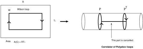
Figure 1: The correlator of Polyakov loops. The expectation value of a Wilson loop $W$ is equivalent to a correlator of the Polyakov loops $P$ and $P^{\dagger}$.

In the finite-temperature case, we must evaluate the correlator of Polyakov loops $P({\bf x})$. It can be evaluated in the same way as the Wilson loop, due to the following relation (as shown in Fig.1)

$$\langle\,P({\bf x})P^{\dagger}(0)\,\rangle_{\rm U(1)}=\langle\,W_{C}[A]\,\rangle_{\rm U(1)}.$$ (2.17)

Furthermore we can derive a Coulomb potential (at zero temperature) [19] or Yukawa-type potential (at finite temperature) using a hard thermal-loop (HTL) approximation [14] from a perturbative deformation part.

3 Topological Model and Two-dimensional Systems

3.1 Topological Model and Parisi-Sourlas Dimensional Reduction

The action of the topological model in four dimensions,

$$S_{\rm TQFT}[U,C,\bar{C},B]\;=\;\delta_{\rm B}\bar{\delta}_{\rm B}\int\!d^{4}x\,\left\{\frac{1}{2}\omega_{\mu}^{2}+iC\bar{C}\right\},$$ (3.1)

can be rewritten through the PS dimensional reduction [18] as

$$S_{\rm TQFT}[U] = \pi\int\!d^{2}x\,\omega_{\mu}^{2},\qquad\omega_{\mu}\equiv\frac{i}{g}U(x)\partial_{\mu}U(x)^{\dagger}$$ (3.2)

$$= \frac{\pi}{g^{2}}\int\!d^{2}x\,\partial_{\mu}U\,\partial_{\mu}U^{\dagger},$$

where we have omitted the ghost term. The above action (3.2) describes an $O(2)$ NLSM₂. Using $U(x)=\exp\{i\varphi(x)\}$ we obtain

$$S_{\rm TQFT}[\varphi]\;=\;\frac{\pi}{g^{2}}\int\!d^{2}x\,(\partial_{\mu}\varphi)^{2}.$$ (3.3)

If the $U(1)$ is not compact, then it becomes a free scalar field theory in two dimensions and has no topological object. Thus a confining phase cannot exist. If the $U(1)$ is compact, then it describes a periodic boson theory. The angle variable $\varphi(x)$ is periodic (mod $2\pi$), and so $\varphi(x)$ is a compact variable. It is well known that a compactness plays an important role in the confinement [2]. When we consider the system at finite (zero) temperature, the dimensionally reduced theory lives on the cylinder (plane). Let us consider the zero-temperature case. The solution of the classical field equation $\nabla^{2}\varphi(x)=0\;({\rm mod}~{}2\pi)$ is a harmonic function and hence $\varphi(x)$ is either constant or has singularities if we require that $\varphi(x)$ is constant at infinity. The solutions are called vortices and expressed by

$$\varphi(z)=\sum_{i=1}^{n}Q_{i}\,{\rm Im}\,\ln(z-z_{i}),~{}~{}~{}z\equiv x_{1}+i\,x_{0},$$ (3.4)

where $Q_{i}$ are the intensities of vortices and isolated singularities only are assumed. We can easily see that $\varphi(x)$ is a multi-valued function and varies by $2\pi$ as one turns a singularity anti-clockwise, but $\exp\{i\varphi(x)\}$ is well-defined everywhere, except at the singular points. The classical action for such a singular configuration is infinite, one can regularize the action by excluding a small region around each singularity (for example, a disk of radius $R_{0}$ centered on each singular point). Let $D$ be the remaining integration domain, we can obtain

$$S_{\rm vor}\left[\,(Q_{j},z_{j})\,\right] \equiv \frac{\beta^{\prime}}{2}\int_{D}d^{2}x\,(\partial_{\mu}\varphi)^{2},\quad\beta^{\prime}\equiv\frac{2\pi}{g^{2}}$$ (3.5)

$$= -\frac{8\pi^{3}}{g^{2}}\sum_{i<j}\,\frac{Q_{i}Q_{j}}{2\pi}\,\ln|z_{i}-z_{j}|\,+\,\sum_{i=1}^{n}Q_{i}^{2}\,\frac{2\pi^{2}}{g^{2}}\,\ln\frac{1}{R_{0}}.$$

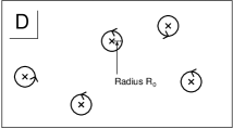
Figure 2: Vortices and integration domain $D$.

When we decompose the variable $\varphi$ as

$$\varphi\;=\;\varphi_{\rm vor}\,+\,\varphi_{\rm fluc}$$ (3.6)

where $\varphi_{\rm vor}$ is the vortex configuration and $\varphi_{\rm fluc}$ denotes the fluctuation around the classical configuration i.e., the spin wave, the action of an $O(2)$ NLSM₂ can be rewritten near a stationary configuration as

$$S_{\rm TQFT}=S[\,(Q_{i},z_{i})\,]+\frac{\beta^{\prime}}{2}\int\!d^{2}x(\partial_{\mu}\varphi_{\rm fluc})^{2},$$ (3.7)

and summing over all vortex sectors yields an approximate partition function

$$Z_{\rm TQFT}=Z_{\rm SW}\cdot Z_{\rm CG}.$$ (3.8)

The partition function of a CG system $Z_{\rm CG}$ is given by

$$Z_{\rm CG} = \sum_{n=0}^{\infty}\frac{\zeta^{2n}}{(n!)^{2}}\prod_{i=1}^{n}\int\frac{d^{2}x_{i}}{a^{2}}\frac{d^{2}y_{i}}{a^{2}}\,\exp\Bigg{[}-\frac{8\pi^{3}}{g^{2}}\,\Big{\{}\sum_{i<j}\left[\>\Delta(x_{i}-x_{j})+\Delta(y_{i}-y_{j})\right]$$ (3.9)

$$-\sum_{i,j}\,\Delta(x_{i}-y_{j})\,\Big{\}}\,\Bigg{]},$$

where the temperature of the CG system is

$$T_{\rm CG}\equiv\frac{g^{2}}{8\pi^{3}},$$ (3.10)

and $\Delta(x_{i}-x_{j})$ expresses the Coulomb potential on the plane,

$$\Delta(x-y)=-\frac{1}{2\pi}\ln\frac{|x-y|}{a}.$$ (3.11)

Here we have introduced the cut-off $a$ for the short-range interaction (length scale) through the change of variable $x_{i}\rightarrow x_{i}/a$ and

$$\zeta\equiv\exp\left[\frac{2\pi^{2}}{g^{2}}\,\ln\frac{R_{0}}{a}\right]\equiv\,\kappa^{2\pi^{2}/g^{2}},\quad\kappa\equiv\frac{R_{0}}{a},$$ (3.12)

plays a role of the chemical potential of the CG system and is determined by the value of $R_{0}$. The partition function of the spin wave $Z_{\rm SW}$ include no topological information and hence cannot contribute to the confinement in the gauge theory. Therefore we ignore this part hereafter. The CG system undergoes the BKT phase transition at certain temperature $1/8\pi$ as shown in Fig.3.

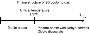
Figure 3: Two-dimensional Coulomb gas has two phases. Over the critical temperature $T_{\rm CG}=1/8\pi$, the system is in a plasma phase with Debye screening, and so the mass gap exists. Below $T_{\rm CG}$ it is in a dipole phase, in which Coulomb charges form dipoles. The system has a long range correlation and no mass gap.

In this case, the critical temperature $T_{\rm CG}=1/8\pi$ implies the critical coupling $g_{\rm cr}=\pi$ (see Appendix A for details). If $g<\pi$, then vortex and anti-vortex are tightly bound and a neutral pair of vortices tends to be formed. Thus the vortex effect can be ignored and hence the gauge theory is in the Coulomb phase. While, if $g>\pi$, then the CG system is in the plasma phase and hence the vortex effect exists. Therefore the linear potential between test charged particles is induced by vortices and the system is confined. The string tension can be obtained from the expectation value of the Wilson loop (for details, see Ref. [19]),

$$\langle\,W_{C}[A]\,\rangle_{\rm U(1)} = \langle\,W_{C}[V]\,\rangle_{\rm pU(1)}\,\langle\,W_{C}[\omega]\,\rangle_{\rm\scriptscriptstyle{TQFT}},$$

$$\langle\,W_{C}[\omega]\,\rangle_{\rm\scriptscriptstyle{TQFT}} \cong {\rm e}^{-\sigma_{\rm st}A(C)},$$ (3.13)

$$\sigma_{\rm st} = 4\pi^{2}\left(\frac{e}{g}\right)^{2}\zeta\Lambda^{2}\;=\;4\pi^{2}\left(\frac{e}{g}\right)^{2}\kappa^{2\pi^{2}/g^{2}}\,\Lambda^{2}$$ (3.14)

$$= 4\pi^{2}\left(\frac{e}{g}\right)^{2}\left[\frac{R_{0}}{a}\right]^{2\pi^{2}/g^{2}}\Lambda^{2}$$

where $A(C)=R\,T_{i},\,R=|{\bf x}|$ and $e$ is a charge of test particles. In particular, if the particles belong to the fundamental representation, $e=g/2$. Whether a confining string vanishes or not is determined by the phase of the CG system. Note that a string tension $\sigma_{\rm st}$ is proportional to $\zeta$. The $\zeta\rightarrow 0$ limit means $R_{0}\rightarrow 0$ and implies that the regularization of the action for the vortex configuration. Therefore the action tends to infinity and we fail to include the effect of vortices. As a result, a confining phase also disappears in the limit $\zeta\rightarrow 0$ as expected.

Comments on the relations between monopole in four dimensions and vortices in two-dimensions

From the viewpoint of the four-dimensional gauge theory, vortices in the two-dimensional $O(2)$ NLSM₂ would be interpreted as the point that the monopole world-line pieces the plane chosen when we use the PS mechanism as discussed in Refs. [10, 19]. (Concretely discussed in the $SU(2)$ case. The analogy holds in the $U(1)$ case.) In particular, a singularity (regularization) of an abelian monopole in the $U(1)$ theory should imply that of a vortex in the $O(2)$NLSM₂. It would be also expected that parameters $R_{0}$ and $a$ are a radius and a short-range cut-off for monopoles, respectively. The effect of monopoles which is relevant to the confinement of the system should be limited on the plane (area) enclosed by the Wilson loop, and we would be able to study the monopole effect effectively as vortex effect in the two-dimensional theory in our scenario through the PS mechanism. Technically, the gauge transformation $U(x)$ has the topological nature of the system or gauge group (i.e., monopole configuration), and we are considering the dynamics of this part in the two-dimensional theory through the PS dimensional reduction. Thus, we could consider the nature of the phase transition in the four-dimensional gauge theory as that of the CG system in the two-dimensional theory. One should consider that the phase transition from the viewpoint of four dimensions has a BKT-nature, which would be identical with that of the one-dimensional CG system.

3.2 Equivalence between Sine-Gordon model and Coulomb Gas System

The Euclidean action of the SG model on the plane (at zero temperature) or the cylinder (at finite temperature) is defined by

$$S_{\rm SG}[\phi]\;=\;\int\!d^{2}x\left\{\frac{1}{2}\left(\partial_{\mu}\phi\right)^{2}-\frac{m^{2}}{\bar{\lambda}}\left[\cos\left(\sqrt{\bar{\lambda}}\phi\right)-1\right]\right\}.$$ (3.15)

The above action contains two parameters $\bar{\lambda}\equiv\lambda/m^{2}$ and $m$. The $\bar{\lambda}$ is a dimensionless parameter but $m$ is dimensionful one. The partition function is given by

$$Z_{\rm SG} = \int[d\phi]\,\exp\left\{-S_{\rm SG}\right\}.$$ (3.16)

This can be rewritten as follows,

$$Z_{\rm SG} = \sum_{n=0}^{\infty}\frac{1}{n!}\left(\frac{m^{2}}{\bar{\lambda}}\right)^{n}\int[d\phi]\,{\rm e}^{-\int d^{2}x(1/2)\left(\partial_{\mu}\phi\right)^{2}}\left[\int\!d^{2}x\,\cos\left(\sqrt{\bar{\lambda}}\phi\right)\right]^{n}$$ (3.17)

$$= \sum_{n=0}^{\infty}\frac{1}{(2n)!}\left(\frac{m^{2}}{2\bar{\lambda}}\right)^{2n}\int[d\phi]\,{\rm e}^{-\int d^{2}x(1/2)\left(\partial_{\mu}\phi\right)^{2}}\left[\int\!d^{2}x\left\{{\rm e}^{i\sqrt{\bar{\lambda}}\phi}+{\rm e}^{-i\sqrt{\bar{\lambda}}\phi}\right\}\right]^{2n}$$

$$= \sum_{n=0}^{\infty}\frac{1}{(n!)^{2}}\left(\frac{m^{2}}{2\bar{\lambda}}\right)^{2n}\int[d\phi]\,{\rm e}^{-\int d^{2}x(1/2)\left(\partial_{\mu}\phi\right)^{2}}\prod_{j=1}^{2n}\int\!d^{2}x_{j}\,{\rm e}^{iq_{j}\phi(x_{j})}$$

$$= \sum_{n=0}^{\infty}\frac{1}{(n!)^{2}}\left(\frac{m^{2}}{2\bar{\lambda}}\right)^{2n}\left\langle\prod_{j=1}^{2n}\int d^{2}x_{j}\,{\rm e}^{iq_{j}\phi(x_{j})}\right\rangle,$$

where we have defined

$$q_{i}=\sqrt{\bar{\lambda}}\,\epsilon_{i}=\left\{\begin{array}[]{cc}\sqrt{\bar{\lambda}}&{\rm for}~{}1\leq i\leq n,\\ -\sqrt{\bar{\lambda}}&~{}~{}~{}~{}~{}~{}~{}~{}{\rm for}~{}n+1\leq i\leq 2n.\end{array}\right.$$ (3.18)

We have omitted the term $\exp\left[-(m^{2}/\bar{\lambda})\int d^{2}x\right]$ since it is canceled by the normalization of the partition function. Here we note that

$$\left\langle{\rm e}^{\int d^{2}x\,J\phi}\right\rangle \equiv \int[d\phi]\exp\left[\int\!d^{2}x\left(-\frac{1}{2}\left(\partial_{\mu}\phi\right)^{2}+J\phi\right)\right]$$ (3.19)

$$= \exp\left[\iint\!d^{2}xd^{2}y\,J(x)\Delta(x-y)J(y)\right],$$

where $\Delta(x-y)$ is a massless scalar field propagator,

$$\Delta(x-y)\;\equiv\;\int\!\frac{d^{2}p}{(2\pi)^{2}}\,\frac{{\rm e}^{ip\cdot(x-y)}}{p^{2}},$$ (3.20)

and this expression leads to Eq. (3.11) if we consider at zero temperature. In particular, if we choose an external field $J(x)$ as

$$J(x)\;=\;i\sum_{i=1}^{n}\,q_{i}\,\delta(x-x_{i}),$$ (3.21)

then we obtain

$$\left\langle\prod_{j=1}^{2n}{\rm e}^{iq_{j}\phi(x_{j})}\right\rangle\;=\;\left\{\begin{array}[]{cc}\exp\left[-(\bar{\lambda}/2)\sum_{j,k}^{~{}~{}}\epsilon_{j}\epsilon_{k}\Delta(x_{j}-x_{k})\right]&{\rm for}~{}\sum_{i=1}^{2n}\epsilon_{i}=0,\\ 0&{\rm for}~{}\sum_{i=1}^{2n}\epsilon_{i}\neq 0.\end{array}\right.$$ (3.22)

If the net charge is non-zero, then correlation functions vanish due to the translation symmetry under the following transformation

$$\phi(x)\;\longrightarrow\;\phi(x)\;+\;{\rm const}.$$

Using Eq. (3.19), we obtain the following partition function,

$$Z_{\rm SG}\! = \!\sum_{n=0}^{\infty}\frac{1}{(n!)^{2}}\left(\frac{m^{2}}{2\bar{\lambda}}\right)^{2n}\prod_{i=1}^{n}\int\!d^{2}x_{i}d^{2}y_{i}\,\exp\Bigg{[}-\bar{\lambda}\Big{\{}\sum_{i<j}[\Delta(x_{i}-x_{j})+\Delta(y_{i}-y_{j})]$$ (3.23)

$$-\sum_{i,j}\Delta(x_{i}-y_{j})\,\Big{\}}\,\Bigg{]},$$

where coordinates $x_{i},~{}(1\leq i\leq n)$ indicate positions of vortices and new coordinates $y_{i}\equiv x_{n+i},~{}(1\leq i\leq n)$ denote those of anti-vortices. Thus it has been shown that the SG model is equivalent to a neutral CG system whose temperature is defined by

$$T_{\rm CG}\,=\,\frac{1}{\bar{\lambda}}.$$ (3.24)

The phase transition in the SG model at the critical coupling $\bar{\lambda}=8\pi$ (often called the Coleman transition) corresponds to the BKT phase transition at the temperature $T_{\rm CG}=1/8\pi$ in terms of the CG system. One can identify two CG systems (3.9) and (3.23) through the following relations,

$$\frac{g^{2}}{8\pi^{3}}\,=\,\frac{1}{\bar{\lambda}}\quad(\mbox{temperature}),\qquad\frac{\zeta}{a^{2}}\,=\,\frac{m^{2}}{2\bar{\lambda}}\quad(\mbox{chemical potential}).$$ (3.25)

Thus, parameters of the SG model can be expressed by those of compact QED as

$$\bar{\lambda}\,=\,\frac{8\pi^{3}}{g^{2}},\qquad m\,=\,\frac{4\pi^{3/2}}{g}\,\zeta^{1/2}\Lambda,\qquad\Lambda\equiv\frac{1}{a}.$$ (3.26)

It should be noted that the length scale of the CG system, $a$ gives mass scale in the SG model. Recall that a string tension is $\sigma\,\propto\,\zeta$, and so vanishes as $\zeta\rightarrow 0~{}(R_{0}\rightarrow 0)$ and a confining phase disappears. The limit $\zeta\rightarrow 0$, which removes the regularization for singular vortices, means $m^{4}/\lambda\rightarrow 0$ and the SG model becomes free scalar field theory. That is, no kink solution exists. Kinks in the SG model are closely related to the existence of vortices in the CG system. Physically, this limit means that the fugacity of vortices (monopoles) becomes zero. Consequently, the effects of topological objects vanishes and hence a confining phase disappears. It is also commented that the variable $\varphi$ in an $O(2)$ NLSM₂ is related to $\phi$ in the SG model through

$$\partial_{\mu}\varphi\,=\,\frac{(2\pi)^{3/2}}{g}\,\epsilon_{\mu\nu}\partial_{\nu}\phi.$$ (3.27)

It is well known that the SG model is equivalent to the MT model. We shall summarize the relations between the CG system, SG and MT model in Fig. 4. It should be noted that the equivalence holds even in the finite-temperature case [25, 26].

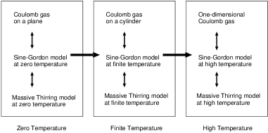
Figure 4: Relations between the CG system, SG model and MT model at zero and finite temperature.

We shall also list phase structures of these models on a plane in Tab. 1.

	Coulomb Gas	Sine-Gordon	Massive Thirring
	$T_{\rm CG}>1/8\pi$	$0<\bar{\lambda}<8\pi$	$g_{\rm\scriptscriptstyle{MT}}^{2}>-\pi/2$
Correlation Length	finite (Debye screening)	finite (mass scale)	finite (mass scale)
Phase	plasma	$\cos$ potential:	massive
	(vortices effect exists)	relevant	relevant
Renormalizability		super-renormalizable	super-renormalizable
Peculiar Point		$\bar{\lambda}=4\pi$	$g_{\rm\scriptscriptstyle{MT}}^{2}=0$
		free massive scalar†	free massive fermion
Transition Point	$T_{\rm CG}=1/8\pi$	$\bar{\lambda}=8\pi$	$g_{\rm\scriptscriptstyle{MT}}^{2}=-\pi/2$
		$\cos$ potential:
		marginally irrelevant	marginally irrelevant
Renormalizability		renormalizable	renormalizable
	$T_{\rm CG}<1/8\pi$	$\bar{\lambda}>8\pi$	$g_{\rm\scriptscriptstyle{MT}}^{2}<-\pi/2$
Correlation Length	infinite (no screening)	infinite	infinite
		no quantum ground state
Phase	molecule	$\cos$ potential:	massless
	(no vortex effect)	irrelevant	irrelevant
Renormalizability		not renormalizable	not renormalizable

^†: Additional renormalization is needed.

Table 1: Phases of the Coulomb gas system, sine-Gordon and massive Thirring model.

Confining Phase Transition from the viewpoint of the Renormalization Group

From the perturbed conformal field theory (CFT) point of view, the SG model can be considered as a perturbation of the free massless two-dimensional scalar field theory by the relevant conformal operators $\exp(\pm i\sqrt{\bar{\lambda}}\phi)$ whose scale dimensions

$$\Delta_{\rm SG}=\frac{\bar{\lambda}}{8\pi}=\frac{p}{p+1},$$ (3.28)

where we have introduced a real parameter $p$ defined by

$$p\equiv\frac{\bar{\lambda}}{8\pi-\bar{\lambda}}.$$ (3.29)

In fact, if we take $0\leq\sqrt{\bar{\lambda}}\leq\sqrt{8\pi}$, then there is a family of CFTs depending on one parameter $p$. The corresponding mass parameter $m^{2}$ has a complementary dimension,

$$m^{2}\,\sim\,[{\rm mass}]^{2/(p+1)}=[{\rm mass}]^{(8\pi-\bar{\lambda})/4\pi}.$$ (3.30)

Thus we can read off the behavior of a cosine potential for each value of $\bar{\lambda}$. It is relevant for $0\leq\bar{\lambda}<8\pi$, marginal for $\bar{\lambda}=8\pi$, and irrelevant for $\bar{\lambda}>8\pi$.

3.3 Gauge Theory and Massive Thirring Model

The action of the MT model in the two-dimensional Euclidean space with metric $(+,+)$, is given by

$$S_{\rm MT}[\psi,\bar{\psi}]\;=\;\int\!d^{2}x\,\left\{-\bar{\psi}(\gamma^{\mu}\partial_{\mu}+m_{\rm\scriptscriptstyle{MT}})\psi+\frac{1}{2}g_{\rm\scriptscriptstyle{MT}}^{2}\bar{\psi}\gamma_{\mu}\psi\bar{\psi}\gamma^{\mu}\psi\right\}.$$ (3.31)

The Euclidean gamma matrices (following the notation in Ref. [23]) are defined by

$$\gamma^{1}\,=\,\sigma_{1}\,=\,\begin{pmatrix}0&1\\ 1&0\end{pmatrix},\quad\gamma^{2}\,=\,\sigma_{2}\,=\,\begin{pmatrix}0&-i\\ i&0\end{pmatrix},\quad\gamma^{5}\,=\,-i\sigma_{1}\sigma_{2}\,=\,\sigma_{3}\,=\,\begin{pmatrix}1&0\\ 0&-1\end{pmatrix},$$

and obeys the standard relations

$$\gamma^{\mu}\gamma^{\nu}\,+\,\gamma^{\nu}\gamma^{\mu}\,=\,2\delta^{\mu\nu}, \gamma^{\mu}\gamma^{5}\,+\,\gamma^{5}\gamma^{\mu}\,=\,0,$$

$$\gamma^{\mu}\gamma^{\nu}\,=\,\delta^{\mu\nu}\,+\,i\epsilon^{\mu\nu}\gamma^{5}, \gamma^{\mu}\gamma^{5}\,=\,-i\epsilon^{\mu\nu}\gamma^{\nu},$$

are satisfied. The anti-symmetric tensor $\epsilon_{\mu\nu}$ is defined by $\epsilon_{12}=-\epsilon_{21}=1,\;\epsilon^{12}=-\epsilon^{21}=1$. It has been well known that the SG/MT duality holds at zero temperature [24] and finite temperature [25, 26] if the following relations

$$\frac{4\pi}{\bar{\lambda}}\,=\,1+\frac{g_{\rm\scriptscriptstyle{MT}}^{2}}{\pi},\qquad\frac{m^{2}}{\bar{\lambda}}\,=\,\rho\,m_{\rm\scriptscriptstyle{MT}},$$ (3.32)

are satisfied. Here $\rho$ and $m_{\rm\scriptscriptstyle{MT}}$ are a renormalization scale and a renormalized mass at that scale, respectively. Hereafter, we shall set $\rho=m_{\rm\scriptscriptstyle{MT}}$. The condition (3.32) can be rewritten as

$$m_{\rm\scriptscriptstyle{MT}}\,=\,\frac{m}{\sqrt{\bar{\lambda}}},\qquad g_{\rm\scriptscriptstyle{MT}}^{2}\,=\,\frac{4\pi^{2}}{\bar{\lambda}}-\pi.$$ (3.33)

If a coupling constant of the SG model $\bar{\lambda}\equiv\lambda/m^{2}$ becomes $4\pi$, then a mass of the MT model becomes zero. Thus $\bar{\lambda}=4\pi$ corresponds to a massless Thirring model. Combining Eq.  (3.33) with Eq. (3.26), we can obtain the relations between each parameter of the MT model and gauge theory as

$$m_{\rm\scriptscriptstyle{MT}}\,=\,\sqrt{2\zeta}\Lambda,\qquad g_{\rm\scriptscriptstyle{MT}}^{2}\,=\,\frac{g^{2}}{2\pi}-\pi.$$ (3.34)

Here, note that $m_{\rm\scriptscriptstyle{MT}}$ vanishes in the limit of $\zeta\rightarrow 0~{}(R_{0}\rightarrow 0)$. That is, the MT model becomes a massless Thirring model. This fact is consistent to that a cosine potential of the SG model also vanishes as $\zeta\rightarrow 0$ since a mass perturbation in the MT model corresponds to a cosine potential perturbation in the SG model. Also, the current and mass equivalence, respectively,

$$\bar{\psi}\gamma_{\mu}\psi = \frac{\sqrt{\bar{\lambda}}}{2\pi}\,\epsilon_{\mu\nu}\partial_{\nu}\phi,$$ (3.35)

$$m_{\rm\scriptscriptstyle{MT}}\,\bar{\psi}\psi = \frac{m^{2}}{\bar{\lambda}}\cos\left(\sqrt{\bar{\lambda}}\phi\right),$$ (3.36)

are also useful in discussing the relations between topological charges, such as a monopole charge in the gauge theory, vortex intensity in the $O(2)$ NLSM₂, kink number in the SG model and fermion number in the MT model. In particular, Eq. (3.35) means the equivalence between a kink number and fermion number. We can again understand a mass term in the MT model from the viewpoint of the perturbed CFT. Recall that a cosine potential in the SG model is a perturbation from a massless free scalar theory. A mass term in the action of the MT model corresponds to a cosine potential through the abelian bosonization, and we can identify a mass term in the MT model as a perturbation from a massless Thirring model. Correspondingly, the monopole effect realized by a cosine potential in the SG model is described by a mass term in the MT model. Such a correspondence leads us to expect the relation between the monopole condensate in compact QED and fermion one in the MT model.

Relations of Some Quantities

	Gauge	$O(2)$ NLSM2	SG model	MT model
Variable	$A_{\mu}=V_{\mu}+\omega_{\mu}$	$U={\rm e}^{i\varphi}$	$\phi$	$\psi$
Topological Objects	monopoles	vortices	kinks	fermions
Topological Charge	magnetic charge	intensity	kink number	fermion number
				$U(1)_{V}$
Global Symmetry	${\rm e}^{i\alpha}\in U(1)$	$\varphi\rightarrow\varphi+2\pi n$	$\phi\rightarrow\phi+\frac{2\pi}{\sqrt{\bar{\lambda}}}n$	$\psi\rightarrow{\rm e}^{2\pi n\gamma^{5}}\psi$
(Residual)	global $U(1)$	${}^{\forall}n\in\mathbb{Z}$	${}^{\forall}n\in\mathbb{Z}$	${}^{\forall}n\in\mathbb{Z}$
Broken Symmetry		$\varphi\rightarrow\varphi+\alpha$	$\phi\rightarrow\phi+\frac{1}{\sqrt{\bar{\lambda}}}a$	$\psi\rightarrow{\rm e}^{ia\gamma^{5}}\psi$
by Topological Objects		${}^{\forall}{\rm e}^{i\alpha}\in U(1)$	${}^{\forall}a\in\mathbb{R}$	${}^{\forall}{\rm e}^{ia\gamma^{5}}\in U(1)_{A}$
Scale Parameters	$\Lambda\equiv 1/a$ UV cut-off†1 $R_{0}$ monopole radius	$a$ length scale†2 $R_{0}$ vortex radius	$m=\frac{4\pi^{3/2}}{g}\zeta^{1/2}\Lambda$ mass	$m_{\rm\scriptscriptstyle{MT}}=\sqrt{2\zeta}\Lambda$ fermion mass
Characteristic Parameter	$g,\,a,\,R_{0}$	$\zeta,\,a,\,R_{0}$	$m,\,\bar{\lambda}$	$m_{\rm\scriptscriptstyle{MT}},\,g_{\rm\scriptscriptstyle{MT}}$
Source	$\partial_{\mu}\omega_{\nu}$	$\frac{1}{g}\partial_{\mu}\varphi$	$\frac{\sqrt{\bar{\lambda}}}{2\pi}\epsilon_{\mu\nu}\partial_{\nu}\phi$	$j_{\mu}\equiv\bar{\psi}\gamma_{\mu}\psi$
	magnetic source		kink number	vector current
(Dual)	$\epsilon_{\mu\nu\rho\sigma}\partial_{\rho}\omega_{\sigma}$	$\frac{1}{g}\epsilon_{\mu\nu}\partial_{\nu}\varphi$	$\frac{\sqrt{\bar{\lambda}}}{2\pi}\partial_{\mu}\phi$	$j_{5\mu}\equiv\bar{\psi}\gamma_{\mu}\gamma_{5}\psi$
Source	electric source			axial current
If non-compact	no monopole	no vortex	free boson	massless fermion

$\dagger 1$, $\dagger 2$ : The parameter $a$ denotes short-range cut-off for interaction between monopoles or vortices, respectively.

Table 2: Relations of some quantities.

We shall briefly remark that some quantities such as currents, topological objects and these charges are closely related. Using Eq. (3.27) and Eq. (3.35) leads to the current relation,

$$\omega_{\mu} = \frac{1}{g}\partial_{\mu}\varphi\quad\mbox{($O(2)$ NLSM${}_{2}$)}$$ (3.37)

$$= \left(\frac{2\pi}{g}\right)\frac{\sqrt{\bar{\lambda}}}{2\pi}\epsilon_{\mu\nu}\partial_{\nu}\phi\quad\mbox{(SG model)}$$

$$= \left(\frac{2\pi}{g}\right)\bar{\psi}\gamma_{\mu}\psi\equiv\left(\frac{2\pi}{g}\right)j_{\mu}\quad\mbox{(MT model)}.$$

From Eq. (3.37) we can show a relation of topological charges through the integral along the closed loop $C$,

$$\oint_{C}\omega_{\mu}dx^{\mu} = \frac{1}{g}\oint\partial_{\mu}\varphi\,dx^{\mu}\,=\,\sum_{i}\,\frac{2\pi}{g}\,Q_{i}.$$ (3.38)

In particular, the magnetic charge of monopoles (or intensity of vortices) implies a mass $m_{\rm\scriptscriptstyle{MT}}$ in the MT model. From the identity

$$\oint_{C}\omega_{\mu}dx^{\mu}\,=\int_{S}\!d^{2}x\,\epsilon_{\mu\nu}\,\partial_{\mu}\omega_{\nu}$$ (3.39)

$$= \frac{2\pi}{g}\int_{S}\!d^{2}x\,\partial_{\mu}(\epsilon_{\mu\nu}\bar{\psi}\gamma_{\nu}\psi)=\frac{2\pi}{g}\int_{S}\!d^{2}x\,\partial_{\mu}(i\bar{\psi}\gamma_{\mu}\gamma_{5}\psi),$$

the non-zero flux of magnetic monopoles (non-zero topological charge) means that the axial current $j_{5\mu}\equiv\bar{\psi}\gamma_{\mu}\gamma_{5}\psi$ does not conserve classically. That is, a magnetic flux breaks the chiral symmetry of the MT model at the classical level. This result agrees with the fact that a mass of the MT model is proportional to $\zeta$. If there is no topological effect, then $\zeta$ vanishes and a mass of the MT model becomes zero (i.e., a massless Thirring model) where the current $j_{5\mu}$ is conserved classically. Finally, we shall summarize the above results and list the relationship between some quantities of compact QED, $O(2)$ NLSM₂, SG model and MT model in Tab. 2.

4 Coulomb Gas Behavior and Phase Structure

First, we shall briefly review phase structures of the one-dimensional CG and MT model shown in Ref. [21]. In particular, a phase structure of the MT model in the high-temperature region can be investigated by using exact results in a one-dimensional CG system [27]. Next, we will derive the thermal pressure of the topological model from these results. Thus we can decide a phase structure in terms of a one-dimensional CG system. Finally, we will estimate the critical-line equation of the gauge theory and comment on the nature and order of the phase transition.

4.1 Phase Structure of One-dimensional Coulomb Gas

A one-dimensional CG is an exactly-solvable model and some quantities can be exactly calculated. In particular, the thermal pressure in the one-dimensional CG system is very useful and powerful for investigating a phase structure of the MT model. A one-dimensional CG system, which consists of $N$ positive charged particles and $N$ negative ones, is described by the following partition function,

$$Z_{\rm 1CG}(z,\theta,\sigma,L)\,=\,\sum_{N=0}^{\infty}\frac{z^{2N}}{(N!)^{2}}\,\prod_{i=1}^{2N}\int_{0}^{L}\!\!dq_{i}\,\exp\left[\frac{2\pi\sigma^{2}}{\theta}\!\!\!\!\sum_{1\leq i<j\leq 2N}\!\!\!\!\epsilon_{i}\epsilon_{j}\,|q_{i}-q_{j}|\right],$$ (4.1)

where $\theta$ and $L$ are temperature and size of the system, respectively and $\epsilon_{i}=1$ for $i\leq N$ and $\epsilon_{i}=-1$ for $i\geq N+1$. The magnitude of the charge is denoted by $\sigma$. The fugacity $z$ is related to the chemical potential $\mu_{\rm\scriptscriptstyle{CG}}$ through

$$z=\sqrt{2\pi M\theta}\,\exp\left(\frac{\mu_{\rm\scriptscriptstyle{CG}}}{\theta}\right),$$ (4.2)

where $M$ is a mass of particles. In the thermodynamic limit $L\rightarrow\infty$, the thermal pressure $P(z,\theta,\sigma)$ and the mean particle density $n(z,\theta,\sigma)$ are defined by

$$P(z,\theta,\sigma)\;=\;\lim_{L\rightarrow\infty}\,\frac{\theta}{L}\ln Z_{\rm 1CG}(z,\theta,\sigma,L),$$ (4.3)

$$n(z,\theta,\sigma)\;=\;\frac{z}{\theta}\,\frac{\partial}{\partial z}P(z,\theta,\sigma).$$ (4.4)

The thermal pressure of a one-dimensional CG can be exactly calculated and is given by

$$P(z,\theta,\sigma)\;=\;2\pi\sigma^{2}\gamma_{0}(\hat{z}),~{}~{}~{}~{}\hat{z}\equiv\frac{z\,\theta}{2\pi\sigma^{2}},$$ (4.5)

where $\gamma_{0}(\hat{z})$ is the highest eigenvalue of the Mathieu’s differential equation

$$\left[\frac{d^{2}}{d\phi^{2}}+2\hat{z}\cos\phi\right]\,y(\phi)=\gamma\,y(\phi)$$ (4.6)

with $y(\phi+2\pi)=y(\phi)$. The eigenvalues and eigenfunctions of Eq. (4.6) are well known and can be calculated by Mathematica. Remark that asymptotic forms of $\gamma_{0}(\hat{z})$ for sufficiently large and small $\hat{z}$ becomes as follows:

$$\gamma_{0}(\hat{z})\;\simeq\;2\hat{z}^{2}\,+\,O(\hat{z}^{4}),~{}~{}~{}~{}{\rm for}~{}~{}\hat{z}\ll 1,$$ (4.7)

$$\gamma_{0}(\hat{z})\;\simeq\;2\hat{z}-\sqrt{\hat{z}}\,+\,O(1),~{}~{}~{}{\rm for}~{}~{}\hat{z}\gg 1.$$ (4.8)

That is, if $\hat{z}$ is small, it behaves as a quadratic curve. Since $\gamma_{0}(\hat{z})$ is a monotonous function rapidly increasing like an exponential function, the most important parameter determining phases of a one-dimensional CG is $\hat{z}$, which plays a role as a certain order parameter. We have summarized in Tab. 3 the relationship between the value of $\hat{z}$, thermal pressure and phases of the CG system.

$\hat{z}$	Pressure	1D Coulomb gas
Small	Small	Molecule Phase
Large	Large	Plasma Phase

Table 3: The parameter $\hat{z}$, thermal pressure and phases of the one-dimensional CG system.

4.2 Phase Structure of Massive Thirring Model

In the high-temperature regime, using the partition function of the one-dimensional CG, $Z_{\rm 1CG}(z,\theta,\sigma,L)$, we can write the partition function of the MT model, $Z_{\rm MT}(T,L)$ as

$$Z_{\rm MT}(T,L)=Z_{0}^{F}(T,L)\cdot Z_{\rm 1CG}(z,\theta,\sigma,L),$$ (4.9)

where $z,\,\theta$ and $\sigma$ are defined by

$$z\,\equiv\,\frac{m_{\rm\scriptscriptstyle{MT}}^{2}}{2T}\left(\frac{2T}{m_{\rm\scriptscriptstyle{MT}}}\right)^{(1+g_{\rm\scriptscriptstyle{MT}}^{2}/\pi)^{-1}}\!\!\!\!\!\!\!\!\!\!\!,\quad\theta\,\equiv\,T,\quad\sigma\,\equiv\,T\sqrt{\frac{\pi}{\pi+g_{\rm\scriptscriptstyle{MT}}^{2}}},$$ (4.10)

and $Z_{0}^{F}(T,L)$ is the partition function for a two-dimensional free massless Fermi gas defined by

$$Z_{0}^{F}(T,L)\equiv\exp\left(\frac{\pi LT}{6}\right).$$ (4.11)

Here we have ignored irrelevant vacuum terms. Parameters of a one-dimensional CG system $z,\theta$ and $\sigma$ is expressed by those of the MT model. The partition function (4.9) leads to the thermal pressure of the MT model,

$$P_{\rm MT}(T)\,=\,\frac{\pi}{6}T^{2}+P_{\rm 1CG}(T,g_{\rm\scriptscriptstyle{MT}},m_{\rm\scriptscriptstyle{MT}}).$$ (4.12)

The thermal pressure induced by particles forming a one-dimensional CG system, $P_{\rm 1CG}$ can be expressed by parameters of the MT model as

$$P_{\rm 1CG}(T,g_{\rm\scriptscriptstyle{MT}},m_{\rm\scriptscriptstyle{MT}}) = \frac{2\pi T^{2}}{1+g_{\rm\scriptscriptstyle{MT}}^{2}/\pi}\,\gamma_{0}(\hat{z}),$$

$$\hat{z} \equiv \frac{m_{\rm\scriptscriptstyle{MT}}^{2}}{4\pi T^{2}}\left(1+\frac{g_{\rm\scriptscriptstyle{MT}}^{2}}{\pi}\right)\left(\frac{2T}{m_{\rm\scriptscriptstyle{MT}}}\right)^{(1+g_{\rm\scriptscriptstyle{MT}}^{2}/\pi)^{-1}}.$$ (4.13)

The numerical plot of $\hat{z}$ as a function of $T/m_{\rm\scriptscriptstyle{MT}}$ and $g_{\rm\scriptscriptstyle{MT}}^{2}/\pi$ is shown in Fig. 5.

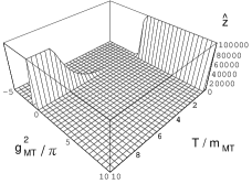
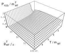
Fig. 5 (a) Fig. 5 (b)

Figure 5: The behavior of $\hat{z}$ and thermal pressure $P_{\rm 1CG}/m^{2}_{\rm\scriptscriptstyle{MT}}$.

A cliff and slope appear in Fig. 5 (a). These mean that the thermal pressure is very strong, and hence a one-dimensional CG system is in a plasma phase. There exists a slope in the negative-coupling and high-temperature regime but we cannot believe this result since it is out of the DR regime [21],

$$T\gg m_{\rm\scriptscriptstyle{MT}},\quad g_{\rm\scriptscriptstyle{MT}}^{2}>0,$$ (4.14)

$$T\gtrsim m_{\rm\scriptscriptstyle{MT}},\quad g_{\rm\scriptscriptstyle{MT}}^{2}/\pi\gg 1,$$ (4.15)

where the expression of the thermal pressure (4.12) is reliable. The constraints for the temperature imply the region where the dimensional reduction (a one-dimensional CG approximation) is valid. Those for the coupling ensure the existence of the thermo-dynamical limit. It should be remarked that the first term in Eq. (4.12) implies the finite-size effect of the cylinder (i.e., geometrical force) as discussed in Appendix B, and hence it does not depend on parameters of the MT model and universal. Thus we will omit this term in studying the phase structure since it is purely geometrical contribution. In the three specific regions of the MT model, the behavior of a one-dimensional CG system has been analytically investigated [21], and we shall list results of Ref. [21] below for the purpose of studying compact QED.

1. $g_{\rm\scriptscriptstyle{MT}}^{2}\,\gg\,\pi$ and $T\,\gg\,m_{\rm\scriptscriptstyle{MT}}g_{\rm\scriptscriptstyle{MT}}/2\pi$: Then, $\hat{z}\ll 1$, and the thermal pressure becomes as

   $$\frac{P_{\rm 1CG}}{m^{2}_{\rm\scriptscriptstyle{MT}}}\;\sim\;\left(\frac{m_{\rm\scriptscriptstyle{MT}}g_{\rm\scriptscriptstyle{MT}}}{2\pi T}\right)^{2}\;\ll\;1.$$ (4.16)

   Thus the thermal pressure vanishes as $T\rightarrow\infty$ and hence the system is in the “molecule” phase.

2. $g_{\rm\scriptscriptstyle{MT}}^{2}\,\gg\,\pi$ and $T\,\ll\,m_{\rm\scriptscriptstyle{MT}}g_{\rm\scriptscriptstyle{MT}}/2\pi$: In this region, $\hat{z}\gg 1$ and the thermal pressure behaves as

   $$\frac{P_{\rm 1CG}}{m_{\rm\scriptscriptstyle{MT}}^{2}}\;\sim\;1-\frac{\pi T}{m_{\rm\scriptscriptstyle{MT}}g_{\rm\scriptscriptstyle{MT}}}\;\gg\;\frac{1}{2}.$$ (4.17)

   Thus, the system is in the “plasma” phase.

3. $0\,<\,g_{\rm\scriptscriptstyle{MT}}^{2}\,\ll\,1$ and $T\,\gg\,m_{\rm\scriptscriptstyle{MT}}/2\pi$: We have $\hat{z}\,\simeq\,m_{\rm\scriptscriptstyle{MT}}/2\pi T$, which leads to $\hat{z}\ll 1$. Thus the system is in the “molecule” phase and the thermal pressure behaves as

   $$\frac{P_{\rm 1CG}}{m^{2}_{\rm\scriptscriptstyle{MT}}}\;\sim\;\frac{1}{\pi}.$$ (4.18)

4.3 Phase Structure of Compact QED

We can translate previous results of the CG system (MT model) into compact QED. By the use of Eq. (3.34), we can rewrite the thermal pressure and its argument of the one-dimensional CG system (MT model) in terms of compact QED as follows:

$$P_{\rm 1CG}(T,g,\Lambda,\kappa)\;=\;\frac{4\pi^{3}T^{2}}{g^{2}}\,\gamma_{0}(\hat{z}),$$ (4.19)

$$\hat{z}\;=\;\frac{g^{2}}{2\pi^{3}}\left(\frac{2T^{2}}{\zeta\Lambda^{2}}\right)^{(\pi^{2}-g^{2})/g^{2}}\,=\,\frac{g^{2}}{2\pi^{3}}\left(\frac{2T^{2}}{\Lambda^{2}}\right)^{(\pi^{2}-g^{2})/g^{2}}\kappa^{2\pi^{2}(g^{2}-\pi^{2})/g^{4}}.$$ (4.20)

We have numerically plotted $\hat{z}$ and thermal pressure $P_{\rm 1CG}/\Lambda^{2}$ as functions of $T$ and $g$ at fixed $\Lambda$ and $\kappa$ in Fig. 6. It can be easily seen that the theory with strong coupling is confined. That is, a confining phase similar to the lattice gauge theory appears in the strong-coupling regime. Non-trivial phase structure tends to disappear as $\kappa$ becomes small.

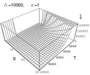
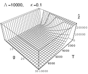
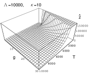
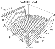
Fig. 6 (a) Fig. 6 (b) Fig. 6 (c) Fig. 6 (d)

Figure 6: The plot of $\hat{z}$ is shown in Figs. 6 (a), (b) and (c) at fixed $\Lambda=10000$, and $\kappa=1,\,0.1$ and $10$, respectively. In Fig. 6 (d), the dimensionless quantity $P_{\rm 1CG}/\Lambda^{2}$ is plotted.

Here, we should remember the validity of our calculations. Recall that we have used the one-dimensional CG approximation and equivalence between a one-dimensional CG and high-temperature MT model in our derivation. The validity of the approximation and equivalence is restricted within the DR regime where the existence of the thermo-dynamical limit is also guaranteed. This regime of compact QED is expressed by

$$T\gg\sqrt{2}\,\kappa^{\pi^{2}/g^{2}}\Lambda,\quad g^{2}>2\pi^{2},$$ (4.21)

$$T\gtrsim\sqrt{2}\,\kappa^{\pi^{2}/g^{2}}\Lambda,\quad g^{2}\gg 4\pi^{2}.$$ (4.22)

The constraints for the coupling are obstacles to propose the existence of another confining phase. As discussed in Ref. [21], we might formally take the gauge-coupling $g$ arbitrary from the viewpoint of the CG system, although extra renormalizations at least would be required from the standpoint of the MT model. Also, compact QED would possibly have the same renormalization problem as in the MT model. In addition, it is quite well known that the density of magnetic monopoles decreases rapidly as the coupling constant gets smaller [3]. That is, monopole effects would almost vanish in the weak-coupling region. Thus we conclude and strongly remark that the confinement at weak-coupling and high-temperature would not appear. We can also estimate the critical temperature as a function of $g$ at fixed values of $\Lambda,\,\mu$ and $\kappa$ by setting $\hat{z}\equiv l~{}({\rm const})$. The critical-line equation can be evaluated by

$$T_{\rm cr} = \frac{\zeta^{1/2}\Lambda}{\sqrt{2}}\left(\frac{2\pi^{3}l}{g^{2}}\right)^{g^{2}/2(\pi^{2}-g^{2})}$$ (4.23)

$$= \frac{\Lambda}{\sqrt{2}}\,\kappa^{\pi^{2}/g^{2}}\left(\frac{2\pi^{3}l}{g^{2}}\right)^{g^{2}/2(\pi^{2}-g^{2})}.$$

The critical temperature (4.23) is numerically plotted in Fig. 7.

Fig. 7 (a) Fig. 7 (b) Fig. 7 (c)

Figure 7: Critical-line equations: In Figs. 7 (a), (b) and (c) the critical-lines for $l=1$ are plotted at fixed values.

In particular, in the strong-coupling region, we can obtain from Eq. (4.23) the asymptotic line,

$$T_{\rm cr}^{\rm asy}\;\simeq\;\frac{\Lambda\,\kappa^{\pi^{2}/g^{2}}}{2\pi^{3/2}l^{1/2}}\,g,$$ (4.24)

where if we take $l=1/16$, Eq. (4.24) is precisely identical with the asymptotic line given by a perturbative method in our previous work [15]. A one-dimensional CG approximation does not depend on a perturbation theory in the two-dimensional theory, and hence this result is non-trivial and further confirms the validity of our previous result for the asymptotics of the critical-line equation at sufficiently high-temperature and strong-coupling region of compact QED. In conclusion, the phase structure shown in Fig. 8 is obtained, and agrees with our previous results [14, 15]. Moreover, we can analytically investigate the specific three regime denoted in subsection 4.2. The results are listed below.

1. $g^{2}\,\gg\,4\pi^{2},~{}~{}T\,\gg\,T_{{\rm cr}\,(l=1)}^{\rm asy}\,$: In this region, $\hat{z}\,\ll\,1$ and

   $$P_{\rm 1CG}\;\sim\;\frac{\Lambda^{4}g^{2}}{2\pi^{3}T^{2}}\,\kappa^{4\pi^{2}/g^{2}}\!\gg\,2\Lambda^{2}\,\kappa^{2\pi^{2}/g^{2}}.$$

   Thus a one-dimensional CG is in the “molecule” phase and hence compact QED is in a deconfining phase (Coulomb phase).

2. $g^{2}\,\gg\,4\pi^{2},~{}~{}T\,\ll\,T_{{\rm cr}\,(l=1)}^{\rm asy}\,$: Now $\hat{z}\,\gg\,1$ and

   $$P_{\rm 1CG}\;\sim\;2\Lambda^{2}\,\kappa^{2\pi^{2}/g^{2}}\!-\,\frac{2\pi^{3/2}\Lambda T}{g}\,\kappa^{\pi^{2}/g^{2}}\!\ll\,\Lambda^{2}\,\kappa^{2\pi^{2}/g^{2}}.$$

   Thus a one-dimensional CG is in the “plasma” phase, and so the gauge theory is confined. Of course, this result also agrees with our previous result.

3. $2\pi^{2}\,<\,g^{2}\ll 2\pi^{2}+2\pi,~{}~{}T\,\gg\,(\Lambda/\sqrt{2}\pi)\,\kappa^{\pi^{2}/g^{2}}\,$: In this region, $\hat{z}\,\ll\,1$ and

   $$P_{\rm 1CG}\;\sim\;\frac{2\Lambda^{2}}{\pi}\,\kappa^{2\pi^{2}/g^{2}}.$$

   Thus a one-dimensional CG is in the “molecule” phase, and hence the gauge theory should be in the Coulomb phase. This result has also no contradiction.

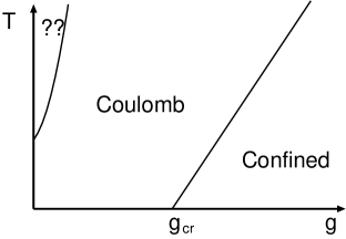
Figure 8: Phase diagram of a compact $U(1)$ gauge theory.

It should be remarked that the critical-line equation derived in our previous work [15] appears in the region I, II.

Comments on the Order of the Confining Transition

In general, a photon mass is taken as the order-parameter [1] of the confinement in compact QED. The confining transition of the four-dimensional compact QED is second-order if it is second-order at zero temperature [1, 8]. If it is first-order at zero temperature, then the tri-critical point exists on the critical-line as shown in Fig. 9.

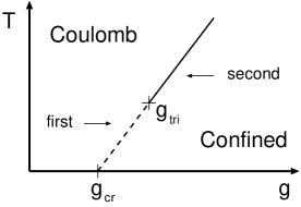
Figure 9: The order of the confining-deconfining phase transition. If the order is first at zero temperature, then the tri-critical point exists.

Several numerical simulation results of the compact $U(1)$ lattice gauge theory have been reported until now. However, some of them claim that it is first-order, and others show that it is second. It seems rather difficult to decide the order numerically in the lattice formulation. It is because we have a continuum-limit problem as noted in Introduction. Our scenario is based on the continuum formulation and it would be possible to avoid such a problem. However, in our scenario, we can only guess the nature of the phase transition is BKT-type and still have no clear answer. The photon mass cannot be calculated yet. This is one of the most interesting future problems.

5 Fermion Condensate versus Monopole Condensate

In this section we will discuss the correspondence between fermion condensate in the MT model and monopole condensate in compact QED. In particular, the chiral operators of the MT model correspond to the monopoles and anti-monopoles in compact QED. Again, the exact results of the one-dimensional CG system are utilized. It can be also seen that the confining phase transition in compact QED is closely related to the chiral symmetry restoration in the MT model. This relation seems natural from the viewpoint of the perturbed CFT.

5.1 Fermion Condensate and Chiral Symmetry in Massive Thirring Model

We will review the equivalence between the chiral symmetry restoration in the MT model and the behavior of the one-dimensional CG system [21]. The charged particles consisting of the CG system could be interpreted as monopoles and anti-monopoles in compact QED. Thus the chiral symmetry in the MT model is intimately related to the behavior of monopoles in compact QED. In particular, the fermion condensate corresponds to the monopole condensate. In the DR regime, utilizing the exact results for the one-dimensional CG system, the fermion condensate in the MT model can be calculated as

$$\langle\langle\bar{\psi}\psi\rangle\rangle\;=\;\frac{\partial}{\partial\,m_{\rm MT}}P_{\rm MT}(T).$$ (5.1)

We now consider the system coupled with the thermal bath and so the vacuum expectation value is replaced with the thermal expectation value $\langle\langle\;\ldots\;\rangle\rangle$ defined by

$$\langle\langle\;\ldots\;\rangle\rangle\equiv\frac{1}{Z(T)}{\rm Tr}\left(\;\ldots\;{\rm e}^{-\beta\hat{H}}\right)\,=\,\frac{N_{\beta}}{Z(T)}\int_{\rm anti-periodic}\!\!\!\!\!\!\!\!\!\!\!\!\!\!\!\!\!\!\!\![d\psi][d\bar{\psi}]\;\ldots\;\exp(-S[\psi,\bar{\psi}]),$$ (5.2)

where $N_{\beta}$ is an infinite $T$-dependent constant arising in the path-integral description. Here, we shall introduce the one-charge density functions $f_{\pm}(z,\theta,\sigma,L;X)$ defined by

$$f_{+}(z,\theta,\sigma,L;X)$$

$$= \frac{1}{Z_{\rm 1CG}}\sum_{N=1}^{\infty}\frac{z^{2N}}{(N!)^{2}}\left(\prod_{i=1}^{2N}\int_{0}^{L}\!\!dx_{i}\right)\sum_{j=1}^{N}\delta(x_{j}-X)\exp\left[\frac{2\pi\sigma^{2}}{\theta}\!\!\!\!\!\sum_{1\leq j<i\leq 2N}\!\!\!\!\epsilon_{i}\epsilon_{j}|x_{i}-x_{j}|\right]$$

$$= \frac{1}{Z_{\rm 1CG}}\sum_{N=1}^{\infty}\frac{z^{2N}}{N!(N-1)!}\left(\prod_{i=1}^{2N}\int_{0}^{L}\!\!dx_{i}\right)\delta(x_{N}-X)\exp\left[\frac{2\pi\sigma^{2}}{\theta}\!\!\!\!\!\sum_{1\leq j<i\leq 2N}\!\!\!\!\epsilon_{i}\epsilon_{j}|x_{i}-x_{j}|\right].$$

Note that the translational invariance is restored in the limit $L\rightarrow\infty$ since a simple shift $x_{i}\rightarrow x_{i}+X,\,(^{\forall}i=1,\ldots,2N)$ ensures that $f_{+}$ is independent of $X$. The $f_{+}$ and $f_{-}$ correspond to the positive charged particle and negative one, respectively. Those also obey the relation $f_{+}=f_{-}$. By the use of the following identity

$$f_{+}(z,\theta,\sigma,L)\;\equiv\;\frac{1}{L}\int^{L}_{0}\!dX\,f_{+}(z,\theta,\sigma,L;X)=\frac{1}{2L}\,z\,\frac{\partial}{\partial z}\ln Z_{\rm 1CG},$$ (5.4)

we obtain the expression

$$m_{\rm\scriptscriptstyle{MT}}\langle\langle\bar{\psi}\psi\rangle\rangle\;=\;2Tf_{+}\left(z=\frac{m_{\rm\scriptscriptstyle{MT}}^{2}}{2T}\left(\frac{2T}{m_{\scriptscriptstyle{MT}}}\right)^{(1+g^{2}_{\rm\scriptscriptstyle{MT}}/\pi)^{-1}},\theta=T,\sigma=T\sqrt{\frac{\pi}{\pi+g_{\rm\scriptscriptstyle{MT}}^{2}}},L\right).$$ (5.5)

The relation (5.5) suggests that the fermion condensate in the MT model is described by the particle density in the CG system. Finally, the following expression of the fermion condensate in the MT model as

$$\langle\langle\bar{\psi}\psi\rangle\rangle\;=\;\frac{m_{\rm\scriptscriptstyle{MT}}}{2}\left(\frac{2T}{m_{\rm\scriptscriptstyle{MT}}}\right)^{(1+g_{\rm\scriptscriptstyle{MT}}^{2}/\pi)^{-1}}\!\!\gamma_{0}^{\prime}\,\left[\,\frac{m_{\rm\scriptscriptstyle{MT}}^{2}}{4\pi T^{2}}\left(1+\frac{g_{\rm\scriptscriptstyle{MT}}^{2}}{\pi}\right)\left(\frac{2T}{m_{\rm\scriptscriptstyle{MT}}}\right)^{(1+g_{\rm\scriptscriptstyle{MT}}^{2}/\pi)^{-1}}\right].$$ (5.6)

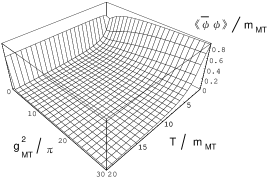
Figure 10: Fermion condensate in the MT model.

The numerical plot of the fermion condensate (5.6) is shown in Fig. 10. The condensate becomes smaller as $T$ grows at strong coupling. It should be noted again that the validity of the fermion condensate (5.6) is restricted within the DR regime. Thus, the condensate grows as $T$ becomes large in the negative-coupling regime but we cannot believe this result since it is out of the DR regime. In particular, we list the result in three regions below.

1. $g_{\rm\scriptscriptstyle{MT}}^{2}\,\gg\,\pi,~{}~{}T\,\gg\,m_{\rm\scriptscriptstyle{MT}}g_{\rm\scriptscriptstyle{MT}}/2\pi$ : We obtain

   $$\langle\langle\bar{\psi}\psi\rangle\rangle\;\sim\;2m_{\rm\scriptscriptstyle{MT}}\left(\frac{m_{\rm\scriptscriptstyle{MT}}g_{\rm\scriptscriptstyle{MT}}}{2\pi T}\right)^{2}\,\ll\,2m_{\rm\scriptscriptstyle{MT}}.$$

   In the limit $T\rightarrow\infty$, The condensate vanishes asymptotically and the chiral symmetry breaking is restored.

2. $g^{2}_{\rm\scriptscriptstyle{MT}}\,\gg\,\pi,~{}~{}T\,\ll\,m_{\rm\scriptscriptstyle{MT}}g_{\rm\scriptscriptstyle{MT}}/2\pi$ : The fermion condensate is approximately

   $$\langle\langle\bar{\psi}\psi\rangle\rangle\;\sim\;m_{\rm\scriptscriptstyle{MT}}\left(\frac{2T}{m_{\rm\scriptscriptstyle{MT}}}\right)^{\pi/g_{\rm\scriptscriptstyle{MT}}^{2}}.$$

   If $T$ is low enough, the condensate is also small. Note that the above result is valid only in the restricted region, $T\,\gtrsim\,m_{\rm\scriptscriptstyle{MT}}$.

3. $0\,<\,g_{\rm\scriptscriptstyle{MT}}^{2}\,\ll\,1,~{}~{}T\,\gg\,m_{\rm\scriptscriptstyle{MT}}/2\pi$ : The condensate tends to the constant value

   $$\langle\langle\bar{\psi}\psi\rangle\rangle\;\sim\;\frac{2m_{\rm\scriptscriptstyle{MT}}}{\pi}.$$

Moreover, we can define the parameter $q_{0}$ denoting the mean inter-particle distance by the inverse of the charge density, $q_{0}=\frac{1}{f_{+}}$, regardless of whether those are positively or negatively charged. Thus it is expressed by

$$q_{0}(g_{\rm\scriptscriptstyle{MT}},T) = \frac{2T}{m_{\rm\scriptscriptstyle{MT}}\langle\langle\,\bar{\psi}\psi\,\rangle\rangle}$$ (5.7)

$$= T\left(\frac{m_{\rm\scriptscriptstyle{MT}}}{2T}\right)^{(1+g_{\rm\scriptscriptstyle{MT}}^{2}/\pi)^{-1}}\!\!\gamma_{0}^{\prime}\,\left(\hat{z}\right)^{-1}.$$

Chiral Operators in Massive Thirring Model

The chiral operators (fermion density) of the MT model

$$\sigma_{\pm}\;=\;\bar{\psi}\left(\frac{1\pm\gamma^{5}}{2}\right)\psi,$$ (5.8)

corresponds to the positive charged particle and negative one, respectively. In terms of the components $\psi_{1}$ and $\psi_{2}$, $\sigma_{\pm}$ are defined by $\sigma_{+}\,=\,\psi^{\dagger}_{2}\psi_{1}$ and $\sigma_{-}\,=\,\psi^{\dagger}_{1}\psi_{2}$. The $\sigma_{\pm}$ transforms under the chiral transformation $\psi\rightarrow{\rm e}^{ia\gamma^{5}}\psi$ as

$$\sigma_{\pm}\longrightarrow\exp(\pm 2ia)\sigma_{\pm}.$$ (5.9)

In other words, Eq. (5.9) implies that $\sigma_{\pm}$ has a well-defined $\pm$ chiral charge. Thus the chiral invariant combination $\sigma_{+}\sigma_{-}$ is neutral in terms of the chiral charge. This neutral pair corresponds to the “molecule” in the CG system.

5.2 Monopole Condensate in Compact QED

We can interpret fundamental fermions in the MT model as monopoles in compact QED and so treat explicitly the monopole dynamics from that of the MT model. Recall that charged particles consisting of the CG system are inherently related to monopoles in compact QED. The positively and negatively charged particles in the CG system correspond to the chiral operators $\sigma_{+}$ and $\sigma_{-}$, respectively. In the four-dimensional language, a monopole and an anti-monopole correspond to the chiral operator $\sigma_{+}$ and $\sigma_{-}$, respectively. It would be expected that we could define the monopole (anti-monopole) operator $M$ ($\bar{M}$) by the chiral operator $\sigma_{+}$ ($\sigma_{-}$). Roughly speaking, we can effectively treat the quantum theory of monopoles as the chiral operators in the two-dimensional MT model through the PS mechanism, and the quantum MT model in two dimensions describes the effective theory of monopoles in four-dimensional compact QED. Thus we can identify the monopole condensate in compact QED with the fermion condensate in the MT model as follows:

$$\langle\langle\,M\,\rangle\rangle\;\equiv\;\langle\langle\,\bar{\psi}\psi\,\rangle\rangle,$$ (5.10)

where $\langle\langle\,\bar{M}\,\rangle\rangle\,=\,\langle\langle\,M\,\rangle\rangle$ since the net monopole charge is zero. We can express the fermion condensate by parameters of compact QED as follows:

$$\langle\langle\,M\,\rangle\rangle = \frac{\Lambda}{\sqrt{2}}\left(\frac{\sqrt{2}T}{\Lambda}\right)^{2\pi^{2}/g^{2}}\kappa^{\pi^{2}(g^{2}-2\pi^{2})/g^{4}}\gamma_{0}^{\prime}(\hat{z}),$$ (5.11)

$$\hat{z} = \frac{g^{2}}{2\pi^{3}}\left(\frac{2T^{2}}{\Lambda^{2}}\right)^{(\pi^{2}-g^{2})/g^{2}}\kappa^{2\pi^{2}(g^{2}-\pi^{2})/g^{4}}.$$ (5.12)

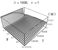
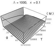
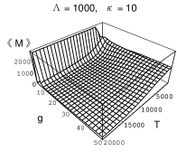
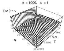
Fig. 11 (a) Fig. 11 (b) Fig. 11 (c) Fig. 11 (d)

Figure 11: Monopole Condensate.

The numerical plot of Eq. (5.11) is shown in Fig. 11. The behavior of the monopole condensate is almost same as the fermion condensate in the MT model. The condensate vanishes as $T\rightarrow\infty$ at strong coupling. In the weak-coupling regime, the condensate also becomes large as the temperature grows but this result is doubtful since it is out of the DR regime. In the same way as the MT model, we would not be able to believe the results at weak-coupling. Finally, we shall investigate analytically the condensate in the specific three regimes and list the results below.

1. $g^{2}\,\gg\,4\pi^{2},~{}~{}T\,\gg\,T^{\rm asy}_{{\rm cr}\,(l=1)}$ : The condensate is approximately

   $$\langle\langle\,M\,\rangle\rangle\;\sim\;\frac{\Lambda\,g^{2}}{\sqrt{2}\pi^{3}}\left(\frac{\Lambda}{T}\right)^{2}\,\kappa^{3\pi^{2}/g^{2}}\!\ll\,2\sqrt{2}\Lambda\,\kappa^{\pi^{2}/g^{2}}.$$

2. $g^{2}\,\gg\,4\pi^{2},~{}~{}T\,\ll\,T^{\rm asy}_{{\rm cr}\,(l=1)}$ : The condensate becomes

   $$\langle\langle\,M\,\rangle\rangle\;\sim\;\sqrt{2}\Lambda\,\kappa^{\pi^{2}/g^{2}}\left(\frac{\sqrt{2}T}{\kappa^{\pi^{2}/g^{2}}\Lambda}\right)^{\pi^{2}/g^{2}}.$$

3. $2\pi^{2}\,<\,g^{2}\,\ll\,2\pi^{2}+2\pi,~{}~{}T\,\gg\,(\Lambda/\sqrt{2}\pi)\,\kappa^{\pi^{2}/g^{2}}$ : Now, we obtain the condensate

   $$\langle\langle\,M\,\rangle\rangle\;\sim\;\frac{2\sqrt{2}\Lambda}{\pi}\,\kappa^{\pi^{2}/g^{2}}.$$

	MT at high temperature	One-dimensional CG	compact QED
Thermal Pressure	Fermions	Vortices	Monopoles
Large	Chirally Broken	Plasma	Confinement
Small	Chirally Symmetric	Molecule	Coulomb
Condensate	Fermion Condensate	Particle Density	Monopole Condensate
Non-zero	Chirally Broken	Plasma	Confinement
Zero	Chirally Symmetric	Molecule	Coulomb
Operators	$\sigma_{+},\;\sigma_{-}$, (chiral operators)	Vortex, Anti-vortex	Monopole, Anti-monopole
1-point Function	$\langle\langle\,\bar{\psi}\psi\,\rangle\rangle$ $\left(\,\langle\langle\,\sigma_{+}\,\rangle\rangle\,\right)$	$f_{+}\;(\,=\,f_{-}\,)$	$\langle\langle\,M\,\rangle\rangle\;(\,=\,\langle\langle\,\bar{M}\,\rangle\rangle\,)$
2-point Function	$\langle\langle\,\sigma_{+}\sigma_{-}\,\rangle\rangle$, $\langle\langle\,\sigma_{+}\sigma_{+}\,\rangle\rangle$	$f_{+-},\;f_{++}$	$\langle\langle\,M\bar{M}\,\rangle\rangle$, $\langle\langle\,MM\,\rangle\rangle$

Table 4: Relations of observables and phases in the MT model at high temperature, one-dimensional CG system and compact QED.

The mean inter-monopole distance can be rewritten by

$$q_{0}(g_{\rm\scriptscriptstyle{MT}},T) = \frac{1}{\langle\langle\,M\bar{M}\,\rangle\rangle}\sqrt{\frac{2}{\zeta}}\frac{T}{\Lambda}$$ (5.13)

$$= T\left(\sqrt{\frac{\zeta}{2}}\frac{\Lambda}{T}\right)^{2\pi^{2}/g^{2}}\gamma_{0}^{\prime}\,\left(\hat{z}\right)^{-1}.$$

5.3 Two-charge Correlators

The two-charge density functions in the CG system is given in Ref. [27] by

$$f_{+-}(X,\,Y) = \frac{1}{Z_{\rm 1CG}}\sum_{N=1}^{\infty}\frac{z^{2N}}{(N!)^{2}}\left(\prod_{i=1}^{2N}\int^{L}_{0}\!\!dx_{i}\right)\sum_{i=1}^{N}\sum_{j=N+1}^{2N}\delta(x_{i}-X)\delta(x_{j}-Y)$$ (5.14)

$$\times\exp\left[\frac{2\pi\sigma^{2}}{\theta}\!\!\!\!\sum_{1\leq i<j\leq 2N}\!\!\!\epsilon_{i}\epsilon_{j}|x_{i}-x_{j}|\right]$$

$$= \frac{1}{Z_{\rm 1CG}}\sum_{N=1}^{\infty}\frac{z^{2N}}{((N-1)!)^{2}}\left(\prod_{i=1}^{2N}\int^{L}_{0}\!\!dx_{i}\right)\delta(x_{N}-X)\delta(x_{2N}-Y)$$

$$\times\exp\left[\frac{2\pi\sigma^{2}}{\theta}\!\!\!\!\sum_{1\leq i<j\leq 2N}\!\!\!\epsilon_{i}\epsilon_{j}|x_{i}-x_{j}|\right],$$

$$f_{++}(X,\,Y) = \frac{1}{Z_{\rm 1CG}}\sum_{N=1}^{\infty}\frac{z^{2N}}{(N!)^{2}}\left(\prod_{i=1}^{2N}\int^{L}_{0}\!\!dx_{i}\right)\sum_{i=1}^{N}\sum_{i\neq j=1}^{N}\delta(x_{i}-X)\delta(x_{j}-Y)$$ (5.15)

$$\times\exp\left[\frac{2\pi\sigma^{2}}{\theta}\!\!\!\!\sum_{1\leq i<j\leq 2N}\!\!\!\epsilon_{i}\epsilon_{j}|x_{i}-x_{j}|\right]$$

$$= \frac{1}{Z_{\rm 1CG}}\sum_{N=1}^{\infty}\frac{z^{2N}}{N!(N-2)!}\left(\prod_{i=1}^{2N}\int^{L}_{0}\!\!dx_{i}\right)\delta(x_{N-1})\delta(x_{N}-Y)$$

$$\times\exp\left[\frac{2\pi\sigma^{2}}{\theta}\!\!\!\!\sum_{1\leq i<j\leq 2N}\!\!\!\epsilon_{i}\epsilon_{j}|x_{i}-x_{j}|\right].$$

By the use of Eq. (5.14) and (5.15), we can write the correlators of the chiral operators in the MT model at finite temperature, $\langle\langle\,\sigma_{+}(X)\sigma_{-}(0)\,\rangle\rangle$ and $\langle\langle\,\sigma_{+}(X)\sigma_{+}(0)\,\rangle\rangle$ as

$$\langle\langle\,T_{C}\sigma_{+}(X)\sigma_{-}(0)\,\rangle\rangle$$

$$= \left(\frac{T}{m_{\rm\scriptscriptstyle{MT}}}\right)^{2}\frac{1}{\left[4Q^{2}(X_{1},X_{2})\right]^{(1+g^{2}_{\rm\scriptscriptstyle{MT}}/\pi)^{-1}}}\exp\left[\frac{2\pi}{\beta}X_{1}\left(1+\frac{g^{2}_{\rm\scriptscriptstyle{MT}}}{\pi}\right)^{-1}\right]\,f_{+-}\left(z,\,\theta,\,\sigma\,;X_{1}\right),$$

$$\langle\langle\,T_{C}\sigma_{+}(X)\sigma_{+}(0)\,\rangle\rangle$$

$$= \left(\frac{T}{m_{\rm\scriptscriptstyle{MT}}}\right)^{2}\left[4Q^{2}(X_{1},X_{2})\right]^{(1+g^{2}_{\rm\scriptscriptstyle{MT}}/\pi)^{-1}}\exp\left[-\frac{2\pi}{\beta}X_{1}\left(1+\frac{g^{2}_{\rm\scriptscriptstyle{MT}}}{\pi}\right)^{-1}\right]\,f_{++}(z,\,\theta,\,\sigma\,;X_{1}),$$

where $z,\theta$ and $\sigma$ are defined by

$$z=\frac{m^{2}_{\rm\scriptscriptstyle{MT}}}{2T}\left(\frac{2T}{m_{\rm\scriptscriptstyle{MT}}}\right)^{(1+g^{2}_{\rm\scriptscriptstyle{MT}}/\pi)^{-1}},\quad\theta=T,\quad\sigma=T\sqrt{\frac{\pi}{\pi+g^{2}_{\rm\scriptscriptstyle{MT}}}}.$$ (5.18)

Here $X=(X_{1},X_{2})$ is the coordinate on the two-dimensional Euclidean space, and $T_{C}$ denotes the contour-ordering along $C=[0,-i\beta]$ and $Q^{2}(X_{1},X_{2})$ is defined by

$$Q^{2}(X_{1},X_{2})\;=\;\mathrm{sinh}\left(\frac{\pi}{\beta}(X_{1}+iX_{2})\right)\mathrm{sinh}\left(\frac{\pi}{\beta}(X_{1}-iX_{2})\right).$$ (5.19)

Using these functions, we can define the scale-independent ratio

$$R(g_{\rm\scriptscriptstyle{MT}},T;X)\;=\;\frac{1}{\left[4Q^{2}(X_{1},X_{2})\right]^{2(1+g^{2}_{\rm\scriptscriptstyle{MT}}/\pi)^{-1}}}\exp\left[\frac{4\pi}{\beta}X_{1}\left(1+\frac{g^{2}_{\rm\scriptscriptstyle{MT}}}{\pi}\right)^{-1}\right]\,\frac{f_{+-}(z,\theta,\sigma,;X)}{f_{--}(z,\theta,\sigma;X)}$$ (5.20)

Using the above quantities, we can also evaluate the condensate of a pair of the monopole and anti-monopole from the two-point function of the chiral operators $\sigma_{+}$ and $\sigma_{-}$ by identifying $\langle\langle\,\sigma_{+}\sigma_{-}\,\rangle\rangle\,(\,\langle\langle\,\sigma_{+}\sigma_{+}\,\rangle\rangle\,)$ with $\langle\langle\,M\bar{M}\,\rangle\rangle\,(\,\langle\langle\,MM\,\rangle\rangle\,)$. From the results of the previous subsection we can read off the expression of $\langle\langle\,M\bar{M}\,\rangle\rangle\,(\,\langle\langle\,MM\,\rangle\rangle\,)$ plugged with Eq. (3.34) as

$$\langle\langle\,M\bar{M}\,\rangle\rangle\quad(\;=\;\langle\langle\,\bar{M}M\,\rangle\rangle\;)$$

$$= \frac{T^{2}}{2\zeta\Lambda^{2}}\frac{1}{\left[4Q^{2}(X_{1},X_{2})\right]^{2\pi^{2}/g^{2}}}\exp\left[\frac{4\pi^{3}}{g^{2}}\frac{X_{1}}{\beta}\right]\,f_{+-}\left(z,\,\theta,\,\sigma\,;X_{1}\right),$$

$$\langle\langle\,MM\,\rangle\rangle\quad(\;=\;\langle\langle\,\bar{M}\bar{M}\,\rangle\rangle\;)$$

$$= \frac{T^{2}}{2\zeta^{2}\Lambda^{2}}\left[4Q^{2}(X_{1},X_{2})\right]^{2\pi^{2}/g^{2}}\exp\left[-\frac{4\pi^{3}}{g^{2}}\frac{X_{1}}{\beta}\right]\,f_{++}(z,\,\theta,\,\sigma\,;X_{1}),$$

where $z,\theta$ and $\sigma$ are defined by

$$z=\frac{\zeta\Lambda^{2}}{T}\left(\sqrt{\frac{2}{\zeta}}\frac{T}{\Lambda}\right),\quad\theta=T,\quad\sigma=\frac{\sqrt{2}\pi}{g}T.$$ (5.23)

The scale-independent ratio is given by

$$R(g,\zeta,T;X)\;=\;\frac{1}{\left[4Q^{2}(X_{1},X_{2})\right]^{4\pi^{2}/g^{2}}}\exp\left[\frac{8\pi^{3}}{g^{2}}\frac{X_{1}}{\beta}\right]\,\frac{f_{+-}(z,\theta,\sigma,;X)}{f_{--}(z,\theta,\sigma;X)}.$$ (5.24)

The neutral pair condensate $\langle\langle\,M\bar{M}\,\rangle\rangle$ is much larger than $\langle\langle\,MM\,\rangle\rangle$ one at short distance (but yet large distance compared to ($2\pi T)^{-1}$) as discussed in detail in Ref. [21]. That is, the system tends to form the $M\bar{M}$ pairs (“monopole bound states”) at high temperature. Of course, the behavior of those agrees with the physical expectation as noted in Introduction. For large distance, no bound states are formed ($R$ tends to 1). The $R$ is almost 1 at the certain value $X_{1}$.

6 Conclusions and Discussions

We have investigated a phase structure of compact QED by considering the system as a perturbative deformation from the topological model. Phases of compact QED are determined by the behavior of the CG system in an $O(2)$NLSM₂. In this paper, in order to discuss the behavior of the CG system, we have utilized a one-dimensional CG approximation and the thermal pressure that can be exactly calculated [27]. The thermal pressure of the one-dimensional CG system can be also expressed by parameters of compact QED. From the result we could study a phase structure of compact QED with strong coupling and at high temperature. The critical-line equation has been explicitly evaluated. In particular, the asymptotic form of the critical-line equation derived in this paper is precisely identical with the result given by a perturbative method (one-loop potential calculation) in our previous work [15]. A one-dimensional CG approximation does not on a perturbation theory in two-dimensions, and hence this result is non-trivial and further confirmation for the expression of the critical-line equations in the sufficiently high-temperature and strong-coupling regime of compact QED. We have also discussed the relation between the chiral symmetry restoration in the two-dimensional MT model and monopole condensate in the four-dimensional compact QED by using some exact results in the one-dimensional CG system. In particular, we have evaluated the monopole condensate in our scenario and discussed the quantum theory of monopoles from the viewpoint of the MT model. We might be able to relate the SG/MT duality in two dimensions to the electric/magnetic duality in four dimensions through the PS dimensional reduction. The two-dimensional MT model, SG model and CG system are not only interesting as the model in the statistical mechanics but also very useful to develop the techniques which may be applicable to more realistic four-dimensional QCD as also noted in Ref. [21]. In particular, the MT model may be considered to be the toy model of QCD. It should be remarked that at low temperature where the quarks and gluons are strongly confined into hadrons, one can describe the system by an effective chiral bosonic Lagrangian (CBL) for the lightest mesons (pions, kaons and eta) which are the Nambu Goldstone bosons of the chiral symmetry breaking. The relationship between the original fermionic QCD and the chiral bosonic theory has many similarities with the duality between the SG and MT model. Moreover, it would possibly be related to the above analogy, compact QED is also interesting in the context of QCD with the maximal Abelian gauge fixing. Once this gauge fixing is chosen, the full QCD is thought to be described by compact $U(1)$ gauge theory in the low energy (infrared) regime i.e., strongly-coupled regime. This phenomenon is called “Abelian dominance,” confirmed by numerical simulations in the lattice gauge theory. Thus compact QED is one of the most interesting subjects in the particle physics and well-suited to develop the techniques for studying the confinement in non-abelian gauge theories, such as QCD. Finally, we comment on the future problems. In our previous works [14, 15], we have obtained some plausible and consistent results but our considerations are restricted within the high-temperature and strong-coupling regime. For a example, the low-temperature regime near critical coupling is too difficult to study. However, we expect that the low-temperature regime near the critical coupling can be approached by the use of the Gaussian effective potential (GEP) that can describe a confining phase transition at zero temperature. We could study more intensively in this approach the critical behavior of compact QED at low temperature [17]. Furthermore, we think that the recent results of Ref. [28] would be useful to study the weak-coupling region of compact QED, $g<\pi$. This would be very interesting approach.

Acknowledgements

The author thanks W. Souma, M. Ishibashi and M. Hamanaka for their encouragement, useful discussions and valuable comments. He also would like to acknowledge H. Aoyama and K. Sugiyama.

Appendix A Critical Coupling from BKT Phase Transition

Let us consider a pair of vortices at a finite distance $r_{12}$ in a box with size $L$. From Eq. (3.5) the global contribution of a vortex pair to the partition function is, for dimensional reasons, of the form

$$Z_{\rm pair} \sim \int_{r_{12}>R_{0}}d^{2}x_{1}d^{2}y_{1}\,\exp\left(-\frac{4\pi^{2}}{g^{2}}\,\ln\frac{r_{12}}{R_{0}}\right)$$ (A.1)

$$\sim L^{4}\exp\left(-\frac{4\pi^{2}}{g^{2}}\,\ln\frac{L}{R_{0}}\right).$$

Therefore we obtain the contribution to the free energy,

$$F_{\rm pair}\;\sim\;\ln Z_{\rm pair}\;\sim\;\left(4-\frac{4\pi^{2}}{g^{2}}\right)\,\ln L.$$ (A.2)

If $g<\pi$, this is negligible in the limit $L\rightarrow\infty$. While, if $g>\pi$, the system becomes unstable. The well-separated vortices tend to be created and the disorder increases. Thus we can estimate the critical-coupling as $g_{\rm cr}=\pi$. It corresponds to the critical temperature of the CG system $T_{\rm CG}=1/8\pi$, at which the BKT phase transition occurs.

Appendix B Finite-Size Effect of Cylinder

A massless free boson field theory is a conformal field theory with the central charge $c=1$. Using the mapping from the infinite plane (with holomorphic coordinate $z$) to the cylinder of circumference $\beta\equiv 1/T$ (with coordinate $w$),

$$w\;=\;\frac{\beta}{2\pi}\,\ln z~{}~{}(z={\rm e}^{2\pi w/\beta}),$$ (B.1)

we can obtain the free boson theory on the cylinder, and the free energy per unit length is shifted by

$$\Delta f\;=\;-\frac{\pi}{6}T^{2},$$ (B.2)

due to the finite-size effect of the cylinder. Thus the free energy is shifted by

$$F\;=\;-\frac{\pi}{6}T^{2}L,$$ (B.3)

and the partition function is given by

$$Z\;=\;{\rm e}^{-\beta F}\;=\;\exp\left(\frac{\pi}{6}LT\right).$$ (B.4)

As a result, the additional pressure

$$P(T)\;=\;\frac{\pi}{6}T^{2},$$ (B.5)

arises from the geometry of the cylinder.

Appendix C One-Loop Effective Potential of the Sine-Gordon Model

The one-loop effective potential of the two-dimensional SG model at finite temperature [29] is given by

$$V_{1{\rm loop}}(\phi_{c}) = V_{\rm 0}(\phi_{c})+V_{\rm FT}(\phi_{c}),$$ (C.1)

$$V_{\rm 0}(\phi_{c}) \equiv \frac{m^{2}}{8\pi}\cos\left(\frac{\sqrt{\lambda}}{m}\phi_{c}\right)\left[1-\ln\cos\left(\frac{\sqrt{\lambda}}{m}\phi_{c}\right)\right],$$ (C.2)

$$V_{\rm FT}(\phi_{c}) \equiv \frac{1}{\pi\beta^{2}}\int^{\infty}_{0}dx\ln\left[1-\exp\left(-\sqrt{x^{2}+M^{2}(\phi_{c})\beta^{2}}\right)\right],$$ (C.3)

$$M^{2}(\phi_{c}) \equiv m^{2}\cos\left(\frac{\sqrt{\lambda}}{m}\phi_{c}\right).$$ (C.4)

The second equation (C.2) is the temperature-independent part and corresponds to the zero temperature result. The third equation (C.3) is the temperature-dependent part and describes the thermal effect. It vanishes in the zero temperature limit, $\beta\rightarrow\infty$ . The minimum of the potential $\phi_{c}=0$ is still stable under one-loop quantum fluctuations at zero temperature. Taking the second derivative of Eq. (C.1) with respect to $\phi_{c}$ at $\phi_{c}=0$, one can evaluate the critical-line equation [30] as

$$m^{2}(\beta) = m^{2}+\left.\frac{\partial^{2}V_{\rm FT}}{\partial\phi_{c}^{~{}2}}\right|_{\phi_{c}=0}$$ (C.5)

$$= m^{2}-m^{2}\frac{\bar{\lambda}}{2\pi}f(\bar{\beta})=0,$$

where $\bar{\lambda}\equiv\lambda/m^{2}$, $\bar{\beta}\equiv\beta m$ and $f(\bar{\beta})$ is defined by

$$f(\bar{\beta})\equiv\int^{\infty}_{0}\!\!\!dx\,\frac{1}{\sqrt{\bar{\beta}^{2}+x^{2}}\left[\exp\left(\sqrt{\bar{\beta}^{2}+x^{2}}\right)-1\right]}.$$ (C.6)

Thus the critical-line equation is given by

$$1-\frac{\bar{\lambda}}{2\pi}f(\bar{\beta})=0.$$ (C.7)

Parameters of the SG model can be expressed by those of compact QED and hence we obtain

$$\bar{\beta}\;=\;\frac{4\pi^{3/2}}{gT}\,\zeta^{1/2}\Lambda,\qquad\bar{\lambda}=\frac{8\pi^{3}}{g^{2}},$$ (C.8)

where one should remember that $\zeta$ is defined by

$$\zeta\equiv\kappa^{2\pi^{2}/g^{2}},\qquad\kappa\equiv\frac{R_{0}}{a}.$$ (C.9)

Therefore the critical-line equation can be rewritten as

$$1-\frac{4\pi^{2}}{g^{2}}f\left(\frac{4\pi^{3/2}\zeta^{1/2}}{gT}\right)=0.$$ (C.10)

The numerical plots of Eq. (C.10) are shown in Fig. 12.

Figure 12: The phase structure of a compact $U(1)$ gauge theory estimated by the one-loop effective potential of the SG model.

The above (below) of the plotted-lines corresponds to a Coulomb (confining) phase. It should be noted that the validity of this derivation is restricted within the strong-coupling regime of compact QED. In the weak-coupling and high-temperature regime of the SG model, the critical-line Eq. (C.7) is reduced to the simple form,

$$T_{\rm cr}\;=\;\frac{4m^{3}}{\lambda},$$ (C.11)

which denotes the critical-temperature of the SG model. Combining Eq. (3.26) with Eq. (C.11) leads to

$$T_{\rm cr}\;=\;\frac{2\zeta^{1/2}\Lambda}{\pi^{3/2}}\,g\;=\;\frac{2\Lambda\kappa^{\pi^{2}/g^{2}}}{\pi^{3/2}}\,g,$$ (C.12)

which is the critical-temperature of compact QED with strong coupling and at high temperature. The SG model with weak coupling corresponds to compact QED with strong one, and hence we can reliably evaluate the strong-coupling regime of compact QED since one-loop effective potential calculations are valid in the weakly coupled SG model. This fact is one of the greatest advantages in our scenario.

References

- [1] K. Wilson, “Confinement of quarks,” Phys. Rev. D 10 (1974) 2445.
-
[2]
A.M. Polyakov, “Compact gauge theories and the infrared
catastrophe,” Phys. Lett. B 59 (1975)
82.
A.M. Polyakov, “Quark confinement and topology of gauge theories,” Nucl. Phys. B 120 (1977) 429. - [3] T. Banks, R. Myerson and J. Kogut, “Phase transitions in abelian lattice gauge theories,” Nucl. Phys. B 129 (1977) 493.
- [4] R. Savit, “Topological excitations in U(1) invariant theories,” Phys. Rev. Lett. 39 (1977) 55.
- [5] S.D. Drell, H.R. Quinn, B. Svetitsky and M. Weinstein, “QED on a lattice: A Hamiltonian variational approach to the physics of the weak coupling region,” Phys. Rev. D 19 (1979) 619.
- [6] K. Osterwalder and E. Seiler, “Gauge field theories on the lattice,” Ann. Phys. 110 (1978) 440.
- [7] A. Guth, “Existence proof of a nonconfining phase in four-dimensional U(1) lattice gauge theory,” Phys. Rev. D 21 (1980) 2291.
- [8] M.E. Peskin, “Mandelstam-’t Hooft duality in abelian lattice models,” Ann. Phys. 113 (1978) 122.
-
[9]
Y. Nambu, “Strings, monopoles and gauge fields,”
Phys. Rev. D 10 (1974) 4262.
G. ’t Hooft, in: High Energy Physics, edited by A. Zichichi (Editorice Compositori, Bologna, 1975).
S. Mandelstam, “Vortices and quark confinement in nonabelian gauge theories,” Phys. Rep. 23 (1976) 245. -
[10]
K.-I. Kondo, “Yang-Mills theory as a deformation of
topological field theory, dimensional reduction and quark
confinement,” Phys. Rev. D 58 (1998) 105019,
hep-th/9801024.
K.-I. Kondo, “A formulation of the Yang-Mills theory as a deformation of a topological field theory based on background field method,” Int. J. Mod. Phys. A 16 (2001) 1303, hep-th/9904045. -
[11]
H. Hata and Y. Taniguchi, “Finite temperature
deconfining transition in the BRST formalism,”
Prog. Theor. Phys. 93 (1995) 797, hep-th/9405145.
H. Hata and Y. Taniguchi, “Color confinement in perturbation theory from a topological model,” Prog. Theor. Phys. 94 (1995) 435, hep-th/9502083. - [12] K.-I. Izawa, “Another perturbative expansion in nonabelian gauge theory,” Prog. Theor. Phys. 90 (1993) 911, hep-th/9309150.
- [13] K. Yoshida, “The effect of the boundary conditions in the reformulation of ,” JHEP 07 (2000) 007, hep-th/0004184.
- [14] K. Yoshida, “Deconfining phase transition in QCD4 and QED4 at finite temperature,” JHEP 04 (2001) 030, hep-th/0012237.
- [15] K. Yoshida and W. Souma, “Phase structure of a compact gauge theory from the viewpoint of a sine-Gordon model,” Phys. Rev. D 64 (2001) 125002, hep-th/0103075.
- [16] K. Yoshida, “Confining phases of a compact gauge theory from the sine-Gordon/massive Thirring duality,” hep-th/0110153.
- [17] K. Yoshida and W. Souma, “Phase structure of compact QED - Gaussian effective potential approach,” in preparation.
- [18] G. Parisi and N. Sourlas, “Random magnetic fields, supersymmetry, and negative dimensions,” Phys. Rev. Lett. 43 (1979) 744.
- [19] K.-I. Kondo, “Existence of confinement phase in quantum electrodynamics,” Phys. Rev. D 58 (1998) 085013, hep-th/9803133.
-
[20]
V.L. Berezinskii, “Destruction of long-range order
in one-dimensional and two-dimensional systems having a
continuous symmetry group I. classical systems,”
Sov. Phys. JETP. 32 (1971) 493.
J.M. Kosterlitz and D.V. Thouless, “Ordering, metastability and phase transition in two-dimensional systems,” J. Phys. C 6 (1973) 1181.
J.M. Kosterlitz, “The critical properties of the two dimensional XY model,” J. Phys. C 7 (1974) 1046. - [21] A.Gomez Nicola, R.J. Rivers and D.A. Steer, “Chiral symmetry restoration in the massive Thirring model at finite T and : Dimensional reduction and the Coulomb gas,” Nucl. Phys. B 570 (2000) 475, hep-th/9906236.
-
[22]
N. Parga, “Finite temperature behavior of topological
excitations in lattice compact QED,”
Phys. Lett. B 107 (1981) 442.
B. Svetitsky and L.G. Yaffe, “Critical behavior at finite-temperature confinement transitions,” Nucl. Phys. B 210 (1982) 423.
B. Svetitsky, “Symmetry aspects of finite-temperature confinement transitions,” Phys. Rep. 132 (1986) 1. - [23] J. Zinn-Justin, “Quantum Field Theory and Critical Phenomena,” Clarendon Press, Oxford, 1993.
- [24] S. Coleman, “Quantum sine-Gordon equation as the massive Thirring model,” Phys. Rev. D 11 (1975) 2088.
- [25] D. Delpine, R. Gonzlez Felipe and J. Weyers, “Equivalence of the sine-Gordon and massive Thirring models at finite temperature,” Phys. Lett. B 419 (1998) 296, hep-th/9709039.
- [26] A.Gmez Nicola and D.A. Steer, “Thermal bosonization in the sine-Gordon and massive Thirring models,” Nucl. Phys. B 549 (1999) 409, hep-ph/9810519.
-
[27]
A. Lenard, “Exact statistical mechanics of a
one-dimensional system with Coulomb
forces,” J. Math. Phys. 2 (1961) 682.
S.F. Edwards and A. Lenard, “Exact statistical mechanics of a one-dimensional system with Coulomb forces. II. The method of functional integration,” J. Math. Phys. 3 (1962) 778. - [28] M. Faber and A.N. Ivanov, “On the equivalence between sine-Gordon model and Thirring model in the chirally broken phase of the Thirring model,” hep-th/0105057.
-
[29]
K.B. Joseph and V.C. Kuriakose, “Effective
potential in sine-Gordon theory at finite temperature,”
Phys. Lett. A 88 (1982) 447.
W.H. Kye, S.I. Hong and J.K. Kim, “Phase transition of the sine-Gordon theory at finite temperature,” Phys. Rev. D 45 (1992) 3006.
D.K. Kim, S.I. Hong, M.H. Lee and I.G. Koh, “Phase structure of the sine-Gordon model at finite temperature and volume,” Phys. Lett. A 191 (1994) 379. -
[30]
C.W. Bernard, “Feynman rules for gauge theories
at finite temperature,” Phys. Rev. D 9 (1974) 3312.
L. Dolan and R. Jackiw, “Symmetry behavior at finite temperature,” Phys. Rev. D 9 (1974) 3320.
H.E. Haber and H.A. Weldon, “Finite temperature symmetry breaking as Bose-Einstein condensation,” Phys. Rev. D 25 (1982) 502.