Cosmological Models and Renormalization Group Flow

Abstract:

We study cosmological solutions of Einstein gravity with a positive cosmological constant in diverse dimensions. These include big-bang models that re-collapse, big-bang models that approach de Sitter acceleration at late times, and bounce models that are both past and future asymptotically de Sitter. The re-collapsing and the bounce geometries are all tall in the sense that entire spatial slices become visible to a comoving observer before the end of conformal time, while the accelerating big-bang geometries can be either short or tall. We consider the interpretation of these cosmological solutions as renormalization group flows in a dual field theory and give a geometric interpretation of the associated c-function as the area of the apparent cosmological horizon in Planck units. The covariant entropy bound requires quantum effects to modify the early causal structure of some of our classical big-bang solutions.

1 Introduction

There has been considerable recent interest in the study of gravity with a positive cosmological constant $\Lambda$. This is in part due to cosmological observations indicating that our universe is undergoing accelerated expansion compatible with a small positive $\Lambda$ [1], but also because of various interesting theoretical issues that arise, see e.g. [2] - [9]. In particular, it has been conjectured that gravity in $n{+}1$-dimensional de Sitter spacetime has a dual description as a Euclidean conformal field theory in $n$ dimensions [9]. The proposed dS/cft duality has been extended to more general spacetime geometries that are asymptotically de Sitter, with cosmological evolution interpreted as a renormalization group flow on the field theory side [10, 11]. The physics is in some respects analogous to that of the much better understood adS/cft duality and related renormalization group flows [12], but other aspects are clearly quite different. For one thing, supersymmetry is absent from de Sitter gravity. Another important feature is the finite area of the de Sitter event horizon [13], which has been argued to put a finite upper limit on the number of available degrees of freedom in de Sitter gravity [4, 5, 14]. This would in turn imply that the proposed dS/cft duality could only be exact in the limit of infinite de Sitter entropy, that is vanishing $\Lambda$ [15].

In the present paper we study dS/cft related issues in a relatively simple context. In section 2 we present a number of analytic cosmological solutions of gravity with positive $\Lambda$ in various spacetime dimensions. We restrict our attention to homogeneous and isotropic cosmological models with perfect fluid matter and linear equations of state. This rather restricted framework yields a surprisingly rich set of exact solutions, which include big-bang models that approach de Sitter acceleration in the asymptotic future, re-collapsing big-bang models, and bounce geometries that approach de Sitter behavior both in the asymptotic past and asymptotic future. In section 3 we analyze the causal structure of the various solutions. This is followed, in section 4, by a discussion of cosmological horizons, both event horizons and apparent horizons. In section 5 we consider the interpretation of cosmological evolution as a renormalization group flow in a dual field theory. In particular, we identify the associated c-funtion with the area of the apparent cosmological horizon in Planck units. The c-theorem then becomes a geometric statement about the increase of the apparent horizon area in an expanding asymptotically de Sitter spacetime. We close with the observation that the covariant entropy bound [16] is violated at very early times in some of these models. The violation may, however, be traced to a region of spacetime where quantum gravity effects are expected to be important.

During the course of this work, there has been considerable activity in this area of research and papers have appeared on related topics. We note in particular [17], which studies cosmological models in Einstein gravity coupled to a scalar field with emphasis on their interpretation as renormalization group flows, and [18], which considers perfect fluid models and contains some of the solutions that we present below.

2 Cosmological models with positive vacuum energy

We consider $n{+}1$-dimensional homogeneous and isotropic cosmological models with $n\geq 2$ and a positive cosmological constant. The analysis of such models in 3+1 dimensions is standard material, see for example [19, 20], and many qualitative features carry over to general dimensions. The metric can be put into Robertson-Walker form,

$$ds^{2}=-dt^{2}+R^{2}(t)\left({dr^{2}\over 1-kr^{2}}+r^{2}d\Omega_{n-1}^{2}\right)\,,$$ (1)

where $d\Omega_{n-1}^{2}$ is the line element of an $n{-}1$-dimensional unit sphere. The geometry of constant $t$ slices depends on the sign of the parameter $k$, being spherical for $k>0$, flat for $k=0$, and hyperbolic for $k<0$. It is common to rescale the spatial coordinates in such a way as to make $k$ equal to $1,0,$ or $-1$, but we will not do that here. Instead we choose to retain the freedom to rescale the coordinates and our results will be given in terms of parameters that are invariant under such rescalings.

We take the matter to be a perfect fluid. Einstein’s equation and energy-momentum conservation can then be expressed as

$$\left({dR\over dt}\right)^{2} = {2\over n(n-1)}\left[\Lambda+8\pi G\rho\right]R^{2}-k\,,$$ (2)

$${d\rho\over dR} = -{n\over R}(\rho+P)\,.$$ (3)

We will restrict our attention to equations of state of the form

$$P=\alpha\rho\,,$$ (4)

with constant $\alpha$. Two cases of interest are radiation (with $\alpha=1/n$) and dust (with $\alpha=0$).

Equation (3) integrates to

$$\log{\rho}=-(1+\alpha)n\,\log{R}+const\,.$$ (5)

The integration constant can be expressed in terms of the scale factor at ‘cross-over’, i.e. when the matter energy density equals the vacuum energy density,

$$R=R_{*}\longleftrightarrow\rho=\rho_{\Lambda}={\Lambda\over 8\pi G}\,,$$ (6)

or equivalently

$${\rho\over\rho_{\Lambda}}=\left({R_{*}\over R}\right)^{(1+\alpha)n}\,.$$ (7)

Inserting this into equation (2) gives

$$\left({dR\over dt}\right)^{2}={2\Lambda\over n(n-1)}\left[1+\left({R_{*}\over R}\right)^{(1+\alpha)n}\right]R^{2}-k\,.$$ (8)

Now introduce a dimensionless time variable $\tau=\sqrt{2\Lambda\over n(n-1)}\,t$ and define $u=R/R_{*}$ to obtain

$$\left({du\over d\tau}\right)^{2}=u^{2}+u^{-(1+\alpha)n+2}-\kappa\,,$$ (9)

where $\kappa={n(n-1)\,k\over 2\Lambda R_{*}^{2}}$ is a dimensionless quantity. We observe that, while both $k$ and $R_{*}$ change under rescaling of the spatial coordinates, $\kappa$ is invariant. We also note that equation (9) only involves the combination $(1+\alpha)n$, which means in particular that the evolution for pressureless dust in $n{+}1$ dimensions is identical to that for radiation in one less dimension.

Figure 1: A typical potential for the equivalent particle motion.

Various values of $n$ and $\alpha$ yield simple analytic solutions and we analyze some of these below. We can, however, get a qualitative picture of the solutions for any $n$ and $\alpha$ by rewriting equation (9) as

$$\left({du\over d\tau}\right)^{2}+v(u)=-\kappa\,,$$ (10)

and proceeding by analogy with one-dimensional particle motion in the potential

$$v(u)=-u^{2}-u^{-(1+\alpha)n+2}\,.$$ (11)

The corresponding analysis for 3+1-dimensional cosmological models is carried out in [19]. A typical potential is drawn in figure 1. The parameter $-\kappa$ plays the role of the total energy of the particle. For $\kappa$ below a certain value $\kappa_{0}$, or equivalently, a total energy above the maximum of the potential, the particle can roam from $u=0$ to $u\rightarrow\infty$ and one obtains big-bang solutions that eventually approach de Sitter acceleration. Time-reversed solutions, describing a past asymptotically de Sitter universe that ends in a big crunch singularity, are also allowed.

Geometries with $\kappa>\kappa_{0}$, on the other hand, correspond to a total energy below the maximum of $v(u)$. The particle is then either confined to small values of $u$, resulting in big-bang solutions that re-collapse to a big crunch, or the particle comes in from large $u$ and is reflected off the potential barrier. These reflecting ‘bounce’ solutions are less realistic than the big-bang geometries from the point of view of cosmology but, being both past and future asymptotically de Sitter, they may prove useful for exploring the dS/cft correspondence. Finally, we have the Einstein static universe with $\kappa=\kappa_{0}$, corresponding to the particle perched in unstable equilibrium at the top of the potential.

2.1 Spatially flat models

It is always useful to have explicit solutions to work with and in the following we present several examples. We begin by restricting our attention to spatially flat models with $\kappa=0$. In this case, an exact solution to the evolution equation (9) for any combination of $n$ and $\alpha$ is given by [18]

$$u(\tau)=\sinh^{\beta}({\tau\over\beta})\,,$$ (12)

with $\beta={2\over(1+\alpha)n}$. These solutions describe big-bang geometries that expand from an initial singularity. They eventually enter an accelerating phase and are future asymptotically de Sitter. We have placed the origin of our time coordinate, $\tau=0$, at the initial singularity. For small $\tau$ the scale factor is

$$u(\tau)\approx\left({\tau\over\beta}\right)^{\beta}\,,$$ (13)

which is the expected behavior for the early universe. At late times the cosmological term takes over and we instead find

$$u(\tau)\approx 2^{-\beta}\,e^{\tau}\,,$$ (14)

which is de Sitter behavior.

These are by no means generic models, given that the matter energy density has been fine tuned to give $k=0$, but the special case $\beta=2/3$, which is found in [21] and corresponds to pressureless dust in 3+1 dimensions, appears to fit the observed universe rather well today [1]. In order to exhibit the full range of behavior outlined earlier, including re-collapsing universes and bounce geometries, one has to allow generic matter energy density, i.e. $\kappa\neq 0$. In this more general case, explicit solutions are only found for certain combinations of $n$ and $\alpha$ and we work out some of these below.

2.2 Radiation models in 3+1 dimensions

Let us consider $n=3$ and matter in the form of radiation with $\alpha={1/3}$. The same evolution is obtained for $n=4$ and $\alpha=0$, which corresponds to dust in $4+1$ dimensions. The equivalent one-dimensional potential reduces to $v(u)=-u^{2}-u^{-2}$, with a maximum at $u_{0}=1$ that corresponds to $\kappa_{0}=2$. It is then straightforward to integrate equation (9) and obtain the scale factor in closed form. The qualitative physical behavior of these solutions is well known [19] and depends on the value of $\kappa$ and the boundary conditions imposed on the integration.

2.2.1 Big-bang solutions

We begin with big-bang geometries that expand from an initial singularity. The solution takes the form

$$u(\tau)=\sqrt{\sinh{2\tau}+(\kappa/2)(1-\cosh{2\tau})}\,,$$ (15)

where we have used time-translation symmetry to put the initial singularity at $\tau=0$. This relatively simple expression for the scale factor is valid for any value of $\kappa$ and thus covers all three cases of positive, flat, and negative spatial curvature. All these models have the same initial rate of expansion,

$$u(\tau)\approx\sqrt{2\tau}\,,$$ (16)

as expected for a radiation-dominated universe in $3+1$ dimensions (or pressureless dust in $4{+}1$ dimensions) but the late time behavior is governed by the value of $\kappa$. For matter energy densities, such that $\kappa<2$, the vacuum energy density eventually dominates and the scale factor ultimately approaches the exponential expansion of de Sitter spacetime,

$$u(\tau)\approx{\sqrt{2-\kappa}\over 2}\,e^{\tau}\quad{\rm as}\quad\tau\rightarrow\infty\,.$$ (17)

Note that the dividing line between eternal expansion and re-collapse does not occur at the spatially flat solution. In the presence of a cosmological constant we can in fact have an ever expanding geometry with spherical spatial sections that are finite in extent at any given cosmic time. In such a universe the matter energy density is large enough to give closed spatial sections but not enough to overcome the effect of the positive cosmological constant.

If, on the other hand, the matter energy density is large enough to give $\kappa>2$ the universe expands to a maximum size,

$$u_{max}=\sqrt{{\kappa\over 2}-\sqrt{{\kappa^{2}\over 4}-1}}\,,$$ (18)

and then re-contracts back to zero scale factor at a finite time,

$$\tau_{f}={1\over 2}\,\log\left({\kappa+2\over\kappa-2}\right)\,.$$ (19)

As $\kappa\rightarrow 2^{+}$ the total lifetime, $\tau_{f}$, before the universe ends in a big-crunch, becomes arbitrarily long. As $\kappa\rightarrow\infty$, however, the matter energy dominates and the total lifetime is vanishing on the timescale set by $\Lambda$. One can then expand the hyperbolic functions in equation (15) to leading orders to recover the behavior of a re-collapsing $3{+}1$-dimensional universe with radiation and $\Lambda=0$,

$$u(\tau)\propto\sqrt{{\tau\over\tau_{f}}-{\tau^{2}\over\tau^{2}_{f}}}\,.$$ (20)

The ratio of matter and vacuum energy densities is given by

$${\rho\over\rho_{\Lambda}}={1\over u^{4}(\tau)}\,.$$ (21)

Since $u_{max}<1$ for all $\kappa>2$, the matter energy density exceeds the vacuum energy density at all times in the re-collapsing geometries.

Figure 2: The scale factor $u$ as a function of $\tau$ for big-bang models with matter in form of radiation and $\kappa=2.2$ (solid curve), $\kappa=2.0$ (dotted curve), and $\kappa=1.8$ (dashed curve).

Finally, there is the borderline case of $\kappa=2$ where the expansion slows down with time and the scale factor approaches a fixed value from below,

$$u(\tau) = \sqrt{1-e^{-2\tau}}$$ (22)

$$\rightarrow 1\quad{\rm as}\quad\tau\rightarrow\infty\,.$$

This solution, which approaches the Einstein static universe, is unstable in the sense that if $\kappa$ deviates at all from $2$ the universe eventually finds itself collapsing back to zero size or undergoing exponential expansion. Figure 2 depicts the scale factor for big-bang models with different values of $\kappa$.

2.2.2 Bounce solutions

These solutions only occur for $\kappa>2$ and therefore have spherical spatial sections. The spacetime geometry is non-singular and asymptotically de Sitter both in the past and future. Initially the scale factor is decreasing but after reaching a finite minimum value it bounces back and eventually approaches exponential de Sitter expansion. The ‘bounce’ solutions are given by

$$u(\tau)=\sqrt{{\kappa\over 2}+\sqrt{{\kappa^{2}\over 4}-1}\,\cosh 2\tau}\,,$$ (23)

where we have chosen the zero of the time coordinate to be when the scale factor takes its minimum value,

$$u_{min}=u(0)=\sqrt{{\kappa\over 2}+\sqrt{{\kappa^{2}\over 4}-1}}\,.$$ (24)

Note that $u_{min}>1$ for all $\kappa>2$ so, by equation (21), the vacuum energy exceeds the matter energy at all times. Examples of bounce geometries are displayed in figure 3.

Figure 3: The scale factor $u$ as a function of $\tau$ for bounce models in 3+1 dimensions. The dotted curve is for $\kappa=2.01$ and the solid curve is for $\kappa=3$.

In the limit $\kappa\rightarrow 2^{+}$ the solution spends a long time ‘near’ the Einstein static geometry. In the opposite limit, $\kappa\rightarrow\infty$, it instead approaches pure de Sitter space. To see this, consider the energy density at $\kappa\gg 1$, for which $u_{min}\approx\sqrt{\kappa}\gg 1$. It then follows from equation (21) that the matter energy density is vanishing compared to the vacuum energy at all times and the geometry must reduce to the de Sitter vacuum. The same conclusion can also be reached by explicit calculation, writing the Robertson-Walker line element (1) in terms of our dimensionless variables, inserting (23) for $u(\tau)$, and observing that the line element reduces in the $\kappa\rightarrow\infty$ limit to that of de Sitter spacetime in global coordinates.

All the $\kappa>2$ solutions are time-symmetric around some reference time, at which the scale factor is at an extremum. The $\kappa<2$ big-bang solutions are, on the other hand, asymmetric between the initial singularity and the future asymptotic de Sitter expansion, but time-reversed solutions, with de Sitter contraction in the asymptotic past and ending in a big crunch singularity, are also allowed.

2.3 Dust in 3+1 dimensions or radiation in 2+1 dimensions

Qualitative features of $3{+}1$-dimensional cosmological models, with $\Lambda>0$ and matter in the form of dust, are outlined in [19, 20]. We obtain such models by setting $n=3$ and $\alpha=0$ leading to an effective one-dimensional potential $v(u)=-u^{2}-u^{-1}$. The same potential is obtained for a 2+1-dimensional radiation-filled universe with $n=2$ and $\alpha=1/2$. The potential has its maximum at $u=u_{0}=2^{-1/3}$ and its value at the maximum gives $\kappa_{0}=3\cdot 2^{-2/3}$.

The analytic solution for $\kappa=0$ is obtained by setting $\beta=2/3$ in equation (12) but numerical evaluation is required for general values of $\kappa$. The solutions include big-bang models that either approach de Sitter acceleration or re-collapse, depending on the value of $\kappa$ relative to $\kappa_{0}$. There are also bounce solutions for $\kappa>\kappa_{0}$, and a dust-filled static universe (or radiation-filled universe in 2+1 dimensions) with $\kappa=\kappa_{0}$ and $u=u_{0}$.

2.4 Dust models in 2+1 dimensions

Another class of exact solutions is obtained for pressureless dust in 2+1 dimensions, with $n=2$ and $\alpha=0$. They do not correspond to realistic cosmological models but being asymptotic to $2{+}1$-dimensional de Sitter space they provide a particularly simple context in which to explore dS/cft ideas. The equivalent one-dimensional potential is $v(u)=-u^{2}-1$ and is drawn in figure 4. Note that the maximum of the potential now occurs at $u=0$.

Figure 4: The equivalent potential for for dust models in 2+1 dimensions.

For $\kappa<1$, one finds a family of big-bang solutions that eventually approach de Sitter expansion,

$$u(\tau)=\sqrt{1-\kappa}\,\sinh\tau\,.$$ (25)

There are of course also the corresponding time-reversed big-crunch solutions.

For $\kappa>1$, there is a minimum allowed value for $u$ and big-bang solutions which expand from $u=0$ are ruled out. There are, however, bounce solutions of the form

$$u(\tau)=\sqrt{\kappa-1}\,\cosh\tau\,,$$ (26)

which, like their $3{+}1$-dimensional counterparts, approach pure de Sitter space in global coordinates in the $\kappa\rightarrow\infty$ limit.

Finally, we have the dividing value $\kappa=1$ for which the solution takes the form

$$u(\tau)=u_{0}\,e^{\pm\tau}\,,$$ (27)

with the sign in the exponent depending on whether the geometry is expanding or contracting with time. We note that, with matter in the form of pressureless dust, there is no analog of the Einstein static universe in our $2{+}1$-dimensional cosmology and no re-collapsing big-bang geometries.

2.5 Negative pressure matter

Let us finally consider models with $\alpha<0$, where the matter has negative pressure. Such equations of state occur for various dynamical matter systems, for example a minimally coupled scalar field. Negative pressure matter has been invoked to explain the observed cosmic acceleration in the absence of a cosmological constant [22]. Our focus here is on gravity in asymptotically de Sitter spacetime so we retain the cosmological constant term and take the negative pressure fluid to have $-1<\alpha<0$. We note that this form of matter satisfies the dominant energy condition,

$$\rho\geq|P|\,.$$ (28)

For equations of state in the range $-1+\frac{2}{n}<\alpha<0$ the equivalent particle potential (11) has a form as shown in figure 1 and we obtain the corresponding types of cosmological solutions, including ever-expanding big-bang models for $\kappa<\kappa_{0}$, and re-collapsing big-bang models and bounces for $\kappa>\kappa_{0}$. At $\alpha=-1+\frac{2}{n}$ we get the same solutions as in the $2{+}1$-dimensional dust models described above. In the remaining range $-1<\alpha<-1+\frac{2}{n}$ the particle potential approaches $v=0$ as $u\rightarrow 0$ but the rate of approach depends on the value of $\alpha$ relative to $-1+\frac{1}{n}$, as illustrated in figure 5.

Figure 5: The particle potential close to $u=0$ for three different equations of state. (a) For $-1+{1\over n}<\alpha<-1+\frac{2}{n}$ the slope of the potential approaches $-\infty$ as $u\rightarrow 0$, (b) for $\alpha=-1+\frac{1}{n}$ the slope is $-1$ and (c) for $-1<\alpha<-1+\frac{1}{n}$ the slope is zero at $u=0$.

In all three cases, the solutions with $\kappa<0$ are big-bang models that accelerate forever, while only bounce solutions are obtained for $\kappa>0$. Spatially flat solutions may be obtained as $\kappa\rightarrow 0$ limits of either type of model but, as we will see later on, the two limits do not give the same geometry.

We can obtain exact solutions for $\alpha=-1+\frac{1}{n}$ which is the case shown in figure 5b. Then the particle potential reduces to $v(u)=-u^{2}-u$. For $\kappa\leq 0$ one finds a family of big-bang solutions,

$$u(\tau)=\sinh^{2}\frac{\tau}{2}+\sqrt{-\kappa}\sinh\tau\,,$$ (29)

that approach de Sitter expansion at late times. The time-reversed big-crunch solutions are also allowed.

For $\kappa>0$, on the other hand, there are only bounce solutions with

$$u(\tau)=\sqrt{\kappa+\frac{1}{4}}\cosh\tau-\frac{1}{2}\,.$$ (30)

Note that for $\kappa=0$, the big-bang solution may be extended to cover negative $\tau$ as well, and then it formally agrees with the $\kappa=0$ bounce solutions. In section 3.4 we will see, however, that the $\kappa\rightarrow 0$ bounce geometry has vanishing spatial volume at the symmetry point $\tau=0$, while the $\kappa=0$ big-bang geometries (12) have infinite spatial sections at all finite $\tau>0$.

3 Penrose diagrams

Now consider the global causal structure of the various cosmological solutions that we have presented. For a Robertson-Walker metric (1), conformal time $\eta$ is defined through

$$d\eta={dt\over R(t)}\,,$$ (31)

so that

$$ds^{2}=R^{2}(t(\eta))\left(-d\eta^{2}+{dr^{2}\over 1-kr^{2}}+r^{2}d\Omega^{2}_{n-1}\right)\,.$$ (32)

The line element can be expressed in terms of dimensionless variables as follows,

$${2\Lambda\over n(n{-}1)}\,ds^{2}={u^{2}(\tau)\over|\kappa|}\,\left(-d\tilde{\eta}^{2}+d\chi^{2}+f(\chi)^{2}d\Omega^{2}_{n-1}\right)\,,$$ (33)

with $d\tilde{\eta}=|k|^{1/2}d\eta=|\kappa|^{1/2}d\tau/u(\tau)$ and

$$f(\chi)=|k|^{1/2}\,r=\left\{\>\>\begin{array}[]{ccc}\sin{\chi}&\qquad{\rm if}&\kappa>0\,,\cr\chi&\qquad{\rm if}&\kappa=0\,,\cr\sinh{\chi}&\qquad{\rm if}&\kappa<0\,.\end{array}\right.$$ (34)

For the spatially closed models with $\kappa>0$, the radial variable $\chi$ is the polar angle of an $n$-sphere and has a finite range $0\leq\chi\leq\pi$, while for $\kappa\leq 0$ we have $0\leq\chi<\infty$.

Penrose diagrams are plots of conformal time against the radial variable. For the geometries with $\kappa\neq 0$ it is convenient to use the dimensionless variables $\tilde{\eta}$ and $\chi$, but for $\kappa=0$ the dimensionless variables are degenerate and one has to use $\eta$ and $r$ instead. Each point in the diagram represents a transverse $n{-}1$ sphere of proper ‘area’

$${\cal A}=a_{n-1}\left(|\kappa|^{-1/2}u(\tau)f(\chi)\right)^{n-1}\left({n(n-1)\over 2\Lambda}\right)^{(n-1)/2}\,,$$ (35)

where $a_{n-1}=2\pi^{n/2}/\Gamma({n\over 2})$ is the area of the $n{-}1$ dimensional unit sphere. This expression for the transverse area has a smooth limit as $\kappa\rightarrow 0$ and may be used for all our solutions. Radial null-curves appear in a Penrose diagram as straight lines at $45^{\circ}$ angle from the vertical.

3.1 Penrose diagrams for spatially flat models

We first construct Penrose diagrams for the spatially flat models of section 2.1. Conformal time is obtained by inserting the scale factor (12) into equation (31) and integrating over time. These models all accelerate forever in comoving time but conformal time nevertheless remains finite as $\tau\rightarrow\infty$. In some cases, however, the expansion starts off too slow for conformal time to converge early on.

\psfrag{a}{(a)}\psfrag{b}{(b)}\includegraphics{pen_flat.eps}

Figure 6: Penrose diagrams for spatially flat and hyperbolic geometries: (a) with $\beta<1$, (b) with $\beta\geq 1$.

For $\beta<1$, i.e. $(1+\alpha)n>2$, the integration converges at both ends and conformal time may be defined

$$\eta(\tau)=\sqrt{n(n-1)\over 2\Lambda R_{*}^{2}}\int_{0}^{\tau}{dx\over\sinh^{\beta}({x\over\beta})}\,,$$ (36)

where we have chosen to put $\eta=0$ at the initial singularity. The integral can be expressed in terms of the incomplete Euler beta function if desired. The maximal conformal time is finite and given by

$$\eta_{max}=\sqrt{n(n-1)\over 2\Lambda R_{*}^{2}}\,2^{\beta{-}1}\beta\,B\left(1{-}\beta,{\beta\over 2}\right)\,,$$ (37)

where $B(a,b)$ is the usual Euler beta function. The resulting Penrose diagram is shown in figure 6a. The geometry has infinitely large spatial slices but only a finite spatial region is in the causal past of any given comoving observer.

For $\beta\geq 1$ the integration in (36) diverges at the lower end. As a result we find it more convenient to take $\tau\rightarrow\infty$ as our reference point, $\eta=0$, when defining conformal time,

$$\eta(\tau)=-\sqrt{n(n-1)\over 2\Lambda R_{*}^{2}}\int_{\tau}^{\infty}{dx\over\sinh^{\beta}({x\over\beta})}\,.$$ (38)

Now define null coordinates

$$x^{\pm}={1\over\sqrt{2}}(\eta\pm r)\,,$$ (39)

and then perform a conformal transformation to another set of null coordinates, $x^{\pm}=\tan{\xi^{\pm}}$, to bring infinity to a finite coordinate distance. The final step in constructing the Penrose diagram in figure 6b is to identify which values of $\xi^{+}$ and $\xi^{-}$ correspond to physical values $-\infty<\eta\leq 0$ and $0\leq r<\infty$. The initial singularity is located at past timelike infinity and at past null infinity.

The Penrose diagrams in figure 6 are constructed from classical solutions of the gravitational equations. The difference between the two diagrams can be traced to the behavior of the scale factor at very early times. In fact, the divergent contribution to the past conformal time in (38) comes from within a Planck time following the initial singularity. Quantum effects will presumably dominate during this period and classical solutions are unlikely to describe the physics correctly. The physical relevance of the Penrose diagram in figure 6b is therefore questionable and in section 6 we will indeed find that such diagrams represent behavior that is inconsistent with holography and the covariant entropy bound. The appropriate way to deal with models with $\beta\geq 1$ and $\kappa\leq 0$ is to put a cutoff at the Planck time on the lower bounds of integration in (38) to avoid extending the classical description into a period dominated by quantum effects [23]. The Penrose diagram then becomes that of figure 6a.

3.2 Radiation in 3+1 dimensions

We now consider the $3{+}1$-dimensional big-bang solutions with radiation (15), for which

$$\tilde{\eta}=|\kappa|^{1/2}\int_{0}^{\tau}{dx\over\sqrt{\sinh{2x}+(\kappa/2)(1-\cosh{2x})}}\,.$$ (40)

The models with $\kappa<2$ accelerate forever in comoving time but the conformal time nevertheless remains finite in the limit $\tau\rightarrow\infty$. The maximal conformal time is given by

$$\tilde{\eta}_{max}={2|\kappa|^{1/2}\over\sqrt{2-\kappa}}\,K\left[-{2+\kappa\over 2-\kappa}\right],$$ (41)

where $K[m]=\int_{0}^{1}dy\,\{(1-y^{2})(1-my^{2})\}^{-1/2}$ is the complete elliptic integral of the first kind. Conformal time also remains finite in a re-collapsing universe with $\kappa>2$. In this case the integration in (40) is cut off at the big crunch at $\tau_{f}={1\over 2}\log({\kappa+2\over\kappa-2})$.

The global causal structure depends on the shape of the Penrose diagram, which in turn depends on the value of the maximal conformal time. For solutions with $\kappa>0$ the Penrose diagram is ‘tall’ if $\tilde{\eta}_{max}>\pi$. In this case the entire spatial geometry is eventually in the causal past of any given comoving observer. If, on the other hand, $\tilde{\eta}_{max}<\pi$ the geometry is said to be ‘short’ and a comoving observer can only be influenced by events in part of the spatial geometry.

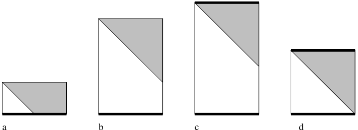
Figure 7: Penrose diagrams for $\kappa>0$ models. Thick lines indicate singularities. (a) Short big-bang geometry, (b) tall big-bang geometry, (c) tall re-collapsing geometry, (d) marginally tall re-collapsing geometry.

The family of big-bang solutions with $0<\kappa<2$ is easily seen to include both tall and short geometries, as indicated in figure 7. In the limit $\kappa\rightarrow 2$ the solution approaches the Einstein static universe and $\tilde{\eta}_{max}$ in (41) diverges logarithmically, leading to an arbitrarily tall Penrose diagram. On the other hand, $\tilde{\eta}_{max}$ goes to zero when $\kappa\rightarrow 0$ and the associated Penrose diagram becomes arbitrarily short. The $\kappa=0$ Penrose diagram in figure 6a may be obtained from the $\kappa>0$ diagrams by rescaling both axes in figure 7a by $1/\sqrt{k}$ before taking the $k\rightarrow 0$ limit. The Penrose diagrams for hyperbolic $\kappa<0$ big-bang geometries are the same as for the spatially flat case and are shown in figure 6.

For the re-collapsing big-bang solutions with $\kappa>2$, conformal time is cut off at the big crunch singularity. These geometries are nevertheless all tall. For $\kappa$ close to 2 they are very tall (figure 7c) as the lifetime of the universe diverges in the $\kappa\rightarrow 2^{+}$ limit, while for large $\kappa$ (figure 7d) they are marginally tall ($\tilde{\eta}_{max}\rightarrow\pi$) and we recover the behavior of closed cosmological models with $\Lambda=0$ where the spatial geometry becomes fully visible to a comoving observer at the big crunch.

The causal structure of the $\kappa>2$ bounce solutions (23) can be analyzed in a similar fashion. In this case we have $-\tilde{\eta}_{max}\leq\tilde{\eta}\leq\tilde{\eta}_{max}$ with

$$\tilde{\eta}_{max} = \sqrt{\kappa}\int_{0}^{\infty}{dx\over\sqrt{{\kappa\over 2}+\sqrt{{\kappa^{2}\over 4}-1}\cosh 2x}}$$ (42)

$$= 2\int_{0}^{1}{dy\over\sqrt{2y^{2}+\sqrt{1-{4\over\kappa^{2}}}(1+y^{4})}}\,.$$

The integral is clearly a decreasing function of $\kappa$, with $\tilde{\eta}_{max}\rightarrow{\pi\over 2}$ as $\kappa\rightarrow\infty$. This means that the bounce geometries are all ‘tall’, in agreement with a general result of Gao and Wald [24] regarding asymptotically de Sitter spacetimes. The bounces with $\kappa\rightarrow\infty$ are approaching de Sitter spacetime and are therefore only marginally tall but $\tilde{\eta}_{max}$ diverges as $\kappa\rightarrow 2^{+}$ and so the family of bounce solutions contains geometries with arbitrarily tall Penrose diagrams, see figure 8.

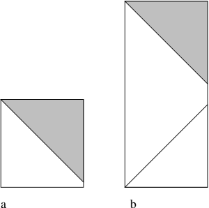
Figure 8: (a) Marginally tall bounce geometry, (b) very tall bounce geometry.

For $\kappa>0$ solutions the line element (33) determines the proper volume of the spatial geometry as a function of comoving time,

$$V(\tau)={2\pi^{2}\over\kappa^{3/2}}\,u(\tau)^{3}\left({3\over\Lambda}\right)^{3/2}\,,$$ (43)

in 3+1 spacetime dimensions (with a corresponding formula for the volume of $4{+}1$-dimensional dust universes). The minimum volume of a bounce universe occurs at $\tau=0$,

$$V_{min}=\left({1\over 2}+\sqrt{{1\over 4}-{1\over\kappa^{2}}}\right)^{3/2}2\pi^{2}\left({3\over\Lambda}\right)^{3/2}\,.$$ (44)

It is an increasing function of $\kappa$, which approaches the minimum spatial volume of de Sitter space in global coordinates for large $\kappa$, and varies over a relatively narrow range: $V_{min}(\kappa\rightarrow\infty)=V_{min}(dS)=2^{3/2}\,V_{min}(\kappa\rightarrow 2)$.

3.3 Dust models

We now turn our attention to models with matter in the form of pressureless dust. As mentioned previously, the $4{+}1$-dimensional case is identical the $3{+}1$-dimensional radiation models we have just discussed. For $3{+}1$-dimensional models with dust we do not have explicit analytic solutions at our disposal, except for the $\kappa=0$ model, but numerical results are in qualitative agreement with the picture obtained in 4+1 dimensions. In particular, 3+1-dimensional bounce geometries with dust are all tall, as are the re-collapsing big-bang geometries. The same numerical calculations apply to 2+1-dimensional models with radiation.

In section (2.4) we found explicit solutions for dust models in 2+1 dimensions. The conformal time of the bounce geometries (26) is given by

$$\tilde{\eta}(\tau) = \sqrt{\kappa\over\kappa-1}\int_{0}^{\tau}{dx\over\cosh{x}}$$ (45)

$$= \sqrt{\kappa\over\kappa-1}\left(2\arctan{(e^{\tau})}-{\pi\over 2}\right)\,.$$

The range is $-\tilde{\eta}_{max}<\tilde{\eta}<\tilde{\eta}_{max}$ with

$$\tilde{\eta}_{max}=\sqrt{\kappa\over\kappa-1}\,{\pi\over 2}\,.$$ (46)

As $\kappa$ is varied over its allowed range the bounce geometries go from being very tall as $\kappa\rightarrow 1^{+}$ to marginally tall in the $\kappa\rightarrow\infty$ pure de Sitter limit.

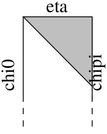
Figure 9: Big-bang geometry for dust in 2+1 dimensions, with $0<\kappa<1$.

So far the story is similar to the higher dimensional models but when it comes to the big-bang models (25) we find different behavior. Conformal time is logarithmically divergent as $\tau\rightarrow 0$ for these models,

$$\tilde{\eta}(\tau) = -\sqrt{|\kappa|\over 1-\kappa}\int_{\tau}^{\infty}{dx\over\sinh{x}}$$ (47)

$$= \sqrt{|\kappa|\over 1-\kappa}\log{\left({e^{\tau}-1\over e^{\tau}+1}\right)}\,.$$

The Penrose diagram for big-bang models with $0<\kappa<1$ is shown in figure 9. The dimensionless radial variable has finite range $0\leq\chi\leq\pi$, while the dimensionless conformal time ranges from $\tilde{\eta}\rightarrow-\infty$ at the initial singularity to $\tilde{\eta}=0$ in the asymptotic future. It follows that the entire spatial geometry is in the causal past of an observer at $\chi=0$ at any finite comoving time $\tau>0$. We note, however, that this strange property is derived from a classical solution but comes from a period of early evolution following an inital singularity where classical solutions have limited validity.

The big-bang geometry with $\kappa=0$ is an example of a spatially flat model with $\beta\geq 1$ (in fact $\beta=1$) and the Penrose diagram is shown in figure 6b. The same Penrose diagram applies to the hyperbolic $\kappa<0$ models and the same reservations apply concerning the physical relevance of such diagrams.

3.4 Negative pressure models

We close this section by analyzing the causal structure of the cosmological models with negative pressure matter introduced in section (2.5). Let us first consider the big-bang models (29) with $\kappa<0$. The initial expansion is linear in $\tau$, just as it was for dust models in 2+1 dimensions and the construction of the Penrose diagram is analogous. Conformal time is defined

$$\tilde{\eta}(\tau) = -\sqrt{-\kappa}\int_{\tau}^{\infty}{dx\over\sinh^{2}{x\over 2}+\sqrt{-\kappa}\sinh{x}}$$ (48)

$$= \log{\left({e^{\tau}-1\over e^{\tau}-b}\right)}\,,$$

with $b={1-2\sqrt{-\kappa}\over 1+2\sqrt{-\kappa}}$. The conformal time is logarithmically divergent as $\tau\rightarrow 0$ and the Penrose diagram of the classical geometry is identical to the one in figure 6b.

For $\kappa>0$ we have the bounce solutions (30) with conformal time given by

$$\tilde{\eta}(\tau) = \sqrt{\kappa}\int_{0}^{\tau}{dx\over\sqrt{\kappa+{1\over 4}}\cosh{x}-{1\over 2}}$$ (49)

$$= 2\left(\arctan{g(\tau)}-\arctan{g(0)}\right)\,,$$

where $g(\tau)=\sqrt{1+{1\over 4\kappa}}\,e^{\tau}-\sqrt{1\over 4\kappa}$. The range is $-\tilde{\eta}_{max}<\tilde{\eta}<\tilde{\eta}_{max}$ with

$$\tilde{\eta}_{max}=\pi-2\arctan{g(0)}.$$ (50)

Since $\tilde{\eta}_{max}>\pi/2$ for all $\kappa>0$ these bounce solutions are all tall. The limiting behavior is $\tilde{\eta}_{max}\rightarrow\pi/2$ as $\kappa\rightarrow\infty$, as appropriate for a bounce solution that approaches the de Sitter vacuum, and $\tilde{\eta}_{max}\rightarrow\pi$ as $\kappa\rightarrow 0$. The second limit is interesting in that a bounce geometry with $\tilde{\eta}_{max}\geq\pi$ is not only tall but ‘very tall’ in the terminology of [17]. Then an entire Cauchy surface lies in the causal past of a comoving observer at late times and also in the causal future of the same observer at an early enough time. For this Cauchy surface we can, for example, choose the spatial slice at $\tau=0$, which is also when the proper spatial volume of the bounce universe takes its minimum value,

$$V_{min}=\left(\sqrt{1+{1\over 4\kappa}}-\sqrt{1\over 4\kappa}\right)^{n}V_{min}(dS)\,,$$ (51)

where $V_{min}(dS)=a_{n}[n(n-1)/2\Lambda]^{n/2}$ is the minimum volume of the spatial slice of $n{+}1$-dimensional de Sitter spacetime in global coordinates. We note that the minimum volume of the bounce universe vanishes as $\kappa^{n}$ in the $\kappa\rightarrow 0$ limit.

We also have a $\kappa=0$ big-bang solution, which is a special case of (12) with $\beta=2$, and has infinite spatial volume at any $\tau>0$. The conformal time is linearly divergent as $\tau\rightarrow 0$, rather than the logarithmic divergence found for $\kappa<0$, but the Penrose diagram of the classical solution remains that of figure 6b.

4 Cosmological horizons

A finite maximal conformal time implies a cosmological event horizon for a comoving observer. This is, for example, evident in the Penrose diagram in figure 6a where there are regions of spacetime which can have no influence on an observer at $\chi=0$. The existence of a horizon has interesting implications for cosmological observations in an accelerating universe [25] and also motivates questions concerning holography and entropy bounds, which we address in section 6. The event horizon forms the boundary of the causal past of a comoving observer in the asymptotic future. It can therefore only be described from knowledge of the full future evolution of the cosmological model. The shaded regions in the various Penrose diagrams displayed in section 3 are outside the event horizon of an observer at $\chi=0$.

There is another notion of horizon which is based on local data. This is the apparent horizon, which is at the boundary of future trapped (or anti-trapped) spatial regions at any given cosmic time. In the de Sitter vacuum the apparent horizon coincides with the event horizon, but in an evolving geometry, which is future asymptotically de Sitter, the two will only agree in the far future.

4.1 The event horizon

Consider $n{+}1$ dimensional cosmological models that are future asymptotically de Sitter. The scale factor of these solutions grows exponentially at late times. In terms of our dimensionless variables the asymptotic rate of expansion is always the same,

$$u(\tau)\approx a\,e^{\tau}\,,$$ (52)

but subleading behavior, such as the constant $a$, in general depends on the number of dimensions, the equation of state, and the matter energy density.

The line element (33) implies that the event horizon of an observer at $\chi=0$ is the null surface

$$\chi_{eh}(\tau)=\tilde{\eta}_{max}-\tilde{\eta}(\tau)\,.$$ (53)

For a tall big-bang geometry with $\kappa>0$, for which $\tilde{\eta}_{max}-\tilde{\eta}_{min}>\pi$, the event horizon comes into existence at $\tau=\tau_{0}$, at which $\chi_{eh}(\tau_{0})=\pi$, while for a short $\kappa>0$ geometry, and also for all big-bang models with $\kappa\leq 0$, the event horizon forms at the initial singularity.

The proper area of the intersection of the event horizon with the spatial volume at comoving time $\tau$ is given by

$${\cal A}_{eh}(\tau)=a_{n-1}\left(|\kappa|^{-1/2}u(\tau)f(\chi_{eh}(\tau))\right)^{n-1}\left({n(n-1)\over 2\Lambda}\right)^{(n-1)/2}\,,$$ (54)

where $f(\chi)$ depends on the sign of $\kappa$ as in (34). The area starts out at zero when the horizon forms and then increases monotonically with time in all our models that are future asymptotically de Sitter. It is straightforward to show, using the asymptotic form (52), that

$$|\kappa|^{-1/2}u(\tau)f(\chi_{eh}(\tau))\rightarrow 1\qquad{\rm as}\qquad\tau\rightarrow\infty\,,$$ (55)

for all $a$. The limiting value of the horizon area is therefore independent of $\kappa$,

$$\lim_{\tau\rightarrow\infty}{\cal A}_{eh}(\tau)=a_{n-1}\left({n(n-1)\over 2\Lambda}\right)^{(n-1)/2}={\cal A}_{dS}\,.$$ (56)

As expected, the area approaches the area of the cosmological horizon in empty $n{+}1$-dimensional de Sitter spacetime with cosmological constant $\Lambda$. As time goes on in an accelerating universe the spatial region inside the event horizon occupies an ever smaller patch around $\chi=0$ in comoving coordinates and the global structure of the spatial geometry becomes irrelevant.

It is also easy to see, after appropriate rescaling of variables by powers of $k$, that the $\kappa\rightarrow 0$ limit of ${\cal A}_{eh}(\tau)$ is smooth and gives the same result as a direct $k=0$ calculation.

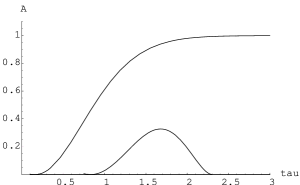
Figure 10: The area of the event horizon relative to the corresponding de Sitter horizon area, as a function of $\tau$ for ever-expanding and re-collapsing big-bang geometries.

Now consider the bounce solutions which are both past and future asymptotically de Sitter. The definition of the event horizon in equation (53) continues to hold, and since these geometries are all tall the event horizon comes into existence at $\chi_{eh}(\tau_{0})=\pi$ at some finite comoving time $\tau_{0}$. The area starts out at zero, then increases with time until it approaches ${\cal A}_{dS}$ at late times. Note that the area of the event horizon grows with time even when the horizon forms at $\tau_{0}<0$ in the contracting phase of the bounce evolution.

Finally, we come to the big-bang solutions which re-collapse in a big-crunch singularity. In this case, we can define the event horizon of an observer at $\chi=0$ as in equation (53) with $\tilde{\eta}_{max}$ taken as the conformal time at the final singularity. With this definition the event horizon starts with zero area at $\chi=\pi$ at some time after the big bang. The horizon area grows initially but as the geometry collapses towards the big crunch the area shrinks again and goes to zero at the final singularity. Figure 10 shows how the ratio ${\cal A}_{eh}(\tau)/{\cal A}_{dS}$ evolves for two big-bang models, one that accelerates forever and another that re-collapses.

4.2 The apparent horizon

Consider spherical $n{-}1$ surfaces centered on an observer at $\chi=0$ in one of our $n{+}1$-dimensional cosmological models. Such a surface is uniquely characterized by a value of $\chi$ and a conformal time $\tilde{\eta}$. A radial null ray is orthogonal to such a spherical surface. It is future (past) directed if $\tilde{\eta}$ increases (decreases) along the ray away from the sphere and outgoing (incoming) if $\chi$ increases (decreases). Thus there are four families of null rays orthogonal to each sphere.

Let $\lambda$ be the affine parameter of null rays in one of the null directions orthogonal to a given spherical surface. By a linear transformation of $\lambda$ on each null ray we can set $\lambda=0$ where this family of null rays intersects our surface and also ensure that we advance at the same rate along all the null rays at $\lambda=0$. The surface intersected by our null rays at infinitesimal parameter distance $d\lambda$ is then also spherical. The expansion $\theta$ is then defined in terms of the rate of change of the proper area (35) of the surface intersected by the family of null rays,

$$\theta(\lambda)={1\over{\cal A}}\,{d{\cal A}\over d\lambda}\,.$$ (57)

By a more general construction the expansion can be defined locally on any $n{-}1$ surface [20], but for the purposes of the present paper the above definition involving spherical surfaces will be sufficient.

If a family of null rays orthogonal to a given spherical surface has non-positive expansion, $\theta(\lambda)\leq 0$, it is referred to as a light-sheet of that surface. At least two of the four families of null rays orthogonal to a surface will satisfy this condition. The light-sheet extends along the family of null rays until positive expansion is encountered, in which case it terminates. Light sheets play a key role in the covariant entropy bound [16] which we will apply to some of our cosmological models in section 6.

In a normal region of spacetime outgoing (incoming) future directed null rays orthogonal to a surface have positive (negative) expansion. If both future directed families of null rays have negative expansion, i.e. are light-sheets, the surface is said to be in a future trapped region. This occurs, for example, inside the event horizon of a Schwarzschild black hole. If, on the other hand, both future directed families of null rays have positive expansion, i.e. the past directed families are light-sheets, the spherical surface is in a future anti-trapped region. An example of this behavior is provided by spherical surfaces outside the cosmological event horizon of an observer in de Sitter spacetime.

The boundary between normal and trapped (or anti-trapped) regions is called an apparent horizon. At least one pair out of the four families of null rays has vanishing expansion there. In de Sitter spacetime, for example, there is an apparent horizon which coincides with the de Sitter event horizon. There is no reason to expect the two types of horizons to coincide in more general, evolving geometries.

In our cosmological solutions we can, for example, identify the affine parameter with the conformal time itself, $\lambda=\pm(\tilde{\eta}-\tilde{\eta}_{0})$, where $\tilde{\eta}_{0}$ is the conformal time coordinate of our spherical surface and the sign depends on whether the family of null rays is future or past directed. Null rays that are orthogonal to the surface are radial and satisfy $d\chi/d\lambda=\pm 1$, with the sign indicating whether they are outgoing or incoming. For future directed null rays the expansion is thus given by

$$\theta = (n-1)\left({1\over u}{du\over d\tilde{\eta}}\pm{1\over f}{df\over d\chi}\right)$$ (58)

$$= (n-1)\left({1\over\sqrt{|\kappa|}}{du\over d\tau}\pm{1\over f}{df\over d\chi}\right)\,,$$

with $f(\chi)$ given in (34). An apparent horizon is then located wherever

$${1\over|\kappa|}\left({du\over d\tau}\right)^{2}={1\over f^{2}}\left({df\over d\chi}\right)^{2}\,.$$ (59)

In a universe undergoing accelerated expansion the apparent horizon separates a normal region at $0\leq\chi<\chi_{ah}$ and a future anti-trapped region at $\chi>\chi_{ah}$. When $\kappa>0$ we have $f(\chi)=\sin{\chi}$ and the apparent horizon condition (59) can be rewritten as

$$\sin{(\chi_{ah}(\tau))}=\left(1+{1\over\kappa}\left(du/d\tau\right)^{2}\right)^{-1/2}\,.$$ (60)

The area of the apparent horizon is then given by

$${\cal A}_{ah}(\tau) = a_{n{-}1}\left(\kappa^{-1/2}u(\tau)\sin{(\chi_{ah}(\tau))}\right)^{n-1}\left({n(n{-}1)\over 2\Lambda}\right)^{(n-1)/2}$$ (61)

$$= \left({u^{2}\over\kappa+(du/d\tau)^{2}}\right)^{(n-1)/2}{\cal A}_{dS}\,,$$

where ${\cal A}_{dS}$ is the area of the corresponding de Sitter event horizon. By using the evolution equation (9) we can eliminate the derivative of the scale factor to obtain

$${\cal A}_{ah}(\tau)=\left(1+u^{-(1+\alpha)n}\right)^{-(n-1)/2}{\cal A}_{dS}\,.$$ (62)

In the corresponding calculations for $\kappa<0$ solutions, equation (60) is replaced by

$$\sinh{(\chi_{ah}(\tau))}=\left(-1+{1\over|\kappa|}\left(du/d\tau\right)^{2}\right)^{-1/2}\,,$$ (63)

and for the spatially flat case one has $r_{ah}(t)=(dR/dt)^{-1}$. In all cases the end result in (61) and (62) for the area of the apparent horizon is the same. We note that ${\cal A}_{ah}<{\cal A}_{dS}$ for all physical values of the scale factor and that ${\cal A}_{ah}$ tends towards ${\cal A}_{dS}$ as $u\rightarrow\infty$.

An interesting feature of $\kappa>0$ solutions, whose spatial sections are $n$-spheres, is that the apparent horizon condition (60) has two solutions that are equidistant from the equator. In an expanding $\kappa>0$ universe the apparent horizon in the northern hemisphere is the boundary between the normal region near the observer at $\chi=0$ and an anti-trapped region where both future directed families of null rays have positive expansion. Beyond the other apparent horizon, which is in the southern hemisphere, we are again in a normal region where one future directed family of null rays has negative expansion and the other positive. It is, however, the null rays that are outgoing with respect to the observer at $\chi=0$ that have negative expansion.

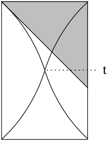
Figure 11: Penrose diagram for a bounce solution with the event horizon and both apparent horzions indicated.

Now consider bounce solutions. At the minimal scale factor we have $du/d\tau=0$. It then follows from equation (60) that both apparent horizons must be at the equator at that point. The location of the two apparent horizons in comoving coordinates can be traced throughout the bounce evolution as follows. In the asymptotic past a pair of apparent horizons emerges from the north and south poles and in the contracting $\tau<0$ phase the two polar regions are normal while the region between the apparent horizons is future trapped. As the scale factor approaches its minimum value the trapped region contracts to a narrow band around the equator, which then vanishes at $\tau=0$ when the two apparent horizons meet. In the expanding $\tau>0$ phase the apparent horizons separate again but now the equatorial region has become anti-trapped. In the asymptotic future the two apparent horizons approach the north and south poles.

The cosmological event horizon in a future asymptotically de Sitter spacetime is an example of a family of null rays that are orthogonal to transverse $n{-}1$ spheres. The area of the transverse sphere intersected by the event horizon increases with comoving time. It follows that the past directed null rays along the event horizon form a light-sheet and also that $\chi_{eh}(\tau)\geq\chi_{ah}(\tau)$, i.e. the event horizon is always outside the apparent horizon. In a $\kappa>0$ geometry this statement refers to the apparent horizon that is closer to $\chi=0$. The event horizon may or may not be outside the other apparent horizon at $\chi=\pi-\chi_{ah}(\tau)$. Note, furthermore, that an event horizon that forms at $\chi>\pi/2$ in a $\kappa>0$ geometry may have less area than the apparent horizon early on, despite being outside the apparent horizon. To give an example, figure 11 shows the location of the event horizon and both apparent horizons in the Penrose diagram for a bounce geometry.

5 Cosmological evolution as renormalization group flow

The $n{+}1$-dimensional de Sitter vacuum is conjectured to be dual to an $n$-dimensional conformal field theory [9]. The case is strongest for three-dimensional spacetime where the dual field theory is two-dimensional. An analysis of the asymptotic symmetry generators of three-dimensional de Sitter spacetime [9] revealed a conformal algebra with central charge

$$c={3\over 2G\Lambda}\,.$$ (64)

On dimensional grounds, the expected generalization to higher dimensions is

$$c\sim{1\over G\Lambda^{(n-1)/2}}\,,$$ (65)

up to an undetermined constant of proportionality.

More generally in this context, cosmological evolution in a model which is future asymptotic to de Sitter spacetime represents a reverse renormalization group flow on the dual field theory side [10, 11]. A candidate c-function was proposed, that could be evaluated on the gravity side and shown to decrease towards the infrared along the renormalization group flow, provided the matter in the cosmological model satisfies the weak energy condition, i.e. $\rho\geq-P$ and $\rho>0$. The original papers [9, 11] considered spatially flat cosmological models with $k=0$ but their c-function was subsequently generalized [17] so as to apply to $k\neq 0$ models as well.

We take a different route to arrive at the same c-function as [17]. Our starting point is the observation that the central charge (65) of the $n$-dimensional fixed point theory is proportional to the area of the event horizon in Planck units in the corresponding $n{+}1$-dimensional de Sitter spacetime. We wish to identify a c-function that reduces to this central charge at the ultraviolet fixed point of the renormalization group flow and decreases along the flow towards the infrared, i.e. increases as the cosmological scale factor grows and approaches de Sitter expansion. The evolving horizon area is then a natural candidate for a c-function, but we have a choice to make between the area of the event horizon and that of the apparent horizon. At least two factors count against choosing the the area of the event horizon. One is that global information about the spacetime geometry is required in order to determine the location of the event horizon, and therefore also its area, at a given comoving time. The other is the related fact that for some geometries there are times when the event horizon has yet to come into existence. The apparent horizon, on the other hand, is defined by local data on any spatial slice and it exists at all times in all our cosmological models.

We therefore define the c-function associated with an asymptotically de Sitter spacetime to be (proportional to) the area of the cosmological apparent horizon in Planck units,

$$c\sim{{\cal A}_{ah}\over G}\,.$$ (66)

With this definition we have a prescription for evaluating the c-function on any constant time slice, and the c-theorem becomes a geometric statement about the increase in area of the apparent cosmological horizon in an accelerating universe.

For any metric of Robertson-Walker form (1), our definition gives

$$c\sim\left({u^{2}\over\kappa+(du/d\tau)^{2}}\right)^{(n-1)/2}\frac{{\cal A}_{dS}}{G}$$ (67)

which is the same c-function as the one advocated in [17]. Our proposal can be viewed as providing a geometric interpretation of their c-function. The definition of an apparent horizon can be extended to anisotropic cosmological models and we expect our geometric approach to remain useful for such models as well.

By using the evolution equation (9) the c-function for our models may be written,

$$c\sim\frac{{\cal A}_{dS}}{\left(1+u^{-(1+\alpha)n}\right)^{(n-1)/2}G}.$$ (68)

This expression makes manifest the UV/IR correspondence of the proposed dS/cft duality. The c-function only depends on the overall scale $u$ of the geometry and $c$ decreases as we move to smaller scales on the gravity side, which corresponds to flowing to the infrared in the dual field theory.

This means, for example, in a big-bang model approaching de Sitter acceleration in the future that it is the reverse of the cosmological evolution that corresponds to renormalization group trajectories starting at an ultraviolet fixed point theory. The c-function then decreases monotonically along the flow towards the infrared but it is less clear how to interpret the endpoint of the flow where the c-function goes to zero at a big-bang singularity on the gravitational side. Evolution forward in time corresponds to renormalization group flow in a big-crunch model that is past asymptotically de Sitter, with the c-function again vanishing at the singular endpoint. Re-collapsing big-bang geometries are singular at both ends and do not lend themselves to straightforward interpretation as renormalization group flow. For bounce solutions, the gravitational evolution is non-singular everywhere but instead the scale factor is not a monotonic function of comoving time. If we follow the cosmological evolution backwards (or forwards) in time the scale factor eventually stops decreasing and begins to grow, and it is clear that the full time history cannot represent a single renormalization group flow in the usual sense. In [17], where analogous bounce geometries were considered, it is suggested to view them as matching two separate renormalization group flows arriving at the same effective field theory from opposite time directions.

6 Holography and entropy

We end the paper with an application of the holographic principle [26, 27], in the form of the covariant entropy bound [16], in the context of these cosmological models. The basic idea is to use the fact that the cosmological event horizon of a comoving observer in a future asymptotically de Sitter spacetime provides a past directed light-sheet for any transverse $n{-}1$-sphere it intersects. We will apply the covariant entropy bound to the light-sheet of such a transverse sphere at asymptotically late time. In this case the area approaches the area of the corresponding de Sitter horizon ${\cal A}_{dS}$, and we can compare the total entropy that crosses the light-sheet to ${\cal A}_{dS}/4$. We will make the assumption that entropy in a cosmological spacetime may be described by a local ‘entropy fluid’. This cannot be correct in any fundamental sense, given that entropy is not a local quantity, but it is an approximation often made in cosmology.

Recall that the area of the de Sitter horizon in (56) involves an inverse power of $\Lambda$ and therefore becomes large in the limit of small $\Lambda$. On the other hand, for models with $\kappa\geq 0$ the volume enclosed by this area grows even faster with vanishing $\Lambda$ and one might worry that this could lead to a violation of the entropy bound for sufficiently small values of the cosmological constant. As we will see below, such a conflict only arises in models with somewhat exotic matter content and there it can be traced to the failure of classical solutions to correctly describe the physics close to the initial singularity.

Let us first apply these ideas to cosmological models with matter in the form of radiation, under the assumption that the cosmological expansion is adiabatic. In this case, no violation of the entropy bound is found but the exercise serves to illustrate the argument. A simple relationship can be established between the proper entropy density $s$ and the energy density $\rho$ at a given comoving time. Both these quantities are related to the temperature $T$ of the gas of radiation,

$$\rho\sim T^{n+1}\,,\qquad s\sim T^{n}\,.$$ (69)

The energy density can in turn be related to the cosmological constant and the scale factor $u(\tau)$ through equation (7), leading to

$$s\sim\rho^{n/(n+1)}\sim u^{-n}\left({\Lambda\over G}\right)^{n/(n+1)}\,.$$ (70)

The dependence on the scale factor reflects the fact that the entropy density is diluted by the cosmological expansion, while the comoving entropy density $\tilde{s}\equiv u^{n}\,s$ remains constant throughout the evolution.

The next step is to obtain the total entropy that crosses the event horizon. This is given by the product of the comoving entropy density and the largest comoving volume enclosed by the event horizon, which occurs whenever the event horizon comes into existence. For concreteness, let us consider a spatially flat model for which the event horizon of an observer at $r=0$ meets the initial singularity at $r=\eta_{max}$, as is evident from figure 6a.

The maximal conformal time given in equation (37) gives

$$\tilde{V}_{max}\sim\Lambda^{-n/2}$$ (71)

for the maximal comoving volume enclosed by the event horizon. The total entropy that passes through the light-sheet is thus

$$S=\tilde{s}\,\tilde{V}_{max}\sim G^{-\frac{n}{n+1}}\Lambda^{-\frac{n(n-1)}{n(n+1)}}.$$ (72)

The ratio between this entropy and the horizon area at late times in Planck units is given by

$$\frac{S}{{\cal A}_{dS}/G}\sim G^{\frac{1}{n+1}}\Lambda^{\frac{1}{2}\left(\frac{n-1}{n+1}\right)}.$$ (73)

So we see that this ratio actually vanishes in the limit of small $\Lambda$ and the covariant entropy bound is far from being saturated, let alone violated, in this limit.

The story is different when we consider spatially flat models with an equation of state such that $\beta\geq 1$ in (12). Models that exhibit this behavior include the $\kappa=0$ solution for dust in 2+1 dimensions, which has $\beta=1$, and the negative pressure models in section 2.5, which have $\beta=2$. The relevant Penrose diagram is now the one in figure 6b rather than figure 6a. The covariant entropy bound is violated because an infinite amount of entropy will cross the event horizon of any comoving observer while the horizon area remains bounded by the area of the corresponding de Sitter horizon. This conclusion could be avoided if the expansion of the past directed null rays along the event horizon were to become positive at some time in the past, in which case the light-sheet would terminate and the total entropy passing through it would be finite. This cannot happen, however, as long as the area of the event horizon increases with time. A simple calculation for the $\kappa=0$ negative pressure models, for example, shows that

$${\cal A}_{eh}(\tau)=(1-e^{-\tau}){\cal A}_{dS},$$ (74)

which clearly grows monotonically with $\tau$. The Penrose diagram in figure 6b also applies to hyperbolic models with $\kappa<0$ and $\beta\geq 1$ and the above argument may be adapted to arrive at a violation of the covariant entropy bound in these models as well.

How seriously are we to take this violation of the covariant entropy bound? The matter considered here has zero or negative pressure but does nevertheless obey the dominant energy condition. The corresponding cosmological models are perfectly good classical solutions of Einstein gravity but a proof of the covariant entropy bound has been given in classical gravity, under certain assumptions about properties of the entropy fluid in spacetime [28]. At first sight, our results appear to contradict that proof but a closer look reveals that it is not so. The source of the conflict with the covariant entropy bound lies in the failure of conformal time to converge at the initial singularity in these models. As a result the expansion starts off so slowly that an infinite comoving volume is visible in the causal past of any observer at finite $\tau>0$. The geometry is singular at $\tau=0$ and a straightforward calculation reveals that at very early times these big-bang solutions fail to meet the assumptions made in the proof of the covariant entropy bound in [28]. Such early times are, however, beyond the reach of classical gravity and should not be included in a classical cosmological model [23]. By adapting arguments made in [29] and [23] to models with postitive $\Lambda$, one can show that if the covariant entropy bound is assumed to be satisfied at the Planck time it will not be violated at later times. We therefore conclude that there is no conflict with the covariant entropy bound after all in any of our cosmological models but that in some cases the bound requires quantum effects to modify the early causal structure from that of classical big-bang solutions, changing Penrose diagrams of the form shown in figure 6b to diagrams as shown in figure 6a.

- [1] S. Perlmutter et al., Astrophys. J. 483 (1997) 565, [astro-ph/9608192]. S. Perlmutter et al., Nature 391 (1998) 51, [astro-ph/9712212]. A.G. Riess et al., Astroph. J. 116 (1998) 1009, [astro-ph/9805201]. N.A. Bachall, J.P. Ostriker, S. Perlmutter, and P. Steinhardt, Science 284 (1999) 1481, [astro-ph/9906463].
- [2] C.M. Hull, J. High Energy Phys. 9807 (1998) 021, [hep-th/9806146].
- [3] J. Maldacena and A. Strominger, J. High Energy Phys. 9802 (1998) 014, [gr-qc/9801096]. S. Hawking, J. Maldacena and A. Strominger, J. High Energy Phys. 0105 (2001) 001, [hep-th/0002145].
- [4] T. Banks, [hep-th/0007146].
- [5] R. Bousso, J. High Energy Phys. 0011 (2000) 038, [hep-th/0010252]; ibid 0104 (2001) 035, [hep-th/0012052].
- [6] T. Banks and W. Fischler, [hep-th/0102077].
- [7] V. Balasubramanian, P. Horova and D. Minic, J. High Energy Phys. 0105 (2001) 043, [hep-th/0103171].
- [8] E. Witten, [hep-th/0106109].
- [9] A. Strominger, J. High Energy Phys. 0110 (2001) 034, [hep-th/0106113].
- [10] A. Strominger, J. High Energy Phys. 0111 (2001) 049, [hep-th/0110087].
- [11] V. Balasubramanian, J. de Boer, and D. Minic, [hep-th/0110108].
- [12] For a review, see O. Aharony et al., Phys. Rept. 323 (2000) 183, [hep-th/9905111].
- [13] G. Gibbons and S.W. Hawking, Phys. Rev. D 15 (1977) 2738.
- [14] W. Fischler, Taking de Sitter Seriously, conference talk at Role of Scaling Laws in Physics and Biology, Santa Fe, December 2000.
- [15] L. Dyson, J. Lindesay, and L. Susskind, [hep-th/0202163].
- [16] R. Bousso, J. High Energy Phys. 07 (1999) 004, [hep-th/9905177]. R. Bousso, J. High Energy Phys. 06 (1999) 028, [hep-th/9906022]. For a review see R. Bousso, [hep-th/0203101].
- [17] F. Leblond, D. Marolf, and R.C. Myers, [hep-th/0202094].
- [18] A.J.M. Medved, [hep-th/0203191].
- [19] C.W. Misner, K.S. Thorne, and J.A. Wheeler, Gravitation, W.H. Freeman and Company, 1973.
- [20] S.W. Hawking and G.F.R. Ellis, Large Scale Structure of Spacetime, Cambridge University Press, 1973.
- [21] P.J.E. Peebles, Principles of Physical Cosmology, Princeton University Press, 1993.
- [22] C. Wetterich, Nucl. Phys. B 302 (1988) 668. B. Ratra and P.J.E. Peebles, Phys. Rev. D 37 (1988) 3406. R.R. Caldwell, R. Dave, and P.J. Steinhardt, Phys. Rev. Lett. 80 (1998) 1582.
- [23] N. Kaloper and A. Linde, Phys. Rev. D 60 (1999) 103509, [hep-th/9904120].
- [24] S. Gao and R. Wald, Phys. Rev. D 64 (2001) 084020, [gr-qc/0106071].
- [25] E.H. Gudmundsson and G. Björnsson, Astrophys. J. 565 (2002) 1, [astro-ph/0105547]. A. Loeb, Phys. Rev. D 65 (2002) 047301, [astro-ph/0107568].
- [26] G. ’t Hooft, [gr-qc/9310026].
- [27] L. Susskind, J. Math. Phys. 36 (1995) 6377, [hep-th/9409089].
- [28] E. Flanagan, D. Marolf and R.W. Wald, Phys. Rev. D 62 (2000) 084035, [hep-th/9908070].
- [29] W. Fischler and L. Susskind, [hep-th/9806039].