KIAS-P02016

hep-th/0204055

On Decoupling of Massless Modes
in NCOS Theories

Seungjoon Hyun^a, Sangmin Lee^b,c and Hyeonjoon Shin^b,c

^aInstitute of Physics and Applied Physics, Yonsei University, Seoul 120-749, Korea

^bBK 21 Physics Research Division and Institute of Basic Science

Sungkyunkwan University, Suwon 440-746, Korea

^cSchool of Physics, Korea Institute for Advanced Study, Seoul 130-012, Korea

Abstract

We revisit the decoupling phenomenon of massless modes in the noncommutative open string (NCOS) theories. We check the decoupling by explicit computation in (2+1) or higher dimensional NCOS theories and recapitulate the validity of the decoupling to all orders in perturbation theory.

1 Introduction

Noncommutative open string (NCOS) theories are defined by a scaling limit in which one takes an electric field on a brane to its critical value and at the same time scale $g_{s}$ and $\alpha^{\prime}$ appropriately so that the closed strings decouple and the open strings experience maximal noncommutativity in the electric direction [1, 2, 3, 4]. Their properties including S-duality and T-duality have been studied extensively [5]-[18].

It is of great interest to compare the dynamics of NCOS theories and their S-duals, but our limited understanding of the strong coupling dynamics allows only a few explicit checks. One such example is the decoupling phenomenon of massless modes in NCOS theories [5]. The authors of [5] observed that the S-dual super-Yang-Mills theories, in (1+1) or (3+1) dimensions for example, contain massless $U(1)$ fields which are free and decouple from the rest of the theory when their momenta have components only in the electric directions. S-duality implies then that the massless modes of NCOS theories also should be free. They showed that this is indeed the case by computing some amplitudes explicitly and also by giving a general argument based on holomorphy of world-sheet correlators. Subsequently, Ref. [11] gave more details of decoupling of the (1+1) dimensional NCOS and Ref. [14] generalized the holomorphy argument to prove that vanishing of the relevant amplitudes is exact to all order in perturbation theory.

So far, explicit computations have been limited to (1+1) dimensional NCOS. In the present work, we compute the amplitudes in (2+1) or higher dimensional NCOS theories and check that the decoupling phenomenon remains to be valid in higher dimensions. We also review the proof of the decoupling to all order given in [14] from a slightly different point of view.

2 Explicit Computation

Higher dimensional NCOS theories are more complicated than the (1+1)-dimensional one in two ways. First, the string modes can carry momentum in the non-electric directions. Second, the massless spectrum contains not only the transverse scalars but also gauge bosons. The goal of this section is to confirm by explicit computation that the decoupling phenomenon holds for arbitrary world-volume dimensions.

As a warm-up exercise, we first compute the amplitudes in the bosonic theory. We will see that they share all the essential features of decoupling with the superstring theory.

2.1 Bosonic String

Following [5, 11], we check the amplitudes involving massless modes and tachyons. The vertex operators are given by

$$V_{T} = G_{o}e^{ip\cdot X},$$

$$V_{\phi} = \frac{G_{o}}{\sqrt{\alpha^{\prime}_{e}}}\zeta_{i}\partial X^{i}e^{ip\cdot X},$$

$$V_{A} = \frac{G_{o}}{\sqrt{\alpha^{\prime}_{e}}}e_{\alpha}\partial X^{\alpha}e^{ip\cdot X},$$ (1)

where the scalars represent the transverse fluctuation of the world-volume ($\zeta_{i}$) and the gauge bosons are polarized along the world-volume ($e_{\alpha}$). The world-sheet correlators are

$$\langle X^{\alpha}(y)X^{\beta}(y^{\prime})\rangle = -2\alpha^{\prime}_{e}\eta^{\alpha\beta}\ln|y-y^{\prime}|+\frac{i}{2}\theta\epsilon^{\alpha\beta}{\rm sign}(y-y^{\prime}),$$

$$\langle\partial X^{i}(z)\partial X^{j}(z^{\prime})\rangle = -\frac{\alpha^{\prime}_{e}}{2}\frac{\eta^{ij}}{(z-z^{\prime})^{2}},$$ (2)

where $\alpha=0,\cdots,p$ and $i=p+1,\cdots,25$. $\epsilon^{01}=-\epsilon^{10}=1,\epsilon^{\alpha\beta}=0$ otherwise and $\theta=2\pi\alpha^{\prime}_{e}E$. In the NCOS limit, $E\rightarrow 1$ and hence $\theta\rightarrow 2\pi\alpha^{\prime}_{e}$. We introduce the dimensionless Mandelstam variables,

$$s = -\alpha^{\prime}_{e}(p_{1}+p_{2})^{2},$$

$$t = -\alpha^{\prime}_{e}(p_{1}+p_{4})^{2},$$

$$u = -\alpha^{\prime}_{e}(p_{1}+p_{3})^{2}.$$ (3)

Noncommutativity gives rise to phase factors. To each of the three inequivalent cyclic ordering, we associate a phase factor in the following way ($p\times q=\theta\epsilon^{\alpha\beta}p_{\alpha}q_{\beta}$),

$$\gamma_{1} = \cos\left[\frac{1}{2}(p_{1}\times p_{4}+p_{2}\times p_{3})\right],$$

$$\gamma_{2} = \cos\left[\frac{1}{2}(p_{1}\times p_{2}+p_{3}\times p_{4})\right],$$

$$\gamma_{3} = \cos\left[\frac{1}{2}(p_{1}\times p_{3}-p_{2}\times p_{4})\right].$$ (4)

The simplest amplitude of our interest is the scattering of a scalar off a tachyon. For obvious reasons, the result is formally the same as the (1+1)-dimensional answer given in [5, 11]. The transverse scalars are taken to have momenta $p_{1}$ and $p_{4}$ and polarization tensors $\zeta$ an $\zeta^{\prime}$, respectively, while tachyons have $p_{2}$ and $p_{3}$. Then the four-point scattering amplitude ${\cal A}_{\phi\phi TT}$ is given by

$${\cal A}_{\phi\phi TT}=-\frac{G_{o}^{2}}{\alpha^{\prime}_{e}}\zeta\cdot\zeta^{\prime}\left[B(-1-t,-u)\gamma_{1}+B(-1-t,-s)\gamma_{2}+B(-u,-s)\gamma_{3}\right]~{},$$ (5)

where $B(a,b)$ is the beta function and Mandelstam variables satisfy $s+t+u=-2$. It is convenient to rewrite this amplitude by using an identity for the gamma function, $\Gamma(z)\Gamma(1-z)=\pi/\sin(\pi z)~{}.$ The right hand side of Eq. (5) then becomes

$$-\frac{G_{o}^{2}}{\alpha^{\prime}_{e}}\zeta\cdot\zeta^{\prime}\frac{B(-1-t,-s)}{\sin(\pi u)}\Phi_{-}~{}.$$ (6)

Here we have defined $\Phi_{\pm}$ as

$$\Phi_{\pm}\equiv\sin(\pi s)\gamma_{1}+\sin(\pi u)\gamma_{2}\pm\sin(\pi t)\gamma_{3}~{}.$$ (7)

The factors $\Phi_{\pm}$, which combine the $\gamma$ factors due to the space-time noncommutativity and sine functions of Mandelstam variables, are crucial for showing the decoupling of massless modes from the rest of the NCOS modes. Other amplitudes involving massless modes also turn out to contain the factors $\Phi_{\pm}$. Since higher dimensional NCOS theories have dynamical gauge fields in addition to the transverse scalars, we still need to compute ${\cal A}_{\phi\phi\phi\phi}$, ${\cal A}_{AA\phi\phi}$, ${\cal A}_{AATT}$, ${\cal A}_{AAAA}$. The standard recipe for computing the amplitudes gives

1. Four scalars with momenta $p_{n}$ and polarizations $\zeta_{n}$ ($n=1,...,4$) :

   $${\cal A}_{\phi\phi\phi\phi} = \frac{G_{o}^{2}}{2\alpha^{\prime}_{e}}\left[\zeta_{1}\cdot\zeta_{2}\zeta_{3}\cdot\zeta_{4}\frac{B(1-t,1-u)}{\sin(\pi s)}+\zeta_{1}\cdot\zeta_{3}\zeta_{2}\cdot\zeta_{4}\frac{B(1-t,1-s)}{\sin(\pi u)}\right.$$ (8)

   $$\hskip 19.91692pt\left.+\zeta_{1}\cdot\zeta_{4}\zeta_{2}\cdot\zeta_{3}\frac{B(1-s,1-u)}{\sin(\pi t)}\right]\Phi_{+}~{}$$

2. Two gauge bosons with $(p_{1},e)$ and $(p_{4},e^{\prime})$, and two transverse scalars ($p_{2},\zeta)$ and $(p_{3},\zeta^{\prime})$ :

   $${\cal A}_{AA\phi\phi} = \frac{G_{o}^{2}}{2\alpha^{\prime}_{e}}\frac{\zeta\cdot\zeta^{\prime}}{\sin(\pi t)}$$ (9)

   $$\times \bigg{\{}\bigg{[}e\cdot e^{\prime}-2\alpha^{\prime}_{e}(e\cdot p_{2}e^{\prime}\cdot p_{2}+e\cdot p_{3}e^{\prime}\cdot p_{3})\bigg{]}B(1-s,1-u)$$

   $$+2\alpha^{\prime}_{e}\Big{[}e\cdot p_{2}e^{\prime}\cdot p_{3}B(2-u,-s)+e\cdot p_{3}e^{\prime}\cdot p_{2}B(2-s,-u)\Big{]}\bigg{\}}\Phi_{+}$$

3. Two gauge bosons with $(p_{1},e)$ and $(p_{4},e^{\prime})$ and two tachyons :

   $${\cal A}_{AATT} = \frac{G_{o}^{2}}{\alpha^{\prime}_{e}}\frac{1}{\sin(\pi t)}$$ (10)

   $$\times \bigg{\{}2\alpha^{\prime}_{e}\Big{[}e\cdot p_{2}e^{\prime}\cdot p_{3}B(1-u,-1-s)+e\cdot p_{3}e^{\prime}\cdot p_{2}B(1-s,-1-u)\Big{]}$$

   $$+\bigg{[}e\cdot e^{\prime}-2\alpha^{\prime}_{e}(e\cdot p_{2}e^{\prime}\cdot p_{2}+e\cdot p_{3}e^{\prime}\cdot p_{3})\bigg{]}B(-s,-u)\bigg{\}}\Phi_{-}$$

The expression for ${\cal A}_{AAAA}$ is more complicated. For our purposes, it suffices to note that it is proportional to $\Phi_{+}$. We observe that the appearance of the factors $\Phi_{\pm}$ is universal in the sense that the scattering amplitudes between massless states among themselves are always proportional to $\Phi_{+}$ and the ones between massless modes and massive modes are proportional to $\Phi_{-}$. In order to check the vanishing of the amplitude in the NCOS limit, it is sufficient to show that these factors vanish.

We show the vanishing of $\Phi_{-}$ first. There are three types of physical processes to consider: (a) Pair annihilation of massless particles and a subsequent pair creation of massive ones (b) Forward scattering of a massless particle off a massive one (c) Backward scattering. Our choice of center of mass momenta and the resulting phase factors are summarized in the following table.

	Pair annihilation	Forward scattering	Backward scattering
$p_{1}$	$(p,p,\vec{0})$	$(p,p,\vec{0})$	$(p,p,\vec{0})$
$p_{4}$	$(p,-p,\vec{0})$	$-(p,p,\vec{0})$	$-(p,-p,\vec{0})$
$p_{2}$	$-(p,q,\vec{k})$	$(e,-p,\vec{k})$	$(e,-p,\vec{0})$
$p_{3}$	$-(p,-q,-\vec{k})$	$-(e,-p,\vec{k})$	$-(e,p,\vec{0})$
$\gamma_{1}$	$\cos(\pi E(u+1))$	1	$\cos(\pi E(u+1))$
$\gamma_{2}$	$\cos(\pi E(s+1))$	1	$\cos(\pi E(s+1))$
$\gamma_{3}$	1	$\cos(\pi E(s+1))$	1

For instance, in the case of pair annihilation,

$$\Phi_{-}=\sin(\pi s)\cos\left(\pi E(u+1)\right)+\sin(\pi u)\cos\left(\pi E(s+1)\right)-\sin(\pi t),$$ (11)

which vanishes in the NCOS limit ($E\rightarrow 1$) due to the fact that $s+t+u=-2$. The backward scattering is shown to vanish in the same way. Note that the forward scattering vanishes even before taking the NCOS limit.

The vanishing of $\Phi_{+}$ can be verified similarly. The only change from the previous case is that the mass-shell condition is different. If we replace $(u+1)$ by $u$ and $(s+1)$ by $s$ in the phase factors $\gamma_{1,2,3}$, the above table becomes valid for the case at hand. This replacement together with the condition that $s+t+u=0$ for massless modes make sure that $\Phi_{+}$ also vanishes.

2.2 Superstring

Strictly speaking, the NCOS theories and their S-duals are well-defined only in Type II superstring theories. However, as we saw in the previous subsection, the reason for the decoupling is mainly kinematical and is not sensitive to supersymmetry. Therefore, we expect that the main feature of the amplitude we found in the bosonic case will persist in the superstring case.

The massless spectrum is basically the same as before. Instead of the tachyon of the bosonic theory, we consider the first massive states. Our notation for the polarization tensors is as follows.

• $e_{\alpha}$ : massless gauge field

• $\zeta_{i}$ : massless transverse scalar or $SO(9-p)$ vector

• $\epsilon_{\alpha\beta}$ : massive $m^{2}=1/\alpha^{\prime}_{e}$ $SO(1,p)$ tensor

• $\xi_{ij}$ : massive $m^{2}=1/\alpha^{\prime}_{e}$ $SO(9-p)$ tensor

The vertex operator for the gauge field on the brane with polarization $e_{\alpha}$ is

$$V_{-1} = G_{o}e^{-\phi}e\cdot\psi e^{ik\cdot X}(y)~{},$$

$$V_{0} = \frac{G_{o}}{\sqrt{\alpha^{\prime}_{e}}}e_{\alpha}(\partial X^{\alpha}+i\alpha^{\prime}_{e}k\cdot\psi\psi^{\alpha})e^{ik\cdot X}(y).$$ (12)

The vertex operator for the transverse massless scalar is defined in the same way with $e_{\alpha}$ replaced by $\zeta_{i}$. The vertex operator for the massive tensor $N_{ij}$ with mass square $1/\alpha^{\prime}_{e}$ and polarization transverse to the brane, $\xi_{ij}$ is

$$V_{-1} = \frac{G_{o}}{\sqrt{\alpha^{\prime}_{e}}}e^{-\phi}\xi_{ij}\psi^{i}\partial X^{j}e^{ik\cdot X}(y)~{},$$

$$V_{0} = \frac{G_{o}}{\alpha^{\prime}_{e}}\xi_{ij}(\partial X^{i}\partial X^{j}-\alpha^{\prime}_{e}\psi^{i}\partial\psi^{j}+i\alpha^{\prime}_{e}(k\cdot\psi)\psi^{i}\partial X^{j}),e^{ik\cdot X}(y)$$ (13)

where $k^{2}=-1/\alpha^{\prime}_{e}$. The vertex operator for the massive tensor $M_{\alpha\beta}$ is defined similarly. The world-sheet propagator for the fermion is

$$\langle\psi^{\mu}(z)\psi^{\nu}(z^{\prime})\rangle=\frac{\eta^{\mu\nu}}{z-z^{\prime}}.$$ (14)

A straightforward calculation following the standard recipe gives the amplitudes. There are seven different amplitudes involving massless states. Here we present five of them.

1. Four transverse scalars with momenta and polarizations ($p_{n}$, $\zeta_{n}$) ($n=1,\cdots,4$):

   $${\cal A}_{\phi\phi\phi\phi} = -\frac{G_{o}^{2}}{\alpha^{\prime}_{e}}\frac{\Gamma(-t)\Gamma(-s)}{\Gamma(1-t-s)}\frac{1}{\sin(\pi u)}$$ (15)

   $$\times \Big{(}su\zeta_{1}\cdot\zeta_{4}\zeta_{2}\cdot\zeta_{3}+ut\zeta_{1}\cdot\zeta_{2}\zeta_{3}\cdot\zeta_{4}+st\zeta_{1}\cdot\zeta_{3}\zeta_{2}\cdot\zeta_{4}\Big{)}\Phi_{+}$$

2. Gauge fields with ($p_{1}$, $e$) and ($p_{4}$, $e^{\prime}$) and transverse scalars with ($p_{2}$, $\zeta$) and ($p_{3}$, $\zeta^{\prime}$):

   $${\cal A}_{AA\phi\phi}=-\frac{G_{o}^{2}}{\alpha^{\prime}_{e}}\frac{\Gamma(-t)\Gamma(-s)}{\Gamma(1-t-s)}\frac{1}{\sin(\pi u)}\zeta\cdot\zeta^{\prime}\Big{(}sue\cdot e^{\prime}-2\alpha^{\prime}_{e}ue\cdot p_{2}e^{\prime}\cdot p_{3}-2\alpha^{\prime}_{e}se\cdot p_{3}e^{\prime}\cdot p_{2}\Big{)}\Phi_{+}$$ (16)

3. Transverse scalars with ($p_{1}$, $\zeta$) and ($p_{4}$, $\zeta^{\prime}$) and massive $SO(9-p)$ tensors with ($p_{2}$, $\xi$) and ($p_{3}$, $\xi^{\prime}$):

   $${\cal A}_{\phi\phi NN} = \frac{G_{o}^{2}}{2\alpha^{\prime}_{e}}\frac{\Gamma(-t)\Gamma(-s)}{\Gamma(3-t-s)}\frac{1}{\sin(\pi u)}\Big{[}-us(1-s)(1-u)\zeta\cdot\zeta^{\prime}{\rm Tr}(\xi^{T}\cdot\xi^{\prime})$$ (17)

   $$+tu(1-u)\zeta\cdot\xi^{T}\cdot\xi^{\prime}\cdot\zeta^{\prime}+ts(1-s)\zeta^{\prime}\cdot\xi^{T}\cdot\xi^{\prime}\cdot\zeta$$

   $$+stu(1-s)\zeta\cdot\xi^{\prime}\cdot\xi^{T}\cdot\zeta^{\prime}+stu(1-u)\zeta^{\prime}\cdot\xi^{\prime}\cdot\xi^{T}\cdot\zeta\Big{]}\Phi_{-}$$

4. Transverse scalars ($p_{1}$, $\zeta$) and ($p_{4}$, $\zeta^{\prime}$) and massive $SO(1,p)$ tensor with ($p_{2}$, $\epsilon$) and ($p_{3}$, $\epsilon^{\prime}$):

   $${\cal A}_{\phi\phi MM} = -\frac{G_{o}^{2}}{2\alpha^{\prime}_{e}}\frac{\Gamma(-t)\Gamma(-s)}{\Gamma(3-t-s)}\frac{1}{\sin(\pi u)}\zeta\cdot\zeta^{\prime}\Big{[}su(1-s)(1-u){\rm Tr}(\epsilon^{\prime}\cdot\epsilon^{T})$$ (18)

   $$+2\alpha^{\prime}_{e}su(1-u)p_{4}\cdot\epsilon^{\prime}\cdot\epsilon^{T}\cdot p_{1}+2\alpha^{\prime}_{e}su(1-s)p_{1}\cdot\epsilon^{\prime}\cdot\epsilon^{T}\cdot p_{4}\Big{]}\Phi_{-}$$

5. Gauge fields with ($p_{1}$, $e$) and ($p_{4}$, $e^{\prime}$) and massive $SO(9-p)$ tensor with ($p_{2}$, $\xi$) and ($p_{3}$, $\xi^{\prime}$):

   $${\cal A}_{AANN} = -\frac{G_{o}^{2}}{2\alpha^{\prime}_{e}}\frac{\Gamma(-t)\Gamma(-s)}{\Gamma(3-t-s)}\frac{1}{\sin(\pi u)}{\rm Tr}(\xi^{T}\cdot\xi^{\prime})\Big{[}su(1-s)(1-u)e\cdot e^{\prime}$$ (19)

   $$+2\alpha^{\prime}_{e}su(1-s)e\cdot p_{2}e^{\prime}\cdot p_{3}+2\alpha^{\prime}_{e}su(1-u)e\cdot p_{3}e^{\prime}\cdot p_{2}\Big{]}\Phi_{-}$$

The expressions for the other two amplitudes, namely, ${\cal A}_{AAAA}$ and ${\cal A}_{AAMM}$ are more complicated, but for our purposes it suffices to note that ${\cal A}_{AAAA}\propto\Phi_{+}$ and ${\cal A}_{AAMM}\propto\Phi_{-}$. We realize that the factors $\Phi_{\pm}$ appear in the same way as in the bosonic case. Thus it is clear that the decoupling is valid in all NCOS theories.

3 Vanishing of the Loop Amplitudes

A general argument for decoupling was given in [5] based on holomorphy of the world-sheet correlators in the NCOS limit. The authors of [14] generalized this argument to all orders using a first order formalism to describe NCOS. The formalism made it possible to prove the decoupling without computing higher loop amplitudes explicitly. In this section, we present a version of the proof to all orders with more emphasis on the explicit form of the world-sheet correlators.

3.1 Disk

When the background electric field is turned on in the $x^{1}$ direction, the world sheet propagator on a disk becomes

$$\langle X^{\alpha}(z,\bar{z})X^{\beta}(w,\bar{w})\rangle = -\frac{\alpha^{\prime}_{e}}{2}\eta^{\alpha\beta}\left[(1-E^{2})\ln|z-w|^{2}+(1+E^{2})\ln|z-\bar{w}|^{2}\right]$$ (20)

$$-\frac{\alpha^{\prime}_{e}}{2}\epsilon^{\alpha\beta}(2E)\ln\frac{z-\bar{w}}{\bar{z}-w}.$$

We obtain the open-string propagator by taking the insertion points to the boundary. Suppose we take $w$ to the boundary first. In the light cone coordinates $X^{\pm}=X^{0}\pm X^{1}$, the propagator becomes

$$\langle X^{\pm}(z,\bar{z})X^{\mp}(0)\rangle=2\alpha^{\prime}_{e}(1\pm E)\ln(z)+2\alpha^{\prime}_{e}(1\mp E)\ln(\bar{z}).$$ (21)

It follows that in the NCOS limit ($E\rightarrow 1$), $\langle X^{+}(z)X^{-}(0)\rangle$ becomes a holomorphic function of $z$ and $\langle X^{-}(z)X^{+}(0)\rangle$ anti-holomorphic. This is not quite a coincidence. When we act Laplacian on the propagator (20), the $\ln|z-w|^{2}$ term produces a delta function. In the NCOS limit, this term drops out due to the $(1-E^{2})$ factor, so the propagator satisfies a source-free Laplace equation. The most general solution to the source-free equation is a sum of a holomorphic function and an anti-holomorphic function. Now the boundary condition (after Wick rotation)

$$-\partial_{n}X^{0}+iE\partial_{t}X^{1}=0,\;\;\;\partial_{n}X^{1}-iE\partial_{t}X^{0}=0$$ (22)

implies that $\partial_{\bar{z}}\langle X^{+}(z,\bar{z})X^{-}(0)\rangle=\partial_{z}\langle X^{-}(z,\bar{z})X^{+}(0)\rangle=0$. This boundary condition can be satisfied only if either the anti-holomorphic or the holomorphic part vanishes.

Figure 1: The massless vertex operator is integrated while others are kept fixed. Wavy lines represent the branch-cuts emanating from the other vertices.

When a massless mode has momentum only in the electric direction, the on-shell condition implies $p_{+}p_{-}=0$. Assume that $p_{-}=0$ so that the anti-holomorphic $\langle X^{-}X^{+}\rangle$ drops out. If we make the branch cuts lie outside the disk, the amplitude becomes an integral of a holomorphic function. Then by shrinking the contour, we can show that the amplitude vanishes.

3.2 Annulus

The world-sheet propagator on an annulus in the presence of background magnetic field is given in [19]-[25]. Repeating the same exercise with electric field, taking one of the insertion points to a boundary and taking the NCOS limit, we find that

$$\langle X^{+}(z,\bar{z})X^{-}(0)\rangle=4\alpha^{\prime}_{e}\left[\ln\left(\frac{\theta_{1}(z|iT)}{\theta^{\prime}_{1}(0|iT)}\right)+\frac{\pi}{T}(z^{2}+z)\right].$$ (23)

It is holomorphic as expected from the argument given in the previous section. The quadratic term and the linear term in $z$ in (23) ensure periodicity for $z\rightarrow z+iT$. In fact, the propagator does not have to be strictly periodic because a constant shift drops out due to momentum conservation when we actually compute the amplitude.

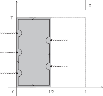
Figure 2: The world-sheet boundaries are $x=0,1/2$. The $y=0$ and $y=T$ lines are identified.

As before, we can put all the branch cuts outside the annulus. Since the integration measure is obviously the same for the two boundaries, we can again deform the contour and show that the amplitude vanishes.

3.3 Higher Loops

Generalization to higher loop is straightforward. Ref. [26] gives some details of higher loop propagator in the presence of noncommutativity. We refer the reader to [26] for our notation. The propagator in the NCOS limit is

$$\langle X^{+}(z,\bar{z})X^{-}(c=\bar{c})\rangle=4\alpha^{\prime}_{e}\left[\ln(E(z,c|iT))+\pi(T^{-1})^{ij}\Omega_{i}\Omega_{j}\right],$$ (24)

where $E(z,c)$ is the prime form, $\Omega_{i}(z,c)=\int_{c}^{z}\omega_{i}$ and $\omega_{i}$ is an Abelian differential. In the one-loop case, the prime form reduces to the theta function and the abelian differential to $dz$, hence we are back to the annulus answer (up to an irrelevant linear term).

One may wonder whether the integration measure for the massless vertex operator is the same for all boundaries thereby allowing deformation of the contour. The behavior of the prime form under coordinate transformation and modular transformation dictates that the integration measure is simply proportional to $dz$ restricted to boundary. In particular, the integration measure does not depend on the moduli parameters. As such, all the boundaries are on the same footing and the integration measure should thus be the same.

References

• [1] N. Seiberg, L. Susskind and N. Toumbas, “Strings in Background Electric Field, Space/Time Noncommutativity and A New Noncritical String Theory,” JHEP 0006 (2000) 021, hep-th/0005040;
• [2] R. Gopakumar, J.M. Maldacena, S. Minwalla and A. Strominger, “S-Duality and Noncommutative Gauge Theory,” JHEP 0006 (2000) 036, hep-th/0005048;
• [3] O.J. Ganor, G. Rajesh and S. Sethi, “Duality and Non-Commutative Gauge Theory,” Phys. Rev. D62 (2000) 125008 hep-th/0005046.
• [4] R. Gopakumar, S. Minwalla, N. Seiberg and A. Strominger, “OM Theory in Diverse Dimensions,” JHEP 0008 (2000) 008, hep-th/0006062.
• [5] I. R. Klebanov and J. Maldacena, “1+1 Dimensional NCOS and its U(N) Gauge Theory Dual”, Int. J. Mod. Phys. A16 (2001) 922; Adv. Theor. Math. Phys. 4 (2000) 283, hep-th/0006085.
• [6] G.-H. Chen and Y.-S. Wu, “Comments on Noncommutative Open String Theory: V-duality and Holography,” Phys. Rev. D63 (2001) 086003, hep-th/0006013.
• [7] J. G. Russo and M. M. Sheikh-Jabbari, “On Noncommutative Open String Theories,” JHEP 0007 (2000) 052, hep-th/0006202.
• [8] T. Kawano and S. Terashima, “S-Duality from OM-Theory,” Phys. Lett. B495 (2000) 207, hep-th/0006225.
• [9] S.-J. Rey and R. von Unge, “S-Duality, Noncritical Open String and Noncommutative Gauge Theory,” Phys. Lett. B499 (2001) 215, hep-th/0007089.
• [10] S. Hyun, “U-duality Between NCOS Theory and Matrix Theory,” Nucl. Phys. B598 (2001) 276, hep-th/0008213.
• [11] C. P. Herzog and I. R. Klebanov, “Stable Massive States in 1+1 Dimensional NCOS,” Phys. Rev. D63 (2001) 046001, hep-th/0009017.
• [12] M. Gremm, “Compactified NCOS and duality,” JHEP 0108 (2001) 052, hep-th/0009095.
• [13] J. G. Russo and M. M. Sheikh-Jabbari, “Strong Coupling Effects in non-commutative spaces from OM Theory and supergravity,” Nucl. Phys. B600 (2001) 62, hep-th/0009141.
• [14] J. Gomis and H. Ooguri, “Non-Relativistic Closed String Theory,” J. Math. Phys. 42 (2001) 3127, hep-th/0009181.
• [15] H. Larsson and P. Sundell, “Open String/Open D-Brane Dualities: Old and New,” JHEP 0106 (2001) 008, hep-th/0103188.
• [16] U. Gran and M. Nielsen, “Non-Commutative Open (p,q)-String Theories,” JHEP 0111 (2001) 022, hep-th/0104168.
• [17] C. S. Chan, A. Hashimoto and H. Verlinde, “Duality Cascade and Oblique Phases in Non-Commutative Open String Theory,” JHEP 0109 (2001) 034, hep-th/0107215.
• [18] S. Hyun and H. Shin, “ Dynamical Aspects on Duality between SYM and NCOS from D2-F1 Bound State,” hep-th/0202191.
• [19] O. Andreev and H. Dorn, “Diagrams of Noncommutative $\Phi^{3}$ Theory from String Theory,” Nucl. Phys. B583 (2000) 145, hep-th/0003113.
• [20] Y. Kiem and S. Lee, “UV/IR Mixing in Noncommutative Field Theory via Open String Loops,” Nucl. Phys. B586 (2000) 303, hep-th/0003145.
• [21] A. Bilal, C.-S. Chu and R. Russo, “String Theory and Noncommutative Field Theories at One Loop,” Nucl. Phys. B582 (2000) 65, hep-th/0003180.
• [22] J. Gomis, M. Kleban, T. Mehen, M. Rangamani and S. Shenker, “Noncommutative Gauge Dynamics From The String Worldsheet,” JHEP 0008 (2000) 011, hep-th/0003215.
• [23] A. Rajaraman and M. Rozali, “Noncommutative Gauge Theory, Divergences and Closed Strings,” JHEP 0004 (2000) 033, hep-th/0003227.
• [24] H. Liu and J. Michelson, “Stretched Strings in Noncommutative Field Theory,” Phys. Rev. D62 (2000) 066003, hep-th/0004013.
• [25] S. Chaudhuri and E. G. Novak, “Effective String Tension and Renormalizability: String Theory in a Noncommutative Space,”JHEP 0008 (2000) 027, hep-th/0006014.
• [26] Y. Kiem, S. Lee and J. Park, “Noncommutative Field Theory from String Theory: Two-loop Analysis,” Nucl. Phys. B594 (2001) 169, hep-th/0008002.