Short Distance vs. Long Distance Physics:
The Classical Limit of the Minimal Length Uncertainty Relation

Abstract

We continue our investigation of the phenomenological implications of the “deformed” commutation relations $[\hat{x}_{i},\hat{p}_{j}]=i\hbar[(1+\beta\hat{p}^{2})\delta_{ij}+\beta^{\prime}\hat{p}_{i}\hat{p}_{j}]$. These commutation relations are motivated by the fact that they lead to the minimal length uncertainty relation which appears in perturbative string theory. In this paper, we consider the effects of the deformation on the classical orbits of particles in a central force potential. Comparison with observation places severe constraints on the value of the minimum length.

I Introduction

As is well known, in the case of point particles, short distance physics directly translates into high energy physics. This is a simple consequence of the Heisenberg uncertainty principle. In local quantum field theories, which describe the dynamics of point particles, the fundamental degrees of freedom are revealed at high energy, or equivalently, at short distance. Also, there is a clear separation between ultraviolet and infrared physics from the point of view of the renormalization group.

In string theory, however, there is growing evidence that the physics at short distances, in contrast to local quantum field theory, is not clearly separated from the physics at long distances gross ; mende ; holo ; adscft ; ncft ; dscft ; dsrg . The fundamental formulation of this so–called UV/IR mixing, as well as its observable consequences, are not understood at present. Various authors have argued that some kind of UV/IR mixing is necessary to understand the cosmological constant problem banks ; cosmoc or the observable implications of short distance physics on inflationary cosmology greene .

Motivated by these questions, we have recently CMOT1 ; CMOT2 investigated various observable consequences of the UV/IR mixing embodied in the “deformed” commutation relation Kempf:1995su

$$[\hat{x},\hat{p}]=i\hbar(1+\beta\hat{p}^{2})\;.$$ (1)

This commutation relation implements the minimal length uncertainty relation

$$\Delta x\geq\frac{\hbar}{2}\left(\frac{1}{\Delta p}+\beta\,\Delta p\right)\;,$$ (2)

which appears in perturbative string theory gross ; mende . Note the UV/IR mixing manifest in Eq. (2): when the uncertainty in momentum $\Delta p$ is large (UV), the uncertainty in the position $\Delta x$ is proportional to $\Delta p$ and is therefore also large (IR). Note also that Eq. (2) implies a lower bound for $\Delta x$:

$$\Delta x\geq\hbar\sqrt{\beta}\;.$$ (3)

In the context of perturbative string theory, the existence of this minimal length is tied to the fact that strings cannot probe distances shorter than the string length scale $\ell_{S}$ . Thus,

$$\hbar\sqrt{\beta}\sim\ell_{S}\;.$$ (4)

In Ref. CMOT1 , we determined the eigenvalues and eigenfunctions of the harmonic oscillator when the position and momentum obey Eq. (1), and studied the possible constraint that can be placed on $\beta$ by precision measurements on electrons trapped in strong magnetic fields. Subsequently, in Ref. CMOT2 , we pointed out that Eq. (1) implies the finiteness of the cosmological constant and a modification of the blackbody radiation spectrum of the cosmic microwave background. One important observation made in Refs. CMOT1 ; CMOT2 was that various observable effects of the minimal length uncertainty relation are non–perturbative in the “deformation parameter” $\beta$ (i.e. contain all orders in $\beta$) even though $\beta$ appears only to linear order in Eqs. (1) and (2).

In this paper, we continue our investigation and consider the effects of the “deformation” of the canonical commutation relations on the orbits of classical particles in a central force potential. We find that comparison with observation places a strong constraint on the size of the minimum length.

II The Classical Limit

In $D$-dimensions, Eq. (1) is extended to the tensorial form Kempf:1995su :

$$[\hat{x}_{i},\hat{p}_{j}]=i\hbar(\delta_{ij}+\beta\hat{p}^{2}\delta_{ij}+\beta^{\prime}\hat{p}_{i}\hat{p}_{j})\;.$$ (5)

If the components of the momentum $\hat{p}_{i}$ are assumed to commute with each other,

$$[\hat{p}_{i},\hat{p}_{j}]=0\;,$$ (6)

then the commutation relations among the coordinates $\hat{x}_{i}$ are almost uniquely determined by the Jacobi Identity (up to possible extensions) as

$$[\hat{x}_{i},\hat{x}_{j}]=i\hbar\,\frac{(2\beta-\beta^{\prime})+(2\beta+\beta^{\prime})\beta\hat{p}^{2}}{(1+\beta\hat{p}^{2})}\left(\hat{p}_{i}\hat{x}_{j}-\hat{p}_{j}\hat{x}_{i}\right)\;.$$ (7)

In the classical limit, the quantum mechanical commutator is replaced by the Poisson bracket via

$$\frac{1}{i\hbar}[\hat{A},\hat{B}]\Longrightarrow\{A,B\}\;.$$ (8)

So the classical limits of Eqs. (5)–(7) read

$$\{x_{i},p_{j}\} = (1+\beta p^{2})\,\delta_{ij}+\beta^{\prime}p_{i}p_{j}\;,$$ (9)

$$\{p_{i},p_{j}\} = 0\;,$$ (10)

$$\{x_{i},x_{j}\} = \frac{(2\beta-\beta^{\prime})+(2\beta+\beta^{\prime})\beta p^{2}}{(1+\beta p^{2})}\left(p_{i}x_{j}-p_{j}x_{i}\right)\;.$$ (11)

We are keeping the parameters $\beta$ and $\beta^{\prime}$ fixed as $\hbar\rightarrow 0$, which in the string theory context corresponds to keeping the string momentum scale fixed while the string length scale is taken to zero.

Note that for Eq. (8) to make sense, the Poisson bracket must possess the same properties as the quantum mechanical commutator, namely, it must be anti-symmetric, bilinear, and satisfy the Leibniz rules and the Jacobi Identity. These requirements allows us to derive the general form of our Poisson bracket for any functions of the coordinates and momenta as

$$\{F,G\}=\left(\frac{\partial F}{\partial x_{i}}\frac{\partial G}{\partial p_{j}}-\frac{\partial F}{\partial p_{i}}\frac{\partial G}{\partial x_{j}}\right)\{x_{i},p_{j}\}+\frac{\partial F}{\partial x_{i}}\frac{\partial G}{\partial x_{j}}\{x_{i},x_{j}\}\;,$$ (12)

where repeated indices are summed. In particular, we find that the time evolutions of the coordinates and momenta are governed by

$$\dot{x}_{i} = \{x_{i},H\}\;=\;\phantom{-}\{x_{i},p_{j}\}\,\frac{\partial H}{\partial p_{j}}+\{x_{i},x_{j}\}\,\frac{\partial H}{\partial x_{j}}\;,$$ (13)

$$\dot{p}_{i} = \{p_{i},H\}\;=\;-\{x_{i},p_{j}\}\,\frac{\partial H}{\partial x_{j}}\;.$$ (14)

This “deformed” version of classical mechanics is not without its difficulties, the foremost being how one can construct “canonical transformations” which relate the dynamical variables at one length scale to those at another. For the minimal length to be a well defined length scale, all dynamical variables at all length scales must obey Eq. (11). As a consequence, for instance, one cannot identify the position of a composite particle with the center of mass of its constituents. In retrospect, it is not surprising that this difficulty would exist given the UV/IR mixing nature of Eqs. (5)–(7) from which Eqs. (11) have been derived.

We merely point out this difficulty as a caveat and do not attempt to propose any solution in the current paper. Instead, we apply Eq. (14) to the motion of macroscopic objects and look for signatures of the deformation.

III Motion in Central Force Potentials

For the Hamiltonian of a particle in a central force potential,

$$H=\frac{p^{2}}{2m}+V(r)\;,\qquad r=\sqrt{x_{i}x_{i}}\;,$$ (15)

the derivatives with respect to the coordinates and momenta are

$$\frac{\partial H}{\partial p_{j}}=\frac{p_{j}}{m}\;,\qquad\frac{\partial H}{\partial x_{j}}=\frac{\partial V}{\partial r}\frac{x_{j}}{r}\;.$$ (16)

Therefore, the time evolutions of the coordinates and momenta in this case are

$$\dot{x}_{i} = [\,1+(\beta+\beta^{\prime})p^{2}\,]\,\frac{p_{i}}{m}-[\,(2\beta-\beta^{\prime})+(2\beta+\beta^{\prime})\beta p^{2}\,]\left(\frac{1}{r}\frac{\partial V}{\partial r}\right)L_{ij}\,x_{j}\;,$$ (17)

$$\dot{p}_{i} = -[\,(1+\beta p^{2})\,x_{i}+\beta^{\prime}(p\cdot x)\,p_{i}\,]\left(\frac{1}{r}\frac{\partial V}{\partial r}\right)\;,$$ (18)

where

$$L_{ij}\equiv\frac{x_{i}p_{j}-x_{j}p_{i}}{(1+\beta p^{2})}\;.$$

The $L_{ij}$’s defined here are the generators of rotation:

$$\{x_{k},L_{ij}\}=x_{i}\,\delta_{kj}-x_{j}\,\delta_{ki}\;,\qquad\{p_{k},L_{ij}\}=p_{i}\,\delta_{kj}-p_{j}\,\delta_{ki}\;.$$ (19)

For motion in a central force potential, the $L_{ij}$’s are conserved due to rotational symmetry:

$$\{L_{ij},H\}=0\;.$$ (20)

So is

$$L^{2}\equiv-\frac{1}{2}L_{ij}L_{ji}=\frac{p^{2}\,r^{2}-(p\cdot x)^{2}}{(1+\beta p^{2})^{2}}\;.$$ (21)

The conservation of the $L_{ij}$’s imply that the motion of the particle will be confined to a 2-dimensional plane spanned by the coordinate and momentum vectors at any point in time. Therefore, without loss of generality, we can assume that the motion is in the $x_{1}x_{2}$-plane and

$$L_{12}=-L_{21}=L\;,\qquad L_{ij}=0\quad\mbox{otherwise}\;.$$ (22)

Then, the motion can be described by the time dependences of the distance from the origin $r$, and the angle

$$\phi\equiv\tan^{-1}\frac{x_{2}}{x_{1}}\;.$$ (23)

The equation of motion for $r$ is given by

$$\dot{r} = \frac{1}{2r}\frac{d}{dt}(r^{2})\;=\;\frac{1}{2r}\frac{d}{dt}(x_{i}x_{i})\;=\;\frac{x_{i}}{r}\,\dot{x_{i}}$$ (24)

$$= \frac{1}{m}[\,1+(\beta+\beta^{\prime})p^{2}\,]\,p_{r}\;,$$ (25)

where

$$p_{r}\equiv\frac{(p\cdot x)}{r}=\sqrt{p^{2}-\frac{L^{2}(1+\beta p^{2})^{2}}{r^{2}}}\;.$$ (26)

Since the energy, $E$, is also conserved, we can write the momentum squared as a function of $r$ via

$$p^{2}=2m[\,E-V(r)\,]\;.$$ (27)

Therefore, right hand side of Eq. (25) can be written completely in terms of conserved quantities and functions of $r$:

$$\frac{dr}{dt}=\frac{1}{m}\biggl{[}1+2m(\beta+\beta^{\prime})(E-V)\biggr{]}\sqrt{2m(E-V)-\frac{\displaystyle L^{2}\left[1+2m\beta(E-V)\right]^{2}}{\displaystyle r^{2}}}\;.$$ (28)

The equation of motion for the angle $\phi$ is

$$\dot{\phi} = \frac{x_{1}\dot{x_{2}}-x_{2}\dot{x_{1}}}{r^{2}}$$ (29)

$$= \frac{L}{mr^{2}}\left\{[\,1+(\beta+\beta^{\prime})p^{2}\,](1+\beta p^{2})+[\,(2\beta-\beta^{\prime})+(2\beta+\beta^{\prime})\beta p^{2}\,]\left(mr\frac{\partial V}{\partial r}\right)\right\}\;.$$ (30)

Again, using Eq. (27), the right hand side can be written in terms of conserved quantities and functions of $r$ only:

$$\frac{d\phi}{dt} = \frac{L}{mr^{2}}\Biggl{\{}\left[\,1+2m(\beta+\beta^{\prime})(E-V)\,\right]\left[\,1+2m\beta(E-V)\,\right]\Biggr{.}$$ (32)

$$\Biggl{.}+\left[\,(2\beta-\beta^{\prime})+2m\beta(2\beta+\beta^{\prime})(E-V)\,\right]\left(\,mr\frac{\partial V}{\partial r}\,\right)\Biggr{\}}\;.$$

From Eqs. (28) and (32), we find

$$\frac{d\phi}{dr}=\frac{L}{r^{2}}\,\frac{\displaystyle 1+2m\beta(E-V)+\frac{\displaystyle(2\beta-\beta^{\prime})+2m\beta(2\beta+\beta^{\prime})(E-V)}{\displaystyle 1+2m(\beta+\beta^{\prime})(E-V)}\left(mr\frac{\partial V}{\partial r}\right)}{\displaystyle\sqrt{2m(E-V)-\frac{\displaystyle L^{2}\left[1+2m\beta(E-V)\right]^{2}}{\displaystyle r^{2}}}}\;.$$ (33)

In principle, this equation can be integrated to obtain the $\phi$ dependence of $r$. We will solve Eq. (33) for the harmonic oscillator and Coulomb potentials in the following two cases:

1. $\beta\neq 0$, $\beta^{\prime}=0$, in which Eq. (33) simplifies to

   $$\frac{d\phi}{dr}=\frac{L}{r^{2}}\,\frac{\displaystyle 1+2m\beta\left(E-V+r\frac{\partial V}{\partial r}\right)}{\displaystyle\sqrt{2m(E-V)-\frac{\displaystyle L^{2}\left[1+2m\beta(E-V)\right]^{2}}{\displaystyle r^{2}}}}\;,$$ (34)

   and

2. $\beta=0$, $\beta^{\prime}\neq 0$, in which Eq. (33) simplifies to

   $$\frac{d\phi}{dr}=\frac{L}{r^{2}}\,\frac{\displaystyle\;\;1-\frac{\displaystyle 1}{\displaystyle(1/\beta^{\prime})+2m(E-V)}\left(mr\frac{\partial V}{\partial r}\right)\;\;}{\displaystyle\sqrt{2m(E-V)-\frac{\displaystyle L^{2}}{\displaystyle r^{2}}}}\;.$$ (35)

IV The Harmonic Oscillator Potential

We first consider the harmonic oscillator potential

$$V(r)=\frac{1}{2}m\omega^{2}r^{2}\;.$$ (36)

IV.1 $\beta\neq 0$, $\beta^{\prime}=0$ case

For the harmonic oscillator, Eq. (34) can be cast into the form

$$\frac{d\phi}{dr^{2}}=\frac{1}{2}\left[\frac{r_{\max}r_{\min}}{r^{2}\sqrt{(r_{\max}^{2}-r^{2})(r^{2}-r_{\min}^{2})}}+\frac{\sin\alpha}{\sqrt{(r_{\max}^{2}-r^{2})(r^{2}-r_{\min}^{2})}}\right]\;,$$ (37)

where

$$r^{2}_{\max/\min} \equiv \frac{E+\beta m\omega^{2}L^{2}(1+2m\beta E)\pm\sqrt{E^{2}-\omega^{2}L^{2}(1+2m\beta E)}}{m\omega^{2}(1+\beta^{2}m^{2}\omega^{2}L^{2})}$$ (38)

$$= r_{\pm}^{2}\mp\left(\frac{2\,r_{\pm}\,r_{\mp}^{3}}{r_{+}^{2}-r_{-}^{2}}\right)\varepsilon\mp\left\{\frac{r_{\mp}^{4}(5r_{\pm}^{4}-2r_{+}^{2}r_{-}^{2}+r_{\mp}^{4})}{(r_{+}^{2}-r_{-}^{2})^{3}}\right\}\varepsilon^{2}+\mathcal{O}(\varepsilon^{3})\;,$$ (39)

and

$$r_{\pm}^{2} \equiv \left(\frac{E\pm\sqrt{E^{2}-\omega^{2}L^{2}}}{m\omega^{2}}\right)\;,$$ (40)

$$\varepsilon \equiv \tan\alpha\;\equiv\;\beta m\omega L\;.$$ (41)

$r_{\max/\min}$ are the turning points when $\beta\neq 0$ and $r_{\pm}$ are the turning points when $\beta=0$. When $\varepsilon=\beta m\omega L$ satisfies the condition

$$0<\varepsilon<\frac{(r_{+}^{2}-r_{-}^{2})^{2}}{4r_{+}r_{-}(r_{+}^{2}+r_{-}^{2})}\;,$$ (42)

it is possible to show that

$$r_{-}<r_{\min}<r_{\max}<r_{+}\;.$$ (43)

When $\varepsilon=\beta m\omega L$ exceeds the upper bound of the region Eq. (42), no solution exists.

Eq. (37) can be integrated to yield

$$\phi(r) = \frac{1}{2}\left[\arcsin\left\{\frac{(r^{2}-r^{2}_{\min})\,r^{2}_{\max}-(r^{2}_{\max}-r^{2})\,r^{2}_{\min}}{(r^{2}_{\max}-r^{2}_{\min})\,r^{2}}\right\}\right.$$ (45)

$$\left.\quad+\sin\alpha\,\arcsin\left\{\frac{(r^{2}-r^{2}_{\min})-(r^{2}_{\max}-r^{2})}{(r^{2}_{\max}-r^{2}_{\min})}\right\}\right]\;.$$

In particular, we find

$$\phi(r_{\max})-\phi(r_{\min})=\frac{\pi}{2}\left(1+\sin\alpha\right)\;,$$ (46)

which shows that the orbit will not close on itself when $\beta\neq 0$. It precesses by an angle of $2\pi\sin\alpha$ per revolution. For $\beta\ll 1$, the precession angle is

$$\Delta\omega_{\beta}=2\pi\sin\alpha\approx 2\pi(\,\beta m\omega L\,)\;.$$ (47)

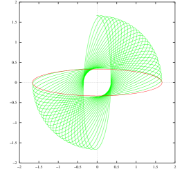
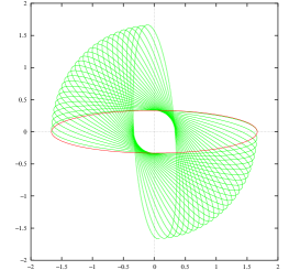
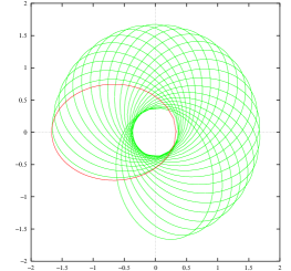
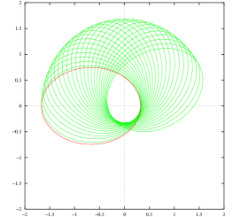
Figure 1: The trajectory of a mass in a harmonic oscillator potential with $r_{+}/r_{-}=5$, $\beta m\omega L=0.01$, $\beta^{\prime}=0$ (left), and $\beta=0$, $\beta^{\prime}m\omega L=0.01$ (right). The length scale is in units of $(r_{+}+r_{-})/2$. The red line indicates the orbit when $\beta=\beta^{\prime}=0$. The motion is counter clockwise along the trajectory starting from the aphelion on the positive $x$ axis. 25 complete revolutions are shown. The trajectory is precessing counter clockwise on the left, and clockwise on the right.

Figure 2: The trajectory of a mass in a coulomb potential with $r_{+}/r_{-}=5$, $2m|E|\beta=0.01$, $\beta^{\prime}=0$ (left), and $\beta=0$, $2m|E|\beta^{\prime}=0.01$ (right). The length scale is in units of $(r_{+}+r_{-})/2$. The red line indicates the orbit when $\beta=\beta^{\prime}=0$. The motion is counter clockwise along the trajectory starting from the perihelion on the positive $x$ axis. 25 complete revolutions are shown. For both cases, the trajectory is precessing clockwise.

In Figure (2), we plot the trajectory of the motion for a representative set of parameters.

IV.2 $\beta=0$, $\beta^{\prime}\neq 0$ case

For the harmonic oscillator, Eq. (35) can be cast into the form

$$\frac{d\phi}{dr^{2}}=\frac{r_{+}r_{-}}{2}\left(\frac{1}{r^{2}}-\frac{1}{r_{\beta^{\prime}}^{2}-r^{2}}\right)\frac{1}{\sqrt{(r_{+}^{2}-r^{2})(r^{2}-r_{-}^{2})}}$$ (48)

where

$$r_{\pm}^{2} \equiv \left(\frac{E\pm\sqrt{E^{2}-\omega^{2}L^{2}}}{m\omega^{2}}\right)\;,$$ (49)

$$r_{\beta^{\prime}}^{2} \equiv r_{+}^{2}+r_{-}^{2}+\frac{1}{m^{2}\omega^{2}\beta^{\prime}}\;.$$ (50)

Note that the turning points, $r_{\pm}$, do not depend on $\beta^{\prime}$. In the limit $\beta^{\prime}\rightarrow 0$, we have $r_{\beta^{\prime}}^{2}\rightarrow\infty$, and the equation for the $\beta=\beta^{\prime}=0$ case is recovered.

Eq. (48) can be integrated to yield

$$\phi(r^{2}) = \frac{1}{2}\left[\arcsin\left\{\frac{(r^{2}-r_{-}^{2})\,r_{+}^{2}-(r_{+}^{2}-r^{2})\,r_{-}^{2}}{(r_{+}^{2}-r_{-}^{2})\,r^{2}}\right\}\right.$$ (52)

$$\quad-\sin\alpha_{+}\sin\alpha_{-}\left.\arcsin\left\{\frac{(r_{\beta^{\prime}}^{2}-r_{+}^{2})(r^{2}-r_{-}^{2})-(r_{\beta^{\prime}}^{2}-r_{-}^{2})(r_{+}^{2}-r^{2})}{(r_{\beta^{\prime}}^{2}-r^{2})(r_{+}^{2}-r_{-}^{2})}\right\}\right]\;,$$

where

$$\tan\alpha_{\pm}\equiv r_{\pm}m\omega\sqrt{\beta^{\prime}}\;.$$ (53)

Note that $\alpha_{\pm}\rightarrow 0$ in the limit $\beta^{\prime}\rightarrow 0$. From Eq. (52), we find

$$\phi(r_{+})-\phi(r_{-})=\frac{\pi}{2}\left(1-\sin\alpha_{+}\sin\alpha_{-}\right)\;.$$ (54)

Compared to the $\beta\neq 0$, $\beta^{\prime}=0$ case, Eq. (46), the precession is in the opposite direction: for each revolution, the angle swept is smaller than $2\pi$ by $2\pi\sin\alpha_{+}\sin\alpha_{-}$. For $\beta^{\prime}\ll 1$, the precession angle is

$$\Delta\omega_{\beta^{\prime}}=-2\pi\,\sin\alpha_{+}\sin\alpha_{-}\approx-2\pi(\,\beta^{\prime}m\omega L\,)\;.$$ (55)

In Figure (2), we plot the trajectory of the motion for a representative set of parameters.

V The Coulomb Potential

Next, we consider the attractive Coulomb potential

$$V(r)=-\frac{k}{r}\;,\qquad(k>0)\;.$$ (56)

V.1 $\beta\neq 0$, $\beta^{\prime}=0$ case

For bound states, $E=-|E|$, Eq. (34) takes on the form

$$\frac{d\phi}{dr}=\sqrt{r_{+}r_{-}}\frac{\displaystyle 1-\varepsilon\left\{1-\frac{2(r_{+}+r_{-})}{r}\right\}}{\displaystyle\sqrt{(r-\delta)(r-\delta^{*})(r_{\max}-r)(r-r_{\min})}}\;,$$ (57)

where

$$\varepsilon \equiv 2m|E|\beta\;,$$ (58)

$$r_{\pm} \equiv \frac{k}{2|E|}\pm\sqrt{\frac{k^{2}}{4E^{2}}-\frac{L^{2}}{2m|E|}}\;,$$ (59)

and

$$r_{\max/\min} = r_{\pm}-\left(\frac{2r_{\mp}^{2}}{r_{\pm}-r_{\mp}}\right)\varepsilon-\left\{\frac{r_{\mp}^{3}(r_{+}+r_{-})(5r_{\pm}-3r_{\mp})}{r_{\pm}(r_{\pm}-r_{\mp})^{3}}\right\}\varepsilon^{2}+\mathcal{O}(\varepsilon^{3})\;,$$ (60)

$$\delta = -\,\varepsilon\,(r_{+}+r_{-})\left[1+\left\{1-\frac{3\,(r_{+}+r_{-})^{2}}{2\,r_{+}r_{-}}\right\}\varepsilon+\mathcal{O}(\varepsilon^{2})\right]$$ (62)

$$+\,i\,\varepsilon^{3/2}\,\frac{(r_{+}+r_{-})^{2}}{\sqrt{r_{+}r_{-}}}\left[1+\frac{3}{8}\left\{1-\frac{7\,(r_{+}+r_{-})^{2}}{8\,r_{+}r_{-}}\right\}\varepsilon+\mathcal{O}(\varepsilon^{2})\right]\;.$$

The exact forms of $\delta$ and $r_{\max/\min}$ are rather lengthy and non-illuminating, so we will not present them here. (See appendix A.) $r_{\pm}$ are the turning points when $\beta=0$, and we can see that when $\beta>0$,

$$r_{-}<r_{\min}<r_{\max}<r_{+}\;,$$ (63)

just as in the harmonic oscillator case. The condition that $\varepsilon=2m|E|\beta$ must satisfy for the solution to exist is

$$\frac{r_{+}r_{-}}{(r_{+}+r_{-})^{2}}>\frac{8(1-\varepsilon)^{4}}{1-33\varepsilon-33\varepsilon^{2}+\varepsilon^{3}+(1+14\varepsilon+\varepsilon^{2})^{3/2}}\;.$$ (64)

Eq. (57) can be integrated and the solution expressed exactly in terms of elliptic integrals. (See appendix B.) However, the exact expression is not particularly informative so we present the solution to linear order in $\beta$, in which case we find

$$\phi(r) = \left[1-\frac{(r_{\max}+r_{\min})^{2}}{2\,r_{\max}r_{\min}}\,\varepsilon\right]\arcsin\left\{\frac{(r-r_{\min})r_{\max}-(r_{\max}-r)r_{\min}}{(r_{\max}-r_{\min})r}\right\}$$ (66)

$$+\frac{(r_{\max}+r_{\min})}{r}\sqrt{\frac{(r_{\max}-r)(r-r_{\min})}{r_{\max}r_{\min}}}\,\varepsilon+\mathcal{O}(\varepsilon^{2})\;,$$

and

$$\phi(r_{\max})-\phi(r_{\min})=\pi\left[1-\frac{(r_{\max}+r_{\min})^{2}}{2\,r_{\max}r_{\min}}\,\varepsilon+\mathcal{O}(\varepsilon^{2})\right]\;.$$ (67)

Note that, in contrast to the harmonic oscillator, the precession angle is negative:

$$\Delta\omega_{\beta}\approx-2\pi\left\{\frac{(r_{\max}+r_{\min})^{2}}{2\,r_{\max}r_{\min}}\,\varepsilon\right\}=-2\pi\left(\frac{4m|E|\beta}{1-e^{2}}\right)\;,$$ (68)

where $e$ is the eccentricity of the orbit. This means that the perihelion of a planet in a gravitational Coulomb potential will retard instead of advance. In Figure (2), we plot the trajectory of the motion for a representative set of parameters.

V.2 $\beta=0$, $\beta^{\prime}\neq 0$ case

For bound states, $E=-|E|$, Eq. (35) takes on the form

$$\frac{d\phi}{dr}=\frac{\sqrt{r_{+}r_{-}}}{2}\left(\frac{1}{r}+\frac{1}{r+r_{\beta^{\prime}}}\right)\frac{1}{\sqrt{(r_{+}-r)(r-r_{-})}}\;,$$ (69)

where

$$r_{\pm} \equiv \frac{k}{2|E|}\pm\sqrt{\frac{k^{2}}{4E^{2}}-\frac{L^{2}}{2m|E|}}\;,$$ (70)

$$r_{\beta^{\prime}} \equiv \frac{\displaystyle(r_{+}+r_{-})}{\displaystyle\;\;\left(\frac{\displaystyle 1}{\displaystyle 2m|E|\beta^{\prime}}\right)-1\;\;}\;.$$ (71)

As in the harmonic oscillator case, the turning points $r_{\pm}$ do not depend on $\beta^{\prime}$. In the limit $\beta^{\prime}\rightarrow 0$, we have $r_{\beta^{\prime}}\rightarrow 0$, and the equation for the $\beta=\beta^{\prime}=0$ case is recovered.

Eq. (69) can be integrated to yield,

$$\phi(r) = \frac{1}{2}\left[\arcsin\left\{\frac{(r-r_{-})\,r_{+}-(r_{+}-r)\,r_{-}}{(r_{+}-r_{-})\,r}\right\}\right.$$ (73)

$$\quad\left.+\cos\theta_{+}\cos\theta_{-}\arcsin\left\{\frac{(r_{+}+r_{\beta^{\prime}})(r-r_{-})-(r_{-}+r_{\beta^{\prime}})(r_{+}-r)}{(r+r_{\beta^{\prime}})(r_{+}-r_{-})}\right\}\right]\;,$$

where

$$\tan\theta_{\pm}=\sqrt{\frac{r_{\beta^{\prime}}}{r_{\pm}}}\;.$$ (74)

Note that $\theta_{\pm}\rightarrow 0$ in the limit $\beta^{\prime}\rightarrow 0$. From Eq. (73), we find

$$\phi(r_{+})-\phi(r_{-})=\frac{\pi}{2}\left(1+\cos\theta_{+}\cos\theta_{-}\right)=\pi\left[1-\left(\frac{1-\cos\theta_{+}\cos\theta_{-}}{2}\right)\right]\;.$$ (75)

As in the harmonic oscillator case, the precession angle is negative when $\beta^{\prime}$ is positive. For $\beta^{\prime}\ll 1$, the precession angle is

$$\Delta\omega_{\beta^{\prime}}=-2\pi\left(\frac{1-\cos\theta_{+}\cos\theta_{-}}{2}\right)\approx-2\pi\left\{\frac{(r_{+}+r_{-})^{2}}{4\,r_{+}r_{-}}(2m|E|\beta^{\prime})\right\}=-2\pi\left(\frac{2m|E|\beta^{\prime}}{1-e^{2}}\right)\;.$$ (76)

In Figure (2), we plot the trajectory of the motion for a representative set of parameters.

VI Comparison with Planetary Orbits

Using our results, we can place constraints on $\beta$ and $\beta^{\prime}$ from the precession of the perihelion of Mercury. According to Ref. Mercury , the observed advance of the perihelion of Mercury that is unexplained by Newtonian planetary perturbations or solar oblateness is

$$\Delta\omega_{\mathrm{obs}} = 42.980\pm 0.002\;\mbox{arc-seconds per century}$$ (77)

$$= \frac{2\pi\,(\,3.31636\pm 0.00015\,)\times 10^{-5}\,\mathrm{radians}}{415.2019\;\mathrm{revolutions}}$$ (78)

$$= 2\pi\,(\,7.98734\pm 0.00037\,)\times 10^{-8}\,\mathrm{radians/revolution}\;.$$ (79)

This advance is usually explained by General Relativity which predicts

$$\Delta\omega_{\mathrm{GR}}=3\pi\left\{\frac{2\,GM_{\odot}/c^{2}}{a\,(1-e^{2})}\right\}=6\pi\left\{\frac{2m|E|}{(1-e^{2})\,\hbar^{2}}\right\}\left(\frac{\hbar^{2}}{m^{2}c^{2}}\right)=6\pi\left(\frac{\lambdabar_{c}}{\lambdabar_{d}}\right)^{2}\;,$$ (80)

where $2\,GM_{\odot}/c^{2}$ is the Schwarzschild radius of the Sun, $a$ is the semi-major axis of the planet’s orbit, $e$ is it’s eccentricity, and we have defined

$$\lambdabar_{d}\equiv\hbar\sqrt{\frac{(1-e^{2})}{2m|E|}}\;,\qquad\lambdabar_{c}\equiv\frac{\hbar}{mc}\;.$$ (81)

The lengths $\lambdabar_{d}$ and $\lambdabar_{c}$ are the de Broglie and Compton wavelengths of the planet. For Mercury, the parameters are AstroData

$$\frac{2\,GM_{\odot}}{c^{2}} = 2.95325008\times 10^{3}\,\mathrm{m}\;,$$ (82)

$$m = 3.3022\times 10^{23}\,\mathrm{kg}\;,$$ (83)

$$a\;=\;\frac{r_{\max}+r_{\min}}{2} = 5.7909175\times 10^{10}\,\mathrm{m}\;,$$ (84)

$$e = 0.20563069\;.$$ (85)

Note that the product $GM_{\odot}$ is known to much better accuracy than Newton’s gravitational constant $G$ and the solar mass $M_{\odot}$ separately. Using these parameters we find

$$\lambdabar_{d} = 6.5284\times 10^{-63}\,\mathrm{m}\;,$$ (86)

$$\lambdabar_{c} = 1.0653\times 10^{-66}\,\mathrm{m}\;,$$ (87)

and

$$\Delta\omega_{\mathrm{GR}}=2\pi\,(\,7.98744\times 10^{-8}\,)\,\mathrm{radians/revolution}\;.$$ (88)

Comparison of Eqs. (88) and (79) yields

$$\Delta\omega_{\mathrm{obs}}-\Delta\omega_{\mathrm{GR}}=2\pi\,(\,-0.00010\pm 0.00037\,)\times 10^{-8}\,\mathrm{radians/revolution}\;,$$ (89)

which is consistent with zero. As we can see, there is not much room left for possible extra contributions to the precession.

From Eq. (68) and (76), the precession angle to linear order in $\beta$ and $\beta^{\prime}$ is

$$\Delta\omega_{\beta}+\Delta\omega_{\beta^{\prime}}=-2\pi\left\{\frac{\hbar^{2}(2\beta+\beta^{\prime})}{\lambdabar_{d}^{2}}\right\}\;.$$ (90)

The existence of a minimal length requires

$$\beta>0\;,\qquad\beta+\beta^{\prime}>0\;,$$ (91)

so we can assume that

$$\Delta\omega_{\beta}+\Delta\omega_{\beta^{\prime}}<-2\pi\left(\frac{\hbar\sqrt{\beta}}{\lambdabar_{d}}\right)^{2}<0\;.$$ (92)

Eq. (89) places a lower bound on $\Delta\omega_{\beta}+\Delta\omega_{\beta^{\prime}}$ which at $3\sigma$ is

$$-2\pi\,(\,1.2\times 10^{-11}\,)\,\mathrm{radians/revolution}<(\,\Delta\omega_{\beta}+\Delta\omega_{\beta^{\prime}}\,)<-2\pi\left(\frac{\hbar\sqrt{\beta}}{\lambdabar_{d}}\right)^{2}\;.$$ (93)

Thus,

$$\left(\frac{\hbar\sqrt{\beta}}{\lambdabar_{d}}\right)^{2}<1.2\times 10^{-11}\;,$$ (94)

or

$$\hbar{\sqrt{\beta}}<(3.5\times 10^{-6})\,\lambdabar_{d}=2.3\times 10^{-68}\,\mathrm{m}\;.$$ (95)

Note that this limit is 33 orders of magnitude below the Planck length!

VII Discussion and Conclusion

In this paper, we have considered the effects of the minimal length uncertainty relation on the classical orbits of particles in a central force potential. Comparison with the observed precession of the perihelion of Mercury places a strong constraint on the value of the minimum length.

The minimal length uncertainty relation was implemented through the deformed commutation relation Eq. (5). Note that even though $\beta$ and $\beta^{\prime}$ appear to only linear order on the right hand side of Eq. (5), our expressions for the precession angle, Eqs. (46), (54), (67), and (75), contain all orders in $\beta$ and $\beta^{\prime}$. In that sense, our results are non-perturbative. On the other hand, the right hand side of Eq. (5) itself can be considered a linear approximation to a more general expression which leads to the minimal length uncertainty relation as discussed by Kempf Kempf:1995su . This suggests that our constraint, Eq. (95), could be fairly robust. All other possible implementation of the minimal length uncertainty relation can be expected to lead to the same precession of the perihelion as Eq. (5) to linear order in $\beta$ and $\beta^{\prime}$, and result in the same constraint on the minimal length.

The analysis of this paper based on the deformed commutation relations can be viewed as providing a toy model for a full string theoretic consideration of the implications of the minimal length uncertainty relation. The natural question to ask is whether our constraint, Eq. (95), applies to string theory proper or not. This is a difficult question to answer since the minimal length uncertainty relation is but one aspect of string theory, and it is not clear whether deforming the quantum mechanical commutation relations is the correct way to implement it.

Looking at previous works, we note that Ref. mende has discussed departures from General Relativity as implied by string theory. These were implied both by the string theoretic modification of Einstein’s equations GSW

$$R_{\mu\nu}+\frac{\alpha^{\prime}}{2}R_{\mu\kappa\lambda\tau}R_{\nu}^{\kappa\lambda\tau}+\cdots=0\;,$$ (96)

as well as the crucial distinctions between particles and strings: strings as extended objects do not fall freely along geodesics. As fundamentally extended objects (at least from the point of view of string perturbation theory) they are subject to tidal forces. This leads, for example, to an energy dependent deflection angle for the bending of light – in clear distinction to General Relativity in which the deflection angle is energy independent. We have not included in our analysis any of these effects. In particular, we have not considered possible deviations in the background metric due to the extra terms in Eq. (96). Though the corrections to particle trajectories due to such deviations are expected to be small, it may be worthwhile to study the problem in more detail in light of the strong constraint we have obtained for the minimal length.

We conclude by listing a few more caveats: Even though our analysis is purely classical, the general formulation of classical systems which incorporates the classical limit of the minimal length uncertainty relation is not fully understood. How one can define the “canonical transformations” which relate dynamical variables at different scales while preserving the Poisson bracket remains an open problem. Also, the systems we considered have only a finite number of degrees of freedom. It is not clear how to incorporate the effects of the classical limit of the minimal length uncertainty relation to field theory. The classical limit of the minimal length uncertainty relation provides a natural generalization of the non–commutative relation between spatial coordinates encountered in non–commutative field theory ncft . What is not clear is whether the usual Weyl–Wigner–Moyal technology moyal could apply even in our more complicated set-up, thus providing a way to analyze systems with an infinite number of degrees of freedom.

Appendix A The Turning Points for the Coulomb Potential

The turning points for the Coulomb Potential, Eq. (56), are provided by the real solutions to

$$2m\left(-|E|+\frac{k}{r}\right)-\frac{L^{2}}{r^{2}}\left[1+2m\beta\left(-|E|+\frac{k}{r}\right)\right]^{2}=0\;.$$ (97)

Defining

$$A\equiv\frac{k}{|E|}\;,\qquad B\equiv\frac{L^{2}}{2m|E|}\;,\qquad\varepsilon\equiv 2m|E|\beta\;,$$ (98)

Eq. (97) can be cast into the form

$$r^{4}-A\,r^{3}+B(1-\varepsilon)^{2}r^{2}+2AB\varepsilon(1-\varepsilon)\,r+A^{2}B\varepsilon^{2}=0\;.$$ (99)

Since this is a quartic equation, the solutions can be obtained algebraically (using Mathematica) and they are:

$$\delta\phantom{{}^{*}} = \frac{1}{4}(A-W+2iX)\;,$$ (100)

$$\delta^{*} = \frac{1}{4}(A-W-2iX)\;,$$ (101)

$$r_{\max} = \frac{1}{4}(A+W+2Y)\;,$$ (102)

$$r_{\min} = \frac{1}{4}(A+W-2Y)\;,$$ (103)

where

$$W \equiv \frac{1}{\sqrt{3}}\sqrt{3A^{2}-8B(1-\varepsilon)^{2}+4Z+\frac{4B\left\{B(1-\varepsilon)^{4}+6A^{2}\varepsilon(1+\varepsilon)\right\}}{Z}}$$ (104)

$$= A+4A\,\varepsilon+\left(4A-\frac{6A^{3}}{B}\right)\varepsilon^{2}+\cdots\;,$$ (105)

$$X \equiv \frac{1}{2}\sqrt{-3A^{2}+8B(1-\varepsilon)^{2}+W^{2}+\frac{2A\left\{A^{2}-4B(1-\varepsilon)(1+3\varepsilon)\right\}}{W}}$$ (106)

$$= \frac{2A^{2}}{\sqrt{B}}\,\varepsilon^{3/2}+\frac{3A^{2}(8B-7A^{2})}{4\sqrt{B^{3}}}\,\varepsilon^{5/2}+\cdots\;,$$ (107)

$$Y \equiv \frac{1}{2}\sqrt{3A^{2}-8B(1-\varepsilon)^{2}-W^{2}+\frac{2A\left\{A^{2}-4B(1-\varepsilon)(1+3\varepsilon)\right\}}{W}}$$ (108)

$$= \sqrt{A^{2}-4B}-\frac{2(A^{2}-2B)}{\sqrt{A^{2}-4B}}\,\varepsilon+\frac{A^{2}(3A^{4}-20A^{2}B+30B^{2})}{B\sqrt{(A^{2}-4B)^{3}}}\,\varepsilon^{2}+\cdots\;,$$ (109)

$$Z \equiv \Biggl{[}\frac{1}{2}\Biggl{\{}2B^{3}(1-\varepsilon)^{6}+18A^{2}B^{2}\varepsilon(1+\varepsilon)(1-\varepsilon)^{2}+27A^{4}B\varepsilon^{2}\Biggr{.}\Biggr{.}$$ (111)

$$\Biggl{.}\Biggl{.}+3\sqrt{3}A^{2}B\varepsilon^{3/2}\sqrt{27A^{4}\varepsilon+4A^{2}B(1+\varepsilon)(1-34\varepsilon+\varepsilon^{2})-16B^{2}(1-\varepsilon)^{4}}\Biggr{\}}\Biggr{]}^{1/3}$$

$$= B+(3A^{2}-2B)\,\varepsilon+\frac{A^{2}\sqrt{3B(A^{2}-4B)}}{B}\,\varepsilon^{3/2}+\left(9A^{2}+B-\frac{9A^{4}}{2B}\right)\varepsilon^{2}+\cdots\;.$$ (112)

In the limit $\varepsilon\rightarrow 0$, we recover the turning points for the $\beta=0$ case:

$$\delta,\delta^{*}\rightarrow 0\;,\qquad r_{\max/\min}\rightarrow r_{\pm}=\frac{A\pm\sqrt{A^{2}-4B}}{2}\;.$$ (113)

Appendix B The Solution to the Coulomb Problem in terms of Elliptic Integrals

Integration of Eq. (57) yields

$$\phi(r)=\sqrt{r_{+}r_{-}}\,(1-\varepsilon)\,I_{0}+2\sqrt{r_{+}r_{-}}\,(r_{+}+r_{-})\,\varepsilon\,I_{1}\;,$$ (114)

where

$$I_{0} = \int\frac{dr}{\sqrt{(r-\delta)(r-\delta^{*})(r_{\mathrm{max}}-r)(r-r_{\mathrm{min}})}}\;,$$ (115)

$$I_{1} = \int\frac{dr}{r\sqrt{(r-\delta)(r-\delta^{*})(r_{\mathrm{max}}-r)(r-r_{\mathrm{min}})}}\;.$$ (116)

These integrals can be expressed in terms of the Legendre–Jacobi elliptic integrals groebner :

$$F(\psi,k^{2}) = \int_{0}^{\psi}\frac{d\eta}{\sqrt{1-k^{2}\sin^{2}\eta}}\;,$$ (117)

$$\Pi(\psi,\rho,k^{2}) = \int_{0}^{\psi}\frac{d\eta}{(1+\rho\sin^{2}\eta)\sqrt{1-k^{2}\sin^{2}\eta}}\;.$$ (118)

Define

$$\cos\psi\equiv\frac{U_{\!-}(r_{\mathrm{max}}-r)-U_{\!+}(r-r_{\mathrm{min}})}{U_{\!-}(r_{\mathrm{max}}-r)+U_{\!+}(r-r_{\mathrm{min}})}\;,$$ (119)

with

$$U_{\pm}\equiv\sqrt{X^{2}+(Y\pm W)^{2}}\;,$$ (120)

and

$$k^{2}\equiv\frac{1}{2}-\frac{W^{2}+X^{2}-Y^{2}}{2\,U_{\!+}\,U_{\!-}}\;,$$ (121)

where $W$, $X$, and $Y$ are given in Eq. (112). The explicit expressions for the integrals are

$$I_{0}(r) = \frac{2}{\sqrt{U_{\!+}U_{\!-}}}\ F(\psi,\ k^{2})\;,$$ (122)

$$I_{1}(r) = \frac{2}{\sqrt{U_{\!+}U_{\!-}}}\,\frac{U_{\!+}-U_{\!-}}{U_{\!+}r_{\mathrm{min}}-U_{\!-}r_{\mathrm{max}}}\,F(\psi,\ k^{2})$$ (123)

$$- \frac{Y}{r_{\mathrm{max}}r_{\mathrm{min}}\sqrt{U_{\!+}U_{\!-}}}\,\frac{U_{\!+}r_{\mathrm{min}}+U_{\!-}r_{\mathrm{max}}}{U_{\!+}r_{\mathrm{min}}-U_{\!-}r_{\mathrm{max}}}\,\Pi\left(\psi,\frac{(U_{\!+}r_{\mathrm{min}}-U_{\!-}r_{\mathrm{max}})^{2}}{4U_{\!+}U_{\!-}r_{\mathrm{max}}r_{\mathrm{min}}},k^{2}\right)$$ (124)

$$+ \frac{1}{\sqrt{r_{\mathrm{max}}r_{\mathrm{min}}\delta\delta^{*}}}\,\arctan\left(\frac{Y}{\sqrt{U_{\!+}U_{\!-}}}\,\sqrt{\frac{\delta\delta^{*}}{r_{\mathrm{max}}r_{\mathrm{min}}}}\,\frac{\sin\psi}{\sqrt{1-k^{2}\sin^{2}\psi}}\right)\;.$$ (125)

References

- (1) D. J. Gross and P. F. Mende, Nucl. Phys. B 303, 407 (1988); D. J. Gross and P. F. Mende, Phys. Lett. B 197, 129 (1987); D. J. Gross, Phys. Rev. Lett. 60, 1229 (1988). D. Amati, M. Ciafaloni and G. Veneziano, Phys. Lett. B 216, 41 (1989); D. Amati, M. Ciafaloni and G. Veneziano, Int. J. Mod. Phys. A 3, 1615 (1988); D. Amati, M. Ciafaloni and G. Veneziano, Phys. Lett. B 197, 81 (1987); K. Konishi, G. Paffuti and P. Provero, Phys. Lett. B 234, 276 (1990). E. Witten, Phys. Today 49 (1997) 24.
- (2) P. F. Mende, arXiv:hep-th/9210001; R. Lafrance and R. C. Myers, Phys. Rev. D 51, 2584 (1995) [arXiv:hep-th/9411018]; L. J. Garay, Int. J. Mod. Phys. A 10, 145 (1995) [arXiv:gr-qc/9403008].
- (3) G. ’t Hooft, arXiv:gr-qc/9310026; L. Susskind, J. Math. Phys. 36, 6377 (1995) [arXiv:hep-th/9409089].
- (4) L. Susskind and E. Witten, arXiv:hep-th/9805114; A. W. Peet and J. Polchinski, Phys. Rev. D 59, 065011 (1999).
- (5) M. R. Douglas and N. A. Nekrasov, arXiv:hep-th/0106048.
- (6) C. M. Hull, JHEP 9807, 021 (1998) [arXiv:hep-th/9806146]; C. M. Hull, JHEP 9811, 017 (1998) [arXiv:hep-th/9807127]; V. Balasubramanian, P. Horava and D. Minic, JHEP 0105, 043 (2001) [arXiv:hep-th/0103171]; E. Witten, hep-th/0106109; A. Strominger, arXiv:hep-th/0106113.
- (7) A. Strominger, arXiv:hep-th/0110087; V. Balasubramanian, J. de Boer and D. Minic, arXiv:hep-th/0110108.
- (8) T. Banks, Int. J. Mod. Phys. A 16 (2001) 910. T. Banks, arXiv:hep-th/0007146. For other closely related attempts to understand the cosmological constant problem consult for example: T. Banks, arXiv:hep-th/9601151; A. G. Cohen, D. B. Kaplan and A. E. Nelson, Phys. Rev. Lett. 82, 4971 (1999) [arXiv:hep-th/9803132]; P. Horava and D. Minic, Phys. Rev. Lett. 85, 1610 (2000) [arXiv:hep-th/0001145]; N. Arkani-Hamed, S. Dimopoulos, N. Kaloper and R. Sundrum, Phys. Lett. B 480, 193 (2000) [arXiv:hep-th/0001197]; S. Kachru, M. Schulz and E. Silverstein, Phys. Rev. D 62, 045021 (2000) [arXiv:hep-th/0001206]; P. Berglund, T. Hubsch and D. Minic, arXiv:hep-th/0112079; P. Berglund, T. Hubsch and D. Minic, arXiv:hep-th/0201187.
- (9) Both observational constraints on and theoretical approaches to the cosmological constant are reviewed in S. M. Carroll, arXiv:astro-ph/0004075. For some theoretical perspectives see S. Weinberg, arXiv:astro-ph/0005265; Rev. Mod. Phys. 61, 1 (1989), and E. Witten, arXiv:hep-ph/0002297.
- (10) A. Kempf, Phys. Rev. D 63, 083514 (2001) [arXiv:astro-ph/0009209]; A. Kempf and J. C. Niemeyer, Phys. Rev. D 64, 103501 (2001) [arXiv:astro-ph/0103225]; R. Easther, B. R. Greene, W. H. Kinney and G. Shiu, Phys. Rev. D 64, 103502 (2001) [arXiv:hep-th/0104102]; R. Easther, B. R. Greene, W. H. Kinney and G. Shiu, arXiv:hep-th/0110226; L. Mersini, M. Bastero-Gil and P. Kanti, Phys. Rev. D 64, 043508 (2001) [arXiv:hep-ph/0101210]; M. Bastero-Gil and L. Mersini, Phys. Rev. D 65, 023502 (2002) [arXiv:astro-ph/0107256]; M. Bastero-Gil, P. H. Frampton and L. Mersini, arXiv:hep-th/0110167; N. Kaloper, M. Kleban, A. E. Lawrence and S. Shenker, arXiv:hep-th/0201158.
- (11) L. N. Chang, D. Minic, N. Okamura and T. Takeuchi, arXiv:hep-th/0111181.
- (12) L. N. Chang, D. Minic, N. Okamura and T. Takeuchi, arXiv:hep-th/0201017.
- (13) A. Kempf, G. Mangano and R. B. Mann, Phys. Rev. D 52, 1108 (1995) [arXiv:hep-th/9412167]; A. Kempf, J. Phys. A 30, 2093 (1997) [arXiv:hep-th/9604045].
- (14) J. Polchinski, Phys. Rev. Lett. 75, 4724 (1995) [arXiv:hep-th/9510017]; M. R. Douglas, D. Kabat, P. Pouliot and S. H. Shenker, Nucl. Phys. B 485, 85 (1997) [arXiv:hep-th/9608024].
- (15) T. Yoneya, Int. J. Mod. Phys. A 16, 945 (2001) [arXiv:hep-th/0010172]; T. Yoneya, arXiv:hep-th/9707002; M. Li and T. Yoneya, Phys. Rev. Lett. 78, 1219 (1997) [arXiv:hep-th/9611072]; M. Li and T. Yoneya, arXiv:hep-th/9806240; H. Awata, M. Li, D. Minic and T. Yoneya, JHEP 0102, 013 (2001) [arXiv:hep-th/9906248]; D. Minic, Phys. Lett. B 442, 102 (1998) [arXiv:hep-th/9808035]; D. Minic and C. H. Tze, arXiv:hep-th/0202173.
- (16) T. Yoneya, Prog. Theor. Phys. 103, 1081 (2000) [arXiv:hep-th/0004074].
- (17) S. Pireaux, J.–P. Rozelot, and S. Godier, arXiv:astro-ph/0109032.
- (18) Allen’s Astrophysical Quantities, 4th edition, edited by A. N. Cox (Springer-Verlag, 2000); JPL Solar System Dynamics Group website, http://ssd.jpl.nasa.gov/phys_props_planets.html; D. E. Groom et al. [Particle Data Group Collaboration], Eur. Phys. J. C 15, 1 (2000).
- (19) M. B. Green, J. H. Schwarz, and E. Witten, Superstring theory, Volume 1 (Cambridge University Press, 1987), and references therein.
- (20) For reviews consult for example, C. K. Zachos, Int. J. Mod. Phys. A 17, 297 (2002) [arXiv:hep-th/0110114]; I. Bars and D. Minic, Phys. Rev. D 62, 105018 (2000) [arXiv:hep-th/9910091].
- (21) W. Gröbner and N. Hofreiter, Integraltafel, 5th edition (Springer-Verlag, 1975).