HUTP-02/A006

NBI-HE-02-06

hep-th/0204047

April, 2002

Black Holes on Cylinders

Troels Harmark

Jefferson Physical Laboratory

Harvard University

Cambridge, MA 02138, USA

Niels A. Obers

The Niels Bohr Institute

Blegdamsvej 17, DK-2100 Copenhagen Ø, Denmark

Abstract

We take steps toward constructing explicit solutions that describe non-extremal charged dilatonic branes of string/M-theory with a transverse circle. Using a new coordinate system we find an ansatz for the solutions with only one unknown function. We show that this function is independent of the charge and our ansatz can therefore also be used to construct neutral black holes on cylinders and near-extremal charged dilatonic branes with a transverse circle. For sufficiently large mass $M>M_{c}$ these solutions have a horizon that connects across the cylinder but they are not translationally invariant along the circle direction. We argue that the neutral solution has larger entropy than the neutral black string for any given mass. This means that for $M>M_{c}$ the neutral black string can gain entropy by redistributing its mass to a solution that breaks translational invariance along the circle, despite the fact that it is classically stable. We furthermore explain how our construction can be used to study the thermodynamics of Little String Theory.

Appendices

1 Introduction

Apart from being an interesting subject in its own right, black holes on cylinders $\mathbb{R}^{d-1}\times S^{1}$ show up in various contexts in String Theory as branes of String/M-theory on a transverse circle. Examples include S-duality between M2 and M5-branes in M-theory and D2 and NS5-branes in Type IIA String Theory and T-duality between D$p$-branes in Type IIA/B String Theory. Moreover, the near-extremal limits of these branes with transverse circles are important in relation to the AdS/CFT correspondence [1, 2, 3, 4] and Matrix Theory [5, 6, 7].

Black holes on cylinders $\mathbb{R}^{d-1}\times S^{1}$ have a more interesting dynamics and richer phase structure than black holes on flat space $\mathbb{R}^{d}$. In flat space the static neutral black hole of a certain mass $M$ is uniquely described by the Schwarzschild solution with mass $M$. Black holes on cylinders can have a richer phase structure since the radius of the circle provides a macroscopic scale in the system. Moreover, $\mathbb{R}^{d-1}\times S^{1}$ has a non-trivial topology in the sense that it is non-contractible with a non-trivial fundamental group. Because of this there exist black strings, which are black objects with an event horizon that wraps the circle. Also, if a black hole gets sufficiently heavy, its event horizon can “meet itself” across the cylinder. Thus, on the cylinder $\mathbb{R}^{d-1}\times S^{1}$ we have black objects both with event horizons of topology $S^{d-1}$ and $S^{d-2}\times S^{1}$.

Gregory and Laflamme [8] found that a neutral black string wrapping a cylinder is classically unstable if its mass is sufficiently small. Since the entropy of a black hole with the same mass is larger it was conjectured that the black string decays to a black hole. This obviously involves a transition from a black object of topology $S^{d-2}\times S^{1}$ to one of topology $S^{d-1}$. However, recently Horowitz and Maeda [9] argued that an event horizon cannot have a collapsing circle in a classical evolution. So it is not possible for the black string to change the topology of the event horizon. This lead them to conjecture that there exist new classical solutions with event horizon of topology $S^{d-2}\times S^{1}$ that are non-translationally invariant along the circle whenever the black string is classically unstable.

While the Gregory-Laflamme and Horowitz-Maeda papers concerned themselves with stability of black strings of small masses, we shall in this paper mainly concern ourselves with stability of black strings with large masses in which case the black strings are in fact classically stable.

The basic claim of this paper is that when a black hole on a cylinder grows sufficiently large so that its event horizon shifts its topology to $S^{d-2}\times S^{1}$ the solution corresponding to this is not the black string solution. To be more precise, let $M_{c}$ be the critical mass of a black hole on a cylinder so that the topology of the horizon of the black hole is $S^{d-1}$ for $M<M_{c}$ and $S^{d-2}\times S^{1}$ for $M>M_{c}$. Then we claim that solutions with mass $M>M_{c}$ are non-translationally invariant along the circle and are thus not black strings.

To support this claim, we take in this paper steps toward constructing explicit solutions for black holes on cylinders $\mathbb{R}^{d-1}\times S^{1}$ for $d\geq 4$ . We study in this paper three classes of black holes on cylinders. The non-extremal charged dilatonic branes of String/M-theory with a transverse circle, the near-extremal limit of these branes and finally neutral black holes on cylinders. One of the main results of this paper is that the same construction applies to all three classes of black holes.

As part of the construction we find a new coordinate system in which we are able to conjecture a general ansatz for non-extremal charged dilatonic branes with a transverse circle. We show that the EOMs imply that the ansatz in fact is fully described by only one function. Moreover, we find that this function is independent of the charge which means that we can map the ansatz for non-extremal charged dilatonic branes with a transverse circle to an ansatz for the near-extremal limit of those and, moreover, to an ansatz for neutral black holes on cylinders.

The existence of the new solutions has the consequence that for $M>M_{c}$ we have two different black objects with the same horizon topology: The black strings, which are translationally invariant along the circle, and our new solutions, which are not translationally invariant along the circle. The natural question is therefore which of these solutions has the highest entropy for a given mass. We argue via our construction that the new solutions have larger entropy than the black strings. This means that for $M>M_{c}$ the black string can gain entropy by spontaneously breaking the translational invariance and redistributing its mass according to our new solution. We have thus found a new instability of the black string for large mass $M>M_{c}$ which is not classical in nature.

Generalizing the argument for the neutral case, we show that our solution for non-extremal charged dilatonic $p$-branes on a transverse circle has higher entropy than that of non-extremal charged dilatonic $p$-branes smeared on the transverse circle for given mass and charge. Moreover, the near-extremal charged dilatonic $p$-branes on a transverse circle has higher entropy than that of near-extremal charged dilatonic $p$-branes smeared on the transverse circle for given mass. So, similarly to what happens for the neutral black string the smeared non-extremal and near-extremal branes will gain entropy by breaking the translational invariance along the circle.

Finally, as an example of an application of our construction to String Theory, we show how to use it to study thermodynamics of Little String Theory [14, 15, 16]. We argue that one in principle can use this to study the phase transition between $(2,0)$ Super Conformal Field Theory [17, 18] and $(2,0)$ Little String Theory. We find two possible scenarios for the thermodynamics both of which have important consequences for the understanding of thermodynamics of Little String Theory and the near-extremal NS5-brane.

This paper is organized as follows. In Section 2 we define our new coordinate system on cylinders $\mathbb{R}^{d-1}\times S^{1}$ and discuss its properties. In Section 3 we discuss the conditions that we impose on our construction and we put forward an ansatz for it in the case of non-extremal charged dilatonic $p$-branes with a transverse circle. In Section 4 we show that one can map our ansatz to ansätze for near-extremal $p$-branes and neutral black holes on cylinders. In Section 5 we discuss small black holes on cylinders and check that our ansatz is consistent in that limit. In Section 6 we consider the EOMs for the ansatz, discuss their general structure and their consistency. In Section 7 we discuss thermodynamics of our new solutions. We begin by discussing the killing horizon and the surface gravity. Then we derive the general expressions for the thermodynamics and discuss in detail what we can say about the thermodynamics of our new solutions. Finally, in Section 8 we apply our results and methods to the supergravity dual of thermal Little String Theory. In Section 9 we discuss our results and draw conclusions.

A number of appendices has been included, supplying the discussion of the text with further details. In Appendix A we recall the extremal and non-extremal charged dilatonic $p$-brane solutions and some related results, such as compactification of the solution and the thermodynamics. Appendix B gives the mathematical details of two functions that play an essential role in the new coordinate system. In Appendix C the first few terms in a large radius expansion in the map from cylindrical coordinates to the new coordinates is worked out and used to obtain the corresponding expansion of two functions that enter the flat metric in the new coordinates. Then, Appendix D gives some of the details that are relevant to the solution of black holes on cylinders in a large radius expansion. Finally, Appendix E summarizes in our notation the M5 and NS5-brane backgrounds that are needed for the application of our development to Little String Theory.

2 A new coordinate system

Our goal in this section and in Section 3 is to find an ansatz for non-extremal charged dilatonic $p$-branes with transverse space $\mathbb{R}^{d-1}\times S^{1}$, or, equivalently, for charged dilatonic black holes on $\mathbb{R}^{d-1}\times S^{1}$.

Finding solutions of black holes on the $d$-dimensional cylinder $\mathbb{R}^{d-1}\times S^{1}$ involves solving highly complicated nonlinear equations. To see this, we can consider the covering space $\mathbb{R}^{d}$ of the cylinder. On the covering space $\mathbb{R}^{d}$ a black hole in $\mathbb{R}^{d-1}\times S^{1}$ is really a one-dimensional array of black holes. Since the interactions between black holes are in general non-linear, the geometry is very complicated once the back-reaction is included. Another way to see the complication is to note that neither the spherical symmetry nor the cylindrical symmetry applies in general for such a black hole solution. Clearly we are forced to consider a solution with functions that depend on two coordinates rather than one, contrary to the spherically and cylindrically symmetric solutions.

As will be discussed in Section 3, an essential ingredient in finding such an ansatz is the requirement that the solution should interpolate between the usual black brane with transverse space $\mathbb{R}^{d}$, which is a good description at small mass, and the black brane smeared on the transverse circle, which is a good description at large mass. We furthermore demand that the solution should reduce to the extremal charged dilatonic $p$-branes with transverse space $\mathbb{R}^{d-1}\times S^{1}$ for zero temperature.

In order to capture these features in an ansatz we must therefore find an appropriate coordinate system that can be used in both the small and large mass limits and also for the extremal solution. Finding such a coordinate system is the goal of this section. Here and in the following we denote the radius of the $S^{1}$ as $R_{T}$.

2.1 Defining the new coordinates

Spherical and cylindrical coordinates

We first review the coordinate systems used for the limiting cases. The spherical coordinates on $\mathbb{R}^{d}$ have the metric

$$ds_{d}^{2}=d\rho^{2}+\rho^{2}d\Omega_{d-1}^{2}=d\rho^{2}+\rho^{2}d\theta^{2}+\rho^{2}\sin^{2}\theta d\Omega_{d-2}^{2}$$ (2.1)

where $0\leq\theta\leq\pi$. These are the coordinates used when the mass of the black hole is small, i.e. with a Schwarzschild radius much smaller than $R_{T}$. They can obviously only be used as coordinates on $\mathbb{R}^{d-1}\times S^{1}$ when $\rho\ll R_{T}$. The cylindrical coordinates on $\mathbb{R}^{d-1}\times S^{1}$ have the metric

$$ds_{d}^{2}=dr^{2}+dz^{2}+r^{2}d\Omega_{d-2}^{2}$$ (2.2)

where $0\leq z\leq 2\pi R_{T}$. These are the coordinates used when the mass of the black hole is large, i.e. with a Schwarzschild radius much larger than $R_{T}$.

We note that the coordinate transformation between $(\rho,\theta)$ and $(r,z)$ is

$$r=\rho\sin\theta\ \ ,\ \ \ \ z=\rho\cos\theta$$ (2.3)

$$\rho=\sqrt{r^{2}+z^{2}}\ \ ,\ \ \ \ \theta=\arctan\left(\frac{r}{z}\right)\ .$$ (2.4)

For completeness, we also specify that the $S^{d-2}$ has angles $\phi_{1},...,\phi_{d-2}$ with the spherical metric

$$d\Omega_{d-2}^{2}=d\phi_{1}^{2}+\sin^{2}\phi_{1}d\phi_{2}^{2}+\cdots+\sin^{2}\phi_{1}\sin^{2}\phi_{2}\cdots\sin^{2}\phi_{d-1}d\phi_{d-2}^{2}\ .$$ (2.5)

Defining the coordinate $R$

Our aim is to find a coordinate system that in a convenient way interpolates between the spherical coordinates $(\rho,\theta)$ and the cylindrical coordinates $(r,z)$.

To find this coordinate system we first consider the extremal dilatonic $p$-brane solutions of Appendix A with transverse space $\mathbb{R}^{d-1}\times S^{1}$. The metric is

$$ds_{D}^{2}=H^{-\frac{d-2}{D-2}}\left[-dt^{2}+\sum_{i=1}^{p}(dx^{i})^{2}+H\Big{(}dr^{2}+dz^{2}+r^{2}d\Omega_{d-2}^{2}\Big{)}\right]$$ (2.6)

while the dilaton $\phi$ and one-form potential $A_{p+1}$ are given by

$$e^{2\phi}=H^{a}\ \ ,\ \ \ \ A_{01\cdots p}=1-H^{-1}\ .$$ (2.7)

Here, the harmonic function is

$$H=1+\sum_{n\in\mathbb{Z}}\frac{L^{d-2}}{(r^{2}+(z+2\pi nR_{T})^{2})^{\frac{d-2}{2}}}$$ (2.8)

which can be written as

$$H=1+\frac{L^{d-2}}{R_{T}^{d-2}}F_{d-2}\Big{(}\frac{r}{R_{T}},\frac{z}{R_{T}}\Big{)}$$ (2.9)

where $F_{2s}(a,b)$ is defined in Appendix B.

In Appendix B we derive various properties of $F_{2s}(a,b)$, for example it follows from (B.11) that

$$F_{d-2}\Big{(}\frac{r}{R_{T}},\frac{z}{R_{T}}\Big{)}=k_{d}\left(\frac{r}{R_{T}}\right)^{-(d-3)}\left[1+\sum_{n=1}^{\infty}f_{d}\Big{(}n\frac{r}{R_{T}}\Big{)}\cos\Big{(}n\frac{z}{R_{T}}\Big{)}\right]$$ (2.10)

with the definitions

$$f_{d}(y)\equiv\frac{\sqrt{2}}{2^{(d-6)/2}}\frac{1}{\Gamma(\frac{d-3}{2})}y^{(d-3)/2}K_{(d-3)/2}(y)$$ (2.11)

$$k_{d}\equiv\frac{1}{2\sqrt{\pi}}\frac{\Gamma\left(\frac{d-3}{2}\right)}{\Gamma\left(\frac{d-2}{2}\right)}=\frac{1}{2\pi}\frac{(d-2)\Omega_{d-1}}{(d-3)\Omega_{d-2}}$$ (2.12)

where $K_{s}$ is the modified Bessel function of the second kind and $\Omega_{n}$ is the volume of the unit $n$-sphere. In particular, it follows from (2.10) that for $r/R_{T}\gg 1$ one finds the leading behavior

$$F_{d-2}\Big{(}\frac{r}{R_{T}},\frac{z}{R_{T}}\Big{)}\simeq k_{d}\left(\frac{r}{R_{T}}\right)^{-(d-3)}$$ (2.13)

while for $\sqrt{r^{2}+z^{2}}/R_{T}\ll 1$ we have

$$F_{d-2}\Big{(}\frac{r}{R_{T}},\frac{z}{R_{T}}\Big{)}\simeq\left[\frac{\sqrt{r^{2}+z^{2}}}{R_{T}}\right]^{-(d-2)}=\left(\frac{\rho}{R_{T}}\right)^{-(d-2)}\ .$$ (2.14)

From these two results we see that if we define a new coordinate as a function of $F_{d-2}(r/R_{T},z/R_{T})$ then this coordinate will interpolate between being a function of $r$ for $r/R_{T}\gg 1$ and being a function of $\rho$ for $\sqrt{r^{2}+z^{2}}/R_{T}\ll 1$.

Thus, we define a new coordinate $R(r,z)$ by

$$R^{d-3}=\frac{k_{d}}{F_{d-2}\Big{(}\frac{r}{R_{T}},\frac{z}{R_{T}}\Big{)}}\ .$$ (2.15)

We then see that for $r/R_{T}\gg 1$ we have

$$R\simeq\frac{r}{R_{T}}$$ (2.16)

while for $\sqrt{r^{2}+z^{2}}/R_{T}\ll 1$ we have

$$R\simeq k_{d}^{\frac{1}{d-3}}\left(\frac{\rho}{R_{T}}\right)^{\frac{d-2}{d-3}}\ .$$ (2.17)

So, as desired, the new coordinate $R$ interpolates between being a function of $r$ for $r/R_{T}\gg 1$ and a function of $\rho$ for $\sqrt{r^{2}+z^{2}}/R_{T}\ll 1$.

Moreover, we see that the harmonic function $H$ in (2.8) is solely a function of $R$. It thus follows from (2.7) that the surfaces defined by constant $R$ are precisely the equipotential surfaces. This makes it a natural coordinate to use for the solution.

Defining the coordinate $v$

To complete the new coordinate system we need a coordinate that interpolates between $z$ and $\theta$ in the same way as $R$ interpolates between $r$ and $\rho$. We now find this coordinate by imposing that the metric should be diagonal in the new coordinate system, and by demanding that the coordinate becomes $z/R_{T}$ for $r/R_{T}\gg 1$. Denoting the new coordinate by $v$, we thus demand

$$A_{R}dR^{2}+A_{v}dv^{2}=dr^{2}+dz^{2}$$ (2.18)

for some functions $A_{R}$ and $A_{v}$. Since it follows from (2.15) that $dR/R$ is proportional to $dF_{d-2}/F_{d-2}$ we find that (2.18) is equivalent to

$$A_{F}(dF_{d-2})^{2}+A_{v}dv^{2}=dr^{2}+dz^{2}\ .$$ (2.19)

Clearly, this is only possible provided

$$1 = A_{F}\left(\frac{\partial F_{d-2}}{\partial r}\right)^{2}+A_{v}\left(\frac{\partial v}{\partial r}\right)^{2}$$ (2.20)

$$1 = A_{F}\left(\frac{\partial F_{d-2}}{\partial z}\right)^{2}+A_{v}\left(\frac{\partial v}{\partial z}\right)^{2}$$ (2.21)

$$0 = A_{F}\frac{\partial F_{d-2}}{\partial r}\frac{\partial F_{d-2}}{\partial z}+A_{v}\frac{\partial v}{\partial r}\frac{\partial v}{\partial z}\ .$$ (2.22)

If we now suppose that

$$\frac{\partial v}{\partial r}=m\frac{\partial F_{d-2}}{\partial z}\ \ ,\ \ \ \ \frac{\partial v}{\partial z}=-m\frac{\partial F_{d-2}}{\partial r}$$ (2.23)

with $m$ being an undetermined function, then the three equations (2.20)-(2.22) are satisfied, provided $A_{F}=m^{2}A_{v}$. If $v(r,z)$ is to be a well-defined function we need that

$$\frac{\partial^{2}v}{\partial r\partial z}=\frac{\partial^{2}v}{\partial z\partial r}$$ (2.24)

so combining this with (2.23) we obtain the condition

$$\frac{\partial}{\partial r}\left(m\frac{\partial F_{d-2}}{\partial r}\right)+\frac{\partial}{\partial z}\left(m\frac{\partial F_{d-2}}{\partial z}\right)=0\ .$$ (2.25)

Clearly, this is only possible to satisfy if $m$ is proportional to $r^{d-2}$ since then (2.25) is equivalent to the harmonic equation $\nabla^{2}F_{d-2}=0$ (where $\nabla^{2}=\partial_{r}^{2}+\frac{d-2}{r}\partial_{r}+\partial_{z}^{2}$ in cylindrical coordinates).

Therefore, we define the new coordinate $v(r,z)$ by the integrable system

$$\frac{\partial v}{\partial r}=\frac{1}{(d-3)k_{d}}\left(\frac{r}{R_{T}}\right)^{d-2}\frac{\partial F_{d-2}}{\partial z}$$ (2.26)

$$\frac{\partial v}{\partial z}=-\frac{1}{(d-3)k_{d}}\left(\frac{r}{R_{T}}\right)^{d-2}\frac{\partial F_{d-2}}{\partial r}\ .$$ (2.27)

We can in fact write an explicit expression for $v(r,z)$ using (2.10) (see Appendix B, where we consider the function $G_{d-2}(\frac{r}{R_{T}},\frac{z}{R_{T}})$ which is proportional to $v(r,z)$). We find

$$v=\frac{z}{R_{T}}+\sum_{n=1}^{\infty}\sin\left(n\frac{z}{R_{T}}\right)\left[\frac{1}{n}f_{d}\left(n\frac{r}{R_{T}}\right)-\frac{1}{d-3}\frac{r}{R_{T}}f_{d}^{\prime}\left(n\frac{r}{R_{T}}\right)\right]$$ (2.28)

where the function $f_{d}$ is defined in (2.11). We see that $v(r,z+2\pi R_{T})=2\pi+v(r,z)$.

We observe from (2.28) that for $R\gg 1$ we can write

$$v\simeq\frac{z}{R_{T}}$$ (2.29)

while for $R\ll 1$ it follows from integrating (2.26),(2.27) that

$$v\simeq\pi-\frac{d-2}{d-3}k_{d}^{-1}\int_{\theta^{\prime}=0}^{\theta}d\theta^{\prime}(\sin\theta^{\prime})^{d-2}\ .$$ (2.30)

We note that $\theta=0$ corresponds to $v=\pi$ and $\theta=\pi$ corresponds to $v=-\pi$, so the interval $\theta\in[0,\pi]$ is mapped one-to-one to $v\in[-\pi,\pi]$. Thus, $v$ is not a periodic coordinate. However, we see from (2.1) that the metric can be thought of as being periodic in $v$ with periodic $2\pi$.

As promised, we see from (2.29) and (2.30) that $v$ interpolates between a function of $z$ for $R\gg 1$ and a function of $\theta$ for $R\ll 1$.

2.2 Critical curve

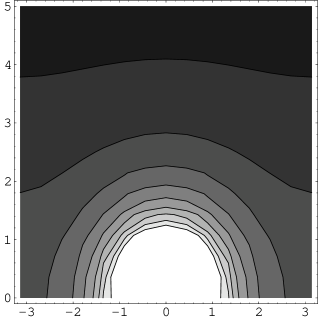
Figure 1: Equipotential lines for $F_{2}(a,b)$ corresponding to $d=4$. Horizontal axis is $b$ and vertical axis is $a$.

As an illustration of the $(R,v)$ coordinate system, we have depicted the equipotential lines for $F_{d-2}$ in Figure 1. Clearly the $v$-coordinate is periodic with period $2\pi$ for large $R$ and not periodic for small $R$. We now find the critical $R$ value where $v$ goes from being periodic to not being periodic. It is clear from Figure 1 that the critical curve that separates $v$ being periodic or not, is the curve that goes through the point $(r=0,z=\pi R_{T})$. Computing the value of $F_{d-2}$ in this point we find

$$F_{d-2}(0,\pi)=\frac{2}{\pi^{d-2}}\left(1-\frac{1}{2^{d-2}}\right)\zeta(d-2)\ .$$ (2.31)

Then using the definition of $R$ (2.15) we obtain the critical value $R_{c}$ of the $R$ coordinate as

$$R_{c}^{d-3}=\frac{1}{2}k_{d}\frac{(2\pi)^{d-2}}{2^{d-2}-1}\frac{1}{\zeta(d-2)}\ .$$ (2.32)

For $R<R_{c}$ we see that $v$ is not periodic and that the range of $v$ is $[-\pi,\pi]$. For $R>R_{c}$ we have that $v$ is periodic with period $2\pi$ and we can for instance choose the range $[-\pi,\pi[$. At the critical value $R=R_{c}$ we see that $v$ is periodic with period $2\pi$, but the coordinate map has a singularity in $v=\pi$, corresponding to the point $(r=0,z=\pi R_{T})$.

2.3 The flat metric

Finally, using the coordinates (2.15), (2.26), (2.27) the flat metric on the $d$-dimensional cylinder $\mathbb{R}^{d-1}\times S^{1}$ can be written as

$$ds_{d}^{2}=R_{T}^{2}\left(A_{(0)}dR^{2}+\frac{A_{(0)}}{(K_{(0)})^{d-2}}dv^{2}+K_{(0)}R^{2}d\Omega_{d-2}^{2}\right)$$ (2.33)

where

$$A_{(0)}=\frac{1}{R_{T}^{2}}\frac{(d-3)^{2}}{k_{d}^{\frac{2}{d-3}}}\frac{F_{d-2}^{2\frac{d-2}{d-3}}}{(\partial_{r}F_{d-2})^{2}+(\partial_{z}F_{d-2})^{2}}$$ (2.34)

$$K_{(0)}=\left(\frac{r}{R_{T}}\right)^{2}\left(\frac{F_{d-2}}{k_{d}}\right)^{\frac{2}{d-3}}\ .$$ (2.35)

It is important to note here that since the functions $r(R,v)$, $F_{d-2}(R,v)$, $\partial_{r}F_{d-2}(R,v)$ and $(\partial_{z}F_{d-2}(R,v))^{2}$ are periodic in $v$ with period $2\pi$, then $A_{(0)}(R,v)$ and $K_{(0)}(R,v)$ are periodic in $v$ with period $2\pi$. Thus, even though $v$ is not a periodic coordinate for $R<R_{c}$ we find that the flat metric (2.33) is periodic in $v$ with period $2\pi$ for all $R$. Note also that the functions $A_{(0)}(R,v)$ and $K_{(0)}(R,v)$, and thereby the flat metric (2.33), are smooth on the space given by $R\in[0,\infty[$ and $v\in\,]-\pi,\pi[$.

From the fact that $A_{(0)}(R,v)$ and $K_{(0)}(R,v)$ are even periodic functions in $v$ with period $2\pi$, follows that we can write the Fourier expansions

$$K_{(0)}(R,v)=\sum_{n=0}^{\infty}\cos(nv)\,L_{0}^{(n)}(R)$$ (2.36)

$$A_{(0)}(R,v)=\sum_{n=0}^{\infty}\cos(nv)\,B_{0}^{(n)}(R)\ .$$ (2.37)

We emphasize that this expansion holds for all $(R,v)$. The functions $L_{0}^{(n)}(R)$ and $B_{0}^{(n)}(R)$ are considered in Appendix C for $n=1,2$, by working out the $(R,v)\leftrightarrow(r,z)$ change of coordinates for large $R$ through second order.

The flat metric (2.33) can be used to write the extremal dilatonic $p$-brane solution (2.6)-(2.8) as

$$ds_{D}^{2} = H^{-\frac{d-2}{D-2}}\left[-dt^{2}+\sum_{i=1}^{p}(dx^{i})^{2}\right.$$ (2.38)

$$\left.+HR_{T}^{2}\left(A_{(0)}dR^{2}+\frac{A_{(0)}}{(K_{(0)})^{d-2}}dv^{2}+K_{(0)}R^{2}d\Omega_{d-2}^{2}\right)\right]$$

$$e^{2\phi}=H^{a}\ \ ,\ \ \ \ A_{01\cdots p}=1-H^{-1}$$ (2.39)

with harmonic function

$$H=1+\frac{h_{d}}{R^{d-3}}\ \ ,\ \ \ \ h_{d}\equiv k_{d}\frac{L^{d-2}}{R_{T}^{d-2}}\ .$$ (2.40)

3 Ansatz

In this section we find an ansatz that we believe can describe non-extremal charged dilatonic branes with a transverse circle. In order to do this, we first make precise what the conditions on such an ansatz should be.

Part of these conditions is to demand that the solution should interpolate between the usual black brane with transverse space $\mathbb{R}^{d}$, which is a good description at small mass, and the black brane smeared on the transverse circle, which is a good description at large mass. We are thus advocating the philosophy that a small black hole on a cylinder can be continuously deformed into a black string wrapped on the cylinder by increasing the mass ad infinitum.

As mentioned before, one of the complications in finding solutions of black holes on the cylinder $\mathbb{R}^{d-1}\times S^{1}$ is that on its covering space $\mathbb{R}^{d}$ the configuration is really a one-dimensional array of black holes. Hence, due to the non-linear nature of the interactions among the black hole, the geometry is expected to be very complicated. On the other hand, it is physically clear that such solutions should exist, at least for small black holes. One could naively think that they would be unstable since on the covering space a slight perturbation of one of the black holes would destroy the array. However, the black holes are constrained to be at a fixed distance which is what removes that instability.

In the literature, only black holes on $\mathbb{R}^{2}\times S^{1}$ have been considered previously [10, 11, 12, 13]. This case is very different from the generic case since the curvature term of the $S^{1}$ symmetry of the $\mathbb{R}^{2}$ in the usual spherical ansatz drops out of the Einstein equations. It is therefore possible in this case to reduce the Einstein equations to exactly solvable linear equations.

The class of black holes we are considering in this section are the singly charged dilatonic black holes that correspond to the $p$-branes of M-theory and Type IIA/IIB String Theory compactified in the longitudinal directions on a $p$-torus. When discussing the solutions we discuss the $p$-brane solutions rather than the compactified black hole solutions (See Appendix A for details on $p$-brane solutions of String and M-theory and for the compactification on $T^{p}$).

We shall see that for this class of black holes it is possible to make an ansatz for the solution that reduces the EOMs (equations of motion) into three equations for one function of two variables. This ansatz is constructed using the new coordinate system found in Section 2, and is tailored to fulfil the appropriate boundary conditions.

3.1 Conditions on a solution

In order to make an ansatz for the solution of dilatonic $p$-branes with transverse space $\mathbb{R}^{d-1}\times S^{1}$ we need to determine the boundary conditions that should be imposed.

As a preliminary, we define a general Schwarzschild radius $R_{0}$ to be the maximal value of the $R$ coordinate on the horizon in the $(R,v)$ coordinates.

We have three types of boundary conditions we want to impose. First, we have the parts of the metric that are independent of the charge of the solution. For these, we impose the boundary conditions:

• The solution reduces to an ordinary black $p$-brane with transverse space $\mathbb{R}^{d}$ when $R_{0}\leq R\ll 1$.

• The solution reduces to a black $p$-brane smeared on the transverse circle when $R\geq R_{0}\gg 1$.

Condition (i) tells us that for small $R_{0}$ we can ignore the size of the transverse circle and regard it as non-compact so that the solution should be the one corresponding to transverse space $\mathbb{R}^{d}$. In $(R,v)$ coordinates, this solution is

$$ds_{D}^{2} = H^{-\frac{d-2}{D-2}}\left[-fdt^{2}+\sum_{i=1}^{p}(dx^{i})^{2}\right.$$ (3.1)

$$\left.+HR_{T}^{2}\left(f^{-1}A_{(0)}dR^{2}+\frac{A_{(0)}}{(K_{(0)})^{d-2}}dv^{2}+K_{(0)}d\Omega_{d-2}^{2}\right)\right]$$

$$e^{2\phi}=H^{a}\ \ ,\ \ \ \ A_{01\cdots p}=\coth\alpha\Big{(}1-H^{-1}\Big{)}$$ (3.2)

$$f=1-\frac{R_{0}^{d-3}}{R^{d-3}}\ \ ,\ \ \ \ H=1+\frac{R_{0}^{d-3}\sinh^{2}\alpha}{R^{d-3}}$$ (3.3)

with

$$A_{(0)}=\left(\frac{d-3}{d-2}\right)^{2}\left(\frac{R_{T}}{k_{d}\rho}\right)^{\frac{2}{d-3}}=\left(\frac{d-3}{d-2}\right)^{2}(k_{d}R)^{-\frac{2}{d-2}}$$ (3.4)

$$K_{(0)}=\frac{\rho^{2}}{R_{T}^{2}}\sin^{2}\theta$$ (3.5)

and $\alpha$ is defined by

$$h_{d}=R_{0}^{d-3}\cosh\alpha\sinh\alpha\ .$$ (3.6)

To obtain this result we used the non-extremal charged dilatonic $p$-brane solution (A.11)-(A.13) and the limiting coordinate transformations $R(\rho)$ and $v(\theta)$ given in (2.17) and (2.30) respectively. This solution is valid in $(R,v)$ coordinates for $R_{0}\leq R\ll 1$.

Condition (ii) says that for large $R_{0}$ we can ignore the coordinate in the circle direction, and thus the solution is that of a $p$-brane smeared in one direction. In $(R,v)$ coordinates, this solution is

$$ds_{D}^{2}=H^{-\frac{d-2}{D-2}}\left[-fdt^{2}+\sum_{i=1}^{p}(dx^{i})^{2}+HR_{T}^{2}\left(f^{-1}dR^{2}+dv^{2}+R^{2}d\Omega_{d-2}^{2}\right)\right]$$ (3.7)

$$e^{2\phi}=H^{a}\ \ ,\ \ \ \ A_{01\cdots p}=\coth\alpha\Big{(}1-H^{-1}\Big{)}$$ (3.8)

$$f=1-\frac{R_{0}^{d-3}}{R^{d-3}}\ \ ,\ \ \ \ H=1+\frac{R_{0}^{d-3}\sinh^{2}\alpha}{R^{d-3}}$$ (3.9)

with $\alpha$ defined again by (3.6). This results follows using the smeared non-extremal charged dilatonic $p$-brane solution in (A.18)-(A.19) and the limiting coordinate transformations $R(r)$ and $v(z)$ given in (2.16) and (2.29) respectively. This solution is valid in $(R,v)$ coordinates for $R\geq R_{0}\gg 1$.

In addition to the two preceding conditions, we want to ensure that the general black solution is the thermally excited version of the extremal charged dilatonic $p$-brane on $\mathbb{R}^{d-1}\times S^{1}$. Hence, we impose the condition:

• For $R_{0}/R\rightarrow 0$ the solution approaches the solution (2.38)-(2.40) corresponding to an extremal dilatonic $p$-brane with transverse space $\mathbb{R}^{d-1}\times S^{1}$.

This condition has several important consequences. First, we see that for $R_{0}=0$ the solution should reduce to the extremal dilatonic $p$-brane with transverse space $\mathbb{R}^{d-1}\times S^{1}$ given by (2.38)-(2.40).

Moreover, if we consider a small $R_{0}$, i.e. a small black hole on a cylinder, the solution should approximately look like the extremal solution (2.38)-(2.40). In Section 5 we take a closer look at the case of small black holes on cylinders.

If we instead consider a fixed $R_{0}$, then condition (iii) has the consequence that for $R/R_{0}\rightarrow\infty$ the solution should approach the extremal solution given by (2.38)-(2.40). This ensures that the reference space of the black hole is the extremal dilatonic $p$-brane on $\mathbb{R}^{d-1}\times S^{1}$ given by (2.38)-(2.40).

A corollary to this last remark is that for a given finite $R_{0}>R_{c}$ the solution cannot be translationally invariant along the circle since for sufficiently large $R$ it has to be approximately equal to the extremal solution (2.38)-(2.40) which is not translationally invariant along the circle. We are thus forced to discard the usual smeared black $p$-brane solution for finite $R_{0}>R_{c}$ as the exact solution. The smeared black $p$-brane solution is only exact for $R_{0}\rightarrow\infty$.

The three preceding conditions are not enough. We need in addition to specify a location of the horizon. We therefore assume the extra condition:

• The horizon is located at constant $R$.

The rationale behind this condition is that the equipotential surfaces of the charge potential are defined by $R$ being constant and we expect the horizon to be at an equipotential surface. Obviously, the horizon is then defined by the equation $R=R_{0}$.

In Section 5 we consider an additional condition on the $g_{00}$ component of the metric for solutions with $R_{0}\ll 1$.

3.2 The ansatz

We are now ready to specify our ansatz for the dilatonic black $p$-brane with transverse space $\mathbb{R}^{d-1}\times S^{1}$. In accordance with the conditions above we write

$$ds_{D}^{2} = H^{-\frac{d-2}{D-2}}\left[-fdt^{2}+\sum_{i=1}^{p}(dx^{i})^{2}\right.$$ (3.10)

$$\left.+HR_{T}^{2}\left(f^{-1}AdR^{2}+Cdv^{2}+KR^{2}d\Omega_{d-2}^{2}\right)\right]$$

$$e^{2\phi}=H^{a}\ \ ,\ \ \ \ A_{01\cdots p}=\coth\alpha\Big{(}1-H^{-1}\Big{)}$$ (3.11)

along with the functions

$$f=1-\frac{R_{0}^{d-3}}{R^{d-3}}\ \ ,\ \ \ \ H=1+\frac{R_{0}^{d-3}\sinh^{2}\alpha}{R^{d-3}}$$ (3.12)

and

$$h_{d}=R_{0}^{d-3}\cosh\alpha\sinh\alpha\ .$$ (3.13)

Here, we introduced the three undetermined functions $A(R,v)$, $C(R,v)$ and $K(R,v)$.

In accordance with condition (iv) above, the equation $R=R_{0}$ defines the horizon of the black hole. The conditions (i)-(iii) above are satisfied provided the functions $A$, $C$ and $K$ reduce to their extremal values if we consider the limit $R_{0}/R\rightarrow 0$ or the limit $R_{0}\gg R_{c}$. Apart from the requirements coming from the conditions, we have also imposed that the metric is diagonal. Though it is not a priori obvious that this is possible, we shall present strong evidence below that this in fact gives consistent EOMs.

We can be even more restrictive in the ansatz for the metric. If we consider the EOM for the field strength

$$\partial_{\mu}(\sqrt{-g}e^{a\phi}F^{\mu\nu})=0$$ (3.14)

we get

$$\partial_{R}\left[\sqrt{\frac{CK^{d-2}}{A}}R^{d-2}\partial_{R}H\right]=0\ .$$ (3.15)

Using (3.12) we see that this requires $CK^{d-2}/A$ to be independent of $R$. It then follows from the boundary conditions above that $C=AK^{-(d-2)}$. The ansatz for charged dilatonic black holes on $\mathbb{R}^{d-1}\times S^{1}$ therefore becomes

$$ds_{D}^{2} = H^{-\frac{d-2}{D-2}}\left[-fdt^{2}+\sum_{i=1}^{p}(dx^{i})^{2}\right.$$ (3.16)

$$\left.+HR_{T}^{2}\left(f^{-1}AdR^{2}+\frac{A}{K^{d-2}}dv^{2}+KR^{2}d\Omega_{d-2}^{2}\right)\right]$$

$$e^{2\phi}=H^{a}\ \ ,\ \ \ \ A_{01\cdots p}=\coth\alpha\Big{(}1-H^{-1}\Big{)}$$ (3.17)

$$f=1-\frac{R_{0}^{d-3}}{R^{d-3}}\ \ ,\ \ \ \ H=1+\frac{R_{0}^{d-3}\sinh^{2}\alpha}{R^{d-3}}$$ (3.18)

$$h_{d}=R_{0}^{d-3}\cosh\alpha\sinh\alpha$$ (3.19)

with only two undetermined functions $A(R,v)$ and $K(R,v)$ at this point. Below we find $A(R,v)$ in terms of $K(R,v)$ so that ultimately the ansatz (3.16)-(3.19) has only one undetermined function $K(R,v)$.

4 Map of solution to neutral and near-extremal solutions

In this section we use the fact that the equations for $A(R,v)$ and $K(R,v)$ are independent of the charge parameter $h_{d}$ to map the ansatz for non-extremal charged dilatonic branes with a transverse circle to an ansatz for neutral black holes on cylinders and to near-extremal charged dilatonic branes with a transverse circle.

4.1 Neutral black holes on a cylinder

It can be checked that the EOMs for the ansatz (3.16)-(3.19) are independent of the constant $h_{d}$ which is proportional to the charge. Thus, the EOMs are the same for a neutral non-dilatonic black hole on $\mathbb{R}^{d-1}\times S^{1}$ with metric

$$ds_{d+1}^{2}=-fdt^{2}+R_{T}^{2}\left[f^{-1}AdR^{2}+\frac{A}{K^{d-2}}dv^{2}+KR^{2}d\Omega_{d-2}^{2}\right]$$ (4.1)

where

$$f=1-\frac{R_{0}^{d-3}}{R^{d-3}}\ .$$ (4.2)

The boundary conditions are then that $A\rightarrow A^{(0)}$ and $K\rightarrow K^{(0)}$ when $R_{0}\rightarrow 0$ or $R_{0}\rightarrow\infty$ for any $R$. These boundary conditions are also natural for this neutral black hole case, as they express the conditions that we want a) the solution to reduce to a black hole solution on $\mathbb{R}^{d}$ for $R_{0}\rightarrow 0$; b) the solution to reduce to a black string solution for $R_{0}\rightarrow\infty$; and finally c) the solution to reduce to the flat space metric on $\mathbb{R}^{d-1}\times S^{1}$ in $(R,v)$ coordinates when $R_{0}=0$ or in the asymptotic region $R/R_{0}\rightarrow\infty$, so that our solution is asymptotically $\mathbb{R}^{d-1}\times S^{1}$ very far away from the black hole.

Consequently, the problem of finding solutions of black dilatonic $p$-brane with transverse space $\mathbb{R}^{d-1}\times S^{1}$ is mapped to the problem of finding neutral black holes on $\mathbb{R}^{d-1}\times S^{1}$.

4.2 Near-extremal branes on transverse circle

The above stated fact that the black hole structure of the solution of a $p$-brane on a transverse circle is independent of the charge, means that we also can map the non-extremal charged dilatonic $p$-brane solutions to the corresponding near-extremal dilatonic $p$-brane solutions with a transverse circle.

The general near-horizon limit of the non-extremal $p$-brane ansatz (3.16)-(3.19) is

$$R_{T}\rightarrow 0\ \ ,\ \ \ \ R\ \mbox{ fixed}\ \ ,\ \ \ \ R_{0}\ \mbox{ fixed}\ \ ,\ \ \ \ \hat{h}_{d}\equiv R_{T}^{2}h_{d}\ \mbox{ fixed}\ .$$ (4.3)

The resulting near-extremal $p$-brane solution is then

$$R_{T}^{-\frac{2(d-2)}{D-2}}ds_{D}^{2} = \hat{H}^{-\frac{d-2}{D-2}}\left[-fdt^{2}+\sum_{i=1}^{p}(dx^{i})^{2}\right.$$ (4.4)

$$\left.+\hat{H}\left(f^{-1}AdR^{2}+\frac{A}{K^{d-2}}dv^{2}+KR^{2}d\Omega_{d-2}^{2}\right)\right]$$

$$R_{T}^{2a}e^{2\phi}=\hat{H}^{a}\ \ ,\ \ \ \ R_{T}^{-2}A_{01\cdots p}=-\hat{H}^{-1}$$ (4.5)

$$f=1-\frac{R_{0}^{d-3}}{R^{d-3}}\ \ ,\ \ \ \ \hat{H}=\frac{\hat{h}_{d}}{R^{d-3}}$$ (4.6)

where the functions $A(R,v)$ and $K(R,v)$ are the same as in the ansatz (3.16)-(3.19). So, as promised, the “black part” of the near-extremal solution is the same as that of the corresponding non-extremal and neutral solutions.

5 Newton limit of small black holes on cylinders

In this section we examine the limit of small black holes on cylinders, i.e. the limit $R_{0}\ll R_{c}$. This is done for two purposes. Firstly, we want to test the ansatz (3.16)-(3.19) in this limit and verify that this case can be correctly incorporated. We find that the results are indeed consistent and that the ansatz (3.16)-(3.19) works in this case. Secondly, we shall see that the results of this section have important consequences for the form of the general solution. We restrict ourselves to the neutral case with ansatz (4.1)-(4.2) in this section but all the results can trivially be extended to the charged case due to the map discussed in Section 4.1.

5.1 The Newton limit of Einsteins equation

We consider Einsteins equations in a $(d+1)$-dimensional space-time,

$$R_{\mu\nu}-\frac{1}{2}g_{\mu\nu}R=8\pi G_{d+1}T_{\mu\nu}\ \ ,\ \ \ \ \mu,\nu=0,1,...,d$$ (5.1)

with a weak gravitational field

$$|g_{\mu\nu}-\eta_{\mu\nu}|\ll 1$$ (5.2)

where $\eta_{\mu\nu}=\mbox{diag}(-1,1,...,1)$ is the Minkowski metric. Other types of flat space coordinates will be considered below. We also impose that the metric is static so that $\partial_{t}g_{\mu\nu}=0$ and $g_{0i}=0$, $i=1,...,d$ and hence $R_{0i}=0$. We consider non-relativistic matter

$$T_{00}=\varrho\ \ ,\ \ \ \ |T_{ij}|\ll\varrho\ \ ,\ i,j=1,...,d$$ (5.3)

where $\varrho$ is the density of mass. From the above equations we find to leading order

$$R^{0}_{\ 0}=-\frac{d-2}{d-1}8\pi G_{d+1}\varrho\ \ ,\ \ \ \ R^{i}_{\ j}=\delta^{i}_{j}\frac{1}{d-1}8\pi G_{d+1}\varrho\ .$$ (5.4)

The Geodesic equation in a weak gravitational field gives to leading order

$$\frac{\partial^{2}x^{i}}{\partial t^{2}}=\frac{1}{2}\partial_{i}g_{00}\ .$$ (5.5)

Comparing with Newtons Second law in a Newton gravitational potential $\Phi$

$$\frac{\partial^{2}x^{i}}{\partial t^{2}}=-\partial_{i}\Phi$$ (5.6)

we identify

$$\partial_{i}g_{00}=-2\partial_{i}\Phi\ .$$ (5.7)

Since $g^{(0)}_{00}=-1$ we then see that we must have

$$g_{00}=-(1+2\Phi)$$ (5.8)

to leading order.

From the definition of the Ricci tensor we have $R^{0}_{\ 0}=\frac{1}{2}\nabla^{2}g_{00}$, where $\nabla^{2}=\partial^{i}\partial_{i}$. Using (5.4) and (5.8), we then find that Newtons equation for the Newton gravitational potential is

$$\nabla^{2}\Phi=8\pi G_{d+1}\varrho\frac{d-2}{d-1}\ .$$ (5.9)

Thus, in terms of the gravitational potential we have the equations

$$R^{0}_{\ 0}=-\nabla^{2}\Phi\ \ ,\ \ \ \ R^{i}_{\ j}=\delta^{i}_{j}\frac{1}{d-2}\nabla^{2}\Phi\ .$$ (5.10)

We can instead consider other flat coordinates so that the metric to leading order can be written

$$g_{\mu\nu}=g^{(0)}_{\mu\nu}+g^{(1)}_{\mu\nu}+\cdots$$ (5.11)

where $g^{(0)}_{\mu\nu}$ is the flat space metric in the coordinates under consideration (with $g^{(0)}_{00}=-1$ and $g^{(0)}_{0i}=0$) and $g^{(1)}_{\mu\nu}$ the leading correction expressed in these new coordinates. In this more general case the equations (5.10) still hold for the metric $g_{\mu\nu}$ to leading order, provided the Laplacian is taken in its covariant form

$$\nabla^{2}\Phi=\frac{1}{\sqrt{-g^{(0)}}}\partial_{\mu}\left(\sqrt{-g^{(0)}}\partial^{\mu}\Phi\right)\ .$$ (5.12)

Clearly, also the relation (5.8) holds for other choices of flat coordinates.

5.2 The Newton potential and the $g_{00}$ component

In this section we describe how the standard connection (5.8) between the $g_{00}$ component of the metric and the Newton potential works for small black holes using the ansatz (4.1)-(4.2).

If we consider a point mass of mass $M$ in flat space $\mathbb{R}^{d}$ we get from the equation for a Newtonian gravitational potential (5.9) that

$$\Phi=-\frac{8\pi G_{d+1}M}{(d-1)\Omega_{d-1}r^{d-2}}\ .$$ (5.13)

If we instead consider a point mass of mass $M$ on the cylinder $\mathbb{R}^{d-1}\times S^{1}$ we obtain using the superposition principle the potential

$$\Phi = -\frac{8\pi G_{d+1}M}{(d-1)\Omega_{d-1}}\sum_{n\in\mathbb{Z}}\frac{1}{(r^{2}+(z+2\pi nR_{T})^{2})^{(d-2)/2}}$$ (5.14)

$$= -\frac{8\pi G_{d+1}M}{(d-1)\Omega_{d-1}R_{T}^{d-2}}F_{d-2}\left(\frac{r}{R_{T}},\frac{z}{R_{T}}\right)\ .$$

Using now the connection (5.8) between $\Phi$ and $g_{00}$ and in the Newtonian limit, we find that

$$g_{00}=-1+\frac{16\pi G_{d+1}M}{(d-1)\Omega_{d-1}R_{T}^{d-2}}F_{d-2}\left(\frac{r}{R_{T}},\frac{z}{R_{T}}\right)$$ (5.15)

for a point mass of mass $M$ on a cylinder $\mathbb{R}^{d-1}\times S^{1}$.

We can now compare with our ansatz (4.1)-(4.2) which has

$$g_{00}=-1+\frac{R_{0}^{d-3}}{R^{d-3}}=-1+R_{0}^{d-3}k_{d}^{-1}F_{d-2}\left(\frac{r}{R_{T}},\frac{z}{R_{T}}\right)\ .$$ (5.16)

We see that the ansatz precisely has the right form of $g_{00}$ to reproduce the gravitational potential (5.14) and (5.15) for $R\gg R_{0}$. That $g_{00}$ should have this form for $R_{0}\ll R_{c}$ is an additional condition for black hole solutions on cylinders independent of the conditions of Section 3.1.

Moreover, by comparing (5.15) and (5.16) we can determine the mass

$$M=\frac{(d-3)(d-1)}{d-2}\frac{\Omega_{d-2}2\pi R_{T}}{16\pi G_{d+1}}(R_{0}R_{T})^{d-3}\ .$$ (5.17)

This shows that the mass $M$ of a small black hole on the cylinder $\mathbb{R}^{d-1}\times S^{1}$ is the same as the mass of a black hole with the same horizon radius $R_{0}$ but in $\mathbb{R}^{d}$ ($\mathbb{R}^{d}$ is obtained if we impose that (2.17) holds exactly for all $R$). This means that the mass of the black hole is not affected by the global structure of the space surrounding it, provided it is sufficiently small. So a black hole obeys the locality principle in this respect. This not a completely trivial result in the sense that energy in General Relativity only can be defined globally. However, this result is to be expected if the weak gravitational region around a black hole should behave like that of Newtonian gravity.

5.3 The metric in the Newton limit

We now want to describe how, given a gravitational potential $\Phi=\Phi(R)$, the leading order correction to the metric is determined. In (5.8) this was given for the $g_{00}$ component. However, this is highly gauge-dependent, so we need to fix the gauge by writing an ansatz for the corrections. Since we want this ansatz to reduce to the weak gravitational field limit of (4.1)-(4.2) when $\Phi=-\frac{1}{2}\frac{R_{0}^{d-3}}{R^{d-3}}$ we write the ansatz

$$ds_{d+1}^{2} = -\Big{(}1+2\Phi\Big{)}dt^{2}+R_{T}^{2}\left[\Big{(}1-2u+2g\Big{)}A_{(0)}dR^{2}\right.$$ (5.18)

$$\left.+\Big{(}1+2g-(d-2)2h\Big{)}\frac{A_{(0)}}{K_{(0)}^{d-2}}dv^{2}+\Big{(}1+2h\Big{)}K_{(0)}R^{2}d\Omega_{d-2}^{2}\right]$$

where $u$, $g$ and $h$ are undetermined functions. The idea is now to find $u$, $g$ and $h$ as functions of $\Phi$ and its derivatives so that the approximate Einstein equations (5.10) are satisfied.

Since the right hand side of (5.10) has at most two derivatives of $\Phi$ we expect that the metric can be written in terms of $\Phi$ and $\Phi^{\prime}$ only, since e.g. a $\Phi^{\prime\prime}$ term in the metric would give $\Phi^{\prime\prime\prime}$ terms or higher in the Ricci tensor. Thus, we should find $u$, $g$ and $h$ as function of $R$, $v$, $\Phi$ and $\Phi^{\prime}$. Clearly they have to be linear combinations of $\Phi$ and $\Phi^{\prime}$ since we only consider leading corrections. For $u$ this has the immediate consequence that

$$u=(1-\lambda)\Phi-\lambda\frac{R}{d-3}\Phi^{\prime}$$ (5.19)

for some function $\lambda=\lambda(R,v)$. This is because we want to impose that $u=-\frac{1}{2}\frac{R_{0}^{d-3}}{R^{d-3}}$ whenever $\Phi=-\frac{1}{2}\frac{R_{0}^{d-3}}{R^{d-3}}$.

The metric for $R\gg R_{c}$

For $R\gg R_{c}$ we have $A_{(0)}=K_{(0)}=1$, so that the ansatz (5.18) becomes

$$ds_{d+1}^{2} = -\Big{(}1+2\Phi\Big{)}dt^{2}+R_{T}^{2}\left[\Big{(}1-2u+2g\Big{)}dR^{2}\right.$$ (5.20)

$$\left.+\Big{(}1+2g-(d-2)2h\Big{)}dv^{2}+\Big{(}1+2h\Big{)}R^{2}d\Omega_{d-2}^{2}\right]\ .$$

From the Einstein equation $(d-2)R^{v}_{\ v}-\nabla^{2}\Phi=0$ we get

$$\nabla^{2}\left[(d-2)h-g-\frac{1}{d-2}\Phi\right]=0\ .$$ (5.21)

Clearly, in order for this to hold for general potentials $\Phi$ we need

$$g=(d-2)h-\frac{1}{d-2}\Phi\ .$$ (5.22)

We now write

$$h=h_{1}\Phi-h_{2}\frac{R}{d-3}\Phi^{\prime}$$ (5.23)

where $h_{1}$ and $h_{2}$ are constants. Using this along with (5.19) with $\lambda$ a constant we find from the remaining Einstein equations $(d-2)R^{R}_{\ R}=\nabla^{2}\Phi$ and $(d-2)R^{\phi_{1}}_{\ \phi_{1}}=\nabla^{2}\Phi$ that $h_{1}=1/((d-2)(d-3))$, $h_{2}=0$ and $\lambda=1$. Thus, we have

$$u=-\frac{R}{d-3}\Phi^{\prime}\ \ ,\ \ \ \ h=\frac{1}{(d-2)(d-3)}\Phi\ \ ,\ \ \ \ g=\frac{1}{(d-2)(d-3)}\Phi$$ (5.24)

which uniquely determines the metric (5.18) in terms of the Newton gravitational potential. However, we have neglected above to explain why we can assume $h_{1}$, $h_{2}$ and $\lambda$ to be constants. As we shall see below at least $h_{1}$ is dependent on $R$. But, since we neglect any correction to the metric of order $\exp(-R)$ our assumption that $h_{1}$, $h_{2}$ and $\lambda$ are constants is really an assumption that they are constants up to corrections of order $\exp(-R)$. This is just another way of saying that we have obtained the leading contribution to $h_{1}$, $h_{2}$ and $\lambda$ for $R\gg R_{c}$.

The metric for $R_{0}\ll R\ll R_{c}$

We now turn to the region $R_{0}\ll R\ll R_{c}$. Here it is convenient to work in the $(\rho,\theta)$ coordinates in terms of which the ansatz (5.18) becomes

$$ds_{d+1}^{2} = -\Big{(}1+2\Phi\Big{)}dt^{2}+R_{T}^{2}\left[\Big{(}1-2u+2g\Big{)}d\rho^{2}\right.$$ (5.25)

$$\left.+\Big{(}1+2g-(d-2)2h\Big{)}\rho^{2}d\theta^{2}+\Big{(}1+2h\Big{)}\rho^{2}\sin^{2}\theta d\Omega_{d-2}^{2}\right]\ .$$

The $R_{\rho\theta}=0$ equation gives $\partial_{\rho}g=(d-1)\partial_{\rho}h$, so that $g=(d-1)h$. This means that the metric is spherically symmetric. All the Einstein equations are then solved if and only if

$$u=(d-2)h-\rho\partial_{\rho}h-\frac{\rho}{d-2}\partial_{\rho}\Phi\ .$$ (5.26)

Since $u=-\frac{1}{2}\frac{\rho_{0}^{d-2}}{\rho^{d-2}}$ whenever $\Phi=-\frac{1}{2}\frac{\rho_{0}^{d-2}}{\rho^{d-2}}$ we see that $h=0$ since the above equation would otherwise determine that $h$ is proportional to $\rho^{d-2}$. Thus, we have

$$u=-\frac{\rho}{d-2}\partial_{\rho}\Phi\ \ ,\ \ \ \ h=g=0$$ (5.27)

which determines the metric (5.25) in this case. In the $(R,v)$ coordinates these relations read

$$u=-\frac{R}{d-3}\Phi^{\prime}\ \ ,\ \ \ \ h=g=0\ .$$ (5.28)

5.4 Consequences for small black hole on cylinder

From (4.1)-(4.2) it follows that the ansatz for a black hole on a cylinder $\mathbb{R}^{d-1}\times S^{1}$ is

$$ds_{d+1}^{2}=-fdt^{2}+R_{T}^{2}\left[f^{-1}AdR^{2}+\frac{A}{K^{d-2}}dv^{2}+KR^{2}d\Omega_{d-2}^{2}\right]$$ (5.29)

$$f=1-\frac{R_{0}^{d-3}}{R^{d-3}}\ .$$ (5.30)

We first observe, as has already been remarked before, that this metric fits into the general ansatz for the Newton limit (5.18) on a cylinder with

$$\Phi=u=-\frac{1}{2}\frac{R_{0}^{d-3}}{R^{d-3}}\ \ ,\ \ \ \ A=A_{(0)}(1+2g)\ \ ,\ \ \ \ K=K_{(0)}(1+2h)\ .$$ (5.31)

The results of Section 5.3 now give the two limiting cases

$$h=g=0 \mbox{for}\;\;R_{0}\ll R\ll R_{c}$$ (5.32)

$$2h=2g=-\frac{1}{(d-2)(d-3)}\frac{R_{0}^{d-3}}{R^{d-3}} \mbox{for}\;\;R\gg R_{c}\ .$$ (5.33)

That $h=g=0$ for $R_{0}\ll R\ll R_{c}$ justifies our condition (i) in Section 3.1 that the solution we consider should reduce to the solution with transverse space $\mathbb{R}^{d}$ when $R_{0}\leq R\ll R_{c}$. Essentially this means that the small black hole is so small that in its close vicinity the cylindrical geometry can be ignored. Again, this can be seen as a reflection of the fact that the black hole obeys the locality principle in the sense that the black hole solution near the black hole is not affected by the asymptotic structure of the space-time.

That $h$ and $g$ are given by (5.33) for $R\gg R_{c}$ means that the black hole on a cylinder has a potential term in the metric at infinity. This term expresses the attraction of the black hole to itself across the cylinder. Moreover, in the following section we shall see that this term is needed in order to compute the right value for the mass. This is thus another consistency check on our ansatz (3.16)-(3.19).

5.5 Consequences for measurements of mass

We have already seen how to compute the mass of the black hole solution via the $g_{00}$ component in Section 5.2. In this section we test our above results for the Newton limit of the metric on the cylinder $\mathbb{R}^{d-1}\times S^{1}$ by measuring the mass via the Hawking-Horowitz mass formula [20]

$$M=-\frac{1}{8\pi G_{d+1}}\int\frac{d\Omega}{\sqrt{g_{\Omega}}}\int^{2\pi}_{0}dvN\sqrt{g_{d-1}}(K-K_{0})\Big{|}_{R=R_{m}}\ .$$ (5.34)

Here we have evaluated the mass at $R=R_{m}\gg R_{0}$. $N$ is the lapse function which is the extremal value of $\sqrt{-g_{00}}$ which for the case at hand is equal to one. $\sqrt{g_{d-1}}$ is the square root of the metric on the space of constant $t$ and $R=R_{m}$. $K$ is the extrinsic curvature given by

$$K=\frac{\left(\sqrt{g_{d-1}}\right)^{\prime}}{\sqrt{g_{d}}}$$ (5.35)

where $\sqrt{g_{d}}$ is the square root of the metric on the space of $R=R_{m}$. $K_{0}$ is the extremal value of $K$. In terms of the metric (5.18) the mass (5.34) becomes

$$M=\frac{\Omega_{d-2}}{8\pi G_{d+1}}R_{T}^{d-2}R_{m}^{d-2}\int^{2\pi}_{0}dv\left[-g^{\prime}-u\left(\frac{1}{2}\frac{A_{(0)}^{\prime}}{A_{(0)}}+\frac{d-2}{R_{m}}\right)\right]\ .$$ (5.36)

We now evaluate this mass for the small black hole on the cylinder. From (5.31) we know we should set $\Phi=u=-\frac{1}{2}\frac{R_{0}^{d-3}}{R^{d-3}}$. We also calculate

$$\frac{1}{2\pi}\int^{2\pi}_{0}dv\frac{1}{2}\frac{A_{(0)}^{\prime}}{A_{(0)}}=\left\{\begin{array}[]{ccc}-\frac{1}{d-2}\frac{1}{R}&\mbox{ for }&R_{0}\ll R\ll R_{c}\\ 0&\mbox{ for }&R\gg R_{c}\end{array}\right.$$ (5.37)

where we used (3.4), while using (5.32), (5.33) we have that

$$g^{\prime}=\left\{\begin{array}[]{ccc}0&\mbox{ for }&R_{0}\ll R\ll R_{c}\\ \frac{1}{2(d-2)}\frac{1}{R}\frac{R_{0}^{d-3}}{R^{d-3}}&\mbox{ for }&R\gg R_{c}\ .\end{array}\right.$$ (5.38)

Putting (5.37) and (5.38) into (5.36) we obtain for both $R_{0}\ll R_{m}\ll R_{c}$ and $R_{m}\gg R_{c}$ the mass

$$M=\frac{(d-3)(d-1)}{d-2}\frac{\Omega_{d-2}2\pi R_{T}}{16\pi G_{d+1}}(R_{0}R_{T})^{d-3}\ .$$ (5.39)

Since this is the same result as (5.17), we have successfully checked that our Newton limit results are consistent with the mass measured at $R_{0}\ll R\ll R_{c}$ or $R\gg R_{c}$.

One can also put the results (5.24) and (5.28) of Section 5.3 into (5.36) and verify that for both $R_{0}\ll R_{m}\ll R_{c}$ and $R_{m}\gg R_{c}$ we get the same result in terms of the potential $\Phi$.

6 Finding solutions

6.1 Equations of motion

We now find the EOMs for the ansatz (3.16)-(3.19). As stated above, these can be found directly from the metric (4.1) of a neutral non-dilatonic black hole on $\mathbb{R}^{d-1}\times S^{1}$. The EOMs are then given by $R_{\mu\nu}=0$. We get four non-trivial EOMs, $R_{RR}=0$, $R_{vv}=0$ , $R_{Rv}=0$ and $R_{\phi_{1}\phi_{1}}=0$. These four EOMs are

$$0 = (R^{d-3}-R_{0}^{d-3})\Big{[}Ra^{\prime\prime}-(d-2)(Rk^{\prime}+1)a^{\prime}+\frac{1}{2}(d-2)((d-1)Rk^{\prime}+4)k^{\prime})\Big{]}$$ (6.1)

$$+e^{(d-2)k}R^{d-2}((d-2)\dot{a}\dot{k}+\ddot{a})$$

$$0 = (R^{d-3}-R_{0}^{d-3})R(a^{\prime\prime}-(d-2)k^{\prime\prime})+((d-2)R^{d-3}-R_{0}^{d-3})(a^{\prime}-(d-2)k^{\prime})$$ (6.2)

$$+e^{(d-2)k}R^{d-2}\Big{(}\ddot{a}+(d-2)\ddot{k}+\frac{1}{2}(d-1)(d-2)\dot{k}^{2}\Big{)}$$

$$0 = (R^{d-3}-R_{0}^{d-3})\Big{(}R[\dot{k}a^{\prime}+(\dot{a}-(d-1)\dot{k})k^{\prime}-2\dot{k}^{\prime}]-2\dot{k}\Big{)}$$ (6.3)

$$+\frac{1}{(d-2)}\Big{(}2(d-2)R^{d-3}-(d-1)R_{0}^{d-3}\Big{)}\dot{a}$$

$$0 = (R^{d-3}-R_{0}^{d-3})Rk^{\prime\prime}+((d-2)R^{d-3}-R_{0}^{d-3})k^{\prime}$$ (6.4)

$$+e^{(d-2)k}R^{d-2}(\ddot{k}+(d-2)\dot{k}^{2})+2(d-3)R^{d-4}(1-e^{a-k})$$

here written in terms of the functions $a(R,v)$ and $k(R,v)$ defined by

$$A(R,v)=\exp(a(R,v))\ \ ,\ \ \ \ K(R,v)=\exp(k(R,v))\ .$$ (6.5)

We now see from (6.4), which comes from $R_{\phi_{1}\phi_{1}}=0$, that we can find $A(R,v)$ in terms of $K(R,v)$ as

$$A = e^{k}+\frac{e^{k}}{2(d-3)R^{d-4}}\Big{[}(R^{d-3}-R_{0}^{d-3})Rk^{\prime\prime}+((d-2)R^{d-3}-R_{0}^{d-3})k^{\prime}$$ (6.6)

$$+e^{(d-2)k}R^{d-2}(\ddot{k}+(d-2)\dot{k}^{2})\Big{]}\ .$$

This means the Ansatz (3.16)-(3.19) only has one unknown function $K(R,v)$. We can then substitute (6.6) in (6.1)-(6.3) and thereby we obtain three equations for $K(R,v)$ . Due to the complexity of the three equations we have not been able to show that they pose a consistent integrable set of equations. However, in Section 6.3 we show that they are consistent to second order when making an expansion of $K(R,v)$ for large $R$. Moreover, we consider the three equations on the horizon in Section 7.1 and show consistency also in that case.

6.2 General considerations

In the previous section we established that the solution is determined by only one function $K(R,v)$ and that the EOMs gave three equations determining this function. Here we comment on the boundary conditions we put on $K(R,v)$ and we also provide an argument for existence of solutions with $R_{0}>R_{c}$ that are non-translationally invariant along the $z$ direction.

The condition (iii) of Section 3.1 can now be formulated as

$$K(R,v)\rightarrow K_{(0)}(R,v)\ \ \mbox{for}\ \ \frac{R_{0}}{R}\rightarrow 0\ .$$ (6.7)

This means that $K(R,v)$ should have an expansion in powers of $R_{0}^{d-3}/R^{d-3}$ with $K_{(0)}(R,v)$ being the zeroth order term.

In Section 2.3 we established that the flat metric in $(R,v)$ coordinates is periodic for all $v$, even when $R\leq R_{c}$. We therefore impose this on the full non-extremal solution. Thus, $K(R,v)$ is required to be periodic in $v$ with period $2\pi$ for all $R$ and $R_{0}$. Moreover, since $K_{(0)}(R,v)$ is an even function with respect to $v$ we also impose that on the general $K(R,v)$ function.

These two conditions on $K(R,v)$ follow from symmetry arguments. That $K(R,v)$ should be even in $v$ originates from the fact that we want the space-time to be symmetric around $v=0$. Since the metric is a measure of distance this means it has to be even under $v\rightarrow-v$, and hence $K(R,v)$ should be even. The periodicity of the metric for $R<R_{c}$ is then the statement that $K(R,v)$ is the same for $v=\pi$ and $v=-\pi$ and this in fact follows from the fact that $K(R,v)$ is even.

That $K(R,v)$ is an even periodic function of $v$ with period $2\pi$ means we can make a Fourier expansion of $K(R,v)$ as

$$K(R,v)=\sum_{n=0}^{\infty}\cos(nv)\,L^{(n)}(R)\ .$$ (6.8)

For $K_{(0)}(R,v)$ we have from Section 2.3 that

$$K_{(0)}(R,v)=\sum_{n=0}^{\infty}\cos(nv)\,L_{0}^{(n)}(R)\ .$$ (6.9)

Thus we require from (6.7) that $L^{(n)}(R)\rightarrow L_{0}^{(n)}(R)$ for $R_{0}/R\rightarrow 0$.

To further clarify the boundary conditions on $K(R,v)$ we consider the expansion of $L^{(n)}(R)$ for $R\gg 1$. For $K_{(0)}(R,v)$ we have from Appendix C that

$$L_{0}^{(n)}(R)=\sum_{m=0}^{\infty}e^{-(n+2m)R}\,\tilde{L}_{0}^{(n,m)}(R)\ \ ,\ \ \ \ \tilde{L}_{0}^{(0,0)}=1$$ (6.10)

for $R\gg 1$. In analogy with this we define the functions $\tilde{L}^{(n,m)}(R)$ by

$$L^{(n)}(R)=\sum_{m=0}^{\infty}e^{-(n+2m)R}\,\tilde{L}^{(n,m)}(R)\ .$$ (6.11)

That (6.11) is a warranted expression will be clear from the analysis of Section 6.3.

Apart from the boundary condition (6.7) that we already discussed we can now formulate a second crucial boundary condition, namely that

$$\tilde{L}^{(0,0)}(R)=1-\chi(R_{0})\frac{R_{0}^{d-3}}{R^{d-3}}\ .+\cdots$$ (6.12)

This means that for $R\gg 1$ the leading correction to $K(R,v)$ with respect to $K_{(0)}(R,v)$ is precisely that term, so we can also write

$$K(R,v)=1-\chi(R_{0})\frac{R_{0}^{d-3}}{R^{d-3}}\ .+\cdots$$ (6.13)

This is how we impose $K(R,v)$ to behave at $R\rightarrow\infty$. We expect this to be the right type of behavior of $K(R,v)$ for $R\rightarrow\infty$ from the fact we have a term like that for $R_{0}\ll R_{c}$, as explained in Section 5.4.

In some sense the function $\chi(R_{0})$ contains all physical information about the solution, for example the entire thermodynamics can be derived from it as will be explained in Section 7.2. We do not at present know $\chi(R_{0})$, though we know the limiting values

$$\chi(R_{0})=\left\{\begin{array}[]{ccc}\frac{1}{(d-2)(d-3)}&\mbox{for}&R_{0}\ll R_{c}\\ 0&\mbox{for}&R_{0}\gg R_{c}\end{array}\right.$$ (6.14)

where the $R_{0}\ll R_{c}$ value was obtained in Section 5.4. However, as will be clarified in Section 6.3, our expansion (6.11) means that $K(R,v)$ is now in principle completely determined for a given value of $\chi(R_{0})$.

We note that from (6.13) and (6.6) we find

$$A(R,v)=1-\chi(R_{0})\frac{R_{0}^{d-3}}{R^{d-3}}+\cdots$$ (6.15)

as the leading correction with respect to $A_{(0)}(R,v)$ for $R\gg 1$. This is of course consistent with (5.31) and (5.32), (5.33).

Existence of solutions with $R_{0}>R_{c}$

We are now in the position to argue for the existence of solutions with $R_{0}>R_{c}$. Such solutions would necessarily be non-translationally invariant along $z$, but the horizon for such a solution clearly connects to itself across the cylinder. These solutions, if they exist, are thus a new class of solutions that are neither black holes nor black strings.

The argument is simple. On general physical ground it is safe to assume that solutions exist for which $R_{0}<R_{c}$. This is because these solutions just correspond to black holes on a $\mathbb{R}^{d-1}\times S^{1}$ cylinder. Indeed, we have seen in Section 5 that our ansatz (3.16)-(3.19) seems to be able to describe black holes on cylinders. Thus, the question is now whether there are any fundamental differences in solving the EOMs for $R_{0}<R_{c}$ and $R_{0}>R_{c}$. The answer is no. The boundary conditions are the same, $K(R,v)$ is periodic and even function of $v$ and the only difference between small and large $R_{0}$ is in the value of $\chi(R_{0})$. This is just a boundary condition at infinity which means the EOMs should have solutions for any value of $\chi(R_{0})$, as will be further supported in Section 6.3.

Therefore, it seems that in our description there is no fundamental difference in solving the EOMs for $R_{0}<R_{c}$ and $R_{0}>R_{c}$ and the fact that black holes on cylinders exist means that solutions with $R_{0}>R_{c}$ also should exist.

Alternatively, if the statement of existence and uniqueness stated below in Section 6.3 is true (we can only partly verify it) we trivially have that these solutions exist.

6.3 Analysis of equations of motion

In order to clarify the preceding section, we summarize here the boundary conditions and make a statement about existence and uniqueness of solutions that will be justified below.

As shown in Section 6.1 we have three equations for $K(R,v)$. We also recall that $K(R,v)$ completely determines the solution (3.16)-(3.19). Consider now any given value of $R_{0}$ and $\chi$ (we treat $R_{0}$ and $\chi$ as independent parameters in this section). The full set of boundary conditions is then

• $K(R,v)$ is an even periodic function in $v$ with period $2\pi$.

• The Fourier components $L^{(n)}(R)$ of $K(R,v)$ obey

  $$\frac{L^{(n)}(R)}{L_{0}^{(n)}(R)}\rightarrow 1\ \ \mbox{for}\ \ \frac{R_{0}}{R}\rightarrow 0$$ (6.16)

• For $R$ much greater than both $1$ and $R_{0}$ we have

  $$K(R,v)=1-\chi\frac{R_{0}^{d-3}}{R^{d-3}}+\cdots$$ (6.17)

Our general statement about existence and uniqueness is then

• For any given value of $R_{0}$ and any given value of $\chi\geq 0$ the three equations for $K(R,v)$ have a solution obeying the above three boundary conditions and this solution is unique.

The justification of this statement is the subject of the rest of this section.

We start by considering the expression (6.11), which implies that the equations of motion allow a well-defined expansion in terms of powers of the “expansion parameter” $e^{-R}$. First, using (6.8), (6.11) in the expression (6.6) for $A(R,v)$, implies that this function can similarly be written as

$$A(R,v)=\sum_{n=0}^{\infty}\cos(nv)\,B^{(n)}(R)$$ (6.18)

$$B^{(n)}(R)=\sum_{m=0}^{\infty}e^{-(n+2m)R}\,\tilde{B}^{(n,m)}(R)\ .$$ (6.19)

To see that (6.8), (6.11) and (6.18), (6.19) are consistent with the remaining three EOMs (6.1)-(6.3), can be established by induction. Here, the two central ingredients are the specific forms of the EOMs, i.e. the way the $R$ and $v$ derivatives occur, along with standard multiplicative properties of $\cos(mv)$ and $\sin(nv)$.

For example, looking at (6.3), one observes the structures $\dot{z}$, $\dot{z}^{\prime}$ and $\dot{z}z^{\prime}$, where $z$ stands for $a$ or $k$. Thus, the expansions given above generate terms like $\sin(nv)$ and $\sin(nv)\cos(mv)\simeq\sin((n+m)v)+\sin((n-m)v)$. The latter relation is responsible for the fact that (6.11), (6.19) have even shifts $2m$ in the exponential. Then, using induction, it is not difficult to establish the consistency of our proposed expansion. The other two EOMs (6.1), (6.2) can be examined similarly.

Moreover, the expansions (6.8), (6.11) and (6.18), (6.19) are also strongly suggested by the fact that they hold in particular for the extremal functions $K_{(0)}$ and $A_{(0)}$ (see Appendix C). Finally, we explicitly show below the consistency of the truncation by considering the first terms in the expansion.

Using (6.11) the first three terms in $K(R,v)$ take the form

$$K(R,v) = \tilde{L}^{(0,0)}(R)+\cos(v)e^{-R}\tilde{L}^{(1,0)}(R)$$ (6.20)

$$+e^{-2R}[\cos(2v)\tilde{L}^{(2,0)}(R)+\tilde{L}^{(0,1)}(R)]+{\cal{O}}(e^{-3R})$$

$$\equiv y(R)+\cos(v)b(R)+\cos(2v)q(R)+p(R)+{\cal{O}}(e^{-3R})$$ (6.21)

where, for simplicity of notation, we have defined the functions $y(R)$, $b(R)$, $q(R)$ and $p(R)$ in the second line. We now examine the EOMs that arise from substituting these first terms in the expansion. Here and in the following we always implicitly assume that the solution (6.6) for $A(R,v)$ is substituted in (6.1)-(6.3). Moreover, it turns out that there exists a linear combination of the two equations (6.1) and (6.2) that gives rise to a simpler equation (with only up to 3rd order $R$-derivatives of $K(R,v)$), which is given by the difference of these two equations. To facilitate the discussion, we denote the resulting three EOMs symbolically by ${\cal{E}}_{i=1,2,3}$ with

$${\cal{E}}_{1}: \;\;\;R_{Rv}(A(K))=0$$ (6.22)

$${\cal{E}}_{2}: \;\;\;R_{RR}(A(K))-R_{vv}(A(K))=0$$ (6.23)

$${\cal{E}}_{3}: \;\;\;R_{RR}(A(K))=0$$ (6.24)

where the argument $A(K)$ expresses the fact that we have substituted (6.6), and we recall that the Ricci components $R_{RR}$, $R_{vv}$, $R_{Rv}$ are the right hand sides in (6.1), (6.2) and (6.3) respectively. As some of the details become rather involved we will describe the resulting structure below, leaving most of the details to Appendix D. This appendix also gives the corresponding expressions of the expansion of $A(R,v)$ that follow from substituting (6.21) in (6.6).

Starting with the leading $v$-independent term $y(R)=\tilde{L}^{(0,0)}(R)$ in (6.21), it is immediately clear from (6.3) that ${\cal{E}}_{1}$ is satisfied, leaving us with the two equations ${\cal{E}}_{2,3}$. We first analyze ${\cal{E}}_{2}$, which to leading order gives a non-linear differential equation on $y(R)$ which is quartic in $y$ and its derivatives and contains up to three derivatives

$$\sum_{0\leq k\leq l\leq m\leq n\leq 3}c_{klmn}y_{k}y_{l}y_{m}y_{n}=0\ \ ,\ \ \ \ y_{m}\equiv R^{m}\frac{\partial^{m}y(R)}{\partial R^{m}}\ .$$ (6.25)

The ten non-zero coefficients $c_{klmn}$ which are functions of $x=R_{0}/R$ and $d$ are given in (D.6)-(D.15). This differential equation can be solved perturbatively for $R\gg R_{0}$ by substituting the power series expansion

$$y(R)=\tilde{L}^{(0,0)}(R)=1+\sum_{n=1}^{\infty}\alpha_{n}\left(\frac{R_{0}}{R}\right)^{(d-3)n}\ \ ,\ \ \ \ \alpha_{1}=-\chi\ .$$ (6.26)

It turns out that the resulting solution is uniquely determined given $\chi$. In (D.18)-(D.22) we have given the explicit expressions for $\alpha_{n}$, $1\leq n\leq 5$ in terms of $\chi$ for arbitrary $d$. To verify consistency, we still need to consider the remaining EOM ${\cal{E}}_{3}$. Indeed, it turns out that the solution (6.26) of ${\cal{E}}_{2}$ also solves ${\cal{E}}_{3}$. This is the first important non-trivial check of our system of EOMs. In all, we see that up to this point in the expansion we have indeed verified the form (6.17) of $K(R,v)$ for $R\gg 1,R_{0}$ and the claim that the solution is unique given $R_{0}$ and $\chi$.

We continue by studying the first exponentially suppressed correction to $y(R)$, i.e. the $b(R)$-term in (6.21). Starting again with the EOM ${\cal{E}}_{1}$, we now find a second order homogeneous differential equation on $b(R)$

$$M_{0}(R,y(R))b(R)+M_{1}(R,y(R))Rb^{\prime}(R)+M_{2}(R,y(R))R^{2}b^{\prime\prime}(R)=0$$ (6.27)

where the coefficients $M_{m=0,1,2}$ depend on $y(R)$ and its derivatives. The explicit form of this differential equation is given in (D.23). Though the algebra is highly non-trivial, we have explicitly checked that the two equations on $b(R)$ resulting from the other two EOMs, ${\cal{E}}_{2}$ and ${\cal{E}}_{3}$ (which are in fact 3rd and 4th order homogeneous differential equations on $b(R)$ with $y(R)$-dependent coefficients) are indeed satisfied given the $y$-equation (6.25) and the $b$-equation (6.27). Again, this is a rather non-trivial check on the consistency of our system.

Two remarks are in order here. First, since $y(R)$ is uniquely determined given $(R_{0},\chi)$, the equation on $b(R)$ is uniquely determined given $(R_{0},\chi)$. Second, the two boundary conditions that need to be fixed in order to integrate the second order system (D.23) are fixed as a consequence of the boundary conditions (6.16). Indeed, this condition (for $n=1$) represents a boundary condition on $b(R)$ and, by differentiation of (6.16) also its first derivative. In conclusion, we have verified the claim at the beginning of this section to (and including) first order in $e^{-R}$.

Our final explicit computation involves the second order corrections $q(R)$ and $p(R)$ in (6.21). We first discuss $q(R)$ in which case we obtain from ${\cal{E}}_{1}$ a second order inhomogeneous differential equation with $y(R)$-dependent coefficients (as in the $b(R)$ equation). The inhomogeneous part is quadratic in $b(R)$ (and its derivatives). This equation is given in (D.28). Just as for the $b(R)$ equation, we have explicitly checked that the two equations on $q(R)$ resulting from the other two EOMs, ${\cal{E}}_{2}$ and ${\cal{E}}_{3}$ (which are again 3rd and 4th order) are indeed satisfied given the $y$-equation (6.25), the $b$-equation (6.27) and the $q$-equation (D.28).

Turning to $p(R)$, since this is the order $e^{-2R}$ correction to the $v$-independent leading term $y(R)$, we have again that ${\cal{E}}_{1}$ is immediately satisfied. Consequently, the first non-trivial equation results from ${\cal{E}}_{2}$, which gives a third order inhomogeneous differential equation (of similar form as the one for $q(R)$). This equation is given in (D.35). Again, we have verified the non-trivial fact that the other fourth order inhomogeneous differential equation on $p(R)$ coming from ${\cal{E}}_{3}$ is satisfied given the $y$-equation (6.25), $b$-equation (6.27) and the $p$-equation (D.35).

To summarize, our perturbative analysis above has explicitly shown the validity of the expansion (6.11) up to (and including) second order (i.e. to order $e^{-2R}$). We have checked explicitly that the EOMs (6.1)-(6.4), under the boundary conditions given in the beginning of this section, are consistent to this order. We note that some highly non-trivial cancellations in the EOMs were necessary in checking that all three EOMs ${\cal{E}}_{1}$-${\cal{E}}_{3}$ give equations for $y(R)$, $b(R)$, $p(R)$ and $p(R)$ that are mutually consistent. We have thus provided calculational support to our claim above concerning existence and uniqueness of solutions for EOMs corresponding to the ansatz (3.16)-(3.19).

7 Thermodynamics

7.1 Properties of the horizon

We now examine some of the properties of the $R=R_{0}$ hypersurface in the solution given by the ansatz (3.16)-(3.19).

It is clear that when $R_{0}<R_{c}$ the horizon has topology $S^{d-1}$, while for $R_{0}>R_{c}$ the horizon overlaps with itself on the cylinder and has therefore the topology $S^{d-2}\times S^{1}$. For $R_{0}=R_{c}$ the horizon precisely touches itself in one point. If we think about the covering space with an array of black holes, the picture is also clear: For $R_{0}<R_{c}$ the black holes are separated, for $R_{0}=R_{c}$ their horizon touches in one point and for $R_{0}>R_{c}$ the horizons have merged.

If we consider the family of hypersurfaces $R=\mbox{\sl constant}$ then the normal vector is $\frac{\partial}{\partial R}$. Since this vector has zero norm on the horizon (provided $A(R,v)$ is not zero) it follows that the $R=R_{0}$ hypersurface is a null hypersurface. Clearly, it is also a Killing horizon with respect to the Killing vector $\frac{\partial}{\partial t}$ and also with respect to the angular Killing vectors of the $S^{d-2}$ sphere.

Since we have a Killing horizon we can consider the surface gravity $\kappa$. Using $\frac{\partial}{\partial t}$ as the Killing vector, this is computed to be

$$\kappa^{2}=-\frac{1}{4}\lim_{R\rightarrow R_{0}}\Big{[}g^{tt}g^{RR}(\partial_{R}g_{tt})^{2}\Big{]}=\frac{(d-3)^{2}}{4R_{0}^{2}R_{T}^{2}\cosh^{2}\alpha\,A|_{R=R_{0}}}\ .$$ (7.1)

Thus, in order for the surface gravity $\kappa$ to be constant on the horizon, we need $A(R,v)$ to be independent of $v$ on the horizon, i.e. we need $\dot{A}=0$. Fortunately, this follows from the equations of motion (6.1)-(6.4), as we now shall see.

However, we first need to discuss the behavior of $A(R,v)$ and $K(R,v)$ on the horizon. From Section 3.1 we see that $A(R,v)$ and $K(R,v)$ are non-singular on the horizon in the $R_{0}\ll R_{c}$ and $R_{0}\gg R_{c}$ limits. We also know that the flat metric (2.33) is non-singular on the space given by $R\in[0,\infty[$ and $v\in\,]-\pi,\pi[$. We therefore assume that for all values of $R_{0}$ the functions $A(R,v)$ and $K(R,v)$ are non-singular on the horizon for $v\in\,]-\pi,\pi[$.

Under this assumption, the four equations of motion (6.1)-(6.4) reduce for $R=R_{0}$ to the following two equations

$$\dot{a}=0$$ (7.2)

$$e^{a}=e^{k}+\frac{1}{2}R_{0}e^{k}k^{\prime}+\frac{R_{0}^{2}}{2(d-3)}e^{(d-1)k}\left(\ddot{k}+(d-2)\dot{k}^{2}\right)$$ (7.3)

so that we indeed have $\dot{A}=0$, as desired.

Clearly we can combine the two equations (7.2) and (7.3) into one equation for $k$. We thus see that the three equations for $K(R,v)$ reduce to one equation on the horizon and they are therefore a consistent system of differential equations in this limit.

7.2 Thermodynamics

In this section we consider the thermodynamics of non-extremal charged dilatonic $p$-branes that follows from the ansatz (3.16)-(3.19). We also consider the near-extremal and neutral cases.

First we define the function

$$\gamma(R_{0})\equiv\frac{1}{\sqrt{A|_{R=R_{0}}}}$$ (7.4)

which will play an essential role in the thermodynamics. We note the limiting cases

$$\gamma(R_{0})=\left\{\begin{array}[]{ccc}\frac{d-2}{d-3}(k_{d}R_{0})^{\frac{1}{d-2}}&\mbox{for}&R_{0}\ll R_{c}\\ 1&\mbox{for}&R_{0}\gg R_{c}\end{array}\right.$$ (7.5)

as found using (3.4) and (3.7) respectively.

We established in Section 7.1 that the surface gravity $\kappa$ is constant on the horizon. This means we have a well-defined temperature $T$ given as $2\pi T=\kappa$. In particular, from (7.1) and (7.4) we find

$$T=\gamma(R_{0})\frac{d-3}{4\pi R_{0}R_{T}\cosh\alpha}\ .$$ (7.6)

We note that we obtain the same result by Wick rotating the metric (3.16) and demanding absence of a conical singularity near $R=R_{0}$.

Using the Bekenstein-Hawking formula for entropy as the horizon area divided by $4G$ we get the entropy

$$S=\frac{1}{\gamma(R_{0})}\frac{V_{p}\Omega_{d-2}2\pi R_{T}}{4G}(R_{0}R_{T})^{d-2}\cosh\alpha\ .$$ (7.7)

Note that from (7.6) and (7.7) one has

$$TS=\frac{V_{p}\Omega_{d-2}2\pi R_{T}}{16\pi G}(d-3)(R_{0}R_{T})^{d-3}$$ (7.8)

so that the product $TS$ is independent of the function $\gamma(R_{0})$.

The chemical potential $\nu$ and charge $Q$ are given by

$$\nu=\tanh\alpha$$ (7.9)

$$Q=\frac{V_{p}\Omega_{d-2}2\pi R_{T}}{16\pi G}(d-3)(R_{0}R_{T})^{d-3}\cosh\alpha\sinh\alpha\ .$$ (7.10)

Finally, the mass is computed from the Hawking-Horowitz mass formula [20] which we considered in Section 5.5. Using as input the behavior (6.15) of $A(R,v)$ for $R\gg 1$ we find in this case

$$M=\frac{V_{p}\Omega_{d-2}2\pi R_{T}}{16\pi G}(d-3)(R_{0}R_{T})^{d-3}\left[\frac{d-2}{d-3}-\chi(R_{0})+\sinh^{2}\alpha\right]$$ (7.11)

where $\chi(R_{0})$ is defined and discussed in Section 6.2.

For $R_{0}\ll R_{c}$ the thermodynamics (7.6)-(7.7), (7.9)-(7.11) becomes the usual thermodynamics of non-extremal charged dilatonic $p$-branes given in Appendix A. For $R_{0}\gg R_{c}$ it reduces to the usual thermodynamics of non-extremal charged dilatonic $p$-branes smeared in one direction.

The first law of thermodynamics is

$$dM=TdS+\nu dQ$$ (7.12)

Using the above formulas we see that (7.12) holds if and only if $\gamma(R_{0})$ and $\chi(R_{0})$ are related by

$$R_{0}\frac{\gamma^{\prime}}{\gamma}=(d-3)\chi+R_{0}\chi^{\prime}$$ (7.13)

where prime denotes a derivative with respect to $R_{0}$. Using (6.14) and (7.5) we see that this is fulfilled for both $R_{0}\ll R_{c}$ and $R_{0}\gg R_{c}$ provided we take $\chi^{\prime}(R_{0})=0$ in both limits. The formula (7.13) relates the metric at the horizon to the metric for $R\rightarrow\infty$.

Smooth interpolation

As mentioned previously, we are in this paper advocating the idea that there should be a smooth interpolation between the small and large black hole solution on a cylinder. For the thermodynamics, this means that the functions $\gamma(R_{0})$ and $\chi(R_{0})$ should interpolate smoothly between the two limiting cases $R_{0}\ll R_{c}$ and $R_{0}\gg R_{c}$. If we consider $\gamma(R_{0})$ this seems very likely in that $\gamma(R_{0})$ is a concave function for $R_{0}\ll R_{c}$ since the second derivative $\gamma^{\prime\prime}(R_{0})$ is negative at $R_{0}=0$. This fits nicely with the expectation that $\gamma(R_{0})$ should go from from $0$ to $1$ as $R_{0}$ increases from $0$ to $\infty$. Equivalently, the fact that $\chi^{\prime}(R_{0})$ should go to zero for both $R_{0}\rightarrow 0$ and $R_{0}\rightarrow\infty$ fits nicely with the expectation that $\chi(R_{0})$ monotonically decreases from $1/((d-2)(d-3))$ to $0$ as $R_{0}$ increases from $0$ to $\infty$.

We expect that $\chi(R_{0})$ and $\gamma(R_{0})$, and thereby the thermodynamics, are smooth functions of $R_{0}$ because if we consider the metric for $R\geq 0$ and $v\in\,]-\pi,\pi[$ there is no difference between $R\leq R_{c}$ and $R>R_{c}$. We have the same periodicity properties with respect to $v$ and the horizon can smoothly go from $R<R_{c}$ to $R>R_{c}$. Note that we can consistently ignore the set of measure zero defined by $v=\pi$. This is because the boundary conditions of Section 6.3 are not affected by this, so that the EOMs can be solved consistently without including the set $v=\pi$.

However, when we consider the solution in the physical $(r,z)$ coordinates on the cylinder, we have a naked singularity at the event horizon when $R_{0}=R_{c}$. This naked singularity precisely appears when the horizon shifts topology. The singularity is similar to a black hole evaporation effect since in the slice $z=\pi$ it looks like an evaporating black hole. Because of this it seems likely that a small burst of energy will be released which means that the thermodynamics will experience a first order transition at this point. However, for macroscopic cylinders this discontinuity in the thermodynamics at $R_{0}=R_{c}$ will be negligible and it should be a good approximation to consider the transition as smooth.

Thermodynamics for neutral case

For the neutral black hole solution on the cylinder $\mathbb{R}^{d-1}\times S^{1}$ with solution of the form (4.1)-(4.2) the thermodynamics is

$$T=\gamma(R_{0})\frac{d-3}{4\pi R_{0}R_{T}}\ \ ,\ \ \ \ S=\frac{1}{\gamma(R_{0})}\frac{\Omega_{d-2}2\pi R_{T}}{4G_{d+1}}(R_{0}R_{T})^{d-2}$$ (7.14)

$$M=\frac{\Omega_{d-2}2\pi R_{T}}{16\pi G_{d+1}}(d-3)(R_{0}R_{T})^{d-3}\left[\frac{d-2}{d-3}-\chi(R_{0})\right]\ .$$ (7.15)

Note that the mass (7.15) correctly reduces to (5.17) found in Section 5.2 for $R_{0}\ll R_{c}$.

The thermodynamics (7.14)-(7.15) should correspond to a Hawking radiating neutral black hole. We expect therefore that the entropy $S$ and mass $M$ should be increasing functions of $R_{0}$, since adding mass to the black hole should make it bigger and increase its entropy. We see from (7.14) and (7.15) that this requires $R_{0}\gamma^{\prime}/\gamma<d-2$. Moreover, since the black hole radiates the heat capacity should be negative. This means the temperature $T$ should be an decreasing function of $R_{0}$ since we already imposed that $S$ should be increasing. We see from (7.14) that this requires $R_{0}\gamma^{\prime}/\gamma<1$. Thus, the aforementioned three physical requirements on the thermodynamics as function of $R_{0}$ hold, if and only if

$$R_{0}\frac{\gamma^{\prime}}{\gamma}<1\ .$$ (7.16)

If we consider the limiting behavior of $\gamma(R_{0})$ given by (7.5) we see that $\gamma(R_{0})$ would have to behave in a very strange way to break (7.16). Indeed, $R_{0}\gamma^{\prime}/\gamma$ is $1/(d-2)$ at $R_{0}=0$ and goes to zero for $R_{0}\rightarrow\infty$.

Thermodynamics for near-extremal case

For the near-extremal dilatonic $p$-brane solutions of the form (4.4)-(4.6) we have the thermodynamics

$$T=\frac{d-3}{4\pi\hat{h}_{d}^{1/2}}\gamma(R_{0})R_{0}^{\frac{d-5}{2}}\ \ ,\ \ \ \ S=\frac{V_{p}\Omega_{d-2}2\pi\hat{h}_{d}^{1/2}}{4\hat{G}}\frac{R_{0}^{\frac{d-1}{2}}}{\gamma(R_{0})}$$ (7.17)

$$E=\frac{V_{p}\Omega_{d-2}2\pi}{16\pi\hat{G}}R_{0}^{d-3}\left[\frac{d-1}{2}-(d-3)\chi(R_{0})\right]$$ (7.18)

$$F=-\frac{V_{p}\Omega_{d-2}2\pi}{16\pi\hat{G}}R_{0}^{d-3}\left[\frac{d-5}{2}+(d-3)\chi(R_{0})\right]$$ (7.19)

where $\hat{G}=GR_{T}^{-(d-2)}$ is the rescaled Newtons constant in the $D$-dimensional space-time, $E=M-Q$ is the energy above extremality and $F=E-TS$ is the free energy.

As for the neutral black hole we expect the entropy $S$ and the energy $E$ to be increasing functions of $R_{0}$. From (7.17) and (7.18) this requirement leads to $R_{0}\gamma^{\prime}/\gamma<(d-1)/2$. We see that this is true provided (7.16) is true.

We can also examine when the temperature $T$ is an increasing function of $R_{0}$. From (7.17) we see that this is the case when $R_{0}\gamma^{\prime}/\gamma>-(d-5)/2$. We expect this to hold at least for $d\geq 6$, since for $d\geq 6$ we know that $T(R_{0})$ is increasing in the $R_{0}\ll R_{c}$ and $R_{0}\gg R_{c}$ limits, and also since the $R_{0}\gamma^{\prime}/\gamma>-(d-5)/2$ is a rather weak condition on the behavior of $\gamma$ for $d\geq 6$.

We can clarify the physics of this by considering the heat capacity $C=TdS/dT$ since we see that the heat capacity $C$ is positive if and only if $T(R_{0})$ is an increasing function, provided of course that $S(R_{0})$ is an increasing function. So, since the heat capacity $C$ is positive for $d\geq 6$ in the $R_{0}\ll R_{c}$ and $R_{0}\gg R_{c}$ limits, we expect $C$ to be positive for all $R_{0}$ for $d\geq 6$. For $d=4$ we already know that the heat capacity $C$ is negative for $R_{0}\gg R_{c}$. For $d=5$ we have that

$$T=\frac{1}{2\pi\hat{h}_{d}^{1/2}}\gamma(R_{0})\ .$$ (7.20)

So, here we encounter the very interesting situation that the heat capacity for $R_{0}\gg R_{c}$ depends on the detailed behavior of $\gamma(R_{0})$. If $\gamma(R_{0})$ crosses $1$ the heat capacity can be negative, and if $\gamma(R_{0})$ does not cross $1$ we expect the heat capacity to be positive for all $R_{0}$. This will be considered further in Section 8 when we explain how this can be applied to study the thermodynamics of Little String Theory.

7.3 Physical subspace of solutions

We now have the remedies to discuss a problem that can seem surprising: We have too many solutions. In Section 6.3 we justified the statement that any value of $R_{0}$ and $\chi\geq 0$ ($R_{0}$ and $\chi$ treated as independent parameters) corresponds to a solution. However, clearly not all of these solution corresponds to black holes on cylinders. If we for instance consider $R_{0}\ll R_{c}$ we know from the Newton limit that $\chi=1/((d-2)(d-3))$ from the physical requirement that a small black hole should behave like a point particle when observed from far away. However, we can pick any other value of $\chi$ for $R_{0}\ll R_{c}$ and it would still correspond to a solution. So we need to find the appropriate physical subspace in this two-dimensional space of solutions spanned by $R_{0}$ and $\chi$.

To do this, we first observe, as also pointed out in Section 6.3, that given some values for $R_{0}$ and $\chi$ the function $K(R,v)$ is fully determined. In particular, $\gamma$, defined as in (7.4) by $\gamma=1/\sqrt{A|_{R=R_{0}}}$, is determined. So $\gamma=\gamma(R_{0},\chi)$, i.e. $\gamma$ is a well-defined function on the two-dimensional space of solutions.

The physical subspace of solutions should be such that to each value of $R_{0}$ a corresponding value of $\chi$ can be found, i.e. so that $\chi(R_{0})$ is a well-defined function. One can imagine different physical branches corresponding to different functions $\chi(R_{0})$. We claim here that the physical subspace of solutions for black holes on cylinder is defined by demanding that $\chi(R_{0})$ is a continuous function that interpolates as in (6.14) and obeys the relation (7.13), where $\gamma(R_{0})=\gamma(R_{0},\chi(R_{0}))$.

It would be interesting to find other ways of characterizing the physical subspace of solutions corresponding to black holes on cylinders. One could for example imagine finding a requirement from the Newtonian limit as we did for small black holes in Section 5.

7.4 Further study of $\chi(R_{0})$ and $\gamma(R_{0})$

We study in this section the behavior of the functions $\chi(R_{0})$ and $\gamma(R_{0})$ as $R_{0}$ goes from $0$ to $\infty$.

We first give a physical argument why $\chi(R_{0})$ is a monotonically decreasing function and positive for all $R_{0}$. In Section 5 we found the Newton limit for the $R_{0}\ll R_{c}$ case. We can generalize this so that we consider static matter with both a mass density $T_{00}=\varrho$ and a negative pressure $T_{zz}=-n\varrho$. The negative pressure corresponds to the binding energy of the black hole solution on the cylinder, i.e. the fact that it takes a certain amount of energy to separate two black holes from each other. Repeating the analysis, we get that $A(R,v)\simeq 1-\chi\frac{R_{0}^{d-3}}{R^{d-3}}$ and $K(R,v)\simeq 1-\chi\frac{R_{0}^{d-3}}{R^{d-3}}$ at infinity with

$$\chi=\frac{1}{(d-2)(d-3)}\frac{1-(d-2)n}{1-\frac{1}{d-2}n}\ .$$ (7.21)

So, we see that we can interpret $\chi$ directly in terms of the binding energy relative to the mass of our object. It is physically clear that as the radius of the cylinder $R_{T}$ decreases, or equivalently, as $R_{0}$ increases, the binding energy increases. This requires that $\chi(R_{0})$ is a monotonically decreasing function of $R_{0}$ since $\chi$ is monotonically decreasing as a function of $n$. Since $\chi(R_{0})\rightarrow 0$ for $R_{0}\rightarrow\infty$ this means in particular that $\chi(R_{0})\geq 0$. We thus expect $\chi(R_{0})$ to behave qualitatively as depicted in Figure 2.

Figure 2: Qualitative behavior of $\chi(R_{0})$.

If we instead consider $\gamma(R_{0})$ it seems that there are two possibilities. Either $\gamma(R_{0})$ will never reach $1$ for any $R_{0}$ and we expect $\gamma(R_{0})$ to be a monotonically increasing function so that it asymptotes to $1$ from below. This is depicted in Figure 3. Or $\gamma(R_{0})$ will reach $1$ at some finite $R_{0}$ and then have a maximum and then asymptote to $1$ from above. This is depicted in Figure 4.

Figure 3: Qualitative behavior of $\gamma(R_{0})$: scenario I

Figure 4: Qualitative behavior of $\gamma(R_{0})$: scenario II

We can elaborate a bit more on the two scenarios for $\gamma(R_{0})$. First, we rewrite (7.13) as

$$\frac{\gamma^{\prime}}{\gamma}=\frac{1}{R_{0}^{d-3}}\Big{(}R_{0}^{d-3}\chi\Big{)}^{\prime}$$ (7.22)

where prime denotes a derivate with respect to $R_{0}$. We now see that since $\chi(R_{0})\geq 0$ we have that if $R_{0}^{d-3}\chi(R_{0})\rightarrow 0$ for $R_{0}\rightarrow\infty$ then we are in the case of Figure 4 since clearly the derivative of $R_{0}^{d-3}\chi(R_{0})$ should be negative in that case. Similarly, if $R_{0}^{d-3}\chi(R_{0})\rightarrow\infty$ for $R_{0}\rightarrow\infty$ then we are in the case of Figure 3.

7.5 Neutral solution has larger entropy than black string

In this section we argue that our neutral solution on the cylinder $\mathbb{R}^{d-1}\times S^{1}$ given by (4.1)-(4.2) has larger entropy than a black string with the same mass. We furthermore generalize the argument to non-extremal and near-extremal charged dilatonic branes.

Neutral solution versus neutral black strings

The neutral black string in $(d+1)$-dimensional space-time with the string wrapped on an $S^{1}$ of radius $R_{T}$ has thermodynamics

$$T_{\rm str}=\frac{d-3}{4\pi r_{0}}\ \ ,\ \ \ \ S_{\rm str}=\frac{\Omega_{d-2}2\pi R_{T}}{4G_{d+1}}r_{0}^{d-2}$$ (7.23)

$$M_{\rm str}=\frac{\Omega_{d-2}2\pi R_{T}}{16\pi G_{d+1}}(d-2)r_{0}^{d-3}$$ (7.24)

where $r_{0}$ is the horizon radius of the black string. We note that these expressions are written in terms of $r_{0}$ in order to emphasize that the proper coordinate system for the black string solution is the cylindrical $(r,z)$ coordinates.

We now want to compare the entropy of the black string solution with the entropy of the non-translationally invariant neutral solution given by (4.1)-(4.2) for a given mass $M$.

From (7.15) and (7.24) we see that we can determine the horizon radius of our neutral solution $R_{0}(M)$ and the horizon radius of the black string $r_{0}(M)$ as functions of $M$. Using the first law of thermodynamics $dM=T_{\rm str}dS_{\rm str}$ and $dM=TdS$ for the two solutions we obtain

$$\frac{d}{dM}\left(\frac{S_{\rm str}(M)}{S(M)}\right)=\frac{TS-T_{\rm str}S_{\rm str}}{T_{\rm str}TS^{2}}$$ (7.25)

where $T$ and $T_{\rm str}$ are taken to be depending on $M$ through $R_{0}(M)$ and $r_{0}(M)$.

We now argue that (7.25) is positive. We argued in Section 7.4 that $\chi(R_{0}(M))\geq 0$. Comparing (7.15) and (7.24) we see that this gives that $R_{0}(M)R_{T}\geq r_{0}(M)$. From (7.14) and (7.23) we then have that $TS\geq T_{\rm str}S_{\rm str}$. It therefore follows that

$$\frac{d}{dM}\left(\frac{S_{\rm str}(M)}{S(M)}\right)\geq 0$$ (7.26)

and, moreover, (7.26) is strictly positive if $\chi(R_{0}(M))>0$.

Consider now a given mass $M$. We may write

$$\frac{S_{\rm str}(M)}{S(M)}=1-\int_{R_{0}}^{\infty}dM^{\prime}\frac{d}{dM^{\prime}}\left(\frac{S_{\rm str}(M^{\prime})}{S(M^{\prime})}\right)\ .$$ (7.27)

Thus, since we know that $\chi(R_{0}^{\prime})$ is non-zero at least for some $R_{0}^{\prime}\geq R_{0}(M)$ we see from (7.26) that

$$S(M)>S_{\rm str}(M)$$ (7.28)

showing that the entropy of the non-translationally invariant solution given by (4.1)-(4.2) is larger than that of the black string.

The reason for comparing the entropies at a given mass, i.e. working in the microcanonical ensemble, is that we want to check whether it is thermodynamically favorable for a black string of a given mass to redistribute itself into the non-translationally invariant solution in order to gain entropy. What we have shown above is that it is always favorable for a black string to break the translational invariance along the circle and redistribute the mass according to the non-translationally invariant solution we have described above.

In [8] Gregory and Laflamme showed that a neutral black string wrapped on a circle is classically unstable if and only if $r_{0}\leq n_{c}R_{T}$ where $r_{0}$ is the horizon radius for the black string, $R_{T}$ the radius of the circle and $n_{c}$ a number of order one. This was explained physically by the fact that a black hole of the same mass as the black string had larger entropy. We now see that even though no classical instability is present for the black string solution for $r_{0}>n_{c}R_{T}$ we still have a quantum instability due to the fact that another configuration with larger entropy but same quantum numbers exists.

The existence of new non-translationally invariant solution wrapping a cylinder was also argued in [9] by Horowitz and Maeda. They considered a black string wrapping $\mathbb{R}^{4}\times S^{1}$ with $r_{0}\ll n_{c}R_{T}$. In this case the black hole solution on $\mathbb{R}^{4}\times S^{1}$ has larger entropy than the black string, which, as mentioned above, was already pointed out by Gregory and Laflamme. They could then show using Raychaudhuri’s equation that, within reasonable assumptions, the black string solution cannot decay to the black hole in finite affine parameter. Since the black string is classically unstable in this case this naturally leads to the conjecture that an intermediate classical solution exists that is not translationally invariant along the circle but which has larger entropy than the black string. Physically this means that the Gregory-Laflamme instability cannot, as thought previously, reveal a naked singularity when the black string horizon bifurcates into a black hole horizon not connected along the circle. So, the Horowitz-Maeda argument removes this potential violation of the Cosmic Censorship Conjecture of Penrose. Horowitz and Maeda even generalized their argument to the statement that a horizon cannot have any collapsing circles. However, the new solutions that were argued to exist by Horowitz and Maeda are apparently not related to our non-translationally invariant neutral solution since their arguments only apply when we have a Gregory-Laflamme instability of the black string, which only happens for $r_{0}<n_{c}R_{T}$.

In conclusion we have found a new instability of the neutral black string on the cylinder $\mathbb{R}^{d-1}\times S^{1}$ for large masses $M>M_{c}$, where $M_{c}$ is given by $R_{0}(M_{c})=R_{c}$. This instability is not classical since Gregory and Laflamme have shown that the black string is classically stable for $M>M_{c}$. The instability occurs because we have a new solution with the same mass and horizon topology but larger entropy. The neutral black string therefore spontaneously breaks the translation invariance along the circle and redistributes its mass according the our solution given by (4.1)-(4.2). This transition occurs without changing the topology of the horizon.

For small masses $M<M_{c}$ the black string is classically unstable, as shown by Gregory and Laflamme. Also in this case have we shown that the entropy of our solution given by (4.1)-(4.2) has larger entropy than the black string. However, our solution cannot be reached by a classical evolution as considered by Horowitz and Maeda. According to Horowitz and Maeda the neutral black string should in this case decay to an intermediate non-translationally invariant solution with connected horizon along the circle that does not seem immediately related to our solution.

We should emphasize that we have not strictly checked that $M=M_{c}$ marks the separation between the two regions where the neutral black string is classically stable and unstable. If we call the $M_{\rm GL}$ the mass that marks the border between classical stability and instability, we know that $M_{\rm GL}/M_{c}$ is some number of order one, but whether it is exactly equal to $1$ is not clear. To check this one would need to know the exact value for $\chi(R_{0}=R_{c})$ and this we do not know at present. It would be interesting to examine this further.

Non-extremal charged dilatonic branes

We generalize here the above argument for the neutral case to show that the entropy of our non-extremal charged dilatonic $p$-brane solution (3.16)-(3.19) is larger than that of the non-extremal charged dilatonic $p$-brane smeared on the transverse circle for a given mass $M$ and charge $Q$.

The thermodynamics of the smeared solution is

$$T_{\rm sme}=\frac{d-3}{4\pi r_{0}\cosh\hat{\alpha}}\ \ ,\ \ \ \ S_{\rm sme}=\frac{V_{p}\Omega_{d-2}2\pi R_{T}}{4G}r_{0}^{d-2}\cosh\hat{\alpha}$$ (7.29)

$$\nu_{\rm sme}=\tanh\hat{\alpha}\ \ ,\ \ \ \ Q_{\rm sme}=\frac{V_{p}\Omega_{d-2}2\pi R_{T}}{16\pi G}(d-3)r_{0}^{d-3}\cosh\hat{\alpha}\sinh\hat{\alpha}$$ (7.30)

$$M_{\rm sme}=\frac{V_{p}\Omega_{d-2}2\pi R_{T}}{16\pi G}(d-3)r_{0}^{d-3}\left[\frac{d-2}{d-3}+\sinh^{2}\hat{\alpha}\right]\ .$$ (7.31)

For given $M$ and $Q$ we have from (7.10) and (7.11) the functions $R_{0}(M,Q)$ and $\alpha(M,Q)$ for the non-extremal charged dilatonic brane solution (3.16)-(3.19) and from (7.30) and (7.31) we have the functions $r_{0}(M,Q)$ and $\hat{\alpha}(M,Q)$ for the non-extremal smeared charged dilatonic brane solution.

Writing the mass formulas (7.11) and (7.31) as

$$M = \frac{V_{p}\Omega_{d-2}2\pi R_{T}}{16\pi G}(R_{0}R_{T})^{d-3}\left[\frac{d-1}{2}-(d-3)\chi(R_{0})\right]$$ (7.32)

$$+\sqrt{\frac{1}{4}\left(\frac{V_{p}\Omega_{d-2}2\pi R_{T}}{16\pi G}(d-3)(R_{0}R_{T})^{d-3}\right)^{2}+Q^{2}}$$

$$M=\frac{V_{p}\Omega_{d-2}2\pi R_{T}}{16\pi G}r_{0}^{d-3}\frac{d-1}{2}+\sqrt{\frac{1}{4}\left(\frac{V_{p}\Omega_{d-2}2\pi R_{T}}{16\pi G}(d-3)r_{0}^{d-3}\right)^{2}+Q^{2}}$$ (7.33)

we see that it follows from $\chi(R_{0}(M,Q))\geq 0$ (see Section 7.4) that $R_{0}(M,Q)R_{T}\geq r_{0}(M,Q)$. Using (7.8) and (7.29) this gives that $TS\geq T_{\rm sme}S_{\rm sme}$. Therefore, we find using $dM=TdS+\nu dQ$ and $dM=T_{\rm sme}dS_{\rm sme}+\nu_{\rm sme}dQ$ that

$$\frac{\partial}{\partial M}\left(\frac{S_{\rm sme}(M,Q)}{S(M,Q)}\right)=\frac{TS-T_{\rm sme}S_{\rm sme}}{T_{\rm sme}TS^{2}}\geq 0$$ (7.34)

where the expression is strictly positive if $\chi(R_{0}(M,Q))>0$.

Integrating in the same way as for the neutral case, we obtain therefore for a given mass $M$ and charge $Q$ the inequality

$$S(M,Q)>S_{\rm sme}(M,Q)\ .$$ (7.35)

So, indeed, we have that the entropy of our non-extremal brane solution given by (3.16)-(3.19) is larger than that of the non-extremal smeared brane solution for a given mass $M$ and charge $Q$. Thus, just as for the neutral black string we get the result that the smeared charged dilatonic $p$-brane can win entropy by spontaneously breaking the translational invariance and redistribute its mass according to our new solution.

Near-extremal charged dilatonic branes

The argument given above for the neutral case trivially generalizes to the near-extremal solution (4.4)-(4.6) with thermodynamics (7.17)-(7.19). Here, we find that

$$S(M)>S_{\rm sme}(M)$$ (7.36)

for a given mass $M$, where $S(M)$ is the entropy of our near-extremal charged dilatonic $p$-brane solution (4.4)-(4.6) and $S_{\rm sme}(M)$ is the entropy of the smeared near-extremal charged dilatonic $p$-brane solution.

Thus, the near-extremal charged dilatonic $p$-brane smeared on a transverse circle is thermodynamically unstable in a global sense. It is interesting to consider the interplay between this statement and the conjecture by Gubser and Mitra [21], which was further considered by Reall in [22], that a near-extremal black brane solution is classically stable if and only if it is locally thermodynamically stable. For near-extremal smeared branes with $d\geq 6$ the heat capacity is positive for all energies. This means that they are locally thermodynamically stable. Thus they are classically stable for all energies according to the Gubser-Mitra conjecture, contrary to usual non-extremal branes which are classically unstable for low energies. We see therefore that while local thermodynamic stability for near-extremal branes is connected to classical stability of the branes, global thermodynamic stability is related to quantum stability of the branes.

8 Black holes on cylinders and thermal Little String Theory

We explain in this section how to use our results above to study the thermodynamics of Little String Theory (LST). We first review some of the known facts about supergravity duals of LST in Sections 8.1 and 8.2, and then we go on to study the effects of our new solutions for the supergravity description of thermal LST in Section 8.3.

8.1 Review of supersymmetric Little String Theory from supergravity

To define $(2,0)$ LST of type $A_{N-1}$ [14, 15, 16] we consider $N$ coincident M5-branes in M-theory with a transverse circle of radius $R_{T}$. $(2,0)$ LST of type $A_{N-1}$ is then defined as the world-volume theory on the M5-branes in the decoupling limit $l_{p}\rightarrow 0$, $l_{p}$ being the eleven-dimensional Planck length, with $R_{T}/l_{p}^{3}$ kept fixed.

If we go to Type IIA String theory by S-dualizing on the transverse circle we are considering $N$ coincident NS5-branes. The string length $l_{s}$ is given by $l_{s}^{2}=l_{p}^{3}/R_{T}$ and the string coupling $g_{s}$ is given by $g_{s}^{2}=R_{T}^{3}/l_{p}^{3}$ so the decoupling limit is $g_{s}\rightarrow 0$ with $l_{s}$ kept fixed.

LST is a non-local theory without gravity in 5+1 dimensions with 16 supercharges, which flows in the infrared to respectively 5+1 dimensional SYM or the (2,0) SCFT, depending on whether we are considering the (1,1) or (2,0) LST. Stringy properties include little string degrees of freedom, Hagedorn behavior and T-duality.

The supergravity dual of supersymmetric $(2,0)$ LST of type $A_{N-1}$ [25, 26] is then the near-horizon limit

$$l_{p}\rightarrow 0\ \ ,\ \ \ \ \hat{r}=\frac{r}{l_{p}^{3}}\ \ ,\ \ \ \ \hat{z}=\frac{z}{l_{p}^{3}}\ \ ,\ \ \ \ \hat{R}_{T}=\frac{R_{T}}{l_{p}^{3}}$$ (8.1)

of the solution (E.1)-(E.3) of extremal M5-branes on a transverse circle. This gives the near-horizon metric

$$l_{p}^{-2}ds^{2}=\hat{H}^{-1/3}\left[-dt^{2}+\sum_{i=1}^{5}(dx^{i})^{2}+\hat{H}\Big{(}d\hat{z}^{2}+d\hat{r}^{2}+\hat{r}^{2}d\Omega_{3}^{2}\Big{)}\right]$$ (8.2)

with

$$\hat{H}=\sum_{n=-\infty}^{\infty}\frac{\pi N}{(\hat{r}^{2}+(\hat{z}+2\pi n\hat{R}_{T})^{2})^{3/2}}\ .$$ (8.3)

We now consider the phase diagram of $(2,0)$ LST as obtained from the supergravity dual in terms of the rescaled radius $\hat{r}$, which should be thought of as the energy scale of the theory. We show in the following that by requiring $N\gg 1$ we have small curvatures for all $\hat{r}$. The phase diagram is depicted in figure 5. Note that from the S-duality transformation to Type IIA theory we get that $\hat{R}_{T}=l_{s}^{-2}$.

Figure 5: Phase diagram of supersymmetric $(2,0)$ LST.

Starting with $\hat{r}=0$ we have $\mbox{AdS}_{7}\times S^{4}$ and $(2,0)$ LST reduces to $(2,0)$ SCFT. The metric (8.2)-(8.3) reduces to

$$l_{p}^{-2}ds^{2}=\hat{H}^{-1/3}\left[-dt^{2}+\sum_{i=1}^{5}(dx^{i})^{2}+\hat{H}\Big{(}d\hat{\rho}^{2}+\hat{\rho}^{2}d\Omega_{4}^{2}\Big{)}\right]$$ (8.4)

$$\hat{H}=\frac{\pi N}{\hat{\rho}^{3}}$$ (8.5)

where $\hat{\rho}=\rho/l_{p}^{3}$ where $\rho^{2}=r^{2}+z^{2}$. Here we should rather use $\rho$ as the energy scale coordinate than $\hat{r}$. The curvature of the metric (8.4) is of order $N^{-2/3}$ is units of $l_{p}^{-2}$ is clearly curvatures are small for $N\gg 1$. If we call the curvatures in units of $l_{p}^{-2}$ of the $S^{1}$ and $S^{3}$ by $C_{S^{1}}$ and $C_{S^{3}}$ respectively we have $C_{S^{1}}\sim\hat{H}^{-2/3}\hat{R}_{T}^{-2}$ and $C_{S^{3}}\sim\hat{H}^{-2/3}\hat{r}^{-2}$. Approaching $\hat{r}\sim\hat{R}_{T}$ we have $C_{S^{1}}\sim C_{S^{3}}$. So, for both curvatures to be small we need

$$\sum_{n=-\infty}^{\infty}\left[1+\frac{\hat{R}_{T}^{2}}{\hat{r}^{2}}\left(\frac{\hat{z}}{\hat{R}_{T}}+2\pi n\right)^{2}\right]^{-\frac{3}{2}}\gg\frac{1}{N}\ .$$ (8.6)

The left-hand side is minimal for $\hat{z}/\hat{R}_{T}=\pi$ so we require

$$\sum_{n=-\infty}^{\infty}\left[1+\frac{\hat{R}_{T}^{2}}{\hat{r}^{2}}\left(2\pi n+\pi\right)^{2}\right]^{-\frac{3}{2}}\gg\frac{1}{N}\ .$$ (8.7)

For $\hat{r}\sim\hat{R}_{T}$ the left-hand side is of order one so we clearly still have small curvatures when $N\gg 1$ around this point. For $\hat{r}\gg\hat{R}_{T}$ the condition reduces to $\hat{r}/\hat{R}_{T}\gg 1/N$ which trivially is satisfied.

For $\hat{r}/\hat{R}_{T}\gg 1/N$ the M5-brane solution is effectively a 6-brane solution consisting of smeared M5-branes with metric (8.2) and harmonic function

$$\hat{H}=\frac{Nl_{s}^{2}}{\hat{r}^{2}}\ .$$ (8.8)

Increasing $\hat{r}$ we reach $\sqrt{N}l_{s}^{-2}$ where the effective string coupling $g_{s}e^{\phi}$ is of order one, and we have the near-horizon limit of $N$ coincident NS5-branes in Type IIA String theory. Also in this case the curvatures are small provided $N\gg 1$.

The upshot of this review of the supergravity dual of supersymmetric $(2,0)$ LST is that we have small curvatures of supergravity at all stages in the phase diagram, even at the transition points. So the supergravity description is valid for all $\hat{r}$.

8.2 Review of thermal Little String Theory from supergravity

We briefly review in this section what is known about the dual supergravity description of thermal $(2,0)$ LST.

The supergravity description of thermal $(2,0)$ LST has the phase diagram depicted in figure 6, as we shall review below. This is similar to the phase diagram for supersymmetric $(2,0)$ LST, though with the crucial difference that in this case the supergravity dual is not known when the Schwarzschild radius is of order the size of the circle. So, the transition between thermal $(2,0)$ SCFT and thermal $(2,0)$ LST has not been described in terms of supergravity.

Figure 6: Phase diagram of thermal $(2,0)$ LST in terms of the thermodynamic energy density $\mu$.

For small energy densities $\mu\ll l_{s}^{-6}$, we have thermal $(2,0)$ SCFT. The supergravity dual is that of near-extremal M5-branes. This is obtained from the solution (A.11)-(A.13) (with $D=11$, $d=5$) of $N$ coincident non-extremal M5-branes in the near-horizon limit

$$l_{p}\rightarrow 0\ \ ,\ \ \ \ \hat{\rho}=\frac{\rho}{l_{p}^{3}}\ \ ,\ \ \ \ \hat{\rho}_{0}=\frac{\rho_{0}}{l_{p}^{3}}\ .$$ (8.9)

We have the metric

$$l_{p}^{-2}ds^{2}=\hat{H}^{-1/3}\left[-\hat{f}dt^{2}+\sum_{i=1}^{5}(dx^{i})^{2}+\hat{H}\Big{(}\hat{f}^{-1}d\hat{\rho}^{2}+\hat{\rho}^{2}d\Omega_{4}^{2}\Big{)}\right]$$ (8.10)

with potential

$$C_{012345}=-\hat{H}^{-1}$$ (8.11)

and harmonic functions

$$\hat{f}=1-\frac{\hat{\rho}_{0}^{3}}{\hat{\rho}^{3}}\ \ ,\ \ \ \ \hat{H}=\frac{\pi N}{\hat{\rho}^{3}}\ .$$ (8.12)

The thermodynamics is

$$T=\frac{3}{4\pi^{3/2}}\frac{\sqrt{\hat{\rho}_{0}}}{\sqrt{N}}\ \ ,\ \ \ \ \mathfrak{s}=\frac{1}{24\pi^{9/2}}\sqrt{N}\hat{\rho}_{0}^{5/2}$$ (8.13)

$$\mu=\frac{5}{192\pi^{6}}\hat{\rho}_{0}^{3}\ \ ,\ \ \ \ \mathfrak{f}=-\frac{1}{192\pi^{6}}\hat{\rho}_{0}^{3}$$ (8.14)

giving

$$\mathfrak{s}=\frac{2^{7}\pi^{3}}{3^{6}}N^{3}T^{5}\ \ ,\ \ \ \ \mathfrak{f}=-\frac{2^{6}\pi^{3}}{3^{7}}N^{3}T^{6}$$ (8.15)

with $\mathfrak{s}$ the entropy density and $\mathfrak{f}$ the free energy density.

For energies $l_{s}^{-6}\ll\mu\ll Nl_{s}^{-6}$ we have $(2,0)$ LST near the Hagedorn temperature. The supergravity dual is $N$ coincident near-extremal M5-branes smeared on the transverse circle. This is obtained from the solution (A.18)-(A.19) (with $D=11$, $d=5$) of $N$ coincident non-extremal M5-branes smeared on a transverse circle in the near-horizon limit

$$l_{p}\rightarrow 0\ \ ,\ \ \ \ \hat{r}=\frac{r}{l_{p}^{3}}\ \ ,\ \ \ \ \hat{z}=\frac{z}{l_{p}^{3}}\ \ ,\ \ \ \ \hat{r}_{0}=\frac{r_{0}}{l_{p}^{3}}\ \ ,\ \ \ \ \hat{R}_{T}=\frac{R_{T}}{l_{p}^{3}}$$ (8.16)

We have the metric

$$l_{p}^{-2}ds^{2}=\hat{H}^{-1/3}\left[-\hat{f}dt^{2}+\sum_{i=1}^{5}(dx^{i})^{2}+\hat{H}\Big{(}d\hat{z}^{2}+\hat{f}^{-1}d\hat{r}^{2}+\hat{r}^{2}d\Omega_{3}^{2}\Big{)}\right]$$ (8.17)

with potential

$$C_{012345}=-\hat{H}^{-1}$$ (8.18)

and harmonic functions

$$\hat{f}=1-\frac{\hat{r}_{0}^{2}}{\hat{r}^{2}}\ \ ,\ \ \ \ \hat{H}=\frac{Nl_{s}^{2}}{\hat{r}^{2}}\ .$$ (8.19)

The thermodynamics is

$$T=T_{\rm hg}\ \ ,\ \ \ \ \mathfrak{s}=\beta_{\rm hg}\mu$$ (8.20)

$$\mu=\frac{\hat{r}_{0}^{2}}{(2\pi)^{5}l_{s}^{2}}\ \ ,\ \ \ \ \mathfrak{f}=0$$ (8.21)

with the definitions

$$T_{\rm hg}\equiv\frac{1}{2\pi\sqrt{N}l_{s}}\ \ ,\ \ \ \ \beta_{\rm hg}\equiv\frac{1}{T_{\rm hg}}=2\pi\sqrt{N}l_{s}\ .$$ (8.22)

Raising the energy even further to $\mu\gg Nl_{s}^{-6}$ bring us to near-extremal type IIA NS5-branes. The metric is

$$l_{s}^{-2}ds^{2}=\hat{H}^{-1/4}\left[-\hat{f}dt^{2}+\sum_{i=1}^{5}(dx^{i})^{2}+\hat{H}\Big{(}\hat{f}^{-1}d\hat{r}^{2}+\hat{r}^{2}d\Omega_{3}^{2}\Big{)}\right]$$ (8.23)

and dilaton

$$g_{s}^{2}e^{2\phi}=\hat{H}$$ (8.24)

with $\hat{H}$ and $\hat{f}$ as in (8.19) and the gauge potential the same as in (8.18). The thermodynamics is given by (8.20)-(8.21), since it is invariant under the type IIA S-duality.

The thermodynamics (8.20)-(8.21) of the near-extremal smeared M5-brane and the NS5-brane is interpreted as the leading order Hagedorn thermodynamics of a string theory with Hagedorn temperature $T_{\rm hg}$ [27, 25]. The next-to-leading terms in the entropy density $\mathfrak{s}(\mu)$ gives information about the thermodynamics near the Hagedorn temperature [28, 29]. Among other things, we can compute the density of levels $\rho(\mu)$ and if we compute $\mathfrak{s}(T)$ we can compute the sign of the heat capacity and check whether the thermodynamics is stable.

For high energies $\mu\gg Nl_{s}^{-6}$ it was shown in [28, 29] that the one-loop correction to the NS5-brane background gave the next-to-leading term in $\mathfrak{s}(\mu)$. Under the assumption that the thermodynamics was stable, this computation provided insight into the thermodynamics of LST near the Hagedorn temperature.

However, in [30] a more precise one-loop computation gave the result that the one-loop corrected thermodynamics has a temperature $T>T_{\rm hg}$ and a negative specific heat. So, this seems to indicate that the near-extremal NS5-brane at best only is dual to LST above the Hagedorn temperature. Because of the negative heat capacity, the near-extremal NS5-brane solution has been suggested to be classically unstable due to a Gregory-Laflamme like instability [21, 31, 32]. Therefore, a consequence of the computation of [30] is that we do not know the thermodynamics of LST below the Hagedorn temperature. That we do not know the thermodynamics below the Hagedorn temperature means that we do not know the thermodynamics when LST is a string theory, and we can therefore not expect to get information about the stringy degrees of freedom of LST from the thermodynamics of the near-extremal NS5-brane.

Another unknown aspect of thermal LST is the transition between thermal $(2,0)$ SCFT and $(2,0)$ LST. It is not known what type of phase transition this is. Clearly the degrees of freedom in $(2,0)$ SCFT are different from that of $(2,0)$ LST. The $(2,0)$ SCFT has tensionless selfdual strings that are charged under the selfdual three-form field strength living on the M5-brane. The $(2,0)$ LST has fundamental closed strings (here called “little strings”). In the $(2,0)$ LST the tensionless strings of $(2,0)$ emerge as D-string like solitonic objects that open “little” strings presumably can end on. Thus, the phase transition between thermal $(2,0)$ SCFT and $(2,0)$ LST is non-trivial since the degrees of freedom are changing.

8.3 The new solutions and thermal Little String Theory

We now explain why our study of black holes on cylinders is crucial in the supergravity description of thermal $(2,0)$ LST.

We explained above that thermal $(2,0)$ LST has a phase at energies $l_{s}^{-6}\ll\mu\ll Nl_{s}^{-6}$ which is well-described by near-extremal M5-branes smeared on a transverse circle in M-theory. Since we have shown in Section 7.5 that this near-extremal smeared brane in fact has lower entropy than our non-translationally invariant near-extremal M5-brane with a transverse circle, this means that the smeared M5-brane does not give the correct description of the physics in classical supergravity. It is our non-translationally invariant near-extremal M5-brane with a transverse circle that gives the correct description.

From the general ansatz (4.4)-(4.6) for near-extremal branes we see that the solution for the non-translationally invariant near-extremal M5-brane with a transverse circle is

$$l_{p}^{-2}ds^{2}=\hat{H}^{-1/3}\left[-\hat{f}dt^{2}+\sum_{i=1}^{5}(dx^{i})^{2}+l_{s}^{-4}\hat{H}\left(AdR^{2}+\frac{A}{K^{3}}dv^{2}+KR^{2}d\Omega_{3}^{2}\right)\right]$$ (8.25)

$$C_{012345}=-\hat{H}^{-1}$$ (8.26)

with functions

$$\hat{f}=1-\frac{R_{0}^{2}}{R^{2}}\ \ ,\ \ \ \ \hat{H}=\frac{Nl_{s}^{6}}{R^{2}}$$ (8.27)

where $A(R,v)$ and $K(R,v)$ only depend on $R$, $v$ and $R_{0}$, as stated in Section 4. We remark that $k_{5}=1/\pi$ and $R_{c}^{2}=(2\pi)^{2}/(7\zeta(3))$ for $d=5$.

For lower energies we have seen in the supersymmetric case in Section 8.1 that there is no point in the supergravity description where we have large curvatures. We see that this also should hold for (8.25)-(8.27). For $R\sim R_{0}\sim R_{c}$ we assume that $A(R,v)$ and $K(R,v)$ are non-zero and of order one. Then it is clear that the curvatures are suppressed by $1/N^{2/3}$. This has two important consequences. First, it means that the corrections to the thermodynamics from using the solution (8.25)-(8.27), instead of the smeared one, dominate over any correction to the thermodynamics coming from one-loop corrections to the supergravity. Second, it means that the non-translationally invariant near-extremal M5-brane with a transverse circle (8.25)-(8.27) describes accurately the physics for all energies $\mu\ll Nl_{s}^{-6}$ when $N\gg 1$.

Therefore, the non-translationally invariant near-extremal M5-brane (8.25)-(8.27) not only gives the leading corrections to the thermodynamics (8.20)-(8.21) for energies $l_{s}^{-6}\ll\mu\ll Nl_{s}^{-6}$, it describes the thermodynamics for all energies $\mu\ll Nl_{s}^{-6}$. This thus includes the transition between $(2,0)$ SCFT and $(2,0)$ LST.

From (7.17)-(7.19) we get the thermodynamics of (8.25)-(8.27) as

$$T=\gamma(R_{0})T_{\rm hg}\ \ ,\ \ \ \ \mathfrak{s}=\frac{\sqrt{N}}{(2\pi)^{4}l_{s}^{5}}\frac{R_{0}^{2}}{\gamma(R_{0})}$$ (8.28)

$$\mu=\frac{1}{(2\pi)^{5}l_{s}^{6}}R_{0}^{2}[1-\chi(R_{0})]\ \ ,\ \ \ \ \mathfrak{f}=-\frac{1}{(2\pi)^{5}l_{s}^{6}}R_{0}^{2}\chi(R_{0})\ .$$ (8.29)

From (6.14) and (7.5) we know that for $R_{0}\gg R_{c}$ we have

$$\chi(R_{0})\simeq 0\ \ ,\ \ \ \ \gamma(R_{0})\simeq 1$$ (8.30)

and for $R_{0}\ll R_{c}$ we have

$$\chi(R_{0})\simeq\frac{1}{3}\ \ ,\ \ \ \ \gamma(R_{0})\simeq\frac{3}{2}\left(\frac{R_{0}}{\pi}\right)^{1/3}\ .$$ (8.31)

We now analyze the thermodynamics (8.28)-(8.29) from the point of view that it should be dual to LST. As mentioned in Section 7.2, the heat capacity $\mathfrak{c}=Td\mathfrak{s}/dT$ is negative when $dT/dR_{0}$ and thereby $\gamma^{\prime}(R_{0})$ is negative. So the sign of $\mathfrak{c}$ is highly sensitive to the behavior of $\gamma(R_{0})$ for $R_{0}>R_{c}$. In Section 7.4 we argued for the possibility of two scenarios for $\gamma(R_{0})$ depicted in the Figures 3 and 4. Either $\gamma(R_{0})$ increases monotonically for all $R_{0}$ and thus always stays below $1$, as depicted in Figure 3, or $\gamma(R_{0})$ increases to a maximum above $1$ and then decreases toward $1$, as depicted in Figure 4.

In the first scenario corresponding to Figure 3 the heat capacity $\mathfrak{c}$ is always positive. Thus, the energies $\mu\ll Nl_{s}^{-6}$ correspond to LST for temperatures below the Hagedorn temperature $T_{\rm hg}$, and LST has positive heat capacity for $T<T_{\rm hg}$. If this is the case then the first correction to $\chi(R_{0})$ or $\gamma(R_{0})$ should give information about the density of states of the $(2,0)$ LST in a regime where it should behave as a string theory (this we cannot expect for $T>T_{\rm hg}$). This can give insight into the microscopic behavior of LST. Since we saw in Section 7.4 that this first scenario can be ruled out if $R_{0}^{2}\chi(R_{0})\rightarrow\infty$ for $R_{0}\rightarrow\infty$ we expect that $\chi(R_{0})\sim R_{0}^{-a}$ for $R_{0}\gg R_{c}$ with $0<a\leq 2$. From this we get that $\gamma(R_{0})=1-(bR_{0})^{-a}$, with $b$ a positive number. Using this one can straightforwardly determine the leading behavior of the thermodynamics for temperatures near the Hagedorn temperature, e.g. the entropy will behave as $\mathfrak{s}(T)\sim(T_{\rm hg}-T)^{-2/a}$.

In the second scenario corresponding to Figure 4 the heat capacity starts out positive for low temperatures and energies, but as the energy increases the temperature crosses the Hagedorn temperature and continues to increase. Then the temperature reaches a maximum, the heat capacity becomes negative and the temperature goes toward the Hagedorn temperature from above, as the energy increase toward $\mu\sim Nl_{s}^{-6}$. This scenario has the consequence that we cannot obtain information about the LST thermodynamics near (but below) the Hagedorn temperature unless we find the complete functions $\chi(R_{0})$ and $\gamma(R_{0})$. It is not enough to find corrections for $R_{0}\gg R_{c}$. We note that in this scenario the Hagedorn temperature is reached for energies $\mu\sim l_{s}^{-6}$.

It is very interesting to try and go beyond energies $\mu\sim Nl_{s}^{-6}$. For energies $\mu\gg Nl_{s}^{-6}$ we stated in Section 8.2 that we are in weakly coupled type IIA string theory and the smeared near-extremal M5-branes on a transverse circle become near-extremal NS5-branes. However, since we believe M-theory is the fundamental theory our non-translationally invariant near-extremal M5-brane with a transverse circle (8.25)-(8.27) should be the correct solution for all energies, also for $\mu\gg Nl_{s}^{-6}$, which corresponds to $R_{0}\gg\sqrt{N}$.

Since the $z$-direction is not an isometry of the non-translationally invariant near-extremal M5-brane (8.25)-(8.27) we cannot S-dualize this to a Type IIA solution, even though the string coupling is small. However, this does not have to be a problem if we can show that any effect due to the variation of the solution along $z$ is insignificant in the physics we want to study using our solution. Otherwise we would be led to the perhaps rather spectacular conclusion that the physics of the near-extremal NS5-brane cannot be understood in 10 dimensions although the string coupling is small.

We now consider whether the leading order thermodynamics for energies $\mu\gg Nl_{s}^{-6}$ is sensitive to these corrections due to our non-translationally invariant solution (8.25)-(8.27). Write for $R_{0}\gg R_{c}$ the function $\gamma(R_{0})$ as

$$\gamma(R_{0})\simeq 1+\gamma_{1}(R_{0})$$ (8.32)

meaning that $\gamma_{1}(R_{0})$ is the leading correction to $\gamma(R_{0})$ for $R_{0}\gg R_{c}$. This is the correction due to our non-translationally invariant solution (8.25)-(8.27) relative to the usual smeared solution. Note that $\gamma_{1}(R_{0})$ only depends on $R_{0}$ and not on $N$.

From the analysis of [28, 29, 30] we know that the leading correction to the near-extremal NS5-brane is the one-loop term. The total correction to the temperature from both effects is therefore

$$\frac{T}{T_{\rm hg}}=1+\gamma_{1}(R_{0})+\frac{\delta}{N^{2}R_{0}^{2}}\ \ \ \mbox{for}\ \ R_{0}\gg\sqrt{N}$$ (8.33)

where $\delta$ is a constant which is computed in [30]. The leading correction to the temperature in (8.33) determines the leading behavior of the thermodynamics, including the dependence of the entropy as function of temperature and the sign of the heat capacity.

From (8.33) we now see that if $\gamma_{1}(R_{0})=-(bR_{0})^{-a}$ with $0<a\leq 2$ (this corresponds to the first scenario depicted in Figure 3) the correction due to our non-translationally invariant solution always dominates the one-loop correction to the solution. Therefore, the heat capacity would be positive for all $R_{0}$, even when $R_{0}\gg\sqrt{N}$, and the essential physics of the near-extremal NS5-brane cannot be computed in 10 dimensions no matter how weak the string coupling is. If this scenario is the correct one, then the Hagedorn temperature of $(2,0)$ LST is a limiting temperature, in the sense that no matter how high energies we are considering we are always below the Hagedorn temperature.

On the other hand, if we are in the second scenario depicted in Figure 4 where $R_{0}^{2}\gamma_{1}(R_{0})\rightarrow\infty$ for $R_{0}\rightarrow\infty$ then the one-loop term will start to dominate over the $\gamma_{1}(R_{0})$ term for sufficiently large $R_{0}$.

9 Discussion and Conclusions

We have left out several important issues and questions in the main text. We discuss some of these below. After that we draw our conclusions with a summary of some of our results and open directions.

The space of physical solutions

We have in the above only discussed the specific branch of solutions of our ansatz (3.16)-(3.19) defined by the boundary conditions listed in Section 6.3. But from the discussion of the thermodynamics in Section 7.2 it seems possible that we have a larger space of physical solutions. Specifically, we can see that we can not only describe our black hole solution with the neutral ansatz (4.1)-(4.2) but also the black string solution, by putting $A(R,v)=K(R,v)=1$. Also, the thermodynamics (7.14)-(7.15) only depends on the form of the ansatz, the $\chi$ boundary conditions and the EOMs. So the question is, if $R_{0}$ and $\chi$ are specified, does there exist one and only one physical solution? If we speculate that a physical solution indeed exists for any $(R_{0},\chi)$ it seems reasonable to expect that it is also unique since the mass and binding energy (discussed in Section 7.4) are completely specified by $(R_{0},\chi)$ and it seems reasonable that only one object should exist with same mass and binding energy.

To formulate this in a more precise way, we introduce the parameter $\lambda$ that is constant when we move on a curve in $(R_{0},\chi)$ space given by a certain physical solution. So, we define $\lambda(R_{0},\chi)$ to be a smooth function and we define $\lambda=0$ to correspond to $\chi=0$ which is the black string solution and $\lambda=1$ to correspond to $\chi=\chi(R_{0})$ which is our black hole branch.

For a given $\lambda$ we then impose the boundary condtions

• $K(R,v)$ is an even periodic function in $v$ with period $2\pi$.

• The Fourier components $L^{(n)}(R)$ of $K(R,v)$ obey

  $$\frac{L^{(n)}(R)}{L_{0}^{(n)}(R,\lambda)}\rightarrow 1\ \ \mbox{for}\ \ \frac{R_{0}}{R}\rightarrow 0$$ (9.1)

• For $R$ much greater than both $1$ and $R_{0}$ we have

  $$K(R,v)=1-\chi\frac{R_{0}^{d-3}}{R^{d-3}}+\cdots$$ (9.2)

Here $L_{0}^{(n)}(R,\lambda)$ obeys $L_{0}^{(n)}(R,1)=L_{0}^{(n)}(R)$ and $L_{0}^{(n)}(R,0)=\delta_{n,0}$. So, we can write $K(R_{0},\lambda,R,v)$ to display the full functional dependence of this function. Thus, we see that our ansatz (4.1)-(4.2) could in principle describe a much larger space of physical solutions than just the black hole and black string branches.

With the above assumptions it is also clear that $\gamma$, which is defined as $1/\sqrt{A(R,v)}$ on the horizon, is purely a function of $R_{0}$ and $\chi$, so we have the complete thermodynamics with mass $M(R_{0},\chi)$, entropy $S(R_{0},\chi)$ and temperature $T(R_{0},\chi)$, if we consider the neutral case. Clearly, we can reparameterize our solution space using $(M,\lambda)$ as specifying the points. For example, this would give $S(M,\lambda)$, i.e. the entropy as function of $M$ for a given branch specified by $\lambda$.

In the $(M,\lambda)$ parameterization of the space of solutions we clearly have that $\chi(M,\lambda)$ is an increasing function of $\lambda$ for a given $M$. Moreover, from the mass formula we see that increasing $\chi$ forces $R_{0}$ to increase for a fixed mass, so also $R_{0}(M,\lambda)$ is an increasing function of $\lambda$ for a given $M$. Since $R_{0}$ increases with $\lambda$ this means that $S(M,\lambda)$ is an increasing function of $\lambda$ for a given $M$, by the arguments of Section 7.5.

The question stated above, formulated in term of $\lambda$, is thus whether there exist solutions for other values of $\lambda$ than for $\lambda=0,1$. Clearly we can rule out other solutions with $\lambda\neq 1$ with horizon of topology $S^{d-1}$, because if we had more solutions with that horizon topology for low masses it would violate the “no-hair theorem” for static black holes in $(d+1)$-dimensional Minkowski space. On the other hand, it seems possible that solutions with $0<\lambda<1$ could exist, provided they have a horizon of topology $S^{d-2}\times S^{1}$. In fact, for low masses these could correspond to the new solutions that Horowitz and Maeda conjectured to exist [9]. Also, if we considered the solutions in the non-extremal charged $p$-brane case, they could feasibly be obtained by considering other charge configurations. The $\lambda=0$ case corresponds to a completely smeared charge on the circle, whereas the $\lambda=1$ case corresponds to the charge localized on a point of the circle. A $0<\lambda<1$ solution could thus be less localized than the $\lambda=1$ solution but not completely delocalized. On the other hand, solutions with $\lambda>1$ would not seem physically sensible, from the charged $p$-brane point of view, since they would correspond to a charge becoming even more localized than a point, which of course is impossible. Therefore, while $0<\lambda<1$ solutions might possibly exist, it seems doubtful that $\lambda>1$ solutions exist. If this is true then clearly the $\lambda=1$ solutions would for any given mass correspond to the ones with the highest entropy.

Heavy static and neutral black objects on cylinders have hair

“Hair” on black objects can be defined as free parameters of the black object which are not subject to a Gauss law. Mass, charge and angular momentum are all conserved quantities subject to a Gauss law, so a “no-hair theorem” typically states that the black object can be uniquely characterized by its mass, charge and angular momentum.

We discuss here General Relativity on cylinders, i.e. with the action taken to be the Einstein-Hilbert action. For Minkowski space, the so-called “no-hair theorem” states in this case that all static solutions are spherically symmetric and equivalent to the Schwarzschild black hole solution with the mass as the only parameter. See for example [33] for a review of “no-hair theorems”.

We defined above the $(M,\lambda)$ parameterization of the two-dimensional space of solutions. From this viewpoint we see that we have a family of black objects, all with same mass, but with the entropy being a function of another parameter $\lambda$. Therefore, since we have shown that $S=S(M,\lambda)$ increases with $\lambda$, it follows that the parameter $\lambda$ is precisely a free parameter characterizing the black object that is not subject to a Gauss law, since in the case described here only the mass is subject to a Gauss law. The $\lambda$ parameter is therefore a “hair” on our black object.

However, for small masses $\lambda=0$ and $\lambda=1$ correspond to two different horizon topologies. Thus in that case it is a triviality to have more than one solution with the same mass, since the higher dimensional solution is just obtained by dimensional oxidation. To get rid of this possibility we therefore say that we include the topology of the horizon as part of the characteristics of the black object, so $\lambda$ is only allowed to vary over solutions with the same horizon topology. For large masses we thus still have that $\lambda$ is a “hair”. We can therefore conclude that, even for General Relativity given by the Einstein-Hilbert action, one cannot have a “no-hair theorem” on cylinders.

We also comment that “no-hair theorems” typically are understood intuitively as a kind of delocalization effect that seems to be present in General Relativity. Consequently. if we imagine starting with a non-spherical configuration with a large energy in asymptotic Minkowski space, this should settle down to a spherical Schwarzschild black hole. By the same token, one could have imagined that a black object on the cylinder with horizon topology $S^{d-2}\times S^{1}$ should delocalize and smear itself out, eventually becoming the black string. What we have shown in this paper is that it works the other way around, so that General Relativity in this case actually prefers the most localized solution.

Black hole microstates

For General Relativity on cylinders we have found that the entropy is higher for our new neutral solution than that of neutral black strings in the microcanonical ensemble, i.e. for constant mass. For $M>M_{c}$ this is true despite the fact that the black string solution is classically stable. So the instability of the black string for $M>M_{c}$ is not a dynamical instability. To understand the nature of this instability we have to think about the microstates of our system. Using the $(M,\lambda)$ parameterization described above, we can write the total number of microstates of the system available for a given $\lambda$ as $\Omega(M,\lambda)$. The entropy is then $S(M,\lambda)=\log\Omega(M,\lambda)$. Thus, we have shown that $\Omega(M,1)>\Omega(M,0)$, which means that our system has more microstates available for $\lambda=1$. If one thus start out constraining the system to have $\lambda=0$ and then relaxes this constraint, the system will settle in $\lambda=1$ instead, since this maximizes $\Omega(M,\lambda)$. We can thus call the instability of the neutral black string a quantum instability since it occurs because the system has more microstates (i.e. quantum states) available for $\lambda=1$. Because the black string solution is classically stable it follows that purely classical General Relativity is not sensitive to this instability; It is only through the semi-classical computation of the Bekenstein-Hawking entropy that we learn of this quantum instability.

Conclusions

To summarize, we have found in this paper a precise way to describe solutions for black holes on cylinders, or non-extremal and near-extremal charged dilatonic branes with a transverse circle. This was done by defining a new coordinates system that interpolates between spherical and cylindrical coordinates. Using this coordinate system we were able to write down an ansatz for the solutions which is completely specified by one function only.

We have examined this ansatz for small black holes by using the Newton approximation of General Relativity. Moreover, we have examined the thermodynamics of the solution. This led to the conclusion that the neutral black string will spontaneously break its translational invariance for large masses $M>M_{c}$ since our non-translationally invariant solution has higher entropy.

We furthermore explained how our new ansatz can be used to study the thermodynamics of $(2,0)$ Little String Theory. In particular, we have discussed two possible scenarios, which are quite different in their physical implications.

There are many directions that would be interesting to pursue further. It would be very interesting to compute actual corrections to our function $K(R,v)$ from either the small or large $R_{0}$ limit to further test that our construction makes sense and to find corrections to the thermodynamics. One could perhaps even hope to find a way to compute the thermodynamics for all $R_{0}$.

Learning about corrections to the thermodynamics of near-extremal branes with transverse circles could also be interesting via its appliation to the dual non-gravita-tional theories of these branes, along the lines that we sketched for Little String Theory. This might give further insight into the microstates of our solutions since these should be dual to microstates of the dual non-gravitational theory.

A particular example of what one could study is 3+1 dimensional $\mathcal{N}=4$ $U(N)$ super Yang-Mills on $\mathbb{R}^{2}\times S^{1}$ for non-zero temperature. This should be dual to $N$ near-extremal D2-branes on a transverse circle as described by the ansatz (4.4)-(4.6) with $p=2$ and $d=7$, even for high energies.

It would also be useful to obtain a better understanding of whether there exist solutions for $0<\lambda<1$. This would perhaps enable one to find the non-translationally invariant solutions with horizon topology $S^{d-2}\times S^{1}$ that Horowitz and Maeda conjectured to exist for small masses $M<M_{c}$.

Obviously, it would be very interesting to generalize our construction to other more complicated geometries. Then one could determine whether the spontaneous breaking of translational invariance in General Relativity persists for all non-contract-ible geometries, or if there are other topological characteristics that come into play.

Addendum

During the final stages of completing this work, we received the paper [37] by Horowitz and Maeda in which they argue that certain classes of charged non-extremal $p$-branes have stable non-translationally invariant solution with horizons of topology $S^{d-2}\times S^{1}$. Contrary to this paper, this is done without any explicit construction of solutions but instead using specially constructed initial data that is argued to evolve into these types of solutions. This overlaps with the conclusions of this paper in the case of the near-extremal D3, M2 and M5-brane.

Appendix A Charged dilatonic $p$-brane solutions

The class of charged dilatonic $p$-brane solutions we are interested in here are solutions of the supergravity action

$$I_{D}=\frac{1}{16\pi G_{D}}\int d^{D}x\sqrt{-g}\left(R-\frac{1}{2}\partial_{\mu}\phi\partial^{\mu}\phi-\frac{1}{2(p+2)!}e^{a\phi}(F_{(p+2)})^{2}\right)$$ (A.1)

where $D$ is the space-time dimension. We are only considering electric branes, since magnetic branes can be described as electric by electromagnetic duality, at least for our purposes. The M2 and M5-branes have $D=11$ and $a=0$. The D-branes have $D=10$ and $a=(3-p)/2$. The F-string has $D=10$ and $a=-1$ and the NS5-brane has $D=10$ and $a=1$.

Extremal charged dilatonic $p$-brane solutions

The extremal $p$-brane solution in $D$-dimensional space-time has the metric

$$ds^{2}_{D}=H^{-\frac{d-2}{D-2}}\left[-dt^{2}+\sum_{i=1}^{p}(dx^{i})^{p}+H\Big{(}d\rho^{2}+\rho^{2}d\Omega_{d-1}^{2}\Big{)}\right]$$ (A.2)

the dilaton

$$e^{2\phi}=H^{a}$$ (A.3)

and $(p+1)$-form potential

$$A_{01\cdots p}=1-H^{-1}$$ (A.4)

with the harmonic function

$$H=1+\frac{L^{d-2}}{\rho^{d-2}}\ .$$ (A.5)

Here $d=D-p-1$ is the number of transverse dimensions. The constant $L^{d-2}$ is related to the tension $\mu_{p}$ of the extremal brane as $N\mu_{p}=L^{d-2}(d-2)\Omega_{d-1}/(16\pi G)$, $N$ being the number of coincident branes. The tension $\mu_{p}$ is $1/((2\pi)^{2}l_{p}^{3})$ for the M2-brane, $1/((2\pi)^{5}l_{p}^{6})$ for the M5-brane, $1/(2\pi l_{s}^{2})$ for the F-string, $1/((2\pi)^{5}g_{s}^{2}l_{s}^{6})$ for the NS5-brane and $1/((2\pi)^{p}g_{s}l_{s}^{p+1})$ for the D$p$-branes.

Compactification on $T^{p}$

We can compactify the $p$-brane solution on a $p$-dimensional torus $T^{p}$ in the longitudinal directions. This gives extremal charged dilatonic black hole solutions in $d+1$ space-time dimensions. The relation between the $D$-dimensional Einstein frame metric $ds_{D}^{2}$ and the $(d+1)$-dimensional Einstein frame metric $ds_{d+1}^{2}$ is

$$ds_{D}^{2}=e^{-\frac{2p}{d-1}\eta}ds_{d+1}^{2}+e^{2\eta}\sum_{i=1}^{p}(dx^{i})^{2}$$ (A.6)

where $\eta$ is a new scalar (parameterizing fluctuations of the volume of the $p$-torus). The action in $d+1$ dimensions is

$$I_{d+1} = \frac{1}{16\pi G_{d+1}}\int d^{d+1}x\sqrt{-g}\left(R-\frac{1}{2}\partial_{\mu}\phi\partial^{\mu}\phi-\frac{(D-2)(D-d-1)}{d-1}\partial_{\mu}\eta\partial^{\mu}\eta\right.$$ (A.7)

$$\left.-\frac{1}{4}e^{-2\frac{d-2}{d-1}(D-d-1)\eta}e^{a\phi}(F_{(2)})^{2}\right)$$

were $F_{(2)}=dA_{(1)}$. The metric is

$$ds^{2}_{d+1}=H^{-\frac{d-2}{d-1}}\left[-dt^{2}+H\Big{(}d\rho^{2}+\rho^{2}d\Omega_{d-1}^{2}\Big{)}\right]$$ (A.8)

the scalars are

$$e^{2\phi}=H^{a}\ \ ,\ \ \ \ e^{2\eta}=H^{-\frac{d-2}{D-2}}$$ (A.9)

and one-form potential is

$$A_{0}=1-H^{-1}\ .$$ (A.10)

Non-extremal charged dilatonic $p$-branes

The non-extremal solutions of charged dilatonic $p$-branes are given by

$$ds^{2}_{D}=H^{-\frac{d-2}{D-2}}\left[-fdt^{2}+\sum_{i=1}^{p}(dx^{i})^{p}+H\Big{(}f^{-1}d\rho^{2}+\rho^{2}d\Omega_{d-1}^{2}\Big{)}\right]$$ (A.11)

$$e^{2\phi}=H^{a}\ \ ,\ \ \ \ A_{01\cdots p}=\coth\alpha(1-H^{-1})$$ (A.12)

with the functions

$$f=1-\frac{\rho_{0}^{d-2}}{\rho^{d-2}}\ \ ,\ \ \ \ H=1+\frac{\rho_{0}^{d-2}\sinh^{2}\alpha}{\rho^{d-2}}$$ (A.13)

and with $\alpha$ defined by

$$L^{d-2}=\rho_{0}^{d-2}\cosh\alpha\sinh\alpha\ .$$ (A.14)

The thermodynamics is

$$T=\frac{d-2}{4\pi\rho_{0}\cosh\alpha}\ \ ,\ \ \ \ S=\frac{V_{p}\Omega_{d-1}}{4G}\rho_{0}^{d-1}\cosh\alpha$$ (A.15)

$$\nu=\tanh\alpha\ \ ,\ \ \ \ Q=\frac{V_{p}\Omega_{d-1}}{16\pi G}(d-2)\rho_{0}^{d-2}\cosh\alpha\sinh\alpha$$ (A.16)

$$M=\frac{V_{p}\Omega_{d-1}}{16\pi G}\rho_{0}^{d-2}\Big{[}d-1+(d-2)\sinh^{2}\alpha\Big{]}\ .$$ (A.17)

Non-extremal charged dilatonic $p$-branes smeared on transverse circle

The non-extremal solutions of charged dilatonic $p$-branes smeared on a transverse circle are given by

$$ds^{2}_{D}=H^{-\frac{d-2}{D-2}}\left[-fdt^{2}+\sum_{i=1}^{p}(dx^{i})^{2}+H\Big{(}f^{-1}dr^{2}+dz^{2}+r^{2}d\Omega_{d-2}^{2}\Big{)}\right]$$ (A.18)

accompanied by the fields (A.12) with

$$f=1-\frac{r_{0}^{d-3}}{r^{d-3}}\ \ ,\ \ \ \ H=1+\frac{r_{0}^{d-3}\sinh^{2}\alpha}{r^{d-3}}\ .$$ (A.19)

The thermodynamics is given in Section 7.5 in (7.29)-(7.31), where we write $\hat{\alpha}$ instead of $\alpha$ as above.

Appendix B The functions $F_{2s}$ and $G_{2s}$

In this appendix we derive some properties of the function

$$F_{2s}(a,b)=\sum_{n\in\mathbb{Z}}\Big{(}a^{2}+(2\pi n+b)^{2}\Big{)}^{-s}$$ (B.1)

which plays a central role in the harmonic function of branes with a transverse circle.

For $a^{2}+b^{2}\ll 1$ the $n=0$ term in (B.1) dominates and one has

$$F_{2s}(a,b)\simeq(a^{2}+b^{2})^{-s}\ .$$ (B.2)

To derive the asymptotics when $a\gg 1$ we use Poisson resummation

$$\sum_{n}e^{-\pi(n+\alpha)^{t}A(n+\alpha)+2\pi in\beta}=\frac{1}{\sqrt{\det A}}\sum_{m}e^{-\pi(m+\beta)^{t}A^{-1}(m+\beta)-2\pi i(m+\beta)\alpha}$$ (B.3)

and we recall the the integral representation of the Bessel function

$$\int_{0}^{\infty}\frac{dx}{x^{1+s}}e^{-B/x-Cx}=2\left|\frac{C}{B}\right|^{s/2}K_{s}(2\sqrt{|BC|})\ .$$ (B.4)

This is an even function in $s$, and admits the asymptotic expansion at large $x$

$$K_{s}(x)=\sqrt{\frac{\pi}{2x}}e^{-x}\left(1+\sum_{k=1}^{\infty}\frac{1}{(2x)^{k}}\frac{\Gamma\left(s+k+\frac{1}{2}\right)}{k!\Gamma\left(s-k+\frac{1}{2}\right)}\right)\ .$$ (B.5)

which truncates when $s$ is half-integer. In further detail, $K_{s}$ is the modified Bessel function of the second kind, which solves the second order differential equation

$$x^{2}K_{s}^{\prime\prime}(x)+xK_{s}^{\prime}(x)-(x^{2}+s^{2})K_{s}(x)=0\ .$$ (B.6)

Using the integral representation of the $\Gamma$ function,

$$\Gamma(s)=\int_{0}^{\infty}\frac{dt}{t^{1+s}}e^{-1/t}$$ (B.7)

we write

$$F_{2s}(a,b)=\frac{\pi^{s}}{\Gamma(s)}\sum_{n\in\mathbb{Z}}\int_{0}^{\infty}\frac{dt}{t^{1+s}}\exp\left(-\frac{\pi}{t}[a^{2}+(2\pi n+b)^{2}]\right)\ .$$ (B.8)

After Poisson resummation this becomes

$$F_{2s}(a,b)=\frac{\pi^{s}}{\Gamma(s)}\frac{1}{2\pi}\sum_{m\in\mathbb{Z}}\int_{0}^{\infty}\frac{dt}{t^{1+s-1/2}}e^{-\pi a^{2}/t}e^{-\pi t(m/2\pi)^{2}}e^{-imb}\ .$$ (B.9)

Using again (B.7), the $m=0$ term in this expression easily gives the leading behavior

$$F_{2s}(a,b)\simeq\frac{1}{2\sqrt{\pi}}\frac{\Gamma(s-1/2)}{\Gamma(s)}\frac{1}{a^{2s-1}}$$ (B.10)

for $a\gg 1$. More generally, we find using (B.4) for the $m\neq 0$ part,

$$F_{2s}(a,b) = \frac{1}{a^{2s-1}}\left[\frac{1}{2\sqrt{\pi}}\frac{\Gamma(s-1/2)}{\Gamma(s)}+2\sqrt{\frac{2}{\pi}}\frac{1}{2^{s}\Gamma(s)}\sum_{m=1}^{\infty}(ma)^{s-\frac{1}{2}}K_{s-1/2}(ma)\cos(mb)\right]$$ (B.11)

$$= \frac{\hat{k}_{s}}{a^{2s-1}}\left[1+\sum_{m=1}^{\infty}\hat{f}_{s}(ma)\cos(mb)\right]$$

where we have defined

$$\hat{f}_{s}(y)\equiv\frac{\sqrt{2}}{2^{s-2}}\frac{1}{\Gamma(s-1/2)}y^{s-1/2}K_{s-1/2}(y)\ \ ,\ \ \ \ \hat{k}_{s}\equiv\frac{1}{2\sqrt{\pi}}\frac{\Gamma(s-1/2)}{\Gamma(s)}$$ (B.12)

It then follows from (B.6) that the function $\hat{f}_{s}(y)$ satisfies

$$\hat{f}_{s}^{\prime\prime}(y)-\frac{2(s-1)}{y}\hat{f}_{s}^{\prime}(y)-\hat{f}_{s}(y)=0\ .$$ (B.13)

To the function $F_{2s}(a,b)$ we may associate the function $G_{2s}(a,b)$, defined by

$$\frac{\partial G_{2s}(a,b)}{\partial a}=a^{2s}\frac{\partial F_{2s}(a,b)}{\partial b}\ \ ,\ \ \ \ \frac{\partial G_{2s}(a,b)}{\partial b}=-a^{2s}\frac{\partial F_{2s}(a,b)}{\partial a}$$ (B.14)

which is integrable as a consequence of the harmonic condition

$$\left[\frac{\partial^{2}}{\partial a^{2}}+\frac{2s}{a}\frac{\partial}{\partial a}+\frac{\partial^{2}}{\partial b^{2}}\right]F_{2s}(a,b)=0\ .$$ (B.15)

Substituting the expansion (B.11) we find by integration

$$G_{2s}(a,b)=(2s-1)\hat{k}_{s}\left[b+\sum_{m=1}^{\infty}\left(\frac{\hat{f}_{s}(ma)}{m}-\frac{a}{2s-1}\hat{f}_{s}^{\prime}(ma)\right)\sin(mb)\right].$$ (B.16)

This satisfies the second relation in (B.14) by direct differentiation, while for the first relation the differential equation (B.13) is used as well.

Note that since the expansion of the Bessel function $K_{s-1/2}$ (cf. (B.5)) terminates for integer $s$, it follows from (B.11) that the function $F_{2s}$ can be written more explicit for integer $s$. For example, in the simplest case $s=1$ one finds after some algebra

$$2F_{2}(a,b)=\frac{1}{a}\frac{\sinh a}{\cosh a-\cos b}$$ (B.17)

$$2G_{2}(a,b)=b+\frac{a\sin b}{\cosh a-\cos b}+2\arctan\left(\frac{\sin b}{e^{a}-\cos b}\right)\ .$$ (B.18)

Since the relation between $s$ in this appendix and $d$ in the text is $s=(d-2)/2$, these functions are relevant for the coordinate transformation in the case $d=4$.

Appendix C Coordinate change in large $R$ limit

In this appendix, we work out the non-trivial change of coordinates $(r,v)\rightarrow(R,v)$ in the large $R$ limit. Starting point are the relations

$$R=\left(\frac{k_{d}}{F_{d-2}}\right)^{\frac{1}{d-3}}=\frac{r}{R_{T}}\left[1+\sum_{n=1}^{\infty}f_{d}\Big{(}n\frac{r}{R_{T}}\Big{)}\cos\Big{(}n\frac{z}{R_{T}}\Big{)}\right]^{-\frac{1}{d-3}}$$ (C.1)

$$v=\frac{z}{R_{T}}+\sum_{n=1}^{\infty}\sin\left(n\frac{z}{R_{T}}\right)\left[\frac{1}{n}f_{d}\left(n\frac{r}{R_{T}}\right)-\frac{1}{d-3}\frac{r}{R_{T}}f_{d}^{\prime}\left(n\frac{r}{R_{T}}\right)\right]$$ (C.2)

which are read off from (2.10), (2.15) and (2.28). Since $f_{d}(y)\sim y^{\frac{d-4}{2}}e^{-y}$, the $n$-expansion in the two expressions above can be regarded as the correction terms in a large $r$ (and hence large $R$) expansion, with increasing exponentially suppressed terms $e^{-nr}$. Alternately, we can regard the series as a Fourier expansion in terms of $\cos(nz)$ for $R$ and $\sin(nz)$ for $v$. These two ways of expanding coincide in fact for the function $F_{d-2}$.

For the functions $r(R,v)$, $z(R,v)$ these two expansion are correlated in a more complicated matter, but it is not difficult to establish that

$$\frac{r}{R_{T}}=R\sum_{n=0}^{\infty}g_{d}^{(n)}(R)\cos nv$$ (C.3)

$$\frac{z}{R_{T}}=v-\sum_{n=1}^{\infty}h_{d}^{(n)}(R)\sin nv$$ (C.4)

where

$$g_{d}^{(n)}(R)=\sum_{m=0}^{\infty}e^{-(n+2m)R}\tilde{g}_{d}^{(n,m)}(R)\ \ ,\ \ \ \ \tilde{g}_{d}^{(0,0)}=1$$ (C.5)

$$h_{d}^{(n)}(R)=\sum_{m=0}^{\infty}e^{-(n+2m)R}\tilde{h}_{d}^{(n,m)}(R)\ .$$ (C.6)

Here, we explicitly give the inverse relations (C.3), (C.4) thru second order ($e^{-2R}$) in terms of the known functions $f_{d}$ in (2.11). After some algebra one obtains

$$g_{d}^{(0)}(R)\simeq 1+\frac{d-2}{4(d-3)^{2}}f_{d}(R)^{2}$$ (C.7)

$$g_{d}^{(1)}(R)\simeq\frac{1}{d-3}f_{d}(R)$$ (C.8)

$$g_{d}^{(2)}(R)\simeq\frac{1}{d-3}\left[f_{d}(2R)-\frac{3d-10}{4(d-3)}f_{d}(R)^{2}+\frac{1}{d-3}Rf_{d}(R)f_{d}^{\prime}(R)\right]$$ (C.9)

$$h_{d}^{(1)}\simeq f_{d}(R)-\frac{1}{d-3}Rf_{d}^{\prime}(R)$$ (C.10)

$$h_{d}^{(2)} \simeq \frac{1}{2}\left[-f_{d}(R)^{2}+\frac{3d-11}{(d-3)^{2}}Rf_{d}(R)f_{d}^{\prime}(R)-\frac{R^{2}}{(d-3)^{2}}[(f_{d}^{\prime}(R))^{2}+f_{d}(R)f_{d}^{\prime\prime}(R)]\right.$$ (C.11)

$$\left.+f(2R)-\frac{2}{d-3}Rf_{d}^{\prime}(2R)\right]\ .$$

Fourier expansion of $K_{(0)}$ and $A_{(0)}$

The above results can be used to find the large $R$ behavior of the Fourier components of $K_{(0)}$ and $A_{(0)}$ in the Fourier expansions (2.36) and (2.37). Using (2.10) and (2.35) one obtains the expression

$$K_{(0)}(r,z)=\left[1+\sum_{n=1}^{\infty}f_{d}\Big{(}n\frac{r}{R_{T}}\Big{)}\cos\Big{(}n\frac{z}{R_{T}}\Big{)}\right]^{\frac{2}{d-3}}$$ (C.12)

and then it follows from the results above that in terms of $(R,v)$ coordinates one has

$$K_{(0)}(R,v)=\sum_{n=0}^{\infty}L_{0}^{(n)}(R)\cos nv$$ (C.13)

$$L_{0}^{(n)}(R)=\sum_{m=0}^{\infty}e^{-(n+2m)R}\tilde{L}_{0}^{(n,m)}(R)\ \ ,\ \ \ \ \tilde{L}_{0}^{(0,0)}=1\ .$$ (C.14)

Through second order we have that

$$L_{0}^{(0)}(R)\simeq 1+\frac{d-1}{2(d-3)^{2}}f_{d}(R)^{2}$$ (C.15)

$$L_{0}^{(1)}(R)\simeq\frac{2}{d-3}f_{d}(R)$$ (C.16)

$$L_{0}^{(2)}(R)\simeq\frac{2}{d-3}\left[f_{d}(2R)+Rf_{d}(R)f_{d}^{\prime}(R)-\frac{3d-11}{4(d-3)^{2}}f_{d}(R)^{2}\right]$$ (C.17)

Similarly, for $A^{(0)}$ it follows from (2.10) and (2.34) that

$$A_{(0)}(R,v)=\sum_{n=0}^{\infty}B_{0}^{(n)}(R)\cos nv$$ (C.18)

$$B_{0}^{(n)}(R)=\sum_{m=0}^{\infty}e^{-(n+2m)R}\tilde{B}_{0}^{(n,m)}(R)\ \ ,\ \ \ \ \tilde{B}_{0}^{(0,0)}=1$$ (C.19)

where through second order

$$B_{0}^{(0)}(R) \simeq 1+\frac{1}{2(d-3)}\left[\Big{(}d-1-R^{2}\frac{d+1}{d-3}\Big{)}f_{d}(R)^{2}\right.$$ (C.20)

$$\left.\phantom{\frac{d}{d}}+2(d-1)Rf_{d}(R)f_{d}^{\prime}(R)+R^{2}f_{d}^{\prime}(R)^{2}\right]$$

$$B_{0}^{(1)}(R)\simeq\frac{2}{d-3}\left[\Big{(}1-\frac{R^{2}}{d-3}\Big{)}f_{d}(R)+Rf_{d}^{\prime}(R)\right]$$ (C.21)

$$B_{0}^{(2)}(R) \simeq \frac{1}{2(d-3)}\left[4\Big{(}1-R^{2}\frac{10}{d-3}\Big{)}f_{d}(2R)+4\frac{3d-10}{d-3}Rf_{d}^{\prime}(2R)\right.$$ (C.22)

$$+\frac{1}{(d-3)^{2}}\Big{(}(3d-11)+R^{2}\frac{4d^{3}-28d^{2}+53d-9}{d-3}\Big{)}f_{d}(R)^{2}$$

$$+2\frac{1}{d-3}\Big{(}\frac{d-1}{d-3}(2d^{2}-14d+25)-8R^{2}\Big{)}Rf_{d}(R)f_{d}^{\prime}(R)$$

$$\left.+\frac{1}{(d-3)^{3}}(8d^{3}-72d^{2}+211d-199)R^{2}f_{d}^{\prime}(R)^{2}\right]\ .$$

Appendix D Details on the expansion of the equations of motion

In this appendix we give some of the details relevant to the expansion

$$K(R,v)=y(R)+\cos(v)b(R)+\cos(2v)q(R)+p(R)+{\cal{O}}(e^{-3R})$$ (D.1)

in the equations of motion (6.1)-(6.4). For completeness we recall the definitions

$$y(R)\equiv\tilde{L}^{(0,0)}(R)\ \ ,\ \ \ \ b(R)\equiv e^{-R}\tilde{L}^{(1,0)}(R)$$ (D.2)

$$q(R)\equiv e^{-2R}\tilde{L}^{(2,0)}(R)\ \ ,\ \ \ \ p(R)\equiv e^{-2R}\tilde{L}^{(0,1)}(R)$$ (D.3)

in terms of the expansion coefficients in (6.8).

The non-linear differential equation on $y(R)$ that follows from ${\cal{E}}_{2}$ in (6.23) is

$$\sum_{0\leq k\leq l\leq m\leq n\leq 3}c_{klmn}y_{k}y_{l}y_{m}y_{n}=0$$ (D.4)

where we have defined

$$y_{m}\equiv R^{m}\frac{\partial^{m}y(R)}{\partial R^{m}}\ .$$ (D.5)

In (D.4) the ten non-zero coefficients are

$$c_{0001} = 2(d-4)[2(d-2)^{2}-(5d-11)x+(d-1)x^{2}]$$ (D.6)

$$c_{0011} = 2(d-2)(2d^{2}-11d+21)-2(d^{3}-8d^{2}+31d-36)x+6(d-1)x^{2}\;\;$$ (D.7)

$$c_{0111} = (d-1)(1-x)[(d^{2}-8d+12)+dx]$$ (D.8)

$$c_{1111} = -(d-1)(d-2)(1-x)^{2}$$ (D.9)

$$c_{0002} = -12(d-2)-2(3d^{2}-25d+36)x+2(d-1)(d-6)x^{2}$$ (D.10)

$$c_{0012} = 2(1-x)[(d^{2}-4)-(d^{2}-2d+2)x]$$ (D.11)

$$c_{0022} = 2(d-2)(1-x)^{2}$$ (D.12)

$$c_{0112} = (d-1)(d-2)(1-x)^{2}$$ (D.13)

$$c_{0003} = -2(1-x)[2(d-2)-(d-1)x]$$ (D.14)

$$c_{0013} = -2(d-2)(1-x)^{2}$$ (D.15)

with the definition

$$x\equiv(R_{0}/R)^{d-3}\ .$$ (D.16)

The perturbative solution of (D.4) is given by the power series

$$y(R)=1+\sum_{n=1}^{\infty}\alpha_{n}x^{n}$$ (D.17)

where the first five orders are given by

$$\alpha_{1} = -\chi$$ (D.18)

$$\alpha_{2} = -\frac{1}{12(d-2)}\chi[(d-2)(d-9)\chi+6d-14)]$$ (D.19)

$$\alpha_{3} = \frac{1}{12(d-2)}\chi(\chi-1)[(d-2)(d-5)\chi+4d-10]$$ (D.20)

$$\alpha_{4} = \frac{1}{1440(d-2)^{2}}\chi[(d-2)^{2}(d^{3}-4d^{2}-63d+258)\chi^{3}+8(d-2)(22d^{2}-157d+243)\chi^{2}$$ (D.21)

$$-4(9d-22)(3d^{2}-32d+53)\chi-72(d-2)(5d-13)]$$

$$\alpha_{5} = -\frac{1}{1440(d-2)^{2}}\chi(\chi-2)[(d-2)^{2}(d-5)(d^{2}+d-18)\chi^{3}$$ (D.22)

$$+4(d-2)(19d^{2}-123d+184)\chi^{2}$$

$$+(-48d^{3}+564d^{2}-1836d+1816)\chi-48(d-2)(3d-8)]$$

and, more generally, all coefficients $\alpha_{n\geq 2}$ are seen to be uniquely determined in terms of $\alpha_{1}=-\chi$.

The second order differential equation on $b(R)$ that follows from (6.22) takes the form

$$M_{2}(R,y(R))R^{2}b^{\prime\prime}(R)+M_{1}(R,y(R))Rb^{\prime}(R)+M_{0}(R,y(R))b(R)=0$$ (D.23)

where in terms of the notation defined in (D.5), (D.16) the functionals $M_{m}$ are given by

$$M_{2} \equiv (1-x)y_{0}^{2}[(2d-4-(d-1)x)y_{0}+(d-2)(1-x)y_{1}]$$ (D.24)

$$M_{1} \equiv -y_{0}^{2}[(2d^{2}+16-12d+(-3d^{2}+19d-26)x+(-d+1)x^{2})y_{0}$$ (D.25)

$$+(1-x)(d^{2}-4-(3d-4)x)y_{1}+2(1-x)^{2}(d-2)y_{2}]$$

$$M_{0} \equiv M_{0}^{(0)}+R^{2}y_{0}^{d}[(-2d+4+(d-1)x)y_{0}-(1-x)(d-2)y_{1}]$$ (D.26)

$$M_{0}^{(0)}\equiv[2x(d-3)^{2}y_{0}^{3}+(1-x)(d-2)(-2d^{2}+15d-28+(d-2)x]y_{0}^{2}y_{1}$$ (D.27)

$$-(1-x)(d-1)(d^{2}-6d+8+x)y_{0}y_{1}^{2}+(1-x)(d-2)(d-2+(d-4)x)y_{0}^{2}y_{2}$$

$$-(1-x)^{2}(d-1)(d-2)y_{0}y_{1}y_{2}+(1-x)^{2}(d-2)y_{0}^{2}y_{3}+(1-x)^{2}(d-1)(d-2)y_{1}^{3}]\ .$$

As a check note that for $y(R)=1$ and $R_{0}=0$ this differential equation correctly reduces to (B.13) with $s=(d-2)/2$, the solution of which is given by $\hat{f}_{s=(d-2)/2}(R)\equiv f_{d}(R)$ given in (2.11). Indeed, we know from (C.16) that in this case $b(R)=e^{-R}\tilde{L}_{0}^{(1,0)}(R)\propto f_{d}(R)$.

The second order differential equation on $q(R)$ takes the form

$$N_{2}(R,y(R))R^{2}q^{\prime\prime}(R)+N_{1}(R,y(R))Rq^{\prime}(R)+N_{0}(R,y(R))q(R)=\sum_{0\leq m\leq n\leq 3}w_{mn}b_{m}b_{n}$$ (D.28)

$$b_{m}\equiv R^{m}\frac{\partial^{m}b(R)}{\partial R^{m}}$$ (D.29)

where the functionals entering the homogeneous parts are

$$N_{2}\equiv\lambda M_{2}\ \ ,\ \ \ \ N_{1}\equiv\lambda M_{1}\ \ ,\ \ \ \ N_{0}\equiv\lambda M_{0}^{(0)}+R^{2}N_{0}^{(1)}$$ (D.30)

$$\lambda\equiv 4y_{0}[2(d-3)y_{0}^{2}+((d-2-x)y_{1}+(1-x)y_{2})y_{0}-(1-x)y_{1}^{2}]$$ (D.31)

$$N_{0}^{(1)}\equiv 16y_{0}^{d+1}\Big{[}-2(d-3)\Big{(}2(d-2)-(d-1)x\Big{)}y_{0}^{3}$$ (D.32)

$$-\Big{(}[2(d-2)(2d-5)-(d-2)(3d-5)x+(d-1)x^{2}]y_{1}$$

$$+(1-x)[2(d-2)-(d-1)x]y_{2}\Big{)}y_{0}^{2}$$

$$-(1-x)\Big{(}[(d-2)(d-4)+x]y_{1}+(1-x)(d-2)y_{2}\Big{)}y_{0}+(d-2)(1-x)^{2}y_{1}^{3}\Big{]}$$

with $M_{m=1,2}$ defined in (D.24), (D.25) and $M_{0}^{(0)}$ defined in (D.27). The six non-zero functionals $w_{mn}$ in the inhomogeneous part of (D.28) are

$$w_{00}=w_{00}^{(0)}+R^{2}y_{0}^{d-2}w_{00}^{(1)}\ \ ,\ \ \ \ w_{01}=w_{01}^{(0)}+R^{2}y_{0}^{d-2}w_{01}^{(1)}$$ (D.33)

$$w_{02}\ \ ,\ \ \ \ w_{03}\ \ ,\ \ \ \ w_{11}\ \ ,\ \ \ \ w_{12}\ \ ,\ \ \ \ w_{22}\ .$$ (D.34)

As the expressions become rather lengthy we refrain from giving the exact forms of these $y$-dependent functionals $w_{mn}$, though we note that $w_{00}^{(0,1)}$, $w_{01}^{(0,1)}$ in (D.33) and the remaining five $w_{mn}$ in (D.34) are of fifth order in $\{y_{m};m=0\ldots 3\}$ with coefficients that depend on $x$ and $d$.

Finally, the third order differential equation on $p(R)$ takes the form

$$\sum_{m=0}^{3}J_{m}(R,y(R))p_{m}=\sum_{0\leq m\leq n\leq 3}v_{mn}b_{m}b_{n}\ \ ,\ \ \ \ p_{m}\equiv R^{m}\frac{\partial^{m}p(R)}{\partial R^{m}}$$ (D.35)

where $b_{m}$ was defined in (D.29). Here, the functionals $J_{m}$ are fifth order polynomials in $\{y_{m};m=0\ldots 3\}$ with coefficients that depend on $x$ and $d$. We also comment on the form of the seven non-zero functionals $v_{mn}$

$$v_{00}=v_{00}^{(0)}+R^{2}y_{0}^{d-2}v_{00}^{(1)}+R^{4}y_{0}^{2(d-2)}v_{00}^{(2)}$$ (D.36)

$$v_{mn}=v_{mn}^{(0)}+R^{2}y_{0}^{d-2}v_{mn}^{(1)}\ \ ,\ \ \ \ (mn)=(01),(02),(11)$$ (D.37)

$$v_{03}\ \ ,\ \ \ \ v_{12}\ \ ,\ \ \ \ v_{13}\ \ ,\ \ \ \ v_{22}$$ (D.38)

where in this case the functionals are of fourth order in $\{y_{m};m=0\ldots 3\}$.

We finally give some of the corresponding results for $A(R,v)$ in (6.18), (6.19) obtained from substituting (D.1) in (6.6). For the leading $v$-independent part one finds

$$\tilde{B}^{(0,0)}(R)=\frac{1}{2(d-3)y_{0}}[2(d-3)y_{0}^{2}+(d-2-x)y_{0}y_{1}+(1-x)y_{0}y_{2}-(1-x)y_{1}^{2}]$$ (D.39)

where we recall that $y_{m}$ is defined in (D.5). Substitution of the power series solution (D.17)-(D.22) of $y(R)$ gives

$$\tilde{B}^{(0,0)}(R)=1+\sum_{n=1}^{\infty}\beta_{n}x^{n}$$ (D.40)

with the first five orders given by

$$\beta_{1} = -\chi$$ (D.41)

$$\beta_{2} = -\frac{1}{12}\chi[d(d-5)\chi+4]$$ (D.42)

$$\beta_{3} = \frac{1}{12}\chi(\chi-1)[(d-1)(d-4))\chi+2]$$ (D.43)

$$\beta_{4} = \frac{1}{1440(d-2)}\chi[(3d-11)(d-2)(2d^{3}-13d^{2}+9d+6)\chi^{3}$$ (D.44)

$$+4(d-2)(39d^{2}-194d+171)\chi^{2}$$

$$+(-108d^{3}+756d^{2}-1404d+644)\chi-144(d-2)]$$

$$\beta_{5} = -\frac{1}{1440(d-2)}\chi(\chi-2)[(d-1)(d-2)(2d-7)(3d^{2}-17d+18)\chi^{3}$$ (D.45)

$$+4(d-2)(14d^{2}-69d+67)\chi^{2}$$

$$+-4(d-1)(12d^{2}-72d+97)\chi-48(d-2)]\ .$$

We also give the expression for the first correction term that multiplies $\cos(v)$,

$$e^{-R}\tilde{B}^{(1,0)}(R) = \frac{1}{2(d-3)y_{0}^{2}}\left[(2(d-3)y_{0}^{2}+(1-x)y_{1}^{2}-R^{2}y_{0}^{d})b(R)\right.$$ (D.46)

$$\!\!\!\!\!\!\!\!\left.+((d-2-x)y_{0}^{2}-2(1-x)y_{0}y_{1})Rb(R)^{\prime}+(1-x)y_{0}^{2}R^{2}b(R)^{\prime\prime}\right]\;\;\;\;\;\;\;$$

where we recall that $b(R)=e^{-R}\tilde{L}^{(1,0)}(R)$.

Appendix E M5 and NS5-branes

The solution of $N$ coincident M5-branes with a transverse circle of radius $R_{T}$ has the metric

$$ds^{2}=H^{-1/3}\left[-dt^{2}+\sum_{i=1}^{5}(dx^{i})^{2}+H\Big{(}dz^{2}+dr^{2}+r^{2}d\Omega_{3}^{2}\Big{)}\right]$$ (E.1)

and electric six-form potential

$$C_{012345}=1-H^{-1}$$ (E.2)

with

$$H=1+\sum_{n=-\infty}^{\infty}\frac{\pi Nl_{p}^{3}}{(r^{2}+(z+2\pi nR_{T})^{2})^{3/2}}$$ (E.3)

where $z$ is the coordinate of the circle with radius $R_{T}$. For $r\gg R_{T}$ we have

$$H=1+\frac{Nl_{p}^{3}}{R_{T}}\frac{1}{r^{2}}=1+\frac{Nl_{s}^{2}}{r^{2}}$$ (E.4)

where we used that $l_{p}^{3}=R_{T}l_{s}^{2}$ and $R_{T}=g_{s}l_{s}$ from the IIA/M-theory S-duality. Using the standard S-duality transformation on the solution (E.1)-(E.2) we get the NS5-brane solution in Einstein frame

$$ds^{2}=H^{-1/4}\left[-dt^{2}+\sum_{i=1}^{5}(dx^{i})^{2}+H\Big{(}dr^{2}+r^{2}d\Omega_{3}^{2}\Big{)}\right]$$ (E.5)

$$e^{2\phi}=H\ \ ,\ \ \ \ {\cal{E}}_{012345}=1-H^{-1}$$ (E.6)

where ${\cal{E}}$ is the 6-form potential dual to the Kalb-Ramond two-form $B$ and the function $H$ is given by (E.4).

References

- [1] J. Maldacena, “The large N limit of superconformal field theories and supergravity,” Adv. Theor. Math. Phys. 2 (1998) 231–252, hep-th/9711200.
- [2] N. Itzhaki, J. M. Maldacena, J. Sonnenschein, and S. Yankielowicz, “Supergravity and the large N limit of theories with sixteen supercharges,” Phys. Rev. D58 (1998) 046004, hep-th/9802042.
- [3] E. Witten, “Anti-de Sitter space and holography,” Adv. Theor. Math. Phys. 2 (1998) 253, hep-th/9802150.
- [4] S. S. Gubser, I. R. Klebanov, and A. M. Polyakov, “Gauge theory correlators from noncritical string theory,” Phys. Lett. B428 (1998) 105, hep-th/9802109.
- [5] T. Banks, W. Fischler, S. H. Shenker, and L. Susskind, “M theory as a matrix model: A conjecture,” Phys. Rev. D55 (1997) 5112–5128, hep-th/9610043.
- [6] A. Sen, “D0-branes on and matrix theory,” Adv. Theor. Math. Phys. 2 (1998) 51–59, hep-th/9709220.
- [7] N. Seiberg, “Why is the matrix model correct?,” Phys. Rev. Lett. 79 (1997) 3577–3580, hep-th/9710009.
- [8] R. Gregory and R. Laflamme, “Black strings and p-branes are unstable,” Phys. Rev. Lett. 70 (1993) 2837–2840, hep-th/9301052.
- [9] G. T. Horowitz and K. Maeda, “Fate of the black string instability,” Phys. Rev. Lett. 87 (2001) 131301, hep-th/0105111.
- [10] R. C. Myers, “Higher dimensional black holes in compactified space- times,” Phys. Rev. D35 (1987) 455.
- [11] A. R. Bogojevic and L. Perivolaropoulos, “Black holes in a periodic universe,” Mod. Phys. Lett. A6 (1991) 369–376.
- [12] H. Lu, C. N. Pope, and K. W. Xu, “Black p-branes and their vertical dimensional reduction,” Nucl. Phys. B489 (1997) 264–278, hep-th/9609126.
- [13] I. V. Lavrinenko, H. Lu, C. N. Pope, and T. A. Tran, “Harmonic superpositions of non-extremal p-branes,” Int. J. Mod. Phys. A13 (1998) 273–294, hep-th/9702058.
- [14] N. Seiberg, “New theories in six-dimensions and matrix description of M theory on and ,” Phys. Lett. B408 (1997) 98–104, hep-th/9705221.
- [15] M. Berkooz, M. Rozali, and N. Seiberg, “Matrix description of M theory on and ,” Phys. Lett. B408 (1997) 105–110, hep-th/9704089.
- [16] R. Dijkgraaf, E. Verlinde, and H. Verlinde, “Notes on matrix and micro strings,” Nucl. Phys. Proc. Suppl. 62 (1998) 348, hep-th/9709107.
- [17] A. Strominger, “Open p-branes,” Phys. Lett. B383 (1996) 44–47, hep-th/9512059.
- [18] E. Witten, “Some comments on string dynamics,” in Strings 1995, Los Angeles. March, 1995. hep-th/9507121.
- [19] T. Harmark and N. A. Obers, “Thermodynamics of spinning branes and their dual field theories,” JHEP 01 (2000) 008, hep-th/9910036.
- [20] S. W. Hawking and G. T. Horowitz, “The gravitational hamiltonian, action, entropy and surface terms,” Class. Quant. Grav. 13 (1996) 1487–1498, gr-qc/9501014.
- [21] S. S. Gubser and I. Mitra, “The evolution of unstable black holes in anti-de Sitter space,” JHEP 08 (2001) 018, hep-th/0011127.
- [22] H. S. Reall, “Classical and thermodynamic stability of black branes,” Phys. Rev. D64 (2001) 044005, hep-th/0104071.
- [23] V. E. Hubeny and M. Rangamani, “Unstable horizons,” hep-th/0202189.
- [24] S. S. Gubser, “On non-uniform black branes,” hep-th/0110193.
- [25] J. M. Maldacena and A. Strominger, “Semiclassical decay of near-extremal fivebranes,” JHEP 12 (1997) 008, hep-th/9710014.
- [26] O. Aharony, M. Berkooz, D. Kutasov, and N. Seiberg, “Linear dilatons, NS5-branes and holography,” JHEP 10 (1998) 004, hep-th/9808149.
- [27] J. M. Maldacena, “Statistical entropy of near extremal five-branes,” Nucl. Phys. B477 (1996) 168–174, hep-th/9605016.
- [28] T. Harmark and N. A. Obers, “Hagedorn behaviour of little string theory from string corrections to NS5-branes,” Phys. Lett. B485 (2000) 285, hep-th/0005021.
- [29] M. Berkooz and M. Rozali, “Near Hagedorn dynamics of NS fivebranes, or a new universality class of coiled strings,” JHEP 05 (2000) 040, hep-th/0005047.
- [30] D. Kutasov and D. A. Sahakyan, “Comments on the thermodynamics of little string theory,” hep-th/0012258.
- [31] M. Rangamani, “Little string thermodynamics,” JHEP 06 (2001) 042, hep-th/0104125.
- [32] A. Buchel, “On the thermodynamic instability of LST,” hep-th/0107102.
- [33] J. D. Bekenstein, “Black hole hair: Twenty-five years after,” gr-qc/9605059.
- [34] R. Emparan and H. S. Reall, “A rotating black ring in five dimensions,” Phys. Rev. Lett. 88 (2002) 101101, hep-th/0110260.
- [35] S. Surya and D. Marolf, “Localized branes and black holes,” Phys. Rev. D58 (1998) 124013, hep-th/9805121.
- [36] D. Marolf and A. Peet, “Brane baldness vs. superselection sectors,” Phys. Rev. D60 (1999) 105007, hep-th/9903213.
- [37] G. T. Horowitz and K. Maeda, “Inhomogeneous near-extremal black branes,” hep-th/0201241.