IEM-FT-222/02 hep-th/0204041
Radiative Scherk-Schwarz supersymmetry breaking 

Abstract

We analyze the Scherk-Schwarz (SS) supersymmetry breaking in brane-world five dimensional theories compactified on the orbifold $S^{1}/\mathbb{Z}_{2}$. The SS breaking parameter is undetermined at the tree-level (no-scale supergravity) and can be interpreted as the Hosotani vacuum expectation value corresponding to the $U(1)_{R}$ group in five dimensional $N=2$ (ungauged) supergravity. We show that the SS breaking parameter is fixed at the loop level to either $0$ or $1/2$ depending on the matter content propagating in the bulk but in a rather model-independent way. Supersymmetry breaking is therefore fixed through a radiative Scherk-Schwarz mechanism. We also show that the two discrete values of the SS parameter, as well as the supersymmetry breaking shift in the spectrum of the bulk fields, are altered in the presence of a brane-localized supersymmetry breaking arising from some hidden sector dynamics. The interplay between the SS and the brane localized breaking is studied in detail.

April 2002

1 Introduction

If supersymmetry plays an important role in constructing consistent high-energy physics theories, a relevant issue is to explain how supersymmetry is spontaneously broken in the low-energy world. Recent ideas on extra-dimensions and the speculation that our visible universe coincides with a four-dimensional brane living in the bulk of the extra-dimensions – the so-called brane-world scenarios – have given rise to new appealing possibilities regarding how to realize supersymmetry breaking [1]–[10]. The extra dimensional framework is particularly interesting because it provides a new geometrical perspective in understanding some of the problems of conventional four-dimensional theories.

In a recent paper [11] five dimensional (5D) supersymmetric theories compactified on the orbifold $S^{1}/\mathbb{Z}_{2}$ were considered and the Scherk-Schwarz (SS) supersymmetry breaking [12] was interpreted as the Hosotani breaking [13] of the local $SU(2)_{R}$ symmetry present in off-shell $N=2$ supergravity. In particular it was shown that $SU(2)_{R}$ is gauged by auxiliary fields $\vec{A}_{M}$, $M=\mu,5$ whose extra-dimensional components background $V_{5}^{1}+i\,V_{5}^{2}$ – that make part of the $F$-component of the radion multiplet – provide different bulk masses to fermions and bosons in $N=1$ supermultiplets and then trigger Scherk-Schwarz supersymmetry breaking [11, 14]. The vacuum expectation value (VEV) of the field $V_{5}^{1}+i\,V_{5}^{2}$ is however not fixed at the tree level, a reminiscent situation of no-scale supergravity in four dimensions [15], which means that the scale at which supersymmetry is broken is classically undetermined.

In this paper we want to go one step further and introduce one-loop radiative corrections to dynamically determine the Scherk-Schwarz supersymmetry breaking parameter. Our goal is to show that the Scherk-Schwarz supersymmetry breaking parameter $\omega$ can be led by radiative corrections to two discrete values, either 0 or 1/2, corresponding to unbroken or broken supersymmetry. The actual value of $\omega$ depends upon the matter content of the theory in the bulk. In order to do the analysis it is convenient to deal with only physical degrees of freedom, integrate out the auxiliary fields and work with on-shell $N=2$ supergravity. This will be done in section 2 where the on-shell version of the mechanism in Ref. [11] will be presented. The one-loop effective potential will be computed in section 3 where the Scherk-Schwarz breaking will be dynamically determined. Non-local and spontaneous supersymmetry breaking can also be induced by brane-localized dynamics giving rise to effective supersymmetry breaking superpotentials [16, 17]. The interplay between this mechanism and that induced by the $V_{5}^{1}+i\,V_{5}^{2}$ VEV is studied in section 4 that gives rise to a variety of possibilities for the supersymmetry breaking shift in the spectrum of the bulk fields depending on the actual value of the supersymmetry breaking superpotential. Finally we draw our conclusions in section 5.

2 Bulk supersymmetry breaking

In this section we want to introduce the Scherk-Schwarz mechanism for supersymmetry breaking in the context of on-shell $D=5$ $N=2$ supergravity, the on-shell version of the mechanism presented in Ref. [11]. $D=5$ $N=2$ supergravity compactified on the $\mathbb{Z}_{2}$ orbifold has been recently analyzed in Refs. [18, 19] and given an off-shell formulation in Refs. [20, 21]. The starting point is the minimal supergravity multiplet in five dimensions containing the graviton $g_{MN}$, the $SU(2)_{R}$ doublet gravitino $\psi^{a}_{M}$ and the graviphoton $B_{M}$ as propagating fields and, as auxiliary fields, the $SU(2)_{R}$ gauge fields $\vec{V}_{M}$, an antisymmetric tensor $v^{AB}$, an $SU(2)_{R}$ triplet $\vec{t}$, a real scalar $C$ and an $SU(2)_{R}$ doublet spinor $\zeta^{a}$. The orbifold parity assignments are displayed in Table 1.

field	even	odd
$g_{MN}$	$g_{\mu\nu}$, $g_{55}$	$g_{\mu 5}$
$\psi_{M}$	$\psi_{\mu L}^{1}$, $\psi_{5L}^{2}$	$\psi_{\mu L}^{2}$, $\psi_{5L}^{1}$
$B_{M}$	$B_{5}$	$B_{\mu}$
$\vec{V}_{M}$	$V_{\mu}^{3}$, $V_{5}^{1,2}$	$V_{\mu}^{1,2}$, $V_{5}^{3}$
$v^{AB}$	$v^{\alpha 5}$	$v^{\alpha\beta}$
$\vec{t}$	$t^{1,2}$	$t^{3}$
$C$	$C$
$\zeta$	$\zeta_{L}^{1}$	$\zeta_{L}^{2}$

Table 1: Parity assignment of the minimal supergravity multiplet in five dimensions.

However the action based on the minimal multiplet is not physical, as was observed in [21]. A simple way of realizing this fact is that it contains $40_{B}+40_{F}$ degrees of freedom while the minimal $D=5$ off-shell supergravity must contain at least $48_{B}+48_{F}$ degrees of freedom [22]. Another way of realizing that the minimal multiplet by itself does not describe the physical on-shell action is the variation of the action with respect to $C$ which leads to the unphysical equation of motion $\det g_{MN}=0$. Therefore introduction of an additional (compensator) $8_{B}+8_{F}$ multiplet is required. This compensator will serve to (partially) fix the $SU(2)_{R}$ local symmetry in the on-shell theory. Depending on the choice of the additional supermultiplet off-shell supergravity looks different although the physical on-shell versions are the same for all cases. Different choices have been done in Refs. [21]: a nonlinear multiplet (version I), a hypermultiplet (version II) and a tensor multiplet (version III). Here we will adopt the latter formulation of off-shell supergravity and introduce an additional tensor supermultiplet. In this case it is not possible to fix the whole $SU(2)_{R}$ symmetry by means of the compensator field $\vec{Y}$ but a residual $U(1)_{R}$ gauged by an auxiliary field remains. However this residual degree of freedom can be fixed by means of the equations of motion of the compensating multiplet.

The $D=5$ tensor multiplet contains an $SU(2)_{R}$ bosonic triplet $\vec{Y}$, an antisymmetric three-form potential $B_{MNP}$, a real scalar $N$ and an $SU(2)_{R}$ doublet spinor $\rho^{a}$. The orbifold parity assignments of the tensor multiplet are displayed in Table 2.

field	even	odd
$\vec{Y}$	$Y^{1},\,Y^{2}$	$Y^{3}$
$B_{MNP}$	$B_{\mu\nu\rho}$	$B_{\mu\nu 5}$
$N$	$N$
$\rho$	$\rho_{L}^{1}$	$\rho_{L}^{2}$

Table 2: Parity assignment of the tensor multiplet.

The $SU(2)_{R}$ gauge fixing is done by the compensator field $\vec{Y}$ as

$$\vec{Y}=e^{u}\left(\begin{array}[]{c}0\\ 1\\ 0\end{array}\right)$$ (2.1)

where the scalar field $u$ has been introduced. This gauge leaves the $U(1)_{R}$ subgroup generated by $\sigma^{2}$ unbroken. Now, if we take as the Lagrangian

$$\mathcal{L}_{grav}=\mathcal{L}_{minimal}+\mathcal{L}_{tensor}\,,$$ (2.2)

the terms proportional to $C$ in $\mathcal{L}_{grav}$ are $\sim(1-e^{u})C$. Variation with respect to $C$ now yields the equation of motion $u=0$, which shows that the previously mentioned problem of $\mathcal{L}_{minimal}$ is solved. The VEV $u=0$ will be fixed hereafter.

The auxiliary fields that are relevant for supersymmetry breaking are $V_{5}^{1}$, $V_{5}^{2}$, $t^{1}$ and $t^{2}$, the components of the $F-$term of the radion multiplet

$$\left[h_{55}+iB_{5},\psi_{5L}^{2},V_{5}^{1}+iV_{5}^{2}+4i(t^{1}+it^{2})\right]\,.$$ (2.3)

The relevant terms in $\mathcal{L}_{grav}$ containing $V_{5}^{1}$, $V_{5}^{2}$, $t^{1}$ and $t^{2}$ are

$$\mathcal{L}_{grav}= -\frac{i}{2}\bar{\psi}_{P}\gamma^{PMN}\mathcal{D}_{M}\psi_{N}-\frac{1}{12}\varepsilon^{MNPQR}V_{M}^{2}\partial_{N}B_{PQR}$$

$$+ (V_{5}^{1})^{2}-12(t^{1})^{2}-48(t^{2})^{2}-12Nt^{2}-N^{2}\,,$$ (2.4)

where $\mathcal{D}_{M}$ is the covariant derivative with respect to local Lorentz and local $U(1)_{R}$ transformations

$$\mathcal{D}_{M}=D_{M}+i\,\sigma^{2}V_{M}^{2}$$ (2.5)

and $D_{M}$ the covariant derivative with respect to local Lorentz transformations.

The variation of (2) with respect to auxiliary fields provides the on-shell supergravity Lagrangian. In general, auxiliary fields $X$ have couplings in $\mathcal{L}_{aux}$, whose variation provides the vacuum expectation value (VEV) $X_{0}$, and couplings to matter (propagating) spinor $\psi$ and scalar $A$ fields as $\mathcal{L}_{int}=a_{F}X\bar{\psi}\psi+a_{B}X^{2}|A|^{2}$. If we are only interested in mass terms we can replace $X\to X_{0}$ into $\mathcal{L}_{int}$ since the difference when solving the field equations from $\mathcal{L}_{aux}$ and $\mathcal{L}_{aux}+\mathcal{L}_{int}$ are quartic terms in matter fields. In particular, the field equations for the auxiliary fields $V_{5}^{1}$, $N$, $t^{1}$ and $t^{2}$ yield

$$\langle V_{5}^{1}\rangle=\langle N\rangle=\langle t^{1}\rangle=\langle t^{2}\rangle=0\,,$$ (2.6)

while the field equation for the three-form tensor field $B_{MNP}$ gives

$$\partial_{[M}V^{2}_{N]}=0\,.$$ (2.7)

The obvious solution to the latter equation is

$$V_{M}^{2}=\partial_{M}C\,,$$ (2.8)

i.e. a pure gauge that is non-trivial in a compact space. Since $C$ is odd, the simplest choice

$$C=\omega\,\frac{x^{5}}{R}$$ (2.9)

leads to the background

$$V_{\mu}^{2}=0$$ (2.10)

and

$$V_{5}^{2}=\frac{\omega}{R}$$ (2.11)

that breaks supersymmetry through the coupling (2.5) in (2) as in Ref. [11].

Using the coupling of $V_{5}^{2}$ to the gravitino field in (2) one obtains the gravitino mass eigenvalues for the Kaluza-Klein modes in the orbifold compactification $S^{1}/\mathbb{Z}_{2}$

$$m_{3/2}^{(n)}=\frac{n+\omega}{R}\,,$$ (2.12)

where $n$ is an integer number. Supersymmetry breaking is also manifest in the spectrum of bulk vector multiplets and scalar hypermultiplets. The action for the super Yang-Mills fields and hypermultiplets have been computed in Ref. [21] by embedding the corresponding $D=5$ $N=2$ supermultiplets into linear multiplets. The relevant couplings of the $SU(2)_{R}$ doublets, gauginos $\lambda$ and hyperscalars $A$, with the $SU(2)_{R}$ gauge bosons $\vec{V}_{M}$ is provided by the covariant derivative in the interaction Lagrangian,

$$\mathcal{L}_{matter}=\frac{i}{2}\bar{\lambda}\gamma^{M}\widehat{\mathcal{D}}_{M}\lambda+\left|\widehat{\mathcal{D}}_{M}A\right|^{2}\,,$$ (2.13)

where

$$\widehat{\mathcal{D}}_{M}=D_{M}+i\,\vec{\sigma}\vec{V}_{M}$$ (2.14)

is the original covariant derivative with respect to the whole $SU(2)_{R}$ gauge group. After using the field equations for the auxiliary fields $V_{5}^{1}=V_{5}^{3}=0$ we obtain that $\widehat{\mathcal{D}}_{M}\to\mathcal{D}_{M}$ and the mass eigenvalues for gauginos and hyperscalars can be computed as in Ref. [11] and yield

$$m_{1/2}^{(n)}=m_{0}^{(n)}=\frac{n+\omega}{R}\,.$$ (2.15)

All the mass eigenvalues depend on the field $V_{5}^{2}$ in the same way. Therefore the mass of zero modes for gauginos, gravitinos and hyperscalars is $m^{0}=V_{5}^{2}$ which is then the scale of supersymmetry breaking. This scale remains undetermined at the tree level, a behaviour typical of Scherk-Schwarz breaking and reminiscent of no-scale supergravity models [15]. This flatness will be lifted when loop corrections will be accounted, thus leading to the possibility of breaking radiatively supersymmetry through the Scherk-Schwarz mechanism. This is the subject of the next section.

3 Radiative determination of supersymmetry
breaking

The one-loop effective potential can be most easily computed using 5D functional techniques. In particular for hyperscalars it is given by

$$V_{0}=\frac{2N_{H}}{2}\,\int\frac{d^{5}p}{(2\pi)^{5}}\ln\left(p^{2}+p_{5}^{2}\right)\,,$$ (3.1)

where $N_{H}$ is the number of hypermultiplets, the factor of $2$ comes from the degrees of freedom of a complex scalar and $\int dp_{5}/2\pi\to\sum_{p^{5}}$ is understood with $p_{5}=m_{0}^{(n)}$. For gauginos it is

$$V_{1/2}=-\frac{2N_{V}}{2}\,\int\frac{d^{5}p}{(2\pi)^{5}}\ln\left(p^{2}+p_{5}^{2}\right)\,,$$ (3.2)

where $N_{V}$ is the number of vector multiplets, the factor of $2$ comes from the degrees of freedom of a Majorana gaugino and $p_{5}=m_{1/2}^{(n)}$. Both in (3.1) and (3.2) we have already taken into account a global factor of $1/2$ for the orbifold $S^{1}/\mathbb{Z}_{2}$ compactification that removes half of the degrees of freedom corresponding to the circle.

The contribution of the gravitino is easily obtained using the functional techniques of Refs. [23]. In particular one can see that in the 5D harmonic gauge $\gamma^{N}\psi_{N}^{a}=0$ the one loop effective potential for the 5D gravitino can be easily worked out. It gives,

$$V_{3/2}=-\frac{4}{2}\,\int\frac{d^{5}p}{(2\pi)^{5}}\ln\left(p^{2}+p_{5}^{2}\right)\,,$$ (3.3)

where a 5D gravitino has eight degrees of freedom on-shell, the factor $4$ appears from the orbifold action and $p_{5}=m_{3/2}^{(n)}$.

Using now the mass eigenvalues for gravitinos (2.12) and gauginos and hyperscalars (2.15), the one-loop effective potential in the presence of the background $V_{5}^{2}=\omega/R$ for a system of $N_{H}$ hyperscalars and $N_{V}$ vector multiplets propagating in the bulk of the fifth dimension can be computed as [8]

$$V_{eff}(\omega)=\frac{3(2+N_{V}-N_{H})}{64\pi^{6}R^{4}}\,\left[{\rm Li}_{5}\left(e^{2i\pi\omega}\right)+{\rm h.c.}\right]\,,$$ (3.4)

where ${\rm Li}_{n}(x)$ are the polylogarithm functions

$${\rm Li}_{n}(x)=\sum_{k=1}^{\infty}\frac{x^{k}}{k^{n}}.$$

Using the power expansion of ${\rm Li}_{5}(e^{2i\pi\omega})+{\rm h.c.}$ around $\omega=0$,

$${\rm Li}_{5}\left(e^{2i\pi\omega}\right)+{\rm h.c.}=2\,\zeta(5)-4\pi^{2}\zeta(3)\,\omega^{2}+\cdots\,,$$ (3.5)

we can see that the potential (3.4) has a maximum (minimum) at

$$\omega=0$$ (3.6)

for $N_{H}<2+N_{V}$ ($N_{H}>2+N_{V}$). This means that for $N_{H}>2+N_{V}$ the global minimum of the potential is at $\omega=0$ and there is no induced supersymmetry breaking. On the other hand, for $N_{H}<2+N_{V}$ the global minimum is at

$$\omega=1/2\,,$$ (3.7)

supersymmetry is broken radiatively and the KK spectrum of bulk gauginos and hyperscalars is shifted from $n/R$ to $(n+1/2)/R$ . We have dubbed this phenomenon radiative Scherk-Schwarz supersymmetry breaking. Notice that our findings are quite model-independent since they depend only upon the total number of vector multiplets and hypermultiplets in the bulk.

Some comments are now in order. The first one refers to radius stabilization. As one can see from (3.4) the one-loop potential does not stabilize the value of $R$, related to the radion field. In fact the behaviour is runaway: in particular for $N_{H}<2+N_{V}$, we obtain at the global minimum of the effective potential the asymptotic behaviour $R\to 0$. However we expect the radion to be stabilized by some other mechanism that does not affect the present results. Massive fields in the bulk seem to be required for radion stabilization [24].

The second comment concerns the appearence of a non-vanishing vacuum energy at the minimum of the effective potential of order $1/R^{4}$. This fact is a generic feature of many models with flat potential, or zero cosmological constant, at the tree-level. We expect on general grounds that the non-vanishing energy will disturb our original assumption of flat space-time. We are not computing the back reaction on the space-time metrics but expect its modification to be suppressed as $1/(M_{5}R)^{4}$, where $M_{5}$ is the Planck scale of the higher dimensional theory.

The last comment refers to the quality of the supersymmetry breaking solution $\omega=1/2$ we have found. Since all the supersymmetric spectrum depends on the actual value of $\omega$ [8] the value $\omega=1/2$ is very constraining for electroweak symmetry breaking in the different considered models. In the model presented in Ref. [8], where all matter fields were localized on the branes while Higgs and vector multiplets live in the bulk, the case $\omega=1/2$ is phenomenologically problematic because the theory does not allow for an $H_{1}H_{2}$ Higgs mixing and therefore the VEV of $H_{1}$ is zero. The same happens for the alternative model [25] where gauge multiplets and $SU(2)_{L}$ singlets live and the bulk and $SU(2)_{L}$ doublets are localized on the brane. This problem is however avoided in models with a single Higgs hypermultiplet, as those based on $S^{1}/\mathbb{Z}_{2}\times\mathbb{Z}^{\prime}_{2}$ [26], although these models develop a Fayet-Iliopoulos quadratic divergence [27].

We have checked as well that in models with $N_{H}<2+N_{V}$ the stability of the minimum at $\omega=1/2$ is not lifted by two-loop corrections. Then it would be desirable to introduce an extra mechanism that would lead to an effective potential with a minimum at $\omega\neq 0,1/2$. Since the orbifold $S^{1}/\mathbb{Z}_{2}$ has branes at the fixed points, a hidden sector at one of the fixed points (say at $x^{5}=0$) can break spontaneously supersymmetry by some brane-localized dynamics, as e.g. gaugino condensation. In this case there will be an interplay between the mechanism that we have discussed up to now and the brane dynamics. This will be the object of study in the next section.

4 Brane-assisted supersymmetry breaking

The couplings of the minimal and tensor multiplet to the branes have been analyzed in Ref. [21]. Using the gauge (2.1) they lead to the total Lagrangian,

$$\mathcal{L}=\mathcal{L}_{grav}+W\,\delta(x^{5})\,\mathcal{L}_{brane}\,,$$ (4.1)

where $W$ is a constant superpotential left out when some brane fields in the hidden sector are integrated out and

$$\mathcal{L}_{brane}=-2\,N-2\,V_{5}^{1}-12\,t^{2}+\frac{1}{2}\bar{\psi}_{M}\sigma^{2}\gamma^{MN}\psi_{N}+\cdots\,,$$ (4.2)

where we have fixed the VEV of the auxiliary fields that do not play any role in the mass spectrum of $SU(2)_{R}$ doublets.

We are assuming the hidden sector in the brane located at $x^{5}=0$ and therefore the observable brane (where any localized matter fields should be located) at $x^{5}=\pi R$ . Notice that the gauge fixing condition (2.1) breaks $SU(2)_{R}$ in the bulk to the $U(1)_{R}$ generated by $\sigma^{2}$, and to nothing in the branes since only the auxiliary gauge field $A_{\mu}^{3}$ is even (see Table 1). The bulk $U(1)_{R}$ will drop out by elimination of the auxiliary field $V_{5}^{2}$ from the $B_{MNP}$ field equation (2.8).

However the presence of the brane Lagrangian (4.2) will provide a brane mass contribution to the 5D gravitino and will alter the field equations of $V_{5}^{1}$, $t^{1}$ and $t^{2}$ with respect to the bulk solution (2.6). This in turn will modify the spectrum of mass eigenvalues of gauginos and hyperscalars as we will see in this section.

The field equation for the auxiliary fields $V_{5}^{1}$, $N$, $t^{1}$ and $t^{2}$ from the Lagrangian (4.1) in the presence of the brane term (4.2) lead to

$$\langle t^{1}\rangle =\langle t^{2}\rangle=0\,,$$

$$\langle N\rangle =-W\delta(x^{5})\,,$$

$$\langle V_{5}^{1}\rangle =W\delta(x^{5})\,.$$ (4.3)

After elimination of the auxiliary fields $V_{5}^{1}$, $N$, $t^{1}$ and $t^{2}$ by their field equations (4) there appear terms of the form $\delta^{2}(x^{5})$. We have checked that these singular terms cancel leading to a zero cosmological constant at the tree-level. This latter property is expected to be spoiled by radiative corrections as we have discussed in the previous section.

The presence of the gravitino brane mass term in (4.2) as well as the non-trivial solution for the field $V_{5}^{1}$ in (4) will alter the mass spectrum for gravitinos, gauginos and hyperscalars, whose mass eigenvalues will departure from the calculated values in (2.12) and (2.15), and need to be recalculated. The Kaluza-Klein spectrum of bulk vector multiplets, hyperscalars and gravitinos in the presence of the auxiliary fields $V_{5}^{2}=\omega/R$ and $V_{5}^{1}=W\delta(x^{5})$ can be computed in different ways. One can either directly solve for the corresponding equations of motion in $D=5$ or diagonalize the corresponding infinite mass matrices. In this paper, we adopt another strategy, i.e. the Dyson resummation.

4.1 Gauginos

We can expand gauginos in modes according to the parity action

$$\lambda(x^{\mu},x^{5})=i\gamma^{5}\cdot\sigma^{3}\lambda(x^{\mu},-x^{5})\,,$$

i.e. $\lambda^{1}_{L}$ even and $\lambda^{2}_{L}$ odd, as

$$\left(\begin{array}[]{c}\lambda^{1}_{L}\\ \lambda^{2}_{L}\end{array}\right)=\frac{1}{\sqrt{\pi R}}\sum_{n=-\infty}^{\infty}\lambda_{L}^{(n)}\left(\begin{array}[]{l}\cos nx^{5}/R\\ \sin nx^{5}/R\end{array}\right)\,.$$ (4.4)

The mass term for gauginos from (4.1), taking into account the classical VEV of $V_{5}^{1}$ in (4), can be written as

$$\mathcal{M}_{1/2}=i\gamma^{5}\widehat{\mathcal{D}}_{5}=i\gamma^{5}\left(\partial_{5}+i\,\sigma^{1}\,V_{5}^{1}+i\,\sigma^{2}\,V_{5}^{2}\right)\,.$$ (4.5)

The mode expansion (4.4) leads to

$$\mathcal{L}_{m_{1/2}}=\frac{1}{2}\sum_{n}\frac{n+\omega}{R}\bar{\lambda}^{(n)}\lambda^{(n)}+\frac{W}{\pi R}\sum_{n,m}\bar{\lambda}^{(n)}\gamma^{5}\lambda^{(m)}$$ (4.6)

where $\lambda^{(n)}$ is defined as a four-component Majorana spinor. The appearance of $\gamma^{5}$ in the second term of (4.6) comes from the fact that the (brane) contribution of $V_{5}^{1}$ in the covariant derivative $\widehat{\mathcal{D}}_{5}$ to the gaugino mass is imaginary with respect to that of $V_{5}^{2}$.

The (infinite) mass matrix for modes $\lambda^{(n)}$ arising from (4.6) is a very complicated one. A simple way of diagonalizing it is by considering the first term of (4.6) in the unperturbed propagator

$\equiv{\displaystyle\sum_{m,n}}\ n$ $m={\displaystyle\sum_{m,n}}\ {\displaystyle\frac{i}{\not\!p-{\displaystyle\frac{n+\omega}{R}}}\ \delta_{nm}}=i\,\pi R\cot\left(\not\!p\pi R-\pi\omega\right)$

where $\not\!p=\gamma^{\mu}p_{\mu}$, and the second term as a perturbation

$n$ $\quad m={\displaystyle-i\,\frac{W}{\pi R}}\gamma^{5}$

that can be introduced in the propagator by a Dyson resummation.

We will then compute the fermion propagator in the bulk but with end points on the brane $x^{5}=0$,

$\left<\lambda(p^{\mu},x^{5}=0)\bar{\lambda}(p^{\mu},x^{5}=0)\right>={\displaystyle\sum_{n,m}}\left<\lambda^{(n)}(p^{\mu})\bar{\lambda}^{(m)}(p^{\mu})\right>\equiv$

+               + $\hskip 71.13188pt+\quad\cdots\ \equiv$

$$\pi R\,\cot\left(\not\!p\pi R-\pi\omega\right)\,\frac{i}{\tan\left(\not\!p\pi R-\pi\omega\right)-W\gamma^{5}}\,\tan\left(\not\!p\pi R-\pi\omega\right)\,.$$ (4.7)

The mass eigenvalues are then computed as the poles of the propagator in the particle rest frame, $p^{\mu}=(m,\vec{0})$, i.e.

$$\det\left[\tan\left(m\gamma^{0}\pi R-\pi\omega\right)-W\gamma^{5}\right]\,,$$ (4.8)

leading to

$$m_{1/2}^{(n)} =\frac{n+\Delta_{1/2}}{R}\,,$$

$$\Delta_{1/2} =\frac{1}{\pi}\arctan\sqrt{\frac{W^{2}+\tan^{2}\pi\omega}{1+W^{2}\tan^{2}\pi\omega}}\,.$$ (4.9)

For $W=0$ this reduces to the usual Scherk-Schwarz shift $\Delta_{1/2}=\omega$ while for $\omega=0$ one finds $\Delta_{1/2}=1/\pi\arctan W$.

4.2 Gravitinos

Gravitinos can be expanded in modes, according with the parities of Table 1, as

$$\left(\begin{array}[]{c}\psi^{1}_{\mu L}\\ \psi^{2}_{\mu L}\end{array}\right)=\frac{1}{\sqrt{\pi R}}\sum_{n=-\infty}^{\infty}\psi_{\mu L}^{(n)}\left(\begin{array}[]{l}\cos nx^{5}/R\\ \sin nx^{5}/R\end{array}\right)\,.$$ (4.10)

The mass terms for gravitinos from the Lagrangian (4.1) including brane terms in $\mathcal{L}_{brane}$ can be written as,

$$\mathcal{L}_{m_{3/2}}=\frac{1}{2}\sum_{n}\frac{n+\omega}{R}\bar{\psi}^{(n)}_{\mu}\gamma^{\mu\nu}\psi^{(n)}_{\nu}+\frac{W}{\pi R}\sum_{n,m}\bar{\psi}^{(n)}_{\mu}\gamma^{\mu\nu}\psi^{(m)}_{\nu}\,,$$ (4.11)

where $\psi^{(n)}_{\mu}$ is defined as a four-component Majorana spinor.

Diagonalization of the gravitino mass matrix can be done using techniques similar to those used in the previous subsection for the gauginos. The main difference being that there is not any $\gamma^{5}$ factor in the second term of (4.11) and hence no $\gamma^{5}$ factor in the mass insertion between modes $\psi^{(n)}_{\mu}$ and $\psi^{(m)}_{\nu}$. The Dyson resummation of the perturbation would lead to the resummed propagator with poles (in the particle rest frame) defined as solution of the equation,

$$\det\left[\tan\left(m\gamma^{0}\pi R-\pi\omega\right)-W\right]\,,$$ (4.12)

leading to

$$m_{3/2}^{(n)} =\frac{n+\Delta_{3/2}}{R}\,,$$

$$\Delta_{3/2} =\omega+\frac{1}{\pi}\arctan W\,.$$ (4.13)

4.3 Hyperscalars

The action of the $\mathbb{Z}_{2}$ parity on hyperscalars is defined as

$$A(x^{\mu},x^{5})=\sigma^{3}A(x^{\mu},-x^{5})\,,$$

i.e. $A^{1}$ is even and $A^{2}$ odd. We can expand hyperscalars in modes as

$$\left(\begin{array}[]{c}A^{1}\\ A^{2}\end{array}\right)=\frac{1}{\sqrt{\pi R}}\sum_{n=-\infty}^{\infty}A^{(n)}\left(\begin{array}[]{l}\cos nx^{5}/R\\ \sin nx^{5}/R\end{array}\right)\,.$$ (4.14)

The mass term for hyperscalars from (4.1), taking into account the classical VEV of $V_{5}^{1}$ in (4), can be written as

$$\mathcal{M}_{0}^{2}=\widehat{\mathcal{D}}_{5}\widehat{\mathcal{D}}^{5}\,.$$ (4.15)

The mode expansion (4.14) leads to the mass Lagrangian,

$$\mathcal{L}_{0}=-\sum_{n}\left(\frac{n+\omega}{R}\right)^{2}\bar{A}^{(n)}A^{(n)}-\sum_{m,n}\bar{A}^{(m)}\left[\delta(0)\ \frac{W^{2}}{\pi R}+i\,\frac{W}{\pi}\ \frac{m-n}{R^{2}}\right]A^{(n)}\,.$$ (4.16)

Again, as happened for gauginos and gravitinos, the infinite mass matrix for the modes $A^{(n)}$ arising from (4.16) is very complicated and the simplest method for diagonalizing it is by considering the first term of (4.16) as part of the propagator

\begin{picture}(70.0,30.0)(0.0,28.0) \put(0.0,0.0){} \end{picture}

$\equiv{\displaystyle\sum_{m,n}}\ n$ \begin{picture}(70.0,30.0)(0.0,28.0) \put(0.0,0.0){} \end{picture}$m={\displaystyle\sum_{m,n}}\ {\displaystyle\frac{i}{p^{2}-{\displaystyle\left(\frac{n+\omega}{R}\right)^{2}}}\ \delta_{nm}}=$

$$D^{\omega}(p)=i\,\frac{\pi R}{2\,p}\left[\cot\left(p\pi R-\pi\omega\right)+\cot\left(p\pi R+\pi\omega\right)\right]$$ (4.17)

and the second term as the perturbations

$n$ \begin{picture}(70.0,30.0)(0.0,28.0) \put(0.0,0.0){} \put(0.0,0.0){} \put(0.0,0.0){} \end{picture}$m={\displaystyle-i\,\delta(0)\frac{W^{2}}{\pi R}}$

$n$ $m={\displaystyle-\,\frac{W}{\pi R}\frac{m+\omega}{R}}$

$n$ $m={\displaystyle\,+\frac{W}{\pi R}\frac{n+\omega}{R}}$

that can be included in the propagator by a Dyson resummation. Notice the appearance of the interaction proportional to

$$\delta(0)={\displaystyle\frac{1}{\pi R}\sum_{n}1}\,,$$

a common feature in $S^{1}/\mathbb{Z}_{2}$ compactifications [5]. This factor is necessary for the consistency of the theory, as we will see next.

We will then compute the propagator in the bulk but with end points on the brane $x^{5}=0$,

$\left<\bar{A}(p^{\mu},x^{5}=0)A(p^{\mu},x^{5}=0)\right>={\displaystyle\sum_{n,m}}\left<\bar{A}^{(n)}(p^{\mu})A^{(m)}(p^{\mu})\right>\equiv$

\begin{picture}(50.0,30.0)(0.0,28.0) \put(0.0,0.0){} \end{picture}

+ \begin{picture}(50.0,30.0)(0.0,28.0) \put(0.0,0.0){} \put(0.0,0.0){} \put(0.0,0.0){} \end{picture}              +         + $\hskip 28.45274pt+\quad\cdots\ \equiv$

$$\frac{D^{\omega}(p)}{1-W^{2}\cot(pR\pi-\pi\omega)\cot(pR\pi+\pi\omega)}\,.$$ (4.18)

The mass eigenvalues are then computed as the poles of the propagator in the particle rest frame, $p^{\mu}=(m,\vec{0})$, i.e. the solutions of the equation

$$\tan(mR\pi-\pi\omega)\tan(mR\pi+\pi\omega)-W^{2}=0\,.$$ (4.19)

Equation (4.19) can be readily solved as

$$m_{0}^{(n)} =\frac{n+\Delta_{0}}{R}\,,$$

$$\Delta_{0} =\Delta_{1/2}\,.$$ (4.20)

where $\Delta_{1/2}$ was defined in (4.1). The fact that mass eigenvalues for gauginos and hyperscalars are the same is a consequence of the fact that both matter fields behave identically with respect to the initial $SU(2)_{R}$, i.e. with the covariant derivative $\widehat{\mathcal{D}}_{M}$ while the gravitino is acted by $SU(2)_{R}$ by means of the covariant derivative $\mathcal{D}_{M}$ as a consequence of the gauge fixing in the tensor multiplet. Notice that the presence of the factor $\delta(0)$ was required to get this identity.

4.4 The one-loop effective potential

The previous calculation of the mass shifts for KK modes, $\Delta_{3/2,1/2,0}(\omega,W)$ shows that in the two extreme cases so far in the literature $W=0$, i.e. no brane effects, and $\omega=0$, i.e. no consideration of the Scherk-Scharz breaking , the KK mass spectrum for all bulk fields is the same. However, unlike the case of $W$, that is supposed to arise from some brane dynamics in the hidden sector and so it is a free parameter for our analysis, the parameter $\omega$ should be found from one-loop corrections. The output will in general lead to distinct mass spectra that should be obtained upon minimization of the effective potential.

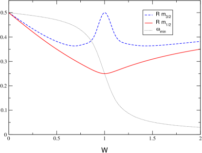
Figure 1: Plot of the minimum of the effective potential $\omega_{min}$ (dotted line) and the corresponding lightest KK mode mass for the gravitino (dashed line) and gaugino/hyperscalar (solid line) in units of $1/R$ for the case of only Standard Model gauge bosons propagating in the bulk: $N_{V}=12$, $N_{H}=0$.

As we have seen above, the presence of the brane induced supersymmetry breaking (4.2) modified the mass eigenvalues for gravitinos (4.2), gauginos (4.1) and hyperscalars (4.3). These in turn modify the one-loop effective potential computed in section 3 that results now in

$$V_{eff}(\omega) =\frac{3}{32\pi^{6}R^{4}}\,\left[{\rm Li}_{5}\left(e^{i2\pi\Delta_{3/2}(\omega,W)}\right)+{\rm h.c.}\right]$$

$$+ \frac{3(N_{V}-N_{H})}{64\pi^{6}R^{4}}\,\left[{\rm Li}_{5}\left(e^{i2\pi\Delta_{1/2}(\omega,W)}\right)+{\rm h.c.}\right]\,.$$ (4.21)

We expect that the brane effects modify continuously the location of the minimum of the effective potential away from its minima for $W=0$ at $\omega=0$ or $\omega=1/2$. We have studied numerically two extreme cases.

In Fig. 1 we have studied the case where only the gravitational and gauge sector are living in the bulk, while matter and Higgs fields are localized in the observable brane and thus do not participate in the one-loop effective potential. Of course the supersymmetric partners of localized matter will receive radiative masses from the bulk supersymmetry breaking [8]. In particular we have considered the supersymmetric Standard Model gauge sector in the bulk with $N_{V}=12$ and $N_{H}=0$. The result is shown in the plot where different quantities are shown vs. the parameter $W$. The dotted line is the value of the Scherk-Schwarz parameter at the minimum $\omega_{min}$. We can see that it is equal to $1/2$ for $W=0$ and goes smoothly to zero in the limit $W\to\infty$. Dashed and solid lines correspond to the values of the gravitino and gaugino/hyperscalar lightest KK modes.

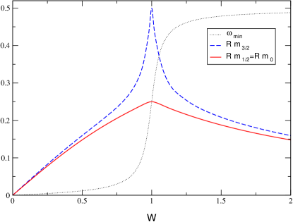
Figure 2: The same as in Fig. 1 for the case of all Standard Model fields propagating in the bulk: $N_{V}=12$, $N_{H}=49$.

Fig. 2 corresponds to the other extreme case where all gauge sector and matter (including two Higgs hypermultiplets) propagate in the bulk. For the case of the supersymmetric Standard Model $N_{V}=12$ and $N_{H}=3\times 15+4=49$. We can see that the minimum starts at $\omega_{min}=0$ at $W=0$ and goes to $\omega_{min}=1/2$ in the limit $W\to\infty$. In this limit the masses of lightest KK modes can be much smaller than $1/R$.

5 Conclusions

In this paper we have considered a supersymmetric five-dimensional brane-world scenario where the fifth dimension is compactified on $S^{1}/\mathbb{Z}_{2}$. In this set-up, the Scherk-Schwarz supersymmetry breaking can be interpreted as the Hosotani breaking of the $SU(2)_{R}$ local symmetry present in off-shell $N=2$ supergravity. We have shown that the Scherk-Schwarz supersymmetry breaking parameter is undertemined at the tree-level, but can acquire two discrete values after loop-corrections from supersymmetric bulk fields are introduced. In this way, supersymmetry may get broken radiatively through the Scherk-Schwarz mechanism. We have also computed the contribution to the soft supersymmetry breaking masses of bulk fields in the case in which a source of supersymmetry breaking appears localized on the hidden brane. In such a case, the Scherk-Schwarz supersymmetry breaking parameter is lifted away from the discrete values $0$ and $1/2$ and the spectrum of the KK modes of the bulk fields assumes a variety of possibilities depending upon the strength of supersymmetry breaking on the hidden brane.

References

- [1] I. Antoniadis, Phys. Lett. B246 (1990) 377; I. Antoniadis, C. Muñoz and M. Quirós, Nucl. Phys. B397 (1993) 515; I. Antoniadis and K. Benakli, Phys. Lett. B326 (1994) 69; I. Antoniadis, K. Benakli and M. Quirós, Phys. Lett. B331 (1994) 313; I. Antoniadis and M. Quirós, Phys. Lett. B392 (1997) 61.
- [2] P. Horava and E. Witten, Nucl. Phys. B460 (1996) 506 [hep-th/9510209]; P. Horava and E. Witten, Nucl. Phys. B475 (1996) 94 [hep-th/9603142]; P. Horava, Phys. Rev. D54 (1996) 7561 [hep-th/9608019].
- [3] I. Antoniadis and M. Quiros, Nucl. Phys. B505 (1997) 109 [hep-th/9705037]; I. Antoniadis and M. Quiros, Phys. Lett. B416 (1998) 327 [hep-th/9707208]; I. Antoniadis and M. Quiros, Nucl. Phys. Proc. Suppl. 62 (1998) 312 [hep-th/9709023].
- [4] H. P. Nilles, M. Olechowski and M. Yamaguchi, Phys. Lett. B415 (1997) 24 [hep-th/9707143]; H. P. Nilles, M. Olechowski and M. Yamaguchi, Nucl. Phys. B530, 43 (1998) [hep-th/9801030]; H. P. Nilles, hep-ph/0004064.
- [5] E. A. Mirabelli and M. E. Peskin, Phys. Rev. D58 (1998) 065002 [hep-th/9712214].
- [6] J. R. Ellis, Z. Lalak, S. Pokorski and W. Pokorski, Nucl. Phys. B540 (1999) 149 [hep-ph/9805377].
- [7] L. Randall and R. Sundrum, Nucl. Phys. B557 (1999) 79 [hep-th/9810155].
- [8] A. Pomarol and M. Quirós, Phys. Lett. B438 (1998) 255; I. Antoniadis, S. Dimopoulos, A. Pomarol and M. Quiros, Nucl. Phys. B544 (1999) 503 [hep-ph/9810410]; A. Delgado, A. Pomarol and M. Quiros, Phys. Rev. D60 (1999) 095008 [hep-ph/9812489].
- [9] D. E. Kaplan, G. D. Kribs and M. Schmaltz, Phys. Rev. D62 (2000) 035010 [hep-ph/9911293]; Z. Chacko, M. A. Luty, A. E. Nelson and E. Ponton, JHEP 0001 (2000) 003 [hep-ph/9911323].
- [10] T. Gherghetta and A. Pomarol, Nucl. Phys. B602 (2001) 3 [hep-ph/0012378].
- [11] G. von Gersdorff and M. Quiros, Phys. Rev. D65 (2002) 064016 [hep-th/0110132].
- [12] J. Scherk and J. H. Schwarz, Phys. Lett. B82 (1979) 60; J. Scherk and J. H. Schwarz, Nucl. Phys. B 153 (1979) 61; E. Cremmer, J. Scherk and J. H. Schwarz, Phys. Lett. B84 (1979) 83.
- [13] Y. Hosotani, Phys. Lett. B126 (1983) 309; Phys. Lett. B129 (1983) 193; Ann. Phys. 190 (1989) 233.
- [14] Z. Chacko and M.A. Luty, JHEP 0105 (2001) 067; T. Kobayashi and K. Yoshioka, Phys. Rev. Lett. 85 (2000) 5527; D. Martí and A. Pomarol, Phys. Rev. D64 (2001) 105025 [hep-th/0106256]; D.E. Kaplan and N. Weiner, hep-ph/0108001.
- [15] E. Cremmer, S. Ferrara, C. Kounnas and D. V. Nanopoulos, Phys. Lett. B133 (1983) 61; A. B. Lahanas and D. V. Nanopoulos, Phys. Rep. 145 (1987) 1.
- [16] J. A. Bagger, F. Feruglio and F. Zwirner, Phys. Rev. Lett. 88 (2002) 101601 [hep-th/0107128]; J. Bagger, F. Feruglio and F. Zwirner, JHEP 0202, 010 (2002) [hep-th/0108010].
- [17] T. Gherghetta and A. Riotto, Nucl. Phys. B623 (2002) 97 [hep-th/0110022].
- [18] E. Bergshoeff, R. Kallosh and A. Van Proeyen, JHEP 0010 (2000) 033 [hep-th/0007044].
- [19] R. Altendorfer, J. Bagger and D. Nemeschansky, Phys. Rev. D63 (2001) 125025 [hep-th/0003117].
- [20] T. Kugo and K. Ohashi, Prog. Theor. Phys. 104 (2000) 835 [hep-ph/0006231]; T. Kugo and K. Ohashi, Prog. Theor. Phys. 105 (2001) 323 [hep-ph/0010288]; T. Fujita, T. Kugo and K. Ohashi, hep-th/0106051; T. Kugo and K. Ohashi, hep-th/0203276.
- [21] M. Zucker, Nucl. Phys. B570 (2000) 267 [hep-th/9907082]; M. Zucker, JHEP 0008 (2000) 016 [hep-th/9909144]; M. Zucker, Phys. Rev. D64 (2001) 024024 [hep-th/0009083]; M. Zucker, “Off-Shell Supergravity in Five Dimensions and Supersymmetric Brane World Scenarios”, Ph. D. Thesis, Bonn University, BONN-IR-2000-10, August 2000.
- [22] M. F. Sohnius and P. C. West, Nucl. Phys. B216 (1983) 100.
- [23] R. Barbieri and S. Cecotti, Z. Phys. C17 (1983) 183; L. Baulieu, A. Georges and S. Ouvry, Nucl. Phys. B273 (1986) 366; M. K. Gaillard and V. Jain, Phys. Rev. D49 (1994) 1951 [hep-th/9308090].
- [24] E. Ponton and E. Poppitz, JHEP 0106 (2001) 019 [hep-ph/0105021].
- [25] A. Delgado and M. Quiros, Nucl. Phys. B607 (2001) 99 [hep-ph/0103058]; A. Delgado, G. von Gersdorff, P. John and M. Quiros, Phys. Lett. B517 (2001) 445 [hep-ph/0104112]; A. Delgado, G. V. Gersdorff and M. Quiros, Nucl. Phys. B613 (2001) 49 [hep-ph/0107233]; M. Quiros, J. Phys. G27 (2001) 2497.
- [26] R. Barbieri, L.J. Hall and Y. Nomura, Phys. Rev. D63 (2001) 105007; N. Arkani-Hamed, L.J. Hall, Y. Nomura, D. Smith and N. Weiner, Nucl. Phys. B605 (2001) 81; R. Barbieri, L. J. Hall and Y. Nomura, Nucl. Phys. B624 (2002) 63 [hep-th/0107004]; R. Barbieri, L. J. Hall and Y. Nomura, hep-ph/0110102.
- [27] D. M. Ghilencea, S. Groot Nibbelink and H. P. Nilles, Nucl. Phys. B619 (2001) 385 [hep-th/0108184].