hep-th/0204038

HUTP-02/A007

IFIC/02-13

Entropy-Area Relations in Field Theory

Lisa Randall¹, Verónica Sanz², Matthew D. Schwartz¹

¹ Jefferson Physical Laboratory

Harvard University, Cambridge, MA 02138

² Depto. de Física Teórica - IFIC, Centro Mixto

Universidad de Valencia-CSIC, Valencia, Spain

Abstract

We consider the contribution to the entropy from fields in the background of a curved time-independent metric. To account for the curvature of space, we postulate a position-dependent UV cutoff. We argue that a UV cutoff on energy naturally implies an IR cutoff on distance. With this procedure, we calculate the scalar contribution in a background anti-de Sitter space, the exterior of a black hole, and de Sitter space. In all cases, we find results that can be simply interpreted in terms of local energy and proper volume, yielding insight into the apparent reduced dimensionality of systems with gravity.

randall@physics.harvard.edu
Veronica.Sanz@ific.uv.es
matthew@feynman.princeton.edu

1 Introduction

The Bekenstein bound severely restricts the number of degrees of freedom in a gravitational system, bounding the entropy by $S<\frac{\mathcal{A}}{4\pi}M^{2}_{\mathrm{Pl}}$, where ${\mathcal{A}}$ is the area of the system. We would like to understand how to formulate field theory so that it manifestly reflects this lower number of degrees of freedom. The holographic principle tells how to associate a bulk region of space with a boundary region [1, 2]. In the case of AdS/CFT, the holographic principle is explicit because there exists an explicit duality between bulk and boundary theories [3]. Detailed tests of the conjecture have been performed [3, 4, 5] and new principles have been conjectured based on this correspondence [6]. Most systems will not exhibit this correspondence so simply; at the very least, the holographic dual to a bulk system would generally not be a local field theory, as with the linear dilaton theory for example [7]. Nonetheless, because AdS is so well explored, it makes sense to extrapolate lessons about the field theory in the bulk to see how far one can get by studying only the bulk theory, and not using anything about the existence of a holographic dual theory. This is motivated by the calculation done in Ref. [8, 9], where we derived a logarithmic running of the coupling in a five-dimensional calculation. We will use the regularization procedure employed there based on a cutoff on local energy to extract the essential physics that led to the appearance of reduced dimensionality of the field theory. Of course, for AdS space, the apparent reduced dimensionality might be simply the fact that volumes behave like areas, in the sense that integration over the direction perpendicular to the boundary only multiplies the area by a finite length, the AdS curvature, independent of the size of this dimension. In fact, this is in some sense true, and it is the purpose of this paper to generalize this simple intuition.

We are led to ask if we calculate the number of degrees of freedom in a curved space by generalizing this method, do we always get the right answer (or at least the correct dimensionality describing the number of degrees of freedom) by generalizing our regularization procedure. Clearly, because the cutoff is an artifact of not doing a full string theory calculation, we will not obtain precise answers with a trustworthy numerical coefficient. Nonetheless, it is of great interest that we will find that our answers scale in a way consistent with the Bekenstein formula; that is, the degrees of freedom fit on a space of one lower dimension. The main purpose of this paper is to demonstrate that by eliminating the region of space-time where energies are above a local cutoff scale, we can understand intuitively why and how a theory becomes holographic, in the sense of having degrees of freedom reflecting a space of reduced dimensionality. We will show this for global AdS, de Sitter space, and black holes.

Our procedure incorporates a cutoff on local energy that is reinterpreted as a cutoff on position for a given energy. Now we make a further assumption, that may be interpreted as a weak form of a UV/IR correspondence, and assume that there is an energy-dependent cutoff on the size of the space (IR) that reflects the energy cutoff (UV). That is, we assume that the region which does not permit the given value of energy does not exist and we quantize the system on this space of reduced size. This procedure will be explained more fully in Section 3 but clearly relies on an IR cutoff on the size of the space resulting from a UV cutoff on the local energy. The intuition for this assumption comes from the field theory AdS calculation of Ref. [9]. It reflects the fact that the space probed by the high energy modes is effectively smaller than the full space. The low mass modes have substantial amplitude only outside this region. Furthermore, the coupling changed in such a way to compensate for the larger mode spacing. Without detailed knowledge of the Kaluza-Klein spectrum, one cannot in general deduce the reduced dimensionality through the energy-dependent cutoff alone. Imposing the IR cutoff that reflects the local UV cutoff reproduces this structure of the modes.

This picture gives a simple origin for the reduction of degrees of freedom. By forcing local energy, $\sqrt{g^{tt}}E$, to be less than a cutoff $\Lambda$, the high energy modes will in general probe less of the space than the low energy modes. The spatial cutoff implements the correct counting. It reflects the physical fact that at high energy, there are regions of space that are inaccessible, so effectively the boundary depends on energy. This reduction of volume at high energy can have the same effect on thermodynamic quantities as confining the theory to a subspace, for example, the boundary. There is not necessarily a boundary theory; however, in certain cases (when a horizon exists for example), the physics is dominated by the degrees of freedom concentrated near this region.

Let us summarize the similarities and differences between our approach, and one that postulates the existence of a boundary theory. In both approaches, we find in certain known examples that the number of degrees of freedom scales with area, not volume. In our description, the degrees of freedom reside throughout the space, but might be peaked on the boundary. This should be contrasted with a boundary description where the degrees of freedom are fundamental degrees of freedom on a holographic screen. Our description only involves bulk degrees of freedom. We are not making any holographic correspondence. We simply note that the degrees of freedom reflect a theory of lower dimension, but we do not explicitly postulate such a theory. In the case of a black hole, our answer agrees with that suggested by a stretched horizon, although it would have some energy-dependent structure. Our procedure only works however in a curved background, since it does not incorporate any back-reaction, although the curved background does reflect strong gravitational effects. Clearly, this is not sufficient to derive area-law scaling for all systems. For example, we would have nothing to say with this procedure about flat space. That is because what we are trying to do is count only those states that can be properly treated with low-energy field theory. States for which the back-reaction would alter the gravitational background considerably should be excluded. We do not exclude all such states so we will not always see the Bekenstein bound. For example, although we eliminate all cutoff sized black-holes, we clearly do not eliminate all possible configurations that can form a black hole or have some other strong gravitational back-reaction. Therefore, even for the curved spaces we consider, we sometimes find certain parameter regimes that reflect the full dimensionality of the space. Although it is not the whole story, this simple procedure should provide some guidance in seeking a more comprehensive understanding of holography. It also suggests that even with the full bulk description of the space, there is not necessarily redundancy in the low-energy description, when the metric is properly accounted for. It should also be kept in mind that although we refer to a cutoff, we have in mind an ultimate non-field theoretic description of the theory that kicks in at that scale. The fact that our answers are cutoff dependent tells us how the entropy associated with the cutoff should scale with size of the system. Furthermore, because the local cutoff changes with the curvature of the space, it suggests that degrees of freedom that are best thought of as free fields in some contexts are strongly bound states in others. Our work tells only about the field theoretical contribution, which is in general less than the full counting.

One advantage of our method of counting, even when there exists a precise holographic description as in the AdS example, is that it indicates the wave function for states in the bulk theory associated with the holographic dual on the boundary. We will see this explicitly for global AdS where we can see why the Bekenstein bound applies to the bulk theory. Another advantage of our method is that regulates a theory to give finite entropy, even in the presence of a horizon in a way well motivated by the physics. ’t Hooft previously had introduced a brick wall cutoff to deal with this situation.

The organization of this paper is as follows. We will start by reviewing the regularization we applied to RS1. In Section 3, we present the techniques we use for counting degrees of freedom or calculating entropy. We show that the answer will be the answer one should expect, the integrated local energy over the proper volume, where only states consistent with the local cutoff are permitted. We also demonstrate the relation between our cutoff procedure and Pauli-Villars, which it closely resembles. Section 4 applies our methodology to global anti-de Sitter space, where we again see the reduced dimensionality from our simple procedure. Sections 5 and 6 explore de Sitter space and black hole space-times. We will see that the local UV cutoff obviates the need for ’t Hooft’s brick wall cutoff. In the following section, we speculate about the non-covariant nature of our result; in particular, why it might not entirely account for all states in time-dependent space-times. Finally, in section 8, we summarize our results and their implications.

2 Poincare Patch AdS

Before looking at the spatially-varying cutoff in general space-times, we explain how it applies in the two brane RS1 model [10]. This model is fairly well understood, phenomenologically viable, and believed to be holographic [11, 12]. The background geometry is the Poincare patch of 5D anti-de Sitter space with metric:

$$ds^{2}=\frac{1}{(kz)^{2}}(-dt^{2}+d{\mathbf{x}}^{2}+dz^{2})$$ (1)

The bulk cosmological constant is -$3k^{2}$ which we assume to have a large magnitude, of order the Planck scale. In RS, the AdS horizon is cutoff by a Planck brane at $z_{0}=\frac{1}{k}$ and a TeV brane at $z_{1}=\frac{1}{T}$, where $T$ is a mass scale of order TeV. It is clear from (1) that the induced geometry at any fixed $z$ is flat. It is also not hard to show that at low energies the bounded fifth dimension can be integrated out to get an effective theory which is flat as well.

Let’s suppose we have a scalar field which is free to propagate in the bulk. A simple hypothesis is that the total number of degrees of freedom of such a field is given roughly by the volume of the space normalized with some UV cutoff $\Lambda$ [2]:

$$g(\Lambda)\approx\Lambda^{4}\int\sqrt{-G}d^{3}xdz\approx\Lambda^{4}L^{3}\int^{1/T}_{1/k}\frac{1}{(kz)^{4}}dz\approx\Lambda^{3}L^{3}\Lambda(\frac{k^{4}-T^{4}}{k^{5}})\approx\Lambda^{3}L^{3}\frac{\Lambda}{k}$$ (2)

For large $k\approx\Lambda$, this looks like a 4D system.

Now, suppose we tried to count the degrees of freedom by adding up the Kaluza-Klein (KK) modes of the bulk field. The massless field in 5D can be decomposed into a set of 4D modes with masses given by roughly $m_{n}=jT$ for integer $j$. Then each mode satisfies:

$$E^{2}=p^{2}+m_{j}^{2}$$ (3)

where $p$ is the 3-momentum. The number of states with energy less than $E$, $g(E)$, is given by:

$$g(E)=\int_{0}^{E/T}djL^{3}\int_{0}^{\sqrt{E^{2}-(jT)^{2}}}p^{2}dp\sim E^{3}L^{3}\frac{E}{T}$$ (4)

So $g(\Lambda)=\Lambda^{3}L^{3}\frac{\Lambda}{T}$. This superficially has the same form as (2), but we expect $\Lambda\approx k\gg T$. Since $\frac{1}{T}$ is the size of the fifth dimension, this wrongly implemented Kaluza Klein picture makes it seem like there are 5D degrees of freedom.

These two results are different because the volume calculation is scaling the cutoff with position, while the KK calculation, as presented above, is not. Indeed, the contribution to the volume at a position $z$ is not $\Lambda^{4}L^{3}dz$ but $\frac{\Lambda^{4}L^{3}}{k^{5}z^{5}}dz$.

In [8, 9], a position-dependent regulator was introduced. By calculating Feynman diagrams in 5D, we showed that gauge couplings in the 5D bulk run logarithmically, that is as in 4D, and that perturbative unification is feasible at a high scale in $\mathrm{AdS}_{5}\;$. What we want to emphasize here is not the details of the calculation, but why the result is to be expected with a generally covariant cutoff in place.

When we did a field theory calculation in AdS₅, we did not use explicit KK modes, but did our calculation in the five-dimensional space with a mixed position space/momentum space formulation, integrating over $p_{\mu}$ and $z$. We applied a cutoff on momentum $p$ that varied with position in accordance with the warp factor, that is $p(z)<\Lambda$ or equivalently, $p<\Lambda(z)$ where

$$\Lambda(z)=\frac{1}{kz}\Lambda$$ (5)

This is the spatially-varying cutoff on energy; the UV cutoff on $p$ depends on position (see Figure 1). The highest cutoff is on the Planck brane, where $\Lambda(\frac{1}{k})=\Lambda$. On the TeV brane, $p$ can only go up to $\Lambda\frac{T}{k}\ll\Lambda$. Because $p<$ $\frac{1}{kz}\Lambda$ is the same constraint as $z<\frac{\Lambda}{kp}$ and $p<\Lambda$, the position-dependent cutoff is equivalent to a usual cutoff on 4D momenta and an energy-dependent limit on $z.$ By taking this constraint on $z$ as the new boundary of the system, one can readily see that the number of states is drastically reduced and agrees with the holographic expectation.

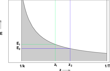
Figure 1: In the RS1 model, an IR boundary at $z=1/T$ is effectively replaced for energies $E>\frac{\Lambda}{k}T$. The new boundary, shown for two modes with energies $E_{1}$ and $E_{2}$, is at $z_{1(2)}=\frac{\Lambda}{k}\frac{1}{E_{1(2)}}$. The area of the ($E,z$) plane satisfying $E<\Lambda(z)$ is shaded.

We emphasize that there are two aspects to this procedure. First, there is a spatial-cutoff for a given energy. Second there is a re-quantization reflecting this spatial cutoff for each energy. For this RS1 Poincare patch example, we get the right counting even without moving the boundary. However, in general, we have to move the boundary explicitly for each energy to reproduce what we expect from the more detailed mode analysis. This was the actual procedure used in Ref. [8, 9].

Not only does the above calculation demonstrate 4D behavior, it shows that there is an intermediate regime that appears to be 5D [11]. The cutoff is position dependent only for $p>\frac{\Lambda}{k}T$. At lower energies, the cutoff is fixed at $z=\frac{1}{T}$. In this regime, the constraint on $z$ would have implied a brane deeper in the IR than the TeV brane, so it is irrelevant. At very low energies $p<T$, no KK modes are excited and the theory is 4-dimensional: $g(E)=(EL)^{3}$. If $T<p<\frac{\Lambda}{k}T$ then $E^{2}=\mathbf{p}^{2}+j^{2}T^{2}$. Therefore in this regime, one obtains the usual 5D dispersion relation, and $g(E)=\frac{E}{T}(EL)^{3}$. When $E/T>\Lambda/k$ we are in the holographic regime. In summary, the theory appears to be 4D for $E<T$, 5D for $\frac{\Lambda}{k}T>E>T$ and 4D for $E>\frac{\Lambda}{k}T$.

3 Other Geometries

Now that we have seen how the spatially-varying cutoff leads to holographic thermodynamics and $\beta$-functions in the RS1 model, we generalize to other geometries. For time-independent metrics, the killing vector $\partial_{t}$ allows us to assign an energy $E$ to any state. As we justified above, this energy should never be greater than the locally measured cutoff $\Lambda(r)=\sqrt{g_{tt}(r)}\Lambda$. The state with energy $E$ should only probe the region where $\Lambda(r)\geqslant E$. So the boundary $r_{E}$ at an energy $E$ is determined by:

$$E=\sqrt{g_{tt}(r_{E})}\Lambda$$ (6)

The $E$-dependent cutoff on $r$ will determine the quantization of momentum in the $r$ direction, and hence the quantization of $E$ itself. In some cases, one can derive details about the spectrum; however, even without the precise spectrum, we can evaluate approximately the density of states.

In the examples below, we focus on metrics which take the form

$$\mathrm{ds}^{2}\;=-V(r)\mathrm{d}t^{2}\;+\frac{1}{V(r)}\mathrm{d}r^{2}\;+r^{2}d\Omega^{2}$$ (7)

Some examples are global anti-de Sitter space $V(r)=1+k^{2}r^{2}$, static de Sitter $V(r)=1-k^{2}r^{2}$, the exterior of Reissner-Nordstrom black holes $V(r)=1-\frac{2m}{r}+\frac{q^{2}}{r^{2}}$. This is an interesting class of metrics in that they are examples in which area laws are known to apply. Furthermore, as we will discuss, they all manifest UV/IR correspondence.

Consider the covariant Klein-Gordon equation:

$$\frac{1}{\sqrt{g}}\partial_{\mu}(\sqrt{g}g^{\mu\nu}\partial_{\nu}\phi)=M^{2}\phi$$ (8)

We first consider states in the 4D system. In the background (7), and with the ansatz $\phi=\varphi(r)Y_{\mathrm{lm}\;}(\theta,\phi)e^{iEt}$, (8) becomes:

$$\frac{E^{2}}{V(r)}\varphi+\frac{1}{r^{2}}\partial_{r}(r^{2}V(r)\partial_{r}\varphi)-\frac{l(l+1)}{r^{2}}\varphi-M^{2}\varphi=0$$ (9)

This is just a 1D quantum mechanics problem. The spatially-varying cutoff would enter through the boundary conditions which will depend on $E$.

With the exact spectrum, one can evaluate the density of states. Even without the exact spectrum, one can often use the semi-classical (WKB) approximation [13]. Alternatively, one can evaluate the density of states based on the local energy and proper distance in accordance with the metric. We will see that both these last two methods give yield the same formula for calculating the density of states.

WKB applies when the phase of the wavefunction changes much faster than the amplitude. We can then write $\varphi=\sqrt{\rho}e^{iS(r)}$ and assume that $k(r)=S^{\prime}(r)$ is large. This allows us to solve (9) implicitly (for $M=0$):

$$k(r,E,l)=\frac{1}{V(r)}\sqrt{E^{2}-\frac{V(r)}{r^{2}}l(l+1)}$$ (10)

The number of oscillations of the phase of $\varphi$ over the whole space is the number of nodes of the approximate wavefunction. This is roughly the number of modes with energy less than $E$. Indeed, as $E$ is lowered to zero, each of these nodes should disappear; whenever a node hits the endpoint, there is another state. Thus the number of states with energy less than $E$ is given by

$$g(E)=\int\mathrm{dr}\;\int k(r,E,l)(2l+1)dl=\int\frac{\mathrm{dr}\;}{V(r)}\int(2l+1)dl\sqrt{E^{2}-\frac{V(r)}{r^{2}}l(l+1)}$$ (11)

The integral over $l$ is for values of $l$ which keep $k$ positive, that is $l(l+1)<\frac{r^{2}E^{2}}{V(r)}$. This gives:

$$g(E)=\frac{2}{3}E^{3}\int\frac{r^{2}}{V(r)^{2}}dr$$ (12)

Note that $g(E)$ already seems to have 4D $E$ dependence. So, unless the $r$ integral depends on $E$, we will have 4D thermodynamics. In our regularization, we limit $r$ by $E<\sqrt{V(r_{E})}\Lambda$. This will add $E$-dependence to the $r$ integral. For example, if $V(r_{0})=0$ at a horizon, then the integrand will have a pole. The only modes that can probe up to the horizon have $E=0$, so the pole is an $E=0$ pole and must change the $E$ dependence of the density of states for low energy. We will show this explicitly in later sections.

In fact, (12) is precisely the answer we expect in four dimensions once the metric is properly accounted for. That is, for an $n$-dimensional space, we expect the number of degrees of freedom to be

$$g(E) \approx \int^{r_{E}}\left(\sqrt{g^{tt}}E\right)^{n-1}r^{n-2}\sqrt{g_{rr}}dr$$

$$\approx \int{E^{n-1}\over V(r)^{\frac{n}{2}}}r^{2}dr$$

One can partially understand the relation between the position-dependent cutoff and a Pauli-Villars regulator by examining the form of the equation of motion. Since we are concerned with time-independent metrics, we write $\phi=\varphi(x)e^{iEt}$ and the Klein-Gordon equation (8) becomes

$$g^{tt}(x)E^{2}\varphi+\frac{1}{\sqrt{g}}\partial_{i}(\sqrt{g}g^{ij}\partial_{j}\varphi)=M^{2}\varphi$$ (14)

The Green’s function for a quantum field and for its PV regulator at an energy $E$ will satisfy (14). The PV field has negative norm so its propagator will cancel the regulated field wherever the PV mass has a negligible effect on the propagator. In particular, there will be a thorough cancellation for all values of $x$ which satisfy $g^{tt}(x)E^{2}\gg M_{\mathrm{PV}}^{2}$. This is equivalent to equation (6) for $\Lambda=M_{\mathrm{PV}\;}$.

As an example of the equivalence between our regularization procedure and Pauli-Villars, we look again at the RS1 model. PV was used in this scenario in [14]. The propagators for massless and massive fields were derived in [8] and involve Bessel functions such as $\mathcal{J}_{\nu}(pz)$ where $\nu=\sqrt{1+M^{2}/k^{2}}$ and $p$ is the momentum. These functions have the nice property that $\mathcal{J}_{\nu}(x)$ is independent of $\nu$ (up to a phase) for $x\gg\nu$. Thus, the propagator for a field and its PV regulator will cancel if $z>\frac{\nu}{p}\approx\frac{M}{kp}$. This is exactly the condition we use when applying the position-dependent cutoff.

Once we have $g(E)$, we can generate all the important thermodynamic quantities. The free energy is:

$$F=-\frac{1}{\pi}\int\frac{g(E)}{e^{\beta E}-1}dE$$ (15)

Which gives $U=\frac{\partial}{\partial\beta}(\beta F)$ and $S=\beta(U-F)$. For our examples, the scaling of $g(E)$ with $E$ will be the same as the scaling of $S(T)$ with $T$.

4 Global AdS

In [4, 16], the thermodynamics of global AdS was considered. Witten found that at a temperature of order $k$ (the AdS curvature scale), there is a transition from pure AdS to AdS-Schwarzschild, above which both the bulk and boundary theory reflect the number of degrees of freedom of a four-dimensional theory in that the entropy scales as $T^{4}$. We now show that our counting of states agrees with the above transition between that of a low-energy theory and one for which it reflects the full dimensionality (our estimate of states will not reflect the gap). More precise agreement would require choosing $\Lambda$ and the number of fields in accordance with the holographic correspondence (see below).

The AdS potential is $V(r)=1+k^{2}r^{2}$. To apply our procedure, we introduce a boundary regulator brane at a position $r=R$. Also, for simplicity, we consider $AdS_{5}$ rather than $AdS_{5}\times S^{5}$. As explained in the previous section, we expect the number of states is approximately (note that now we are in 5D):

$$g(E)\sim E^{4}\int_{r_{E}}^{R}{r^{3}dr\over V(r)^{5/2}}\sim E^{4}\int_{r_{E}}^{R}{r^{3}dr\over k^{5}r^{5}}$$ (16)

where the last approximation is valid for $r\gg 1/k$. In this equation, $r_{E}$ is chosen in accordance with a spatially varying cutoff as described in Section 3, $\Lambda(r)=\sqrt{1+k^{2}r^{2}}\Lambda$. Setting $\Lambda(r_{E})=E$ leads to

$$r_{E}=\frac{1}{k}\sqrt{\frac{E^{2}}{\Lambda^{2}}-1}\sim\frac{E}{k\Lambda}$$ (17)

The number of states is now readily evaluated to find

$$g(E)\sim\left({E\over k}\right)^{4}\left({\Lambda\over E}\right)\sim\left({E\over k}\right)^{3}{\Lambda\over k}$$ (18)

This shows the dependence on energy of a four-dimensional theory when $E$ is sufficiently large, as anticipated. Notice the confinement of the high energy modes to the region near the boundary yields the factor of $1/E$ that converts the behavior from five to four-dimensional.

For low energies, $E<\Lambda$, the answer will not be that of a lower-dimensional theory. That is to be expected, since for these energies, one is probing distance scales less than $1/k$, for which the theory should resemble flat space. This follows when applying our regulator, since for energies less than $\Lambda$, the entire space, down to arbitrarily small $r$, can support the state. Actually, a more careful analysis with the precise modes would reflect the band gap that would limit this 5D scaling behavior to energies between $k$ and $\Lambda$. In summary, the theory appears to have 5-dimensional counting of states for $k<E<\Lambda$ and appears 4-dimensional for $E>\Lambda$. Notice that this behavior closely resembles what we found for the Poincare patch calculation, which had the fewest modes at low energies, then had a five-dimensional regime, then evolved to the holographic four-dimensional regime.

We can ask what we learn from this method that we did not already know by using the precise holographic dual [15]. The answer is that we have a guide to the precise nature of the correspondence, since we can see what states exist in the bulk dual theory. For example, in the state counting done by Susskind and Witten, the Bekenstein bound was assumed for the bulk. But if we use the additional information of precisely what the cutoff should be as determined by the duality, we can see this counting of bulk states explicitly. To see this, we use the coordinate parameterization of AdS space assumed in that paper, where $V(r)=1/(1-(kr)^{2})^{2}$ and $k$ sets the AdS curvature scale. Then with a regulator brane a distance $\delta$ from the boundary, the 4D theory would have a cutoff on distance $\delta$ so that the cutoff on proper distance is $1/k$. Then the volume of the AdS₅ is $(1/k)\times{\mathcal{A}}\times k^{4}$, where ${\mathcal{A}}$ is the 3D area and we have used the cutoff $k$ provided by the dual holographic theory, which we know for this example. From this, we almost have a result well within the Bekenstein bound. But this was for a single field in the bulk. We expect that the description of the holographic dual would require $N^{2}$ such fields so that the total maximum entropy would be $N^{2}{\mathcal{A}}k^{3}$, where $N$ is a parameter from the dual theory.

We can also obtain the answer for the density of states through studying directly the eigenvalue spectrum. For simplicity, we show a 4D AdS example, rather than the 5D example we just looked at. When $E>\Lambda$ we restrict $r$ by $r_{E}<r<R$. Let us take the limit $Rk\gg 1$ and $E\gg\Lambda$. If we change variables to $\rho=\frac{r_{E}}{r}$ and define $\varphi=\rho\chi(\rho)$ then in this limit, (9) simplifies to an analog quantum mechanics problem:

$$-\partial^{2}_{\rho}\chi+\frac{2}{\rho^{2}}\chi-\frac{\Lambda^{2}}{k^{2}}(1-\frac{l(l+1)k^{2}}{E^{2}})\chi=0$$ (19)

Note that we have absorbed the spatially-varying cutoff into the normalization of $\rho$ so this equation has boundary conditions at fixed $\rho$. The solutions are Bessel functions (in fact, they are the same Bessel functions as in the 4D Poincare patch case). The eigenvalues for each $l$ are integers $j_{l}$ related to the energy and other parameters as:

$$j_{l}^{2}=\frac{\Lambda^{2}}{k^{2}}(1-\frac{l(l+1)k^{2}}{E^{2}})$$ (20)

In other words:

$$E^{2}=\frac{l(l+1)k^{2}}{1-(\frac{nk}{\Lambda})^{2}}$$ (21)

Therefore the number of modes at each $l$ is bounded by $n<\frac{\Lambda}{k}$. The total number of modes less than $E$ is $g(E)\sim\frac{\Lambda}{k}(\frac{E}{k})^{2}$. This density of states is 3D which is holographic to the 4D background.

Notice that the energy scale here is different from the Poincare Patch example. With the regulator brane there is the potential for a phenomenologically viable 4D theory of gravity if we choose the energy cutoff to be of order $M_{Pl}$, which is related to the 5D Planck scale $M$ by $M_{Pl}=(\frac{M}{k})^{3/2}k^{2}R$. For large $R$ this is a much higher cutoff than the natural expectation $\Lambda\approx M$ which we have used.

5 Black Hole Thermodynamics

In this section, we consider the contribution to the entropy from a scalar field in the exterior of a black hole [13, 18]. Although this is not the fundamental contribution to a black hole’s entropy, it can give us information about the scaling with cutoff and dimension of this fundamental contribution which should have the same dimension-dependence.

Black holes and de Sitter space (see next section) differ from the AdS examples we just studied in that states are concentrated not on a boundary where $g_{tt}$ is largest but on a horizon, where it is smallest. It might seem surprising that our method of counting states would yield a concentration of states on the horizon, since, as we have emphasized, the number of states is reduced by restricting states to a region where they are consistent with the local cutoff. By this reasoning, we would expect high energy states to be concentrated away from the horizon so that the entropy would also be concentrated there.

However, state counting proceeds differently in the black hole and de Sitter space examples, because we assume that there is a fixed temperature, $T$, as measured at infinity (or the origin for de Sitter space). Therefore, in general, the energy stays well below the local cutoff. In fact, energy at a given position $r$ will be chiefly of order $T/\sqrt{V(r)}$, where $V(r)$, given in Section 3, goes to zero near the horizon. This means that for a fixed $T$, the highest energy region is where $V(r)$ is smallest, the opposite of what happens if we allow all energies up to the cutoff at all $r$. In fact, energies only achieve the local cutoff near the horizon. With no cutoff on energy, they would diverge as one approaches the horizon. We assume a cutoff on energy $\Lambda$ which we expect to be of order $M_{Pl}$. This in turn implies a cutoff on position; states cannot get too close to the horizon unless they have arbitrarily low energy (as measured at infinity).

For a black hole, $V(r)=1-\frac{r_{S}}{r}$, where $r_{S}=\frac{2m}{M^{2}_{Pl}}$ is the location of the horizon and $m$ is the mass of the hole. Generalizations to rotating or charged black holes are straightforward. The unregulated density of states diverges at $r=r_{S}$ because $V(r_{S})=0$. Following the prescription of Section 3, we define the cutoff to be $\Lambda$ at $r=\infty$. Then the closest a state of energy $E$ can get to the horizon is determined by $\sqrt{V(r_{E})}\Lambda=E$. So,

$$r_{E}=r_{S}\frac{\Lambda^{2}}{\Lambda^{2}-E^{2}}$$ (22)

The solution to the analog quantum mechanics problem has been extensively studied without energy-dependent boundary conditions (see, for example, [17]). For our purposes, it will be sufficient to estimate the density of states using Section 3.

In order to regulate the IR divergence from the asymptotic Minkowski space, we restrict space to a box of size $L$. Then the number of states calculated with (22) and (12) is

$$g(E)\approx\frac{2}{3}r_{S}^{3}\Lambda^{2}E+\frac{2}{9}L^{3}E^{3}+\mathcal{O}(\frac{r_{S}}{L})+\cdots$$ (23)

The $L^{3}E^{3}$ term is just what we expect from flat space. The other term is the leading contribution associated with the black hole. The cutoff dependence comes from a factor of $r_{E}-r_{S}$, which scales as $(E/\Lambda)^{2}$. The entropy which follows from the $L$-independent part of this $g(E)$ scales with temperature as:

$$S(T)\propto r^{3}_{S}T\Lambda^{2}+\cdots$$ (24)

Substituting in the Hawking temperature, we see the black hole contribution scales with the horizon area.

If we used the Reissner Nordstrom black hole potential, $V(r)=(1-\frac{r_{+}}{r})(1-\frac{r_{-}}{r})$ (24) would have been replaced by

$$S(T)\propto\frac{r^{4}_{+}}{r_{+}-r_{-}}T\Lambda^{2}+\cdots$$ (25)

Note that the RN temperature is $T_{RN}=\frac{r_{+}-r_{-}}{4\pi r_{+}^{2}}$ which makes $S(T_{RN})\propto{\mathcal{A}}\Lambda^{2}$ where ${\mathcal{A}}=4\pi r_{+}^{2}$ is the area of the horizon.

This computation follows closely that performed by ’t Hooft in Ref. [13], in which he assumed a sharp cutoff at a coordinate $h$ corresponding to a proper distance of order $1/M_{Pl}$. In our approach, states are kept away from the horizon due to a cutoff on energy, so that a state with finite energy cannot reach the horizon. So the minimum distance of a state from the horizon depends on energy. Because the energy at a position $r$ is of order $T/\sqrt{V(r)}$, the contribution is heavily concentrated in the high proper energy states that are closest to the horizon. In fact, it is easy to see that the proper distance of these states from the horizon is of order $1/M_{Pl}$, as in ’t Hooft’s calculation.

Our calculation is even closer in spirit to that of Demers, Lafrance, and Myers [18]. They also calculated the entropy contributed from a scalar field external to a black hole. Their calculation employed a Pauli-Villars regulator, which we have already shown closely matches our regulator. They furthermore verified the suggestion of Susskind and Uglum Ref. [19] by demonstrating the renormalization of the entropy was consistent. In flat space, Newton’s constant gets renormalized as:

$$\frac{1}{G_{N}}\rightarrow\frac{1}{G_{N}}+\frac{B}{12\pi}$$ (26)

where $B$ is some quadratically divergent function of the five PV masses. Then they use the same PV fields to regulate the divergence of the entropy outside a black hole. The entropy they get, using the same WKB technique, is $S(T)\propto\frac{r_{+}^{4}}{r_{+}-r_{-}}TB$. Note the similarity to (25). They then interpret this as a renormalization of the black hole entropy:

$$S_{\mathrm{BH}\;}=\frac{\mathcal{A}}{4G_{N}}\rightarrow\frac{\mathcal{A}}{4}(\frac{1}{G_{N}}+\frac{B}{12\pi})$$ (27)

The important point is that this is the same quadratically divergent function $B$ as in (26).

It is also straightforward to work out the logarithmic corrections. We obtain a term in (25) proportional to $\frac{r_{+}^{4}}{r_{+}-r_{-}}T^{3}\log(\Lambda)$. This piece corresponds to the divergent contribution $T^{3}\log(M)$ in [18]. The scale for the logarithm is naturally set by the black hole temperature $T_{RN}$. We can interpret this logarithm as a constant contribution related to higher curvature terms on the gravitational action [18, 20], being absorbed in the renormalization of higher dimension operators in the gravity action.

This result would be especially appealing in a theory of induced gravity. There the fact that both $G_{N}$ and the entropy receive the same contribution which grows with the number of degrees of freedom would guarantee there is no problem with a large number of species. We also observe that in this case, one might be able to understand the small value of $G_{N}$ as a result of a large number of species.

Clearly, there is a contribution to black hole entropy not associated with an external field. Very likely, this contribution is associated with whatever regulates the quantum field theory at energies of order the cutoff $\Lambda$. From this perspective, it is not surprising that there exists a string theory example where the full entropy is reproduced [21]. Furthermore, this shows on quite general grounds that whatever the cutoff physics contribution is, it should scale quadratically with associated mass scale and be proportional to area, in order to absorb the cutoff dependence of our field theory result, rendering it scheme-independent.

Finally, it is of interest to reflect on the form of the result. We found that for a black hole at the Hawking temperature, the entropy had a term that scaled with the volume of the space and an additional term that is attributed to the black hole that scales as $S\propto\Lambda^{2}R^{2}$, where $\Lambda$ is the cutoff and $R$ is the Schwarzschild radius. In fact, the answer really scales as $E^{3}R^{3}(\Lambda/E)^{2}$, and when averaging over the thermal ensemble, $E$ gets replaced by $T$, which is taken to be the Hawking temperature. Clearly, the first factor is what one would expect for the volume inside the black hole horizon. From this perspective, we see that the number of degrees of freedom is in fact far greater than the expected number for a system at such low temperature. How are we to understand this result?

Let us consider the value of $r_{H}-r_{S}$, where $r_{H}$ is the minimum $r$ permitted by our regularization procedure for a mode of energy $T_{H}=1/R$. One finds $(r_{H}/r_{S}-1)=(T_{H}/\Lambda)^{2}$. This corresponds to the proper distance from the horizon equal to $1/\Lambda$, what one would expect to be the minimum distance permitted in a system with cutoff $\Lambda$. Notice that in this sense, our regularization is naturally leading to the notion of a stretched horizon [22]. The degrees of freedom are concentrated at and around the coordinate $r_{H}$. Of course, we are not making any further claims; we do not consider a membrane as a physical object. We are simply making the observation that with our cutoff procedure, the degrees of freedom naturally tend to congregate at this position.

Furthermore, we understand the enhancement of the number of degrees of freedom over that which is expected. We see that the proper energy at $r_{H}$ is actually $\Lambda$, not the much smaller $T_{H}$. This is not surprising as this is how $r_{H}$ was chosen. But we see that the large number of degrees of freedom is due to the much higher proper energy of the modes at $r_{H}$. In fact, we can eyeball the result by taking the quantity $E_{p}^{3}\delta r_{p}^{3}$, where $E_{p}=E/(\sqrt{r_{h}/r_{S}-1})$ is the proper energy and $\delta r_{p}=(r_{h}-r_{S})/(\sqrt{r_{h}/r_{S}-1})$. Of course, this is restating the interpretation given in general in Section 3.

6 Static Patch of de Sitter Space

The final example we consider is de Sitter space, for which the entropy is bounded and is expected to take the form $S_{\mathrm{BH}\;}\propto M^{2}_{\mathrm{Pl}\;}R^{2}.$ We can compute the quantum corrections to this formula, as above for the exterior of the black hole.

The de Sitter function is $V(r)=1-\frac{r^{2}}{R^{2}}$ with $0<r<R$. Since $V(r)$ decreases as we approach the boundary, the cutoff $\Lambda(r)=\sqrt{V(r)}\Lambda$ has its maximum at $r=0$. Setting $\Lambda(r_{E})=E$ gives $r_{E}=R\sqrt{1-\frac{E^{2}}{\Lambda^{2}}}$. The state counting of Section 3 gives:

$$g(E)=\frac{R^{3}}{3}\Lambda^{2}E\left(\sqrt{1-\frac{E^{2}}{\Lambda^{2}}}-\frac{E^{2}}{\Lambda^{2}}\mathrm{Tanh}^{-1}\;(\sqrt{1-\frac{E^{2}}{\Lambda^{2}}})\right)$$ (28)

This function looks like a hump peaked around $E\approx 0.46\Lambda$.

However, we are only interested in counting the states at low energy, since we assume the space is at the de Sitter temperature. Then,

$$g(E)=\frac{R^{3}}{3}\Lambda^{2}E+\cdots$$ (29)

The linear energy-dependence arose because the distance to the horizon of a state of energy $E$ scales as $(E/\Lambda)^{2}$, as in the black hole example, which has the same near horizon structure.

The entropy is

$$S\propto R^{3}\Lambda^{2}T$$ (30)

Evaluated at the de Sitter temperature $T=T_{\mathrm{dS}\;}\approx\frac{1}{R}$ this says that $S_{\mathrm{dS}\;}=R^{2}\Lambda^{2}$. We expect that as with the black hole entropy, there is an associated renormalization of Newton’s constant. There are also logarithmically divergent pieces which correspond to the renormalization of higher dimension operators, as with black holes.

Notice that as with the black hole case, this is a much larger number of states than would be expected in a box of radius $R$ in flat space at temperature $T$, which scales like $R^{3}T^{3}$. This enhancement arises in a similar manner to the enhancement of states for a black hole at low temperature that we already discussed. Notice also that the entropy we calculated is not obviously a restriction on the number of states, but just corresponds to the number of states at the de Sitter temperature. The fundamental description of the system in principle involves many more states, most of which do not participate.

7 Coordinate Dependence

In the previous sections, we illustrated the utility of the spatially varying cutoff in reproducing qualitatively the known results for the entropy in several different geometries. The AdS case is well understood, although there are still puzzling features such as the explicit implementation of the UV/IR correspondence [6]. The black hole case is less well understood and exhibits some interesting features that we discuss in more detail in this section.

Although we understood the form of our answer in terms of local energy and proper volume, there is an obvious issue that we have so far skirted which is the coordinate dependence of our result. Some of the coordinate dependence of course comes from the non-covariant nature of the way we implemented our cutoff. A more careful analysis would use Pauli-Villars, which we have shown our method closely approximates. We use our procedure because the counting is very simple.

However, more worrisome for the black hole example is that one can choose coordinates that are completely smooth at the horizon. Where would the cutoff dependence of black-hole entropy then arise? We will necessarily be speculative in our considerations in this section. However, we find it suggestive that our results overlap with proposals that have already been made.

The key criterion that distinguishes the metrics in which we do our calculations from those we have avoided is that the ones we use are time-independent. For metrics that are strongly time-dependent, our cutoff procedure simply does not apply and we do not know how to do a calculation of the sort we have outlined since we cannot count energy eigenstates as we have been doing. We will next explain what goes wrong in several alternative parameterizations of the black hole metric. We will also argue by following the details of the coordinate transformation that there might exist long wavelength modes or nonlocal correlations that are not accounted for in low-energy field theory and which are sensitive to the cutoff physics. This would be a correction to low-energy field theory when counting degrees of freedom. However, these modes should be very low energy and long wavelength, and therefore irrelevant at a practical level, in which field theory should still apply.

7.1 Kruskal Coordinates

To get coordinates which are smooth at the horizon, we first transform from Schwarzschild ($r$,$t$) to advanced and retarded Eddington-Finkelstein coordinates:

$$U = t+r-r_{s}\log|r/r_{s}-1|$$ (31)

$$V = t-r-r_{s}\log|r/r_{s}-1|$$ (32)

The metric in these coordinates is still not well-behaved at the horizon, but it remains Minkowski for large $r$. In Kruskal coordinates: $x=e^{U}$, $y=e^{V}$, the metric is:

$$ds^{2}={32M^{3}\over r}e^{-r/r_{S}}dxdy+r^{2}d\Omega^{2}$$ (33)

There is no longer a singularity at the horizon. However for large $r$, the metric looks like $ds^{2}=\frac{dxdy}{xy}+r^{2}d\Omega^{2}$. This is not Minkowski and one has to worry about physics far away from the horizon. As an example of how we must be careful using our physical intuition in these coordinates, consider a mode near the horizon. It has very small energy measured at infinity, and we define $\epsilon=\frac{E}{\Lambda}$. The distance to the horizon this mode can probe is $r_{min}=r_{S}+\epsilon^{2}r_{S}$. To measure this mode, one would need an amount of Schwarzschild time approximately equal to $\Delta t=\frac{1}{E}=\frac{1}{\epsilon\Lambda}$. In Eddington-Finkelstein coordinates this means that $\Delta U\approx\Delta V\approx\frac{1}{\epsilon}$. While this is large, the space-like combination $U-V$ is still small. However, in Kruskal coordinates, $\Delta x\approx\Delta y\approx\epsilon e^{\frac{1}{\epsilon\Lambda}}$. Now the distance measured with respect to the space-like combination $x-y$ is exponentially large. Since the space is flat near the horizon, this corresponds to an exponentially large proper distance as well.

Tidal effects make any given region grow with $t$ in terms of $x$ and $y$ coordinates. We see that taking the minimum time that would be necessary to probe low energy states near the horizon, the near-horizon region is transformed into a huge region. We would expect a large number of low-energy states associated with this patch. These are not anticipated in the field theory associated with the patch that corresponded to the near-horizon region.

It is of interest to consider the possibility of such low-energy states. Because they are very large and low-energy, they would not affect any local physics so they are not precluded by the success of low-energy field theory. In fact, they are not necessarily states but could be correlations in existing states that store information. In this sense, they would be similar to the “precursors” suggested in Ref. [6, 23]. Also, because these states are sensitive to the cutoff of the theory, as has already been emphasized, we see this would implement a UV/IR connection [15, 24]. Finally, it is perhaps not unexpected that such large nonlocal states should exist in this new coordinate system, since the existence of an event horizon summarizes physics that is extended in time. In the new coordinates, where time and space are mixed, there might be new extended states.

Although we did the exercise for Kruskal coordinates, we expect similar results for any time-dependent coordinate system. One might expect things to simplify in coordinates which are well-behaved at the horizon but smoothly approach Minkowski space far away. We briefly consider one family of such coordinates, nice slice, in the next section and demonstrate that the situation is just as confusing.

7.2 Nice Slice

By Birkhoff’s theorem, we know that the only set of coordinates in which the black hole metric is time-independent and asymptotically Minkowski is Schwarzschild coordinates. Nevertheless, we can go to a set of coordinates which are nonsingular near the horizon and have a sort of minimal time dependence [25]. We define a one parameter ($R$) family of slicings implicitly by:

$$-e^{T/2r_{S}}y+e^{T/2r_{S}}x=2R$$ (34)

$x$ and $y$ are Kruskal coordinates defined above. $R$ can take values from $0$ to $2r_{S}$. For $R=0$, $T$ is just Schwarzschild time $t$. So, by varying $R$ we can introduce time-dependence in a controlled way. To get the metric, we can solve (34) for $T$ and then solve for a coordinate $Z$ orthogonal with respect to the black hole metric. The solution is:

$$T = -2r_{S}\log\left(\frac{R+\sqrt{R^{2}+4r_{S}^{2}xy}}{2r_{S}x}\right)$$ (35)

$$Z = -2\sqrt{R^{2}+4r_{S}^{2}xy}+2R\log\left(\frac{R+\sqrt{R^{2}+4r_{S}^{2}xy}}{2r_{S}x}\right)$$ (36)

Note that $\sqrt{R^{2}+4r_{S}^{2}xy}=\frac{1}{2r_{S}}(RT+r_{S}Z)$ which lets us express $xy$ in terms of $RT+r_{S}Z$, both of which are independent of Schwarzschild time $t$. The metric in nice-slice coordinates is:

$$ds^{2}=\frac{r_{S}}{4r}e^{-\frac{r}{r_{S}}}\left(-\frac{(RT+r_{S}Z)^{2}}{4r_{S}^{4}}dT^{2}+dZ^{2}\right)$$ (37)

Although $\partial_{t}$ is still a killing vector, this metric does depend on the new time parameter $T$. For any $R$, $T\rightarrow t$ as $r\rightarrow\infty$. For $R=0$, $T$ becomes $t$ everywhere, but the metric becomes singular at the event horizon $r=r_{S}$ ($RT+r_{S}Z=2r_{S}R$). For nonzero $R$ space is flat (by construction) at the event horizon, but the coordinate singularity has moved to $RT+r_{S}Z=0$. This is a surface of constant $r$ solving $\frac{R^{2}}{4r_{S}^{2}}=e^{r/r_{S}}(1-\frac{r}{r_{S}})$. For $R=2r_{S}$, the horizon moves to the essential singularity at $r=0$. In some sense, all we are doing is moving the coordinate singularity between the event horizon and the physical singularity by varying $R$.

Now suppose we tried to do quantum field theory in such a background. Again, we would have to worry about states within $\epsilon$ of the horizon. In nice slice coordinates, the position of the horizon depends on time as depends on time as $Z\approx\frac{2Rt}{r_{S}}$. Since these modes have time uncertainty $\Delta t=\frac{1}{\epsilon\Lambda}$ we get that $\Delta Z\approx\frac{R}{\epsilon\Lambda}$. So while in Schwarzschild coordinates, the mode is localized within $\epsilon$ of the horizon, in nice slice the mode is not localized at all. That is, while the horizon is just a line in nice slice, the near horizon region is very very large. If we tried to regulate the theory, we would have to include finite time in our regulator to somehow take this into account. Clearly this is a peculiar situation and not something we really understand. It might also be connected with the existence of new, low-energy states or nonlocal correlations.

8 Conclusions

Let us summarize our method and its justification. We define a space-dependent condition on energy, or equivalently a cutoff on local energy. By interpreting this as a cutoff on position, we find an energy-dependent boundary for our space which is used to quantize the system and evaluate the density of states. One can also use the space-dependent cutoff to do field theory, as in Ref. [8, 9]. Another application is to testing qualitative features of gravitational theories. For example, it is readily seen by a field theory calculation with our regulator that the proposal of Ref. [27] to address the cosmological constant solely through the holographic nature of the theory does not work. For example, in the AdS case, all the degrees of freedom are concentrated where the energy is largest, with no additional red-shift factor.

Our counting relies on the fact that any state above the local cutoff cannot be treated simply in field theory. Above the cutoff, one expects to find either black holes or states intrinsic to the fundamental theory providing the cutoff, e.g. string theory. At short distance, these are not weakly interacting field theory states. For this reason, the standard argument, relying on a UV fixed point, that a boundary theory must reflect an asymptotically AdS space does not apply.

In addition, the bulk theory description that we have given suggests additional “stored” degrees of freedom that have become strong bound states at the cutoff. For example, a rolling scalar field in AdS space might change the vacuum energy so that many more or fewer states appear in the region that appears non-holographic from a field theory vantage point. These states must be present once the curvature changes; do they emerge out of nowhere or is it that they have dropped from above to below the cutoff? So we interpret the entropy bounds as bounds on the degrees of freedom that can be simultaneously excited in practice.

We do not assume the existence of a boundary theory. However, in all cases we have studied with a monotonic $g_{tt}$ that varies sufficiently strongly, we find the degrees of freedom concentrated on the boundary of the space. It is not clear that there exists a more useful boundary description in general.

We also have seen that this approach is coordinate dependent. However, for most of our examples, there is a unique choice of metric for which there is not time-dependence. If there is a gauge-invariant formulation, our approach should be the result of a particular gauge choice. It seems clear that time-dependent metrics are more subtle to understand. Despite the existence of a covariant formulation of the holographic principle [26], it is not clear how to apply any of the defining quantities we have used, namely energy eigenstates, temperature, and entropy in a strongly time-dependent vacuum.

That low-energy states or non-local correlations can exist and be consistent with all known field theory successes is important. Local measurements would not know about big low-energy states since they carry low energy and their effects would be suppressed by small wave function overlap, or equivalently, a large normalization factor. However, if they are present, they can provide correlations that can in principle be measured over large distances. Such non-local effects should be relevant to the information problem of black holes [28].

It is interesting to contrast our approach with the “gauge theory” approach that has been suggested by which one would have some principle through which one could eliminate redundant degrees of freedom. As we have said, our procedure depends on a time-independent coordinate choice. It does not however preclude existence of a “gauge” theory where this is more readily embodied in a covariant way; in such a formulation our answer should correspond to a choice of gauge.

Of course, there is much more to fully understanding the Bekenstein bound and holography than the simple procedure we have outlined. However, it does well approximate the counting of states in spaces that are highly curved even without exciting additional fields. Also it might serve as a limit or special case of a more general more covariant formulation.

The reason our procedure does not supply the final answer is that we have not incorporated any back-reaction and we have not supplied the physics of the cutoff in our counting. However, it is a remarkably simple procedure to use in order to deduce qualitative features of a gravitational system. If we could also exclude extended (large) black holes, we might always find area-law behavior. The problem is that this involves a constraint on both energy and size; there is not way to do this in a conventional field theory. However, better understanding this constraint might yield some insight into UV/IR.

9 Acknowledgements

We would like to thank Nima Arkani-Hamed, Lubos Motl, Joe Polchinski, Massimo Porrati, Steve Shenker, Andy Strominger, and Nick Toumbas. V.S. would like to thank C. Nunez for enlightening discussions and and J. Edelstein, N. Rius and M. Schvellinger for useful comments. This work is partially supported by the Spanish MCyT grant PB98-0693.

References

- [1] G. ’t Hooft, arXiv:hep-th/0003004.
- [2] D. Bigatti and L. Susskind, arXiv:hep-th/0002044.
- [3] J. Maldacena, Adv. Theor. Math. Phys. 2, 231 (1998) [Int. J. Theor. Phys. 38, 1113 (1998)] [arXiv:hep-th/9711200].
- [4] E. Witten, Adv. Theor. Math. Phys. 2, 253 (1998) [arXiv:hep-th/9802150].
- [5] S. S. Gubser, I. R. Klebanov and A. M. Polyakov, Phys. Lett. B 428, 105 (1998) [arXiv:hep-th/9802109].
- [6] J. Polchinski, L. Susskind and N. Toumbas, Phys. Rev. D 60, 084006 (1999) [arXiv:hep-th/9903228].
- [7] O. Aharony, M. Berkooz, D. Kutasov and N. Seiberg, JHEP 9810, 004 (1998) [arXiv:hep-th/9808149].
- [8] L. Randall and M. D. Schwartz, JHEP 0111, 003 (2001) [arXiv:hep-th/0108114].
- [9] L. Randall and M. D. Schwartz, Phys. Rev. Lett. 88, 081801 (2002) [arXiv:hep-th/0108115].
- [10] L. Randall and R. Sundrum, Phys. Rev. Lett. 83, 3370 (1999) [arXiv:hep-ph/9905221].
- [11] JHEP 0108, 017 (2001) [arXiv:hep-th/0012148].
- [12] R. Rattazzi and A. Zaffaroni, JHEP 0104, 021 (2001) [arXiv:hep-th/0012248].
- [13] G. ’t Hooft, Nucl. Phys. B 256, 727 (1985).
- [14] A. Pomarol, Phys. Rev. Lett. 85, 4004 (2000) [arXiv:hep-ph/0005293].
- [15] L. Susskind and E. Witten, arXiv:hep-th/9805114.
- [16] S. W. Hawking and D. N. Page, Commun. Math. Phys. 87, 577 (1983).
- [17] D. G. Boulware, Phys. Rev. D 11, 1404 (1975).
- [18] J. G. Demers, R. Lafrance and R. C. Myers, Phys. Rev. D 52, 2245 (1995) [arXiv:gr-qc/9503003].
- [19] L. Susskind and J. Uglum, Phys. Rev. D 50, 2700 (1994) [arXiv:hep-th/9401070].
- [20] T. Jacobson and R. C. Myers, Phys. Rev. Lett. 70, 3684 (1993) [arXiv:hep-th/9305016]. R. M. Wald, Phys. Rev. D 48, 3427 (1993) [arXiv:gr-qc/9307038]. M. Visser, Phys. Rev. D 48, 5697 (1993) [arXiv:hep-th/9307194].
- [21] A. Strominger and C. Vafa, Phys. Lett. B 379, 99 (1996) [arXiv:hep-th/9601029].
- [22] L. Susskind, L. Thorlacius and J. Uglum, Phys. Rev. D 48, 3743 (1993) [arXiv:hep-th/9306069].
- [23] L. Susskind and N. Toumbas, Phys. Rev. D 61, 044001 (2000) [arXiv:hep-th/9909013].
- [24] A. W. Peet and J. Polchinski, Phys. Rev. D 59, 065011 (1999) [arXiv:hep-th/9809022].
- [25] J. Polchinski, arXiv:hep-th/9507094.
- [26] R. Bousso, JHEP 9907, 004 (1999) [arXiv:hep-th/9905177].
- [27] S. Thomas, arXiv:hep-th/0010145.
- [28] D. N. Page, arXiv:hep-th/9305040.