IHES/P/02/22

damour@ihes.fr

ABSTRACT

We briefly review three aspects of string cosmology: (1) the “stochastic” approach to the pre-big bang scenario, (2) the presence of chaos in the generic cosmological solutions of the tree-level low-energy effective actions coming out of string theory, and (3) the remarkable link between the latter chaos and the Weyl groups of some hyperbolic Kac-Moody algebras. Talk given at the Francqui Colloquium “Strings and Gravity: Tying the Forces Together” (Brussels, October 2001).

1 Introduction

A striking prediction of string theory is that its “gravitational sector” is richer than that of General Relativity: it contains several a priori massless fields in addition to the Einstein graviton (see [1, 2] for reviews). We consider that these fields (notably the dilaton $\phi$, as well as possibly some of the other stringy partners of the graviton) represent an interesting prediction whose possible existence should be taken seriously, and whose observable consequences should be carefully studied. Of course, tests of General Relativity put severe constraints on such fields, and notably on the dilaton. The simplest way to recover General Relativity at late times is to assume [3] that $\phi$ gets a mass from supersymmetry-breaking non-perturbative effects. Another possibility might be to use the string-loop modifications of the dilaton couplings for driving $\phi$ toward a special value where it decouples from matter [4]. [Recently Ref.[5] has explored the phenomenological consequences of a version of this cosmological decoupling scenario where the special value of the dilaton corresponds to infinite bare string coupling.] These alternatives do not rule out the possibility that the dilaton may have had an important rôle in the previous history of the universe. Early cosmology stands out as a particularly interesting arena where to study the dynamical effects of the dilaton and of the other stringy partners of the graviton. In this contribution, we wish to discuss two separate attempts at exploring the cosmological consequences of the richer stringy gravitational sector.

In a first part, we shall briefly review one facet of the pre-big bang (PBB) model [6, 7, 8] of early string cosmology: the “stochastic” approach to the problem of initial conditions [9]. Then we shall summarize some recent work, done in collaboration with Marc Henneaux [10, 11, 12, 13, 14], which discovered the generic presence of a chaotic behaviour in string cosmology, and the link of this chaos with the Weyl groups of remarkable hyperbolic Kac-Moody algebras ($E_{10}$, $BE_{10}$, …).

2 Stochastic pre-big bang

A series of papers [6, 7, 9, 8] has developed the so-called pre-big bang (PBB) model, in which the dilaton plays a key dynamical rôle. One of the key ideas of this scenario is to use the kinetic energy of the dilaton to drive a period of inflation of the universe. The motivation is that the presence of a (tree-level coupled) dilaton essentially destroys [15] the usual inflationary mechanism: instead of driving an exponential inflationary expansion, a (nearly) constant vacuum energy drives the string coupling $g=e^{\phi/2}$ towards small values, thereby causing the universe to expand only as a small power of time. If one takes seriously the existence of the dilaton, the PBB idea of a dilaton-driven inflation offers itself as one of the very few natural ways of reconciling string theory and inflation.

Let us first recall that, within the PBB scenario, the inflation driven by the kinetic energy of $\phi$ forces both the coupling and the curvature to grow during inflation [6]. This suggests that the initial state must be very perturbative in two respects: i) it must have very small initial curvatures (derivatives) in string units and, ii) it must exhibit a tiny initial coupling $g_{i}=e^{\phi_{i}/2}\ll 1$. In conclusion, dilaton-driven inflation must start from a regime in which the tree-level low-energy approximation to string theory is extremely accurate, something we may call an asymptotically trivial “vacuum” state.

The first papers on the PBB scenario were assuming that this initial “trivial” vacuum state was, in addition, very symmetric (spatially homogeneous). Several authors [16], [17] criticized this “fine tuning” of the initial conditions. This led [9] to develop a “stochastic” version of the PBB scenario that we wish to explain. We shall first follow [9] in assuming that the set of considered string vacua are already compactified to four dimensions and are truncated to the gravi-dilaton sector (antisymmetric tensors and moduli being set to zero). As we shall see in the next section, this assumption, mostly chosen “for simplicity’s sake”, turns out to modify in a drastic way the qualitative behaviour of the general (tree-level) stringy cosmological solution near the big-crunch/big-bang singularity. This lesson should be kept in mind when exploring other simplified models of a possible big-crunch/big-bang transition [18, 19, 20].

Within this simplified framework, the set of all perturbative string vacua coincides with the generic solutions of the tree-level low-energy effective action

$$S_{s}=\frac{1}{\alpha^{\prime}}\int d^{4}x\,\sqrt{G}\,e^{-\phi}[R(G)+G^{\mu\nu}\partial_{\mu}\phi\,\partial_{\nu}\phi]\,,$$ (2.1)

where we have denoted by $G_{\mu\nu}$ the string-frame ($\sigma$-model) metric. The generic solution is parametrized by 6 functions of three variables. These functions can be thought of classically as describing the two helicity$-2$ modes of gravitational waves, plus the helicity$-0$ mode of dilatonic waves. The idea is then to envisage, as initial state, the most general past-trivial classical solution of (2.1), i.e. an arbitrary ensemble of incoming gravitational and dilatonic waves.

The main point of [9] was to show how such a stochastic bath of classical incoming waves (devoid of any ordinary matter) can evolve into our rich, complex, expanding universe. The basic mechanism for turning such a trivial, inhomogeneous and anisotropic, initial state into a Friedmann-like cosmological universe is gravitational instability (and quantum particle production as far as heating up the universe is concerned [7]). When the initial waves satisfy a certain (dimensionless) strength criterion, they collapse (when viewed in the Einstein conformal frame) under their own weight. As discussed below, when viewed in the (physically most appropriate) string conformal frame, a fraction of these collapses (the ones where $\sum_{a}\alpha_{a}<0$) leads to the local birth of baby inflationary universes blistering off the initial vacuum. Assuming that the dilaton-driven (power-law) inflation is somehow converted into a hot big bang, one then expects each of these ballooning patches of space to evolve into a quasi-closed Friedmann universe .

Though the physical interpretation of such a model is best made in terms of the original string (or $\sigma$-model) metric $G_{\mu\nu}$ appearing in Eq. (2.1), it is technically convenient to work with the conformally related Einstein metric

$$g_{\mu\nu}=e^{-(\phi-\phi_{\rm now})}\,G_{\mu\nu}\,,\quad\quad 16\pi G=\alpha^{\prime}\,e^{\phi_{\rm now}}\,.$$ (2.2)

In terms of the Einstein metric $g_{\mu\nu}$, the low-energy tree-level string effective action (2.1) reads (we set, here, $16\pi G=1$)

$$S=\int d^{4}x\,\sqrt{g}\,\left[{R}-\frac{1}{2}\partial_{\mu}\phi\,\partial^{\mu}\phi\right]\,.$$ (2.3)

The corresponding classical field equations are

$$R_{\mu\nu}=\frac{1}{2}\,\partial_{\mu}\phi\,\partial_{\nu}\phi\,,$$ (2.4)

$$\nabla^{\mu}\,\nabla_{\mu}\,\phi=0\,.$$ (2.5)

As explained in [9] a generic solution of these classical field equations admitting an asymptotically trivial past, i.e. a generic stringy “in state”, can be described as a superposition of incoming wave packets of gravitational and dilatonic fields. This “in state” can be nicely parametrized by three asymptotic ingoing, dimensionless “news” functions $N(v,\theta,\varphi)$, $N_{+}(v,\theta,\varphi)$, $N_{\times}(v,\theta,\varphi)$. When all the news stay always significantly below 1, this “in state” will evolve into a similar trivial “out state” made of outgoing wave packets. On the other hand, when the news functions reach values of order 1, and more precisely when some global measure (discussed in detail in [9]) of the variation of the news functions exceeds some critical value of order unity, the “in state” will become gravitationally unstable during its evolution and will give birth to one or several black holes, i.e. one or several singularities hidden behind outgoing null surfaces (event horizons). Seen from the outside of these black holes, the “out” string vacuum will finally look, like the “in” one, as a superposition of outgoing waves. However, the story is very different if we look inside these black holes and shift back to the physically more appropriate string conformal frame.

It is at this point that the “simplification” of considering only the Einstein-dilaton system (2.3) plays a particularly crucial role. Indeed, the work of Belinsky, Khalatnikov and Lifshitz [24] has shown that the qualitative behaviour of the fields near a generic cosmological singularity depended very much on the “menu” of fields present in the theory. In particular, Belinsky and Khalatnikov [25] found that (in any dimension) the Einstein-dilaton system admitted a simple “Kasner-like” monotonic behaviour near a space-like singularity. [See [26], [27] for mathematical proofs of this result.] This contrasts with, for instance, the generic behaviour of the pure Einstein system (in dimension $D<11$), which exhibits a very complicated behaviour comprising an infinite number of shorter and shorter “oscillations” near a singularity (see below).

In the Einstein frame, one then finds that the the Einstein-dilaton system leads to a monotonic, power-law-type, “collapse” near the big-crunch singularity. This monotonic behaviour is technically described (in any dimension, and in suitable, Gaussian coordinates) by a spatially inhomogeneous version of the Kasner solution. We shall give in Eq.(3.2) below the Einstein-frame expression of this Kasner-like solution. Let us indicate here its string-frame version:

$$ds_{S}^{2}\sim-dt_{S}^{2}+\sum_{a=1}^{D-1}(-t_{S})^{2\alpha_{a}(x)}(E_{i}^{a}(x)\,dx^{i})^{2}\,,$$ (2.6)

$$\phi(x,t)=\phi(x,0)+\sigma(x)\log(-t_{S})\,,$$ (2.7)

where the spatial string-frame $(D-1)$-bein $E_{i}^{a}(x)$ is proportional to the Einstein-frame $(D-1)$-bein $e_{i}^{a}(x)$ of Eq.(3.2). The constraints that must be satisfied by the “string-frame Kasner exponents” read ($1\leq a\leq D-1$)

$$\sum_{a=1}^{D-1}\alpha_{a}^{2}=1\,,\quad\quad\sigma=\left(\sum_{a=1}^{D-1}\alpha_{a}\right)-1\,.$$ (2.8)

The link between the (spatially varying) string-frame exponents $\alpha_{a}(x)$, and the Einstein-frame ones $p_{a}(x),p_{\varphi}(x)$ (introduced below) reads

$$p_{a}=\frac{\alpha_{a}(D-2)-{\sigma}}{D-2-{\sigma}}\,,\quad\quad p_{\varphi}=\frac{\sqrt{(D-2)}\,\sigma}{D-2-{\sigma}}\,,$$ (2.9)

where $\sigma\equiv(\sum_{a}\alpha_{a})-1$.

When described in the string frame, the Einstein-frame collapse towards a space-like singularity will represent, if $\phi$ grows fast enough toward the singularity (more precisely if $\sum_{a}\alpha_{a}<0$, so that the volume in string units grows) a “super-inflationary” expansion of space (i.e. such that the volume grows like a negative power of $-t_{S}$, as $t_{S}\to 0^{-}$). The picture is therefore that inside each black hole, the regions near the singularity where $\phi$ grows sufficiently fast will blister off the initial trivial vacuum as many separate pre-Big Bangs. The PBB scenario assumes that these inflating pre-big bang patches (which head toward a singularity at $t_{S}=0$, where $\phi$ and the curvature blow up) make a “graceful” transition toward a (decelerated) Friedmann-Lemaître hot big bang state. These inflating patches are surrounded by non-inflating, or deflating patches, and therefore globally look approximately like closed Friedmann-Lemaître hot universes. [See Figures 1 and 2 of [9] for sketches of this picture.] One expects such quasi-closed universes to recollapse in a finite, though very long, time (which is consistent with the fact that, seen from the outside, the black holes therein contained must evaporate in a finite time).

This picture has been firmed up by the detailed analysis of the spherically symmetric Einstein-scalar system in [9]. However, the weakest part of the entire PBB scenario is the conjectural assumption that the above power-law big-crunch behaviour, with a locally growing string coupling, can be “halted” by various non-perturbative effects (particle creation, string loops, …) and “reversed” into a decelerated Friedman-like hot big-bang. For references on this “bounce” problem within the PBB scenario see [7, 8], and for recent work within some string-theory toy models see [18, 19, 20]. We shall, however, see in the following section that taking into account all the (massless) fields entering the low-energy action (and notably the Ramond-Ramond fields) drastically alters the simple behaviour of the fields near a big-crunch singularity.

3 Chaos in Superstring Cosmology

A crucial problem in string theory is the problem of vacuum selection. It is reasonable to believe that this problem can be solved only in the context of cosmology, by studying the time evolution of generic, inhomogeneous (non-SUSY) string vacua. We have seen in the previous section that the generic (inhomogeneous) solution of the simple Einstein-dilaton system (2.1) displayed (especially when viewed in the string frame) a rather rich structure. Let us recall that Belinskii, Khalatnikov and Lifshitz (BKL) have discovered [24] that the generic solution of the four-dimensional Einstein’s vacuum equations had a much richer, and much more complex structure, characterized by a non-monotonic, never ending oscillatory behaviour near a cosmological singularity. The oscillatory approach toward the singularity has the character of a random process, whose chaotic nature has been intensively studied [28]. [See [29] for a summary of the evidence supporting the BKL conjectural picture.] The qualitative behaviour of the generic solution near a cosmological singularity depends very much: (i) on the field content of the system being considered, and (ii) on the spacetime dimension $D$. For instance, it was surprisingly found that the chaotic BKL oscillatory behaviour disappears from the generic solution of the vacuum Einstein equations in spacetime dimension $D\geq 11$ and is replaced by a monotonic Kasner-like power-law behaviour [30]. Second, as we said above, the generic solution of the Einstein-scalar equations also exhibits a non-oscillatory, power-law behaviour [25], [26] (in any dimension [27]).

In superstring theory [1, 2] there are many massless (bosonic) degrees of freedom which can be generically excited near a cosmological singularity. They correspond to a high-dimension ($D=10$ or $11$) Kaluza-Klein-type model containing, in addition to Einstein’s $D$-dimensional gravity, several other fields (scalars, vectors and/or forms). In view of the results quoted above, it is a priori unclear whether the full field content of superstring theory will imply, as generic cosmological solution, a chaotic BKL-like behaviour, or a monotonic Kasner-like one. It was found in [10, 11, 12] that the massless bosonic content of all superstring models ($D=10$ IIA, IIB, I, ${\rm het}_{\rm E}$, ${\rm het}_{\rm SO}$), as well as of $M$-theory ($D=11$ supergravity), generically implies a chaotic BKL-like oscillatory behaviour near a cosmological singularity. [The analysis of [10, 11, 12] applies at scales large enough to excite all Kaluza-Klein-type modes, but small enough to be able to neglect the stringy and non-perturbative massive states.] It is the presence of various form fields (e.g. the three form in ${\rm SUGRA}_{11}$) which provides the crucial source of this generic oscillatory behaviour.

Let us consider a model of the general form

$$S=\int\,d^{D}\,x\,\sqrt{g}\big{[}R(g)-\partial_{\mu}\,\varphi\,\partial^{\mu}\,\varphi\,-\sum_{p}\ \frac{1}{(p+1)!}\ e^{\lambda_{p}\,\varphi}\,(d\,A_{p})^{2}\big{]}\,.$$ (3.1)

Here, the spacetime dimension $D$ is left unspecified. We work (as a convenient common formulation) in the Einstein conformal frame, and we normalize the kinetic term of the “dilaton” $\varphi$ with a weight 1 with respect to the Ricci scalar. [Note that this differs of the convention of Eq.(2.3) where there was a factor $1/2$.] The integer $p\geq 0$ labels the various $p$-forms $A_{p}\equiv A_{\mu_{1}\ldots\mu_{p}}$ present in the theory, with field strengths $F_{p+1}\equiv d\,A_{p}$, i.e. $F_{\mu_{0}\,\mu_{1}\ldots\mu_{p}}=\partial_{\mu_{0}}\,A_{\mu_{1}\ldots\mu_{p}}\pm p$ permutations. The real parameter $\lambda_{p}$ plays the crucial role of measuring the strength of the coupling of the dilaton to the $p$-form $A_{p}$ (in the Einstein frame). When $p=0$, we assume that $\lambda_{0}\not=0$ (this is the case in type IIB where there is a second scalar). The Einstein metric $g_{\mu\nu}$ is used to lower or raise all indices in Eq. (3.1) ($g\equiv-\det\,g_{\mu\nu}$). The model (3.1) is, as it reads, not quite general enough to represent in detail all the superstring actions. Indeed, it lacks additional terms involving possible couplings between the form fields (e.g. Yang-Mills couplings for $p=1$ multiplets, Chern-Simons terms, $(d\,C_{2}-C_{0}\,d\,B_{2})^{2}$-type terms in type IIB). However, it has been verified in all relevant cases that these additional terms do not qualitatively modify the BKL behaviour to be discussed below. On the other hand, in the case of $M$-theory (i.e. $D=11$ SUGRA) the dilaton $\varphi$ is absent, and one must cancell its contributions to the dynamics.

The leading Kasner-like approximation to the solution of the field equations for $g_{\mu\nu}$ and $\varphi$ derived from (3.1) is, as usual [24], in the Einstein-frame (see above for its string-frame counterpart)

$$g_{\mu\nu}\,dx^{\mu}\,dx^{\nu}\simeq-dt^{2}+\sum_{i=1}^{d}\,t^{2p_{i}(x)}\,(\omega^{i})^{2}\,,\;\;\varphi\simeq p_{\varphi}\,(x)\,\ln\,t\,+\psi\,(x)\,,$$ (3.2)

where $d\equiv D-1$ denotes the spatial dimension and where $\omega^{i}\,(x)=e_{j}^{i}\,(x)\,dx^{j}$ is a time-independent $d$-bein. The spatially dependent Kasner exponents $p_{i}\,(x)$, $p_{\varphi}\,(x)$ must satisfy the famous Kasner constraints (modified by the presence of the dilaton):

$$p_{\varphi}^{2}+\sum_{i=1}^{d}\ p_{i}^{2}-\left(\sum_{i=1}^{d}\ p_{i}\right)^{2}=0\,,\;\;\sum_{i=1}^{d}\ p_{i}=1\,.$$ (3.3)

The set of parameters satisfying Eqs. (3.3) is topologically a $(d-1)$-dimensional sphere: the “Kasner sphere”. When the dilaton is absent, one must set $p_{\varphi}$ to zero in Eqs.(3.3). In that case the dimension of the Kasner sphere is $d-2=D-3$.

The approximate solution Eqs. (3.2) is obtained by neglecting in the field equations for $g_{\mu\nu}$ and $\varphi$: (i) the effect of the spatial derivatives of $g_{\mu\nu}$ and $\varphi$, and (ii) the contributions of the various $p$-form fields $A_{p}$. The condition for the “stability” of the solution (3.2), i.e. for the absence of BKL oscillations at $t\rightarrow 0$, would be that the inclusion in the field equations of the discarded contributions (i) and (ii) (computed within the assumption (3.2)) be fractionally negligible as $t\rightarrow 0$. As usual, the fractional effect of the spatial derivatives of $\varphi$ is found to be negligible, while the fractional effect (with respect to the leading terms, which are $\propto t^{-2}$) of the spatial derivatives of the metric, i.e. the quantities $t^{2}\,\overline{R}_{j}^{i}$ (where $\overline{R}_{j}^{i}$ denotes the $d$-dimensional Ricci tensor) contains, as only “dangerous terms” when $t\rightarrow 0$ a sum of terms $\propto t^{2g_{ijk}}$, where the gravitational exponents $g_{ijk}$ ($i\neq j$, $i\neq k$, $j\neq k$) are the following combinations of the Kasner exponents [30]

$$g_{ijk}\,(p)=2\,p_{i}+\sum_{\ell\neq i,j,k}\ p_{\ell}=1+p_{i}-p_{j}-p_{k}\,.$$ (3.4)

The “gravitational” stability condition is that all the exponents $g_{ijk}\,(p)$ be positive. In the presence of form fields $A_{p}$ there are additional stability conditions related to the contributions of the form fields to the Einstein-dilaton equations. They are obtained by solving, à la BKL, the $p$-form field equations in the background (3.2) and then estimating the corresponding “dangerous” terms in the Einstein field equations. When neglecting the spatial derivatives in the Maxwell equations in first-order form $d\,F=0$ and $\delta\,(e^{\lambda_{p}\,\varphi}\,F)=0$, where $\delta\equiv*\,d\,*$ is the (Hodge) dual of the Cartan differential $d$ and $F_{p+1}=d\,A_{p}$, one finds that both the “electric” components $\sqrt{g}\,e^{\lambda_{p}\,\varphi}\,F^{0i_{1}\ldots i_{p}}$, and the “magnetic” components $F_{j_{1}\ldots j_{p+1}}$, are constant in time. Combining this information with the approximate results (3.2) one can estimate the fractional effect of the $p$-form contributions in the right-hand-side of the $g_{\mu\nu}$- and $\varphi$-field equations, i.e. the quantities $t^{2}\,T_{(A)0}^{0}$ and $t^{2}\,T_{(A)j}^{i}$ where $T_{(A)\nu}^{\mu}$ denotes the stress-energy tensor of the $p$-form. [As usual [24] the mixed terms $T_{(A)i}^{0}$, which enter the momentum constraints play a rather different role and do not need to be explicitly considered.] Finally, one gets as “dangerous” terms when $t\rightarrow 0$ a sum of “electric” contributions $\propto\,t^{2\,e_{i_{1}\ldots i_{p}}^{(p)}}$ and of “magnetic” ones $\propto\,t^{2\,b_{j_{1}\ldots j_{d-p-1}}^{(p)}}$. Here, the electric exponents $e_{i_{1}\ldots i_{p}}^{(p)}$ (where all the indices $i_{n}$ are different) are defined as

$$e_{i_{1}\ldots i_{p}}^{(p)}\,(p)=p_{i_{1}}+p_{i_{2}}+\cdots+p_{i_{p}}-\frac{1}{2}\ \lambda_{p}\,p_{\varphi}\,,$$ (3.5)

while the magnetic exponents $b_{j_{1}\ldots j_{d-p-1}}^{(p)}$ (where all the indices $j_{n}$ are different) are

$$b_{j_{1}\ldots j_{d-p-1}}^{(p)}\,(p)=p_{j_{1}}+p_{j_{2}}+\cdots+p_{j_{d-p-1}}+\frac{1}{2}\,\lambda_{p}\,p_{\varphi}\,.$$ (3.6)

To each $p$-form is associated a (duality-invariant) double family of “stability” exponents $e^{(p)}$, $b^{(p)}$. The “electric” (respectively “magnetic”) stability condition is that all the exponents $e^{(p)}$ (respectively, $b^{(p)}$) be positive.

In [10], it was found that there exists no open region of the Kasner sphere where all the stability exponents can be simultaneously positive. This showed that the generic cosmological solution in string theory was of the never-ending oscillatory BKL type. A deeper understanding of the structure of this generic solution was then obtained by mapping the dynamics of the scale factors, and of the dilaton, onto a billiard motion. Let us recall that the central idea of the BKL approach is that the various points in space approximately decouple as one approaches a spacelike singularity $(t\rightarrow 0)$. More precisely, the partial differential equations that control the time evolution of the fields can be replaced by ordinary differential equations with respect to time, with coefficients that are (relatively) slowly varying in space and time. The details of how this is done are explained in [24, 10, 14]. Let us review the main result of [12], namely the fact that the evolution of the scale factors and the dilaton at each spatial point can be be viewed as a billiard motion in some simplices in hyperbolic space $H^{9}$, which have remarkable connections with hyperbolic Kac-Moody algebras of rank $10$.

To see this we generalize the previous Kasner-like solution by expressing it in terms of some local scale factors, $a_{i}$, without assuming that these scale factors behave as powers of the proper time (as was done in (3.2) which had assumed $a_{i}\propto t^{p_{i}}$). In other words, we now write the metric (in either the Einstein frame or the string frame) as $g_{\mu\nu}\,dx^{\mu}\,dx^{\nu}=-N^{2}(dx^{0})^{2}+\sum_{i=1}^{d}\ a_{i}^{2}\,(\omega^{i})^{2}$, where $d\equiv D-1$ denotes the spatial dimension, and where, as above, $\omega^{i}(x)=e_{j}^{i}(x)\,dx^{j}$ is a $d$-bein whose time-dependence is neglected compared to that of the local scale factors $a_{i}$. Instead of working with the 9 variables $a_{i}$ , and the dilaton $\varphi$, it is convenient to introduce the following set of 10 field variables: $\beta^{\mu},\;\mu=1,\ldots,10$, with, in the superstring (Einstein-frame) case, $\beta^{i}\equiv-\ln\,a_{i}$ ($i=1,\ldots,9$), and $\beta^{10}\equiv-\varphi$ where $\varphi$ is the Einstein-frame dilaton. [In $M$-theory there is no dilaton but $\mu\equiv i=1,\ldots,10$. In the string frame, we define $\beta_{S}^{0}\equiv-\ln(\sqrt{g_{S}}e^{-2\Phi})$ and label $\mu=0,\ldots,9$.]

We consider the evolution near a past (big-bang) or future (big-crunch) spacelike singularity located at $t=0$, where $t$ is the proper time from the singularity. In the gauge $N=-\sqrt{g}$ (where $g$ is the determinant of the Einstein-frame spatial metric), i.e. in terms of the new time variable $d\tau=-dt/\sqrt{g}$, the action (per unit comoving volume) describing the asymptotic dynamics of $\beta^{\mu}$ as $t\rightarrow 0^{+}$ or $\tau\rightarrow+\infty$ has the form

$$S=\int d\tau\left[G_{\mu\nu}\,\frac{d\beta^{\mu}}{d\tau}\ \frac{d\beta^{\nu}}{d\tau}-V(\beta^{\mu})\right]\,,$$ (3.7)

$$V(\beta)\simeq\sum_{A}\,C_{A}\,e^{-2w_{A}(\beta)}\,.$$ (3.8)

In addition, the time reparametrization invariance (i.e. the equation of motion of $N$ in a general gauge) imposes the usual “zero-energy” constraint $E=G_{\mu\nu}(d\beta^{\mu}/{d\tau})(d\beta^{\nu}/{d\tau})+V(\beta^{\mu})=0$. The metric $G_{\mu\nu}$ in field-space is a 10-dimensional metric of Lorentzian signature $-++\cdots+$. Its explicit expression depends on the model and the choice of variables. In $M$-theory, $G_{\mu\nu}^{M}\,d\beta_{M}^{\mu}\,d\beta_{M}^{\nu}=\sum_{\mu=1}^{10}\,(d\beta_{M}^{\mu})^{2}-\left(\sum_{\mu=1}^{10}\,d\beta_{M}^{\mu}\right)^{2}$, while in the string models, $G_{\mu\nu}^{S}\,d\beta_{S}^{\mu}\,d\beta_{S}^{\nu}=\sum_{i=1}^{9}\,(d\beta_{S}^{i})^{2}-(d\beta_{S}^{0})^{2}$ in the string frame. Each exponential term, labelled by $A$, in the potential $V(\beta^{\mu}),$ Eq. (3.8), represents the effect, on the evolution of $(g_{\mu\nu},\varphi)$, of either (i) the spatial curvature of $g_{ij}$ (“gravitational walls”), (ii) the energy density of some electric-type components of some $p$-form $A_{\mu_{1}\ldots\mu_{p}}$ (“electric $p$-form wall”), or (iii) the energy density of some magnetic-type components of $A_{\mu_{1}\ldots\mu_{p}}$ (“magnetic $p$-form wall”). The coefficients $C_{A}$ are all found to be positive, so that all the exponential walls in Eq. (3.8) are repulsive. The $C_{A}$’s vary in space and time, but we neglect their variation compared to the asymptotic effect of $w_{A}(\beta)$ discussed below. Each exponent $-2\,w_{A}(\beta)$ appearing in Eq. (3.8) is a linear form in the $\beta^{\mu}:w_{A}(\beta)=w_{A\mu}\,\beta^{\mu}$. The wall forms $w_{A}(\beta)$ are exactly the same linear forms as the “stability exponents” which appeared above; one just need to replace the variables $p_{i}$ by $\beta^{\mu}$. For instance, one of the “electric” wall forms for a $3$-form coupled with $\lambda=0$ is $w_{123}(\beta)=e^{(3)}_{123}(\beta)=\beta^{1}+\beta^{2}+\beta^{3}$. The complete list of “wall forms” $w_{A}(\beta)$, was given in [10] for each string model. The number of walls is enormous, typically of the order of $700$.

At this stage, one sees that the $\tau$-time dynamics of the variables $\beta^{\mu}$ is described by a Toda-like system in a Lorentzian space, with a zero-energy constraint. But it seems daunting to have to deal with $\sim 700$ exponential walls! However, the problem can be greatly simplified because many of the walls turn out to be asymptotically irrelevant. To see this, it is useful to project the motion of the variables $\beta^{\mu}$ onto the 9-dimensional hyperbolic space $H^{9}$ (with curvature $-1$). This can be done because the motion of $\beta^{\mu}$ is always time-like, so that, starting (in our units) from the origin, it will remain within the 10-dimensional Lorentzian light cone of $G_{\mu\nu}$. This follows from the energy constraint and the positivity of $V$ . With our definitions, the evolution occurs in the future light-cone. The projection to $H^{9}$ is performed by decomposing the motion of $\beta^{\mu}$ into its radial and angular parts (see [31, 32] and the generalization [33]). One writes $\beta^{\mu}=+\rho\,\gamma^{\mu}$ with $\rho^{2}\equiv-G_{\mu\nu}\,\beta^{\mu}\,\beta^{\nu}$, $\rho>0$ and $G_{\mu\nu}\,\gamma^{\mu}\,\gamma^{\nu}=-1$ (so that $\gamma^{\mu}$ runs over $H^{9}$, realized as the future, unit hyperboloid) and one introduces a new evolution parameter: $dT=k\,d\tau/\rho^{2}$. The action (3.7) becomes

$$S=k\int dT\left[-\left(\frac{d\,\ln\rho}{dT}\right)^{2}+\left(\frac{d\mbox{\boldmath$\gamma$}}{dT}\right)^{2}-V_{T}(\rho,\mbox{\boldmath$\gamma$})\right]$$ (3.9)

where $d\mbox{\boldmath$\gamma$}^{2}=G_{\mu\nu}\,d\gamma^{\mu}\,d\gamma^{\nu}$ is the metric on $H^{9}$, and where $V_{T}=k^{-2}\,\rho^{2}\,V=\sum_{A}\ k^{-2}\,C_{A}\,\rho^{2}\,\exp(-2\,\rho\,w_{A}(\mbox{\boldmath$\gamma$}))$. When $t\rightarrow 0^{+}$, i.e. $\rho\rightarrow+\infty$, the transformed potential $V_{T}(\rho,\mbox{\boldmath$\gamma$})$ becomes sharper and sharper and reduces in the limit to a set of $\rho$-independent impenetrable walls located at $w_{A}(\mbox{\boldmath$\gamma$})=0$ on the unit hyperboloid (i.e. $V_{T}=0$ when $w_{A}(\mbox{\boldmath$\gamma$})>0$, and $V_{T}=+\infty$ when $w_{A}(\mbox{\boldmath$\gamma$})<0$). In this limit, $d\,\ln\rho/dT$ becomes constant, and one can choose the constant $k$ so that $d\,\ln\rho/dT=1$. The (approximately) linear motion of $\beta^{\mu}(\tau)$ between two “collisions” with the original multi-exponential potential $V(\beta^{\mu})$ is thereby mapped onto a geodesic motion of $\mbox{\boldmath$\gamma$}(T)$ on $H^{9}$, interrupted by specular collisions on sharp hyperplanar walls. This motion has unit velocity $(d\mbox{\boldmath$\gamma$}/dT)^{2}=1$ because of the energy constraint. In terms of the original variables $\beta^{\mu}$, the motion is confined to the convex domain (a cone in a 10-dimensional Minkowski space) defined by the intersection of the positive sides of all the wall hyperplanes $w_{A}(\beta)=0$ and of the interior of the future light-cone $G_{\mu\nu}\,\beta^{\mu}\,\beta^{\nu}=0$.

A further, useful simplification is obtained by quotienting the dynamics of $\beta^{\mu}$ by the natural permutation symmetries inherent in the problem, which correspond to “large diffeomorphisms” exchanging the various proper directions of expansion and the corresponding scale factors. The natural configuration space is therefore ${R}^{d}/{\rm S}_{d}$, which can be parametrized by the ordered multiplets $\beta^{1}\leq\beta^{2}\leq\cdots\leq\beta^{d}$. This kinematical quotienting is standard in most investigations of the BKL oscillations [24] and can be implemented in ${R}^{d}$ by introducing further sharp walls located at $\beta^{i}=\beta^{i+1}$. These “permutation walls” have been recently derived from a direct dynamical analysis based on the Iwasawa decomposition of the metric [14]. Finally the dynamics of the models is equivalent, at each spatial point, to a hyperbolic billiard problem. The specific shape of this model-dependent billiard is determined by the original walls and the permutation walls. Only the “innermost” walls (those which are not “hidden” behind others) are relevant.

The final results of the analysis of the innermost walls are remarkably simple. Instead of the ${\cal O}(700)$ original walls it was found, in all cases, that there are only 10 relevant walls. In fact, the seven string theories M, IIA, IIB, I, HO, HE and the closed bosonic string in $D=10$ [34], split into three separate blocks of theories, corresponding to three distinct billiards. The first block (with 2 SUSY’s in $D=10$) is ${\cal B}_{2}=\{$M, IIA, IIB$\}$ and its ten walls are (in the natural variables of $M$-theory $\beta^{\mu}=\beta_{M}^{\mu}$),

$${\cal B}_{2}:w_{i}^{[2]}(\beta) = -\beta^{i}+\beta^{i+1}(i=1,\ldots,9),$$

$$w_{10}^{[2]}(\beta) = \beta^{1}+\beta^{2}+\beta^{3}.$$ (3.10)

The second block is ${\cal B}_{1}=\{$I, HO, HE$\}$ and its ten walls read (when written in terms of the string-frame variables of the heterotic theory $\alpha^{i}=\beta_{S}^{i}$, $\alpha^{0}=\beta_{S}^{0}$; see Eqs.(2.9))

$${\cal B}_{1}:w_{1}^{[1]}(\alpha) = \alpha^{1},\;w_{i}^{[1]}(\alpha)=-\alpha^{i-1}+\alpha^{i}(i=2,\ldots,9),$$

$$w_{10}^{[1]}(\alpha) = \alpha^{0}-\alpha^{7}-\alpha^{8}-\alpha^{9}.$$ (3.11)

The third block is simply ${\cal B}_{0}=\{D=10$ closed bosonic$\}$ and its ten walls read (in string variables)

$${\cal B}_{0}:w_{1}^{[0]}(\alpha) = \alpha^{1}+\alpha^{2},\;w_{i}^{[0]}(\alpha)=-\alpha^{i-1}+\alpha^{i}(i=2,\ldots,9),$$

$$w_{10}^{[0]}(\alpha) = \alpha^{0}-\alpha^{7}-\alpha^{8}-\alpha^{9}.$$ (3.12)

In all cases, these walls define a simplex of $H^{9}$ which is non-compact but of finite volume, and which has remarkable symmetry properties.

The most economical way to describe the geometry of the simplices is through their Coxeter diagrams. This diagram encodes the angles between the faces and is obtained by computing the Gram matrix of the scalar products between the unit normals to the faces, say $\Gamma_{ij}^{[n]}\equiv\widehat{w}_{i}^{[n]}\cdot\widehat{w}_{j}^{[n]}$ where $\widehat{w}_{i}\equiv w_{i}/\sqrt{w_{i}\cdot w_{i}}$, $i=1,\ldots,10$ labels the forms defining the (hyperplanar) faces of a simplex, and the dot denotes the scalar product (between co-vectors) induced by the metric $G_{\mu\nu}:w_{i}\cdot w_{j}\equiv G^{\mu\nu}\,w_{i\mu}\,w_{j\nu}$ for $w_{i}(\beta)=w_{i\mu}\,\beta^{\mu}$. This Gram matrix does not depend on the normalization of the forms $w_{i}$ but actually, all the wall forms $w_{i}$ listed above are normalized in a natural way, i.e. have a natural length. This is clear for the forms which are directly associated with dynamical walls in $D=10$ or 11, but this can also be extended to all the permutation-symmetry walls because they appear as dynamical walls after dimensional reduction [12, 14]. When the wall forms are normalized accordingly (i.e. such that $V_{i}^{{\rm dynamical}}\propto\exp(-2\,w_{i}(\beta)$), they all have a squared length $w_{i}^{[n]}\cdot w_{i}^{[n]}=2$, except for $w_{1}^{[1]}\cdot w_{1}^{[1]}=1$ in the ${\cal B}_{1}$ block. We can then compute the “Cartan matrix”, $a_{ij}^{[n]}\equiv 2\,w_{i}^{[n]}\cdot w_{j}^{[n]}/w_{i}^{[n]}\cdot w_{i}^{[n]}$, and the corresponding Dynkin diagram. One finds the diagrams given in Fig. 1.

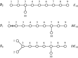
Figure 1: Dynkin diagrams defined (for each $n=2,1,0$) by the ten wall forms $w_{i}^{[n]}(\beta^{\mu}),i=1,\ldots,10$ that determine the billiard dynamics, near a cosmological singularity, of the three blocks of theories ${\cal B}_{2}=\{$M, IIA, IIB$\}$, ${\cal B}_{1}=\{$I, HO, HE$\}$ and ${\cal B}_{0}=\{D=10$ closed bosonic$\}$. The node labels $1,\ldots,10$ correspond to the form label $i$ used in the text.

The corresponding Coxeter diagrams are obtained from the Dynkin diagrams by forgetting about the norms of the wall forms, i.e., by deleting the arrow in $BE_{10}$. As can be seen from the figure, the Dynkin diagrams associated with the billiards turn out to be the Dynkin diagrams of the following rank-$10$ hyperbolic Kac-Moody algebras (see [35]): E₁₀, BE₁₀ and DE₁₀ (for ${\cal B}_{2}$, ${\cal B}_{1}$ and ${\cal B}_{0}$, respectively). It is remarkable that the three billiards exhaust the only three possible simplex Coxeter diagrams on $H^{9}$ with discrete associated Coxeter group (and this is the highest dimension where such simplices exist) [36]. This analysis suggests to identify the 10 wall forms $w_{i}^{[n]}(\beta)$, $i=1,\ldots,10$ of the billiards ${\cal B}_{2}$, ${\cal B}_{1}$ and ${\cal B}_{0}$ with a basis of simple roots of the hyperbolic Kac-Moody algebras E₁₀, BE₁₀ and DE₁₀, so that the cosmological billiard can be identified with a fundamental Weyl chamber of these algebras. Note also that the 10 dynamical variables ${\it\beta^{\mu}}$, $\mu=1,\ldots,10$, can be considered as parametrizing a generic vector in the Cartan subalgebra of these algebras.

It was conjectured some time ago [37] that E₁₀ should be, in some sense, the symmetry group of SUGRA₁₁ reduced to one dimension (and that DE₁₀ be that of type I SUGRA₁₀, which has the same bosonic spectrum as the bosonic string). Our results, which indeed concern the one-dimensional “reduction”, à la BKL, of $M$/string theories exhibit a clear sense in which E₁₀ lies behind the one-dimensional evolution of the block ${\cal B}_{2}$ of theories: their asymptotic cosmological evolution as $t\rightarrow 0$ is a billiard motion, and the group of reflections in the walls of this billiard is nothing else than the Weyl group of E₁₀ (i.e. the group of reflections in the hyperplanes corresponding to the roots of E₁₀, which can be generated by the 10 simple roots of its Dynkin diagram). It is intriguing – and, to our knowledge, unanticipated (see, however, [38])– that the cosmological evolution of the second block of theories, ${\cal B}_{1}=\{$I, HO, HE$\}$, be described by another remarkable billiard, whose group of reflections is the Weyl group of BE₁₀. The root lattices of E₁₀ and BE₁₀ exhaust the only two possible unimodular even and odd Lorentzian 10-dimensional lattices [35].

A first consequence of the exceptional properties of the billiards concerns the nature of the cosmological oscillatory behaviour. They lead to a direct technical proof that these oscillations, for all three blocks, are chaotic in a mathematically well-defined sense. This is done by reformulating, in a standard manner, the billiard dynamics as an equivalent collision-free geodesic motion on a hyperbolic, finite-volume manifold (without boundary) ${\cal M}$ obtained by quotienting $H^{9}$ by an appropriate torsion-free discrete group. These geodesic motions define the “most chaotic” type of dynamical systems. They are Anosov flows [39], which imply, in particular, that they are “mixing”. In principle, one could (at least numerically) compute their largest, positive Lyapunov exponent, say $\lambda^{[n]}$, and their (positive) Kolmogorov-Sinai entropy, say $h^{[n]}$. As we work on a manifold with curvature normalized to $-1$, and walls given in terms of equations containing only numbers of order unity, these quantities will also be of order unity. Furthermore, the two Coxeter groups of E₁₀ and BE₁₀ are the only reflective arithmetic groups in $H^{9}$ [36] so that the chaotic motion in the fundamental simplices of E₁₀ and BE₁₀ will be of the exceptional “arithmetical” type [40]. We therefore expect that the quantum motion on these two billiards, and in particular the spectrum of the Laplacian operator, exhibits exceptional features (Poisson statistics of level-spacing,$\ldots$), linked to the existence of a Hecke algebra of mutually commuting, conserved operators. Another (related) remarkable feature of the billiard motions for all these blocks is their link, pointed out above, with Toda systems. This fact is probably quite significant, both classically and quantum mechanically, because Toda systems whose walls are given in terms of the simple roots of a Lie algebra enjoy remarkable properties. We leave to future work a study of our Toda systems which involve infinite-dimensional hyperbolic Lie algebras.

The discovery that the chaotic behaviour of the generic cosmological solution of superstring effective Lagrangians was rooted in the fundamental Weyl chamber of some underlying hyperbolic Kac-Moody algebra prompted us to reexamine the case of pure gravity [13]. It was found that the same remarquable connection applies to pure gravity in any dimension $D\equiv d+1\geq 4$. The relevant Kac-Moody algebra in this case is $AE_{d}$. It was also found that the disappearance of chaos in pure gravity models when $D\geq 11$ dimensions [30] becomes linked to the fact that the Kac-Moody algebra $AE_{d}$ is no longer “hyperbolic” for $d\geq 10$ [13].

The present investigation a priori concerned only the “low-energy” $(E\ll(\alpha^{\prime})^{-1/2})$, classical cosmological behaviour of string theories. In fact, if (when going toward the singularity) one starts at some “initial” time $t_{0}\sim(d\beta/dt)_{0}^{-1}$ and insists on limiting the application of our results to time scales $|t|\lower 2.15277pt\hbox{$\;\buildrel>\over{\sim}\;$}(\alpha^{\prime})^{1/2}\equiv t_{s}$, the total number of “oscillations”, i.e. the number of collisions on the walls of our billiard will be finite, and will not be very large. The results above show that the number of collisions between $t_{0}$ and $t\rightarrow 0$ is of order $N_{{\rm coll}}\sim\ln\tau\sim\ln(\ln(t_{0}/t))$. This is only $N_{{\rm coll}}\sim 5$ if $t_{0}$ corresponds to the present Hubble scale and $t$ to the string scale $t_{s}$. However, the strongly mixing properties of geodesic motion on hyperbolic spaces make it large enough for churning up the fabric of spacetime and transforming any, non particularly homogeneous at time $t_{0}$, patch of space into a turbulent foam at $t=t_{s}$. Indeed, the mere fact that the walls associated with the spatial curvature and the form fields repeatedly rise up (during the collisions) to the same level as the “time” curvature terms $\sim t^{-2}$, means that the spatial inhomogeneities at $t\sim t_{s}$ will also be of order $t_{s}^{-2}$, corresponding to a string scale foam.

Our results on the ${\cal B}_{2}$ theories probably involve a deep (and not a priori evident) connection with those of Ref. [41] on the structure of the moduli space of $M$-theory compactified on the ten torus $T^{10}$, with vanishing 3-form potential (see also [42]). In both cases the Weyl group of E₁₀ appears. In our case it is (partly) dynamically realized as reflections in the walls of a billiard, while in Ref. [41] it is kinematically realized as a symmetry group of the moduli space of compactifications preserving the maximal number of supersymmetries. In particular, the crucial E-type node of the Dynkin diagram of E₁₀ (Fig. 1) comes, in our study and in the case of $M$-theory, from the wall form $w_{10}^{[2]}(\beta)=\beta_{M}^{1}+\beta_{M}^{2}+\beta_{M}^{3}$ associated with the electric energy of the 3-form. By contrast, in [41] the 3-form is set to zero, and the reflection in $w_{10}^{[2]}$ comes from the 2/5 duality transformation (which is a double $T$ duality in type II theories), which exchanges (in $M$-theory) the 2-brane and the 5-brane. As we emphasized above, dimensional reduction transforms kinematical (permutation) walls into dynamical ones. This suggests that there is no difference of nature between our walls, and that, viewed from a higher standpoint (12-dimension ?), they would all look kinematical, as they are in [41]. By analogy, our findings for the ${\cal B}_{1}$ theories suggest that the Weyl group of BE₁₀ is a symmetry group of the moduli space of $T^{9}$ compactifications of $\{$I, HO, HE$\}$.

Perhaps the most interesting aspect of the above “billiard” analysis is to provide hints for a scenario of vacuum selection in string cosmology. If we heuristically extend our (classical, low-energy, tree-level) results to the quantum, stringy $(t\sim t_{s})$ and/or strongly coupled $(g_{s}\sim 1)$ regime, we are led to conjecture that the initial state of the universe is equivalent to the quantum motion in a certain finite volume chaotic billiard. This billiard is (as in a hall of mirrors game) the fundamental polytope of a discrete symmetry group which contains, as subgroups, the Weyl groups of both E₁₀ and BE₁₀ [43]. We are here assuming that there is (for finite spatial volume universes) a non-zero transition amplitude between the moduli spaces of the two blocks of superstring “theories” (viewed as “states” of an underlying theory). If we had a description of the resulting combined moduli space (orbifolded by its discrete symmetry group) we might even consider as most probable initial state of the universe the fundamental mode of the combined billiard, though this does not seem crucial for vacuum selection purposes. This picture is a generalization of the picture of Ref. [45] (as well as, in some sense, of the “stochastic” PBB picture reviewed above) and, like the latter, might solve the problem of cosmological vacuum selection in allowing the initial state to have a finite probability of exploring the subregions of moduli space which have a chance of inflating and evolving into our present universe.

Acknowledgments: I would like to congratulate Marc Henneaux (Francqui Prize, 2000) for a well deserved recognition, and to thank him for a most pleasant, enriching and fruitful collaboration. I wish also to thank Marc Henneaux and Alexander Sevrin for organizing an extremely stimulating meeting, and the Francqui Foundation for sponsoring in such an elegant and generous manner this very timely colloquium.

References

- [1] M.B. Green, J.H. Schwarz and E. Witten, Superstring theory (Cambridge University Press, Cambridge, 1987).
- [2] J. Polchinski, String Theory, (Cambridge Univ. Press, Cambridge, 1998), 2 volumes; see erratum at www.itp.ucsb.edu/ joep/bigbook.html, in particular the correction of the misprint in Eq. (12.1.34b).
- [3] T.R. Taylor and G. Veneziano, Phys. Lett. B213 (1988) 459.
- [4] T. Damour and A.M. Polyakov, Nucl. Phys. B423 (1994) 532 and Gen. Rel. Grav. 26 (1994) 1171; T. Damour and A. Vilenkin, Phys. Rev. D53 (1996) 2981.
- [5] T. Damour, F. Piazza and G. Veneziano, in preparation.
- [6] G. Veneziano, Phys. Lett. B265, 287 (1991); M. Gasperini and G. Veneziano, Astropart. Phys. 1, 317 (1993); Mod. Phys. Lett. A8, 3701 (1993); Phys. Rev. D50, 2519 (1994).
- [7] An updated collection of papers on the pre-big bang scenario is available at http://www.to.infn.it/~gasperin/.
- [8] J. E. Lidsey, D. Wands and E. J. Copeland, Phys. Rept. 337, 343-492 (2000).
- [9] A. Buonanno, T. Damour and G. Veneziano, Nucl. Phys. B 543, 275 (1999).
- [10] T. Damour and M. Henneaux, Phys. Rev. Lett. 85, 920 (2000); and Gen. Rel. Grav. 32, 2339 (2000).
- [11] T. Damour and M. Henneaux, Phys. Lett. B488, 108 (2000).
- [12] T. Damour and M. Henneaux, Phys. Rev. Lett. 86, 4749 (2001).
- [13] T. Damour, M. Henneaux, B. Julia and H. Nicolai, Phys. Lett. B509, 323 (2001).
- [14] T. Damour, M. Henneaux, and H. Nicolai, in preparation.
- [15] B.A. Campbell, A.D. Linde and K.A. Olive, Nucl. Phys. B355 (1991) 146; R. Brustein and P.J. Steinhardt, Phys. Lett. B302 (1993) 196.
- [16] M.S. Turner and E.J. Weinberg, Phys. Rev. D56 (1997) 4604.
- [17] N. Kaloper, A. Linde and R. Bousso, Phys.Rev.D59 043508 (1999).
- [18] J. Khoury, B. A. Ovrut, N. Seiberg, P. J. Steinhardt,and N. Turok, hep-th/0108187.
- [19] N. Seiberg, these proceedings; hep-th/0201039.
- [20] N. Nekrasov, hep-th/0203112.
- [21] V.P. Frolov, M.A. Markov and V.K. Mukhanov, Phys. Lett. B216 (1989) 272; Phys. Rev. D41 (1990) 383.
- [22] V.K. Mukhanov and R. Brandenberger, Phys. Rev. Lett. 68 (1992) 1969; R. Brandenberger, V.K. Mukhanov and A. Sornborger, Phys. Rev. D48 (1993) 1629.
- [23] L. Smolin, Class. Quant. Grav. 9 (1992) 173.
- [24] V.A. Belinskii and I.M. Khalatnikov, Sov. Phys. JETP 30 (1970) 1174; I.M. Khalatnikov and E.M. Lifshitz, Phys. Rev. Lett. 24 (1970) 76; V.A. Belinskii, E.M. Lifshitz and I.M. Khalatnikov, Sov. Phys. Uspekhi 13 (1971) 745; V.A. Belinskii, E.M. Lifshitz and I.M. Khalatnikov, Adv. Phys. 19, 525 (1970); and Adv. Phys. 31, 639 (1982).
- [25] V.A. Belinskii and I.M. Khalatnikov, Sov. Phys. JETP 36 (1973) 591.
- [26] L. Andersson and A.D. Rendall, Commun. Math. Phys. 218, 479 (2001).
- [27] T. Damour, M. Henneaux, A. D. Rendall, and M. Weaver, gr-qc/0202069.
- [28] E.M. Lifshitz, I.M. Lifshitz and I.M. Khalatnikov, Sov. Phys. JETP 32, 173 (1971); D.F. Chernoff and J.D. Barrow, Phys. Rev. Lett. 50, 134 (1983); I.M. Khalatnikov, E.M. Lifshitz, K.M. Kanin, L.M. Shchur and Ya.G. Sinai, J. Stat. Phys. 38, 97 (1985); N.J. Cornish and J.J. Levin, Phys. Rev. D 55, 7489 (1997).
- [29] B. K. Berger, D. Garfinkle, J. Isenberg, V. Moncrief and M. Weaver, Mod. Phys. Lett. A13, 1565 (1998).
- [30] J. Demaret, M. Henneaux and P. Spindel, Phys. Lett. 164B, 27 (1985); J. Demaret, Y de Rop and M. Henneaux, Int. J. Theor. Phys. 28, 1067 (1989).
- [31] D.M. Chitre, Ph. D. thesis, University of Maryland, 1972.
- [32] C.W. Misner, in D. Hobill et al. (Eds), Deterministic chaos in general relativity, (Plenum, 1994) pp. 317-328.
- [33] V. D. Ivashchuk, V. N. Melnikov and A. A. Kirillov, JETP Lett. 60, 235 (1994).
- [34] We included for the sake of comparison the bosonic string model in . Though is not the critical dimension of the quantum bosonic string, it is the critical dimension above which the never ending oscillations in its cosmological evolution disappear [11].
- [35] V.G. Kac, Infinite dimensional Lie algebras, third edition (Cambridge University Press, 1990).
- [36] E.B. Vinberg (Ed.), Geometry II, Encyclopaedia of Mathematical Sciences, vol. 29 (Springer-Verlag, 1993).
- [37] B. Julia, in Lectures in Applied Mathematics, AMS-SIAM, vol. 21, (1985), p. 335.
- [38] E. Cremmer, B. Julia, H. Lu and C.N. Pope, hep-th/9909099
- [39] D.V. Anosov, Proc. Steklov Inst. N. 90 (1967).
- [40] E.B. Bogomolny, B. Georgeot, M.J. Giannoni and C. Schmit, Phys. Rep. 291 (5 & 6) 219-326 (1997).
- [41] T. Banks, W. Fischler and L. Motl, JHEP 01, 019 (1999).
- [42] N. A. Obers and B. Pioline, Phys. Rept. 318 (1999) 113.
- [43] With -theory [44] in mind, it is tempting to look for a Kac-Moody algebra with ultra-hyperbolic signature containing both E10 and BE10. According to V. Kac (private communication) the smallest such algebra is the rank- algebra whose Dynkin diagram is obtained by connecting, by a simple line, the and nodes in Fig. 1.
- [44] C. Vafa, Nucl. Phys. B469, 403 (1996).
- [45] J.H. Horne and G. Moore, Nucl. Phys. B432, 109 (1994).