Discrete Torsion in Singular $G_{2}$-Manifolds and Real LG

Abstract

We investigate strings at singularities of $G_{2}$-holonomy manifolds which arise in ${\mathbb{Z}}_{2}$ orbifolds of Calabi-Yau spaces times a circle. The singularities locally look like ${\mathbb{R}}^{4}/{\mathbb{Z}}_{2}$ fibered over a SLAG, and can globally be embedded in CICYs in weighted projective spaces. The local model depends on the choice of a discrete torsion in the fibration, and the global model on an anti-holomorphic involution of the Calabi-Yau hypersurface. We determine how these choices are related to each other by computing a Wilson surface detecting discrete torsion. We then follow the same orbifolds to the non-geometric Landau-Ginzburg region of moduli space. We argue that the symmetry-breaking twisted sectors are effectively captured by real Landau-Ginzburg potentials. In particular, we find agreement in the low-energy spectra of strings computed from geometry and Gepner-model CFT. Along the way, we construct the full modular data of orbifolds of ${\cal N}=2$ minimal models by the mirror automorphism, and give a real-LG interpretation of their modular invariants. Some of the models provide examples of the mirror-symmetry phenomenon for $G_{2}$ holonomy.

©  2002 International Press

Adv. Theor. Math. Phys. 6 (2002) 207–278

Department of Physics University of California Santa Barbara, CA 93106, USA roiban@vulcan.physics.ucsb.edu Department of Physics and CIT-USC Center for Theoretical Physics University of Southern Calfornia Los Angeles, CA 90089, USA roemel@citusc.usc.edu Institute for Theoretical Physics University of California Santa Barbara, CA 93106, USA walcher@itp.ucsb.edu

1 Introduction and Summary

In this paper, we study strings on $G_{2}$-holonomy spaces with orbifold singularities. The examples we analyze are representable as ${\mathbb{Z}}_{2}$ quotients of Calabi-Yau threefolds times a circle, and in certain cases are singular limits of smooth $G_{2}$-manifolds.

Such $G_{2}$-holonomy spaces with singularities play a fundamental role in phenomenologically relevant compactifications of M-theory to four dimensions, see [3, 4, 5, 6, 7, 8, 9, 10, 11] and references thereto. In these references, it is shown how ADE-singularities in codimension $4$ give rise to non-abelian gauge symmetries [5, 6], and extra isolated singularities, to chiral fermions [8, 11], in the low-energy effective theory in four dimensions. The resulting dynamics can sometimes be solved and this has led to a number of interesting insights concerning geometric realizations of phase transitions in field theory. In the present paper, however, we will put aside these perspectives of $G_{2}$ holonomy, and rather try to understand certain aspects of stringy geometry associated with exceptional holonomy, following [1, 2, 26, 27, 28, 29].

To pose the basic problem that is addressed in this paper, we consider, as an example, the Calabi-Yau hypersurface

$$Y=\{[x_{i}];x_{1}^{8}+x_{2}^{8}+x_{3}^{8}+x_{4}^{8}+x_{5}^{2}=0\}$$ (1)

in the complex weighted-projective space ${\mathbb{P}}_{11114}^{4}$. We also have in mind an anti-holomorphic involution of $Y$ such as

$$\omega:x_{i}\mapsto{\bar{x}}_{i}\,,$$ (2)

and are interested in the quotient $X=\frac{Y\times S^{1}}{\omega}$, where $\omega$ acts as (2) on $Y$ and as inversion on the circle. The holonomy of $X$ is strictly larger than SU$(3)$, and the next available Lie group on Berger’s list is $G_{2}$. We will losely refer to such $X$ as a $G_{2}$-holonomy space.

Compactification of the type II string on $X$ will lead in three dimensions to a theory with ${\cal N}=2$ supersymmetry. In the large-volume limit, we can determine the massless spectrum of this theory from the classical geometry, or actually just the topology, of $X$. Let us focus on the symmetry-breaking twisted sectors of the orbifold. To obtain massless twisted strings, we would need $\omega$ to have fixed points. But $\omega$ acts freely on $Y\times S^{1}$, simply because there are no real points on $Y$! So in this example, we do not expect any massless strings from the twisted sector.

As we now let $X$ shrink in size, stringy effects become important and classical geometry is less useful. In the small-volume limit, a much better description is in terms of Landau-Ginzburg theory [30, 31, 32, 33, 34]. For $Y$ at hand, the relevant LG model is given by the superpotential

$$W=x_{1}^{8}+x_{2}^{8}+x_{3}^{8}+x_{4}^{8}\,,$$ (3)

where the $x_{i}$’s are complex ${\cal N}=2$ LG fields, and a ${\mathbb{Z}}_{8}$ orbifold is implicit. This potential is related in the obvious way to the polynomial in (1) by integrating out the massive field $x_{5}$. Let us again look at the $\omega$-twisted sector of the orbifold. For massless strings, the twisted boundary conditions set the imaginary part of the $x_{i}$’s to zero, and we obtain the restriction of $W$ to real $x_{i}$’s. It is not hard to determine the groundstates for this real LG potential. One finds in particular the Witten index in the twisted sector to be ${{\mathop{\rm tr}}_{\rm tw}(-1)^{F}}=1$, in clear contradiction to the geometric result, which was $0$.

Of course, our argument relies on Landau-Ginzburg theory with ${\cal N}<2$ supersymmetries, and it can not be taken for granted that the correspondence with geometry extends to this situation. However, since we are at the Fermat point in LG moduli space, we can also use the exactly solvable Gepner-model CFT [35, 36] based on tensor products of ${\cal N}=2$ minimal models. Indeed, it has been found in [27, 28] that there can be massless modes in the twisted sectors of the corresponding orbifolds precisely if all levels of the minimal models are even. The model corresponding to (1) is an example of this [26], with levels $(6,6,6,6)$. Hence, also the Gepner model seems to contradict the geometrical result.

In fact, since the theory in three dimensions has only 4 supercharges, one might also imagine that there is a superpotential with a non-geometric branch opening up at the Landau-Ginzburg point. This, however, is to be ruled out by the basic result of Shatashvili and Vafa [1] that the extended chiral algebra associated with $G_{2}$ holonomy suffices to protect marginal operators in conformal field theory. The role that in the ${\cal N}=2$ situation is played by the U$(1)$ current is here taken over by the tri-critical Ising model. It generates the extension beyond ${\cal N}=1$ worldsheet supersymmetry, and can be used to show, relying on results of [37], that any marginal operator is exactly marginal.

The apparent discrepancy between geometry and the Gepner model was first pointed out in [26]. Actually, there is a related puzzle, also noticed in [26], which arises if $Y$ is replaced with the quintic. Indeed, all levels in the Gepner model are then odd, and there is no twisted massless mode. However, at large volume, the fixed point locus of the involution is a non-trivial ${\mathbb{R}}{\mathbb{P}}^{3}$ and an “adiabatic argument” would imply a massless vector multiplet in three dimensions.

It was proposed in [26] that a solution of these puzzles might be related to the fact that the Gepner models typically lie on the $B=\frac{1}{2}$ line in Kähler moduli space, while the geometry naturally has $B=0$. In the ${\mathbb{Z}}_{2}$ orbifold these two branches become disconnected, and the spectra need not agree. However, a satisfactory dynamical explanation of the lifting of modes has not been given so far. In particular, one needs to explain why the extra modes appear sometimes on the $B=\frac{1}{2}$ (as for $X$), and sometimes on the $B=0$ branch (as for the quintic).

We will show that the discrepancies actually disappear after a careful analysis of the orbifold action, in particular on the B-field. Indeed, there are several topologically distinct orbifolds, both in the geometry and in the LG/Gepner model. The spectra in the twisted sector depend on the model, but agree after a proper identification of the orbifolds at large and small volume. The B-field, both through the bulk Calabi-Yau space and through the orbifold in the form of discrete torsion, plays a crucial role in the analysis.

We now summarize the main results of the paper. The basic observation that will solve the above puzzle is that the involution (2) can be twisted by the phase symmetries of the defining equation in (1), i.e., $x_{i}\mapsto{\rm e}^{2\pi{\rm i}M_{i}/8}{\bar{x}}_{i}\,$, and that for a suitable choice of phases, the fixed point set is determined by the real equation

$$\pm{\xi}_{1}^{8}\pm{\xi}_{2}^{8}\pm{\xi}_{3}^{8}\pm{\xi}_{4}^{8}\pm{\xi}_{5}^{2}=0\,.$$ (4)

The topology of the fixed point set does depend on the signs in (4) and certainly does not always exclude massless twisted strings. We will describe these possibilities in more details, and for more general models, in section 2. On the conformal field theory side, the existence of massless fields is really a result from the representation theory of the chiral algebra, which is the chiral algebra of the Gepner model divided by $\omega$. More precisely, the Ramond ground states associated with the massless fields appear at the level of the indivdual minimal models. But this does not imply that these fields are actually contained in any modular invariant built on this chiral algebra. We will see in sections 6 and 7 that there are indeed modular invariants in which the Ramond ground states are absent.

The technical core of our paper can be found in sections 3 through 6. Basically, the local geometry of the singularity is the fibration of an $A_{1}$ singularity over a supersymmetric three-cycle. Similarly to geometric engineering [38, 39, 40], we first compactify the IIA string on the ALE space, which leads to an ${\cal N}=(1,1)$ gauge theory in six dimensions, at a generic point on the Coulomb branch [41]. We then compactify further down to three dimensions. In order to preserve supersymmetry, the theory has to be twisted by a non-trivial R-symmetry connection [42]. However, it turns out that there is the possibility of an additional discrete twist by a real line bundle that couples to the quantum symmetry of the ALE space at the orbifold point in its moduli space. In particular, this twist can lift massless modes that would have been expected from topological twisting.

In section 4, we show how this discrete twist, which we identify with discrete torsion [43], arises in the global model. Following suggestions by Sharpe [44, 45, 46], we detect the discrete torsion by computing a Wilson surface in the covering space of the orbifold, i.e., an integral $\int_{\hat{\Sigma}}B$, where $\hat{\Sigma}$ is the covering of a torus worldsheet inside $Y\times S^{1}$. The non-trivial contribution to this Wilson surface comes from a boundary gluing term, which we show is non-zero precisely because $B=\frac{1}{2}$ on the Calabi-Yau space. We perform explicit calculations for three examples, the quintic, ${\mathbb{P}}_{11114}^{4}[8]$, and ${\mathbb{P}}_{11222}^{4}[8]$—some of them in appendix A—but our methods are generalizable to other models.

We then leave geometry for a while and turn to a detailed study of orbifolds of ${\cal N}=2$ minimal models by antiholomorphic involutions. Having obtained the full modular data of the chiral theories in section 5, we illustrate in section 6 the somewhat surprising connection between the twisted sectors of these orbifolds and real Landau-Ginzburg potentials. This connection will be the basic tool to compute the string spectrum on the $G_{2}$-spaces at small volume. We emphasize, however, that the details of sections 5 and 6, except possibly subsection 6.2, are not essential for an understanding of the geometrical parts of the paper.

We are then finally ready in section 7 for the study of the (non-abelian) Landau-Ginzburg orbifolds that describe the small-volume regime of our $G_{2}$-holonomy spaces. We introduce an index that counts the total number of ground states, and discuss the notion of Poincaré duality in this context. We derive the massless spectra of twisted strings in this framework and show that they agree with the geometrical results.

We end with a speculation concerning mirror symmetry for $G_{2}$-holonomy manifolds. In [1] it was argued that mirror symmetry should be viewed as the inaptitude of conformal field theory to completely decipher the geometry of the target space. For $G_{2}$ holonomy, strings can only detect the sum of Betti numbers $b_{2}+b_{3}$, but not $b_{2}$ or $b_{3}$ independently. This is similar to the mirror-symmetry phenomenon for Calabi-Yau threefolds, in which the Hodge numbers $h_{11}$ and $h_{21}$ can be determined from string theory only up to their exchange. More generally, if we take into account that discrete fluxes can lift modes from the naively expected massless spectrum, we are led to classify under mirror symmetry any collection of classical geometries with or without discrete fluxes that yield isomorphic conformal field theories when probed with strings. We will show that this phenomenon indeed appears in the situations studied in this paper.

For an example, let us return to the manifold $X$, and to the relation between geometry and Landau-Ginzburg model. The continuation from large to small volume or vice-versa involves integrating-out or integrating-in the massive LG field $x_{5}$. In so doing, the phase of the quadratic piece in the potential is not determined, since it can simply be removed by redefinition of $x_{5}$. However, after quotienting by the involution $\omega$, a sign in front of ${\xi}_{5}^{2}$, with ${\xi}_{5}$ now real, can not be removed by a real change of variables. And indeed, the two real sections of $Y$, given by $\sum_{i}{\xi}_{i}^{8}\pm{\xi}_{5}^{2}=0$, respectively, have distinct topologies. For $\pm=+$ the fixed point set of $\omega$ is empty, while for $\pm=-$, it consists of two copies of the real projective space ${\mathbb{R}}{\mathbb{P}}^{3}$. So we have precisely the situation in which two distinct classical geometries lead at small volume to indistinguishable theories. Of course, to match the spectra, one has to take into account the discrete fluxes that thread the large-volume cycles for one choice of signs. It is clear that this sort of mirror symmetry is a rather common phenomenon in our context. More examples will become clear in section 7, including ones with massless modes in the twisted sector. It will be interesting to see if they can be extended to full-fledged mirror symmetries.

2 Orbifolds of $G_{2}$ Holonomy

String compactification to $3$ dimensions with minimal supersymmetry requires the compactification space to have $G_{2}$ holonomy, just as $4$ dimensions require SU$(3)$ holonomy. It is a natural question to ask how much of the usual Calabi-Yau story can be extended to $G_{2}$ holonomy [1]. An important step in this program is the construction of examples of manifolds admitting $G_{2}$-holonomy metrics [47, 48]. While most of the recent progress on this issue is being made in the non-compact situation [15, 16, 17, 18, 19, 20], interesting physics is likely to emerge with compact $G_{2}$-manifolds, also from the M-theory perspective [10, 21]. In a sense the simplest compact $G_{2}$-manifolds can be obtained from orbifolding Calabi-Yau threefolds [49], as discussed in the CFT framework in [2].

2.1 $G_{2}$-manifolds from Calabi-Yau spaces

A 7-manifold with $G_{2}$ holonomy has a covariantly constant, so-called associative, 3-form which locally looks like [50]

$$\phi=dx^{567}+dx^{5}(dx^{12}-dx^{34})+dx^{6}(dx^{13}+dx^{24})+dx^{7}(dx^{14}-dx^{23})\,.$$ (5)

More precisely, written in this way, $\phi$ distinguishes a $G_{2}$ subgroup of SO$(7)$ as its isotropy group, and is hence covariantly constant if the holonomy is in $G_{2}$. We may embed ${\rm SO}(4)={\rm SU}(2)\times{\rm SU}(2)$ into SO$(7)$ by acting on the first four coordinates by a normal rotation $(2,2)$ and on the last three coordinates as if they were anti-self-dual forms $(1,3)$. Then (5) shows that SO$(4)$ is a subgroup of $G_{2}$.

Another maximal subgroup of $G_{2}$ is SU$(3)$. If a Calabi-Yau space $Y$ admits an antiholomorphic involution $\omega$ as an isometry, then $X=\frac{Y\times S^{1}}{{\mathbb{Z}}_{2}}$ with the ${\mathbb{Z}}_{2}$ action being the combined action of $\omega$ and $x\mapsto-x$ on the circle is a manifold of $G_{2}$ holonomy. The associative 3-form is then

$$\phi=J\wedge dx+{\rm Re\hskip 1.00006pt}(\Omega)\,,$$ (6)

where $J$ is the Kähler form on $Y$ and $\Omega$ is the holomorphic 3-form. The phase of $\Omega$ is fixed up to multiplication with $-1$ by the requirement that $\Omega\mapsto\bar{\Omega}$ under $\omega$. The sign ambiguity of $\Omega$ can be fixed by reversing the orientation of the $S^{1}$ and the fact that $\phi$ is only defined up to a nonvanishing real factor.

Singularities in $X$ arise if $\omega$ has fixed points. By construction, the fixed point locus in $Y$ is a special Lagrangian submanifold, $M$. The singular set of $X$ then consists of two copies of $M$ because of the two fixed points on $S^{1}$. The local geometry of $Y$ around $M$ is described by the normal bundle $NM$ of $M\subset Y$. The complex structure on $Y$ identifies the normal bundle $NM$ with the tangent bundle $TM$ by multiplication with the imaginary unit. Thus, the local structure of such a singular locus in $X$ is $X_{L}=\frac{TM\times{\mathbb{R}}}{{\mathbb{Z}}_{2}}$ with the ${\mathbb{Z}}_{2}$ acting on the ${\mathbb{R}}^{4}$ fiber of $TM\times{\mathbb{R}}$ by reflection at the origin. This is a singular $A_{1}$ fibration over $M$.

The massless spectrum of type IIA string theory on a $G_{2}$-manifold $X$ consists of three kinds of multiplets in three dimensions. The gravity multiplet contains the graviton and the RR-1-form $C_{\mu}$. Like in four dimensions, the dilaton sits in a universal multiplet, which is a chiral multiplet in three dimensions. The remainder of the vector- and chiral-multiplet spectrum depends strongly on the choice of the $X$.

If $X$ were nonsingular, we would obtain the usual spectrum of string theory after Kaluza-Klein reduction. This leads to $b_{2}(X)$ vector multiplets, due to the B-field and the RR-3-form, and $b_{3}(X)$ chiral multiplets, due to the metric deformations and the RR-3-form.

With the help of electric-magnetic duality, massless abelian vector multiplets and chiral multiplets can be converted into each other. From the point of view of 10-dimensional electric-magnetic duality, only the exchange of all vector and all chiral multiplets seems natural, but from the three-dimensional point of view, we might also think about dualizing individual multiplets. This is mirror symmetry in three dimensions [51, 52, 53, 54]. Mirror symmetry for $G_{2}$-manifolds is similar to this [1, 55, 56, 57]. As defined in [1], $G_{2}$-manifolds are mirror to one another if the sigma models on them give rise to identical conformal field theories. This implies that $b_{2}+b_{3}$ must be constant within a mirror family (which typically has more than two members). So switching the geometric interpretation of the same conformal field theory typically entails the exchange of a chiral with a vector multiplet.

In our example of $X=\frac{Y\times S^{1}}{{\mathbb{Z}}_{2}}$, the Betti numbers of $X$ can be determined from the Hodge numbers of $Y$ and the action of $\omega$. For example, $H^{2}(Y)$ splits into positive and negative eigenspaces of $\omega$, $H_{+}^{2}(X)$ and $H_{-}^{2}(X)$, which are invariant when combined with the zeroth and and first cohomology of $S^{1}$, respectively. The split of $H^{3}(Y)=H^{3,0}\oplus H^{2,1}\oplus H^{1,2}\oplus H^{0,3}$ leads to equal dimensions of positive and negative eigenspaces. This gives the Betti numbers from the untwisted sector

$$\begin{split}b^{(u)}_{2}(X)&=h_{1,1}^{+}\,,\\ b^{(u)}_{3}(X)&=h_{1,1}^{-}+h_{2,1}+1\,.\end{split}$$ (7)

The massless untwisted 3-dimensional spectrum of type IIA theory on $X$ is then given by $b^{(u)}_{2}(X)$ vector multiplets together with $b^{(u)}_{3}(X)$ chiral multiplets. As for the twisted sector, the “shrunk 2-cycle” of the $A_{1}$ fibers can be combined with the $0$- and $1$-cycles of the fixed point locus $M$. As we will see in section 3.1, one gets ${\hat{b}}_{0}(M)$ vector and ${\hat{b}}_{1}(M)$ chiral multiplets, where ${\hat{b}}_{i}(M)$ are certain twisted Betti numbers of $M$. The chiral multiplets in the twisted sector correspond to blowup modes for the singular locus, whereas the scalars in vector multiplets correspond to the B-field flux through the shrunk $S^{2}$ of the $A_{1}$ fiber.

2.2 Involutions and GLSM

Many examples of Calabi-Yau manifolds can be realized as complete intersections in weighted-projective spaces, and it is natural to ask what the resulting $G_{2}$-holonomy geometries are, both at large and at small volume. The natural framework for this is the gauged linear sigma model (GLSM) [34]. At large volume, the GLSM reduces at low energies to the non-linear sigma model, while at small volume, we obtain a Landau-Ginzburg orbifold.

Such a gauged linear sigma model has a number of U$(1)$ gauge groups and chiral fields $x_{i}$ with charges $w_{i}^{(a)}$ together with a gauge invariant superpotential $W(x_{i})$. A possible antiholomorphic involution $\omega$ has to preserve the U$(1)$ gauge invariance and the superpotential. In order to preserve the flat metric and the origin on the space of the $x_{i}$, the involution $\omega$ has to act by a unitary transformation as

$$\omega:x_{i}\mapsto M_{ij}\bar{x}_{j}\,.$$ (8)

Gauge invariance requires $M_{ij}$ to be block diagonal, where the U$(1)$ charges in one block are all the same. Furthermore, $M_{ij}$ can be ’rotated’ by U$(1)$ gauge transformations.

Further restrictions on $M_{ij}$ follow from the requirement that the superpotential $W$ be ’invariant’ under $\omega$,

$$W(M_{ij}\bar{x}_{j})=\overline{W(x_{j})}\,.$$ (9)

We will not try to classify those antiholomorphic involutions, but rather want to understand the ones where $M_{ij}$ is diagonal. There are in general more complicated involutions, which for example permute some $x_{i}$ with the same U$(1)$ charges [12].

For simplicity, let us restrict ourselves to the case of a single U$(1)$ gauge group, five chiral superfields $x_{i}$ with charges $w_{i}$ and one chiral superfield $p$ of charge $w=-\sum w_{i}$. We take the superpotential to be

$$W=p\sum_{i}x_{i}^{h_{i}}\,.$$ (10)

The antiholomorphic involution is of the form

$$(x_{1},\ldots,x_{5},p)\mapsto(\rho_{1}\bar{x}_{1},\ldots,\rho_{5}\bar{x}_{5},\rho\bar{p})\,,$$ (11)

where the condition (9) puts certain constraints on the phases $\rho_{i}$,

$$\rho_{i}^{h_{i}}=\rho^{-1}\,.$$ (12)

We can use gauge transformations to fix $\rho=1$. Then the $\rho_{i}$ are $h_{i}$-th roots of unity. The involution (11) can then be viewed as the involution $x_{i}\mapsto\bar{x}_{i}$ together with the discrete global symmetry $x_{i}\mapsto\rho_{i}x_{i}$ of the theory. It is, however, not true that we can always remove the phases $\rho_{i}$ by a symmetry transformation. Indeed, the involution (11) acts on $\rho_{i}^{\prime}x_{i}$ as $\rho_{i}^{\prime}x_{i}\mapsto\rho_{i}(\rho_{i}^{\prime})^{-1}\bar{x}_{i}$ or equivalently as $x_{i}\mapsto\rho_{i}(\rho_{i}^{\prime})^{-2}\bar{x}_{i}$. This shows that two involutions are related by symmetry if and only if the $\rho_{i}$ differ by even powers of an $h_{i}$-th root of unity. For each even $h_{i}$, this leaves two essentially different choices for $\rho_{i}$, whereas if $h_{i}$ is odd all choices of $\rho_{i}$ are equivalent. Furthermore, two choices are equivalent if they differ by a residual gauge transformation, i.e., $\rho_{i}\mapsto{\rm e}^{2\pi{\rm i}/h_{i}}\rho_{i}$ for all $i$ simultaneously.

The gauged linear sigma model can now be used to relate the action of the antiholomorphic involution $\omega$ in the Calabi-Yau phase to the action in the Landau-Ginzburg phase. In the Calabi-Yau phase we have a hypersurface given by the equation $\sum x_{i}^{h_{i}}=0$ in a weighted-projective space ${\mathbb{P}}_{(w_{1},\ldots,w_{5})}^{4}$, and in the Landau-Ginzburg phase we get a ${\mathbb{Z}}_{h}$ Landau Ginzburg orbifold (where $h={\rm lcm}(h_{i})$ and $w_{i}=h/h_{i}$). The involutions act in both limits in the obvious way by $x_{i}\mapsto\rho_{i}\bar{x}_{i}$.

3 Local Model

The $G_{2}$-manifold $X=\frac{Y\times S^{1}}{{\mathbb{Z}}_{2}}$ has singularities where the anti-holomorphic involution $\omega$ has fixed points. The local model for such a singular locus is $X_{L}=\frac{TM\times{\mathbb{R}}}{{\mathbb{Z}}_{2}}$, where $M$ is a supersymmetric 3-cycle. We have seen that this is a singular $A_{1}$ fibration over $M$. String theory is non-singular because a B-field threading the shrunk 2-cycle gives non-zero mass to the branes wrapped around it [41]. This situation is very much reminiscent of geometric engineering, where the fibration of ADE singularities over Riemann surfaces is used to design quantum field theories in 4 dimensions. In this context, an analysis based on topological twisting [42] gives the right answer for the spectrum in 4 dimensions [38]. We will see that the present situation is somewhat more complicated.

3.1 The Topological Twisting

The low-energy theory for type IIA strings on the ${\mathbb{R}}^{4}/{\mathbb{Z}}_{2}$ orbifold is an ${\cal N}=(1,1)$ U$(1)$ gauge theory on the 6-dimensional fixed plane, coupled to the massless 10-dimensional type IIA fields. The SO$(4)$ R-symmetry can be identified with the rotation group transverse to the fixed plane and is gauged for this reason. The SO$(4)$ gauge fields are 10-dimensional (non-normalizable) gravitons which are polarized with one index in the transverse space and one index in the orbifold directions. The field content of the 6-dimensional (twisted) subsector is summarized in the following table.

Field	SO$(5,1)_{t}$	SO$(4)_{r}={\rm SU}(2)_{c}\times{\rm SU}(2)_{a}$
$A_{\mu}$	$6$	$(1,1)$
$\phi$	$1$	$(2,2)$
$\psi$	$4$	$(2,1)$
$\lambda$	$4^{\prime}$	$(1,2)$

The gauge boson $A_{\mu}$ is a RR-field and $\phi$ is in the NSNS-sector. The 6-dimensional action for the bosons has to be consistent with those symmetries and with supersymmetry. The kinetic terms of the 6-dimensional action are

$${\cal A}_{K}=\int d^{6}x\sqrt{-g_{6}}\left[(D_{\mu}\phi)^{2}+(F_{\mu\nu})^{2}\right]\,,$$ (13)

where the derivatives are defined as

$$\begin{array}[]{c}F_{\mu\nu}=\partial_{\mu}A_{\nu}-\partial_{\nu}A_{\mu}\,,\\ D_{\mu}\phi^{i}=\partial_{\mu}\phi^{i}+\omega^{i}{}_{j}{}_{\mu}\phi^{j}\,,\end{array}$$ (14)

with $\omega^{i}{}_{j}{}_{\mu}$ being the SO$(4)$ gauge connection which is induced from the connection on the $A_{1}$ fibration. It has a particular value determined by the supersymmetry condition solved by the geometry of the particular fibration $X_{L}=\frac{TM\times{\mathbb{R}}}{{\mathbb{Z}}_{2}}$.

The familiar topological twisting [42, 38] now instructs us to view this solution of the supersymmetry condition as a result of the embedding of the SO$(3)$ structure group of the tangent bundle $TM$ diagonally into the SO$(4)/{\mathbb{Z}}_{2}$ structure group of $X_{L}$. This also means that the R-symmetry connection is given in terms of the Levi-Civita connection on the special Lagrangian fixed cycle $M$. Under this split, the transformation properties of the different 6-dimensional fields are as follows.

Field	SO$(2,1)_{t}$	SO$(3)_{i}$	SO$(4)_{r}={\rm SU}(2)_{c}\times{\rm SU}(2)_{a}$
$A_{\mu}$	$3$	$1$	$(1,1)$
$A_{i}$	$1$	$3$	$(1,1)$
$\phi$	$1$	$1$	$(2,2)$
$\psi$	$2$	$2$	$(2,1)$
$\lambda$	$2$	$2$	$(1,2)$

The diagonal topological twist retains four supercharges in three dimensions, which are the singlets under the diagonal SO$(3)$. As for the field content, we have the singlets $(A_{\mu},\phi^{(1)},\psi^{(1)},\lambda^{(1)})$ and the triplets $(A_{i},\phi^{(3)},\psi^{(3)},\lambda^{(3)})$. The singlets correspond to scalars on $M$, while the triplets would be one-forms in the usual assignement. Therefore, if we only take into account the topological twist, we predict that the 3-dimensional ${\cal N}=2$ theory has $b_{0}(M)$ vector multiplets and $b_{1}(M)$ chiral multiplets. In particular, this would give one vector multiplet for each connected component of $M$.

However, as remarked in [26], this result seems to be in contradiction to the results from the Gepner-model construction, where one obtains a rather different spectrum of massless fields in the twisted sector. This indicates that the topological twist does not completely capture the topology of all fields involved in the compactification, and we should take a closer look at possible subtleties.

On the one hand, we note that the $A_{1}$ fibration classically has an SO$(4)/{\mathbb{Z}}_{2}$ structure group, but that the R-symmetry group is actually SO$(4)$. So we have to address the question of existence and uniqueness of this lift.

On the other hand, the theory with Lagrangian (13) has, apart from the gauge symmetries, that we discussed, a ${\mathbb{Z}}_{2}$ symmetry which leaves invariant all the 10-dimensional fields and multiplies the twisted 6-dimensional fields by $(-1)$. This is the ${\mathbb{Z}}_{2}$ quantum symmetry of the orbifold CFT. It is unbroken only at the orbifold point, and it is broken in particular at the point of enhanced SU$(2)$ gauge symmetry. In string theory, this ${\mathbb{Z}}_{2}$ symmetry is gauged as well.

We now have to consider what the global field configuration is, including all the continuous and discrete gauge symmetries.

We first look at the lift of the $A_{1}$ bundle to the SO$(4)$ R-symmetry bundle. The existence of the lift is determined by a second cohomology class $\tilde{w}_{2}$ analogous to the second Stiefel-Whitney class [58, 59]. In the examples that we are studying, the local model is $X_{L}=\frac{TM\times{\mathbb{R}}}{{\mathbb{Z}}_{2}}$ and we have the explicit lift to $TM\times{\mathbb{R}}$. For this reason the class $\tilde{w}_{2}$ is vanishing. This lift is not necessarily unique, but the potential ambiguity in the lift to the R-symmetry bundle is fixed by the requirement of unbroken ${\cal N}=2$ supersymmetry in 3 dimensions. Namely, the existence of unbroken supersymmetry requires the Spin$(3)_{i}$, the SU$(2)_{c}\,$, and the SU$(2)_{a}$ bundle all to be the same. This is also the reason why the ambiguity in the Spin$(3)$ bundle is irrelevant. Since all fields transform either trivially under the SO$(3)_{i}\times{\rm SU}(2)_{c}\times{\rm SU}(2)_{a}$ or as a $(2,2,1)$, a $(2,1,2)$ or a $(1,2,2)$, a factor $(-1)$ in the Spin$(3)_{i}$ always gets squared to $1$.

For the ${\mathbb{Z}}_{2}$ quantum symmetry, gauging amounts to the choice of a real line bundle $L$ over $M$. If $L$ is nontrivial, the massless spectrum of twist fields on $M$ is no more described by the ordinary cohomology $H^{*}(M,{\mathbb{R}})$. Because all 6-dimensional fields transform in the non-trivial representation of the quantum ${\mathbb{Z}}_{2}$, the relevant cohomology is now the twisted cohomology $H^{*}(M,L)$, which is quite different as we will see below.

Thus, from a physical point of view, the local model is given not only by the special Lagrangian $M$, but also requires the choice of a real line bundle $L$. One might expect that this line bundle also plays a role from the mathematical point of view in the study of the resolvability of the orbifold singularities to smooth $G_{2}$-manifolds. It should then presumably also enter the proper definition of orbifold cohomology at the singularity.

3.2 Gauging the quantum symmetry as a discrete torsion

Real line bundles on $M$ are classified by $H^{1}(M,{\mathbb{Z}}_{2})$, which is the ${\mathbb{Z}}_{2}$ transition functions modulo equivalence. These transition functions also appear as the (discrete) holonomy around a closed loop $\gamma\subset M$. For example, if there are no non-trivial closed loops in $M$, then all real line bundles are trivial.

This gives a way to determine $L$ in string theory. We simply compute the sign that a twisted string picks up when it propagates around a closed loop $\gamma\subset M$. Such a twisted string propagating around $\gamma$ is a torus diagram embedded in $X_{L}$. Therefore, the holonomy of the real line bundle appears as a sign in front of a particular twisted partition function. In other words, we have a sign associated with a torus wrapping a non-trivial 2-cycle in $X_{L}\setminus M$, that is not determined by modular invariance. This is called discrete torsion [43].

In the local geometries that we are studying, this discrete torsion can also be seen in a bit more conventional orbifold sense. In our examples below, $M$ can be written as a ${\mathbb{Z}}_{2}$ quotient of some covering space $\tilde{M}$. Then the local geometry is $\frac{T\tilde{M}\times{\mathbb{R}}}{{\mathbb{Z}}_{2}\times{\mathbb{Z}}_{2}}$, and the effect of turning on discrete torsion in this ${\mathbb{Z}}_{2}\times{\mathbb{Z}}_{2}$ orbifold corresponds to a non-trivial choice of $L$. In this case, the discrete torsion can be understood in such geometrical terms as a choice of a bundle $L$ over $M$ because the ${\mathbb{Z}}_{2}$ acting on $\tilde{M}$ has no fixed points.

This ${\mathbb{Z}}_{2}\times{\mathbb{Z}}_{2}$ orbifold of $\tilde{M}\times{\mathbb{R}}$ can also be used to calculate the twisted cohomology $H^{*}(M,L)$ from $H^{*}(\tilde{M},{\mathbb{R}})$ by projecting onto invariant forms. We will denote the dimensions of these cohomologies (the twisted Betti numbers) by $\hat{b}_{0}$ and $\hat{b}_{1}$.

For example, consider $\tilde{M}=S^{3}=\{\zeta_{1}^{2}+\zeta_{2}^{2}+\zeta_{3}^{2}+\zeta_{4}^{2}=0\}$ and the ${\mathbb{Z}}_{2}$ acting by the antipodal map $(\zeta_{1},\zeta_{2},\zeta_{3},\zeta_{4})\mapsto(-\zeta_{1},-\zeta_{2},-\zeta_{3},-\zeta_{4})$, and by $-1$ on the ${\mathbb{R}}$-fiber, so that $L$ is non-trivial. Then, clearly, $\hat{b}_{0}(M={\mathbb{R}}{\mathbb{P}}^{3})=0$, and because $S^{3}$ had no 1-forms to begin with, also $\hat{b}_{1}=0$.

As another example, consider $\tilde{M}=S^{2}\times S^{1}$, and the ${\mathbb{Z}}_{2}$ acting by the antipodal map on $S^{2}$ and inversion on the $S^{1}$. Then, if $L$ is non-trivial, $\hat{b}_{0}$ is again $0$, but we now find $\hat{b}_{1}=1$. If $L$ were trivial, we would have had $\hat{b}_{0}=1$ and $\hat{b}_{1}=0$.

This shows the dependence of the massless spectrum on $M$ and on the choice of the real line bundle $L$. We will see more examples in the next section.

3.3 The M-theory picture

One might ask the question what happens to the local model in the M-theory limit. In our understanding of the local model, the ${\mathbb{Z}}_{2}$ quantum symmetry is gauged and this gives rise to the discrete torsion. In other words, the choice of discrete torsion corresponds to the choice of a real line bundle $L$ with the ${\mathbb{Z}}_{2}$ quantum symmetry as structure group.

More generally one might observe that in an ADE orbifold fibration, one can gauge the discrete quantum symmetry group $Q$ and get a nontrivial principal $Q$ bundle over $M$. It is not hard to see that the quantum symmetry group is the group of 1-dimensional representations of the orbifold group. For ADE orbifolds, this quantum symmetry group exactly agrees with the center ${\cal Z}$ of the enhanced ADE gauge group on the singularity.

One might then wonder whether there is any relationship between the nontrivial $Q$ bundle in the string compactification and a discrete Wilson line in the M-theory lift [21, 22, 23]. This, however, cannot be the case, since a discrete Wilson line which is in the center of the gauge group, does not have any effect on adjoint matter, whereas a Wilson line of the quantum symmetry group does.

The quantum symmetry is an exact symmetry of string theory at the orbifold point, but it is spontaneously broken away from the orbifold point. In a lift to M-theory all nongeometric phases of a type IIA compactification are pushed away from the geometric phases [60] and the point of enhanced SU$(2)$ gauge symmetry [41], where as we saw, the ${\mathbb{Z}}_{2}$ quantum symmetry is broken due to terms involving the covariant derivative. This means that in the M-theory limit, the ${\mathbb{Z}}_{2}$ quantum symmetry is broken at a very high scale and actually disappears. It cannot be gauged anymore.

4 Global models and Wilson Surfaces

The local model for a singularity in our $G_{2}$-orbifolds is given as a special Lagrangian three-cycle, $M$, which determines a singular $A_{1}$ fibration through topological twisting, plus the choice of a real line bundle, $L$, over $M$. As we have discussed in the previous section, the spectrum of twisted strings at the singularity is determined by the twisted cohomology groups $H^{*}(M,L)$.

The global models, on the other hand, are given as a Calabi-Yau threefold $Y$ plus the choice of an anti-holomorphic involution, $\omega$.

How does the global data determine the local model? It is not hard to find the topology of the fixed point set, $M$, of $\omega$, and we will see examples of this below. However, it is not clear a priori how to find the line bundle $L$. For example, we do not expect discrete torsion to be available in the global model. This is because, under certain assumptions, discrete torsion in geometric orbifolds of the form $\hat{X}/\Gamma$, is classified by $H^{2}(\Gamma,{\rm U}(1))$, and for $\Gamma={\mathbb{Z}}_{2}$, this cohomology group is simply trivial. The assumptions, explained in [46], concern the fundamental group of $\hat{X}$, as well as the torsion part of $H^{2}(\hat{X},{\mathbb{Z}})$. If the global model is, for example, the quintic, then these assumptions are satisfied. They are, however, clearly violated in the local model because $M={\mathbb{R}}{\mathbb{P}}^{3}$ has non-trivial fundamental group.

To reconcile this and to decide which line bundle to choose in the local model, we will calculate the relevant phase in the closed string torus amplitude for a twisted string propagating around the non-trivial cycles of $M$, as described in the previous section. It is not surprising that this phase will depend on the global B-field configuration on $Y$. Since B-fields, and in particular discrete ones, tend to be confusing, it is worthwile to clearly separate the following three kinds of B-fields that play a role in our discussion.

• In the local model, one can think of a B-field through the shrunk $S^{2}$ in the $A_{1}$ fiber. This makes the CFT nonsingular, and the value in the orbifold theory is ${\frac{1}{2}}$. Excitations around this value are described by one of the four twisted scalar fields, denoted by $\phi^{(1)}$ in the previous section. For our considerations, it will not be important that $\phi^{(1)}$ can be interpreted as a B-field, and it is best to think of $\phi^{(1)}$ as simply one of the potentially massless fields after the topological twist.

• The discrete torsion in the local model can be seen as a nontrivial Wilson surface for the B-field [43, 46]. We will actually determine the discrete torsion by calculating this Wilson surface.

• There are B-fields which are inherited from the moduli of the Calabi-Yau space $Y$. Some of these B-fields are not invariant under the ${\mathbb{Z}}_{2}$ orbifold action and are projected out as continuous moduli. But since the B-field is a cyclic variable [61], there are two discrete invariant choices, $0$ and ${\frac{1}{2}}$. We take this observation as our starting point.

4.1 The torsion B-field in the global model

We first draw a small cartoon of how the ${\mathbb{Z}}_{2}$ involution acts on the B-field. In a Calabi-Yau compactification of type IIA strings, the B-field behaves like an axion for the 4-dimensional abelian vector fields coming from the dimensional reduction of the RR-three form. If we further compactify such a 4-dimensional gauge theory with axion $b$ on a circle, we can consider dividing out a ${\mathbb{Z}}_{2}$ symmetry which reflects the compactification circle and multiplies $b$ by $-1$.

Because of the Witten effect [62], $b$ is a cyclic variable and can be fixed to two different values, $0$ and ${\frac{1}{2}}$, in the ${\mathbb{Z}}_{2}$ orbifold. If $b$ is fixed to ${\frac{1}{2}}$ we can see from a picture of the covering space (figure 1) that the B-field ’jumps’ at the fixed points of the ${\mathbb{Z}}_{2}$ orbifold. This suggests some interesting physics happening at the fixed points, which is, however, hard to detect in the field theory.

Figure 1: The orbifold of the axion.

In string theory, the B-field is a periodic variable because of gauge symmetries. Recall that gauge transformations of the B-field are shifts by integral closed two-forms. They can be encoded in a complex line bundle ${\cal L}$, with gauge connection ${\cal A}$. The B-field is then shifted by the field strength $F$ of ${\cal A}$,

$$B\mapsto B+F\,,$$ (15)

which does not modify the field strength $dB$. More precisely, the transformation (15) is allowed at the level of closed strings which (for topologically non-trivial configurations) only see the non-integral part of the periods of $B$, while for open strings (15) must be accompanied by a corresponding shift of the field strength on the branes.

As discussed at length in [44, 45, 46], these gauge transformations give rise to interesting effects in the orbifold context. Namely, if the orbifold acts non-trivially on the B-field, this can be a symmetry only when combined with a gauge transformation, which can affect topologically non-trivial configurations. This gauge transformation is precisely what happens to our axion in figure 1 at the fixed points of the orbifold.

More formally, line bundles are uniquely specified by their first Chern class $c_{1}\in H^{2}(Y,{\mathbb{Z}})$, which is the same as a field strength if $H^{2}(Y,{\mathbb{Z}})$ is torsion free. If the connection has moduli, these have to be specified as well in order to define a unique gauge transformation of the B-field. If $\pi_{1}(Y)$ vanishes, however, the connection is already fully specified by the first Chern class. This is precisely the reason for the two assumptions in [46] that we have mentioned above.

In our examples, the action on the B-field and the accompanying gauge transformations are determined geometrically. In the covering space $\hat{X}=Y\times S^{1}$, all B-fields are independent of the circle direction, which will be just a spectator in our analysis. In orientifold theories, for example, this $S^{1}$ might be omitted. Therefore, the orbifold action on the B-field is simply induced from the action of $\omega$ on the second cohomology $H^{2}(Y,{\mathbb{Z}})$, which we know from the computation of the untwisted sector. For example, on the quintic, we have $w\mapsto-w$ on the generator $w$ of the second cohomology. So the B-field is projected out up to a discrete choice, $B=0$ and $B=\frac{w}{2}$. The orbifold broke the non-torsion second cohomology cycle of $Y$ to a ${\mathbb{Z}}_{2}$ torsion cycle on $X$.

4.2 Calculation of the Wilson surface

We are now in a position to calculate the Wilson surface for a twisted string propagating around a 1-cycle, $\gamma$, of a fixed special Lagrangian 3-cycle $M\subset Y$. We will relate this Wilson surface, which is discrete torsion in the local model, to the gauge transformation that in the global model is required to make the B-field invariant.

The Wilson surface, $\Sigma$, of our interest is a torus embedded in $X=\frac{Y\times S^{1}}{{\mathbb{Z}}_{2}}$. In fact, since we are interested in a twisted string, $\Sigma$ descends from an annulus $\hat{\Sigma}$ in the covering space $\hat{X}=Y\times S^{1}$. The two boundaries of $\hat{\Sigma}$ are glued together in $X$ by the orbifold action.

The Wilson surface $\hat{\Sigma}$ receives contributions from the bulk of $\Sigma$ as well as from the gluing of the boundaries [46]. The bulk contribution vanishes because twisted strings are localized around the special Lagrangian, hence the annulus can be made arbitrarily narrow, and the B-field in the large-volume limit is very small.

The boundary contributions to the Wilson surface are also described in [46]. Intuitively, we are inserting a gauge transformation when gluing the boundary and this is simply a Wilson line of the line bundle describing the transformation. More properly, we may need several coordinate patches to define the B-field. The integrals of the B-fields in different coordinate patches have to be ’glued together’ with Wilson lines of the line bundles describing the transition functions for the B-fields in neighboring coordinate patches. In our case, this is the Wilson line of ${\cal L}$ along $\gamma$.

To relate this to the local model, we restrict ${\cal L}$ to $M$. Because of the Lagrangian property, the restriction ${\cal L}^{\prime}$ of the line bundle ${\cal L}$ to $M$ has to be flat, i.e., the restriction of its first Chern class to $M$ has to be a torsion class in $H^{2}(M,{\mathbb{Z}})$. Actually, one can extend the ${\mathbb{Z}}_{2}$ involution to ${\cal L}$. The fixed point set of this involution is a real line bundle over $M$ which gives the holonomies of the flat line bundle ${\cal L}^{\prime}$ around 1-cycles in $M$. This real line bundle is the line bundle $L$ considered in section 3.2. These considerations not only show once more the relation of $L$ with discrete torsion, but also give an efficient way of computing $L$ from global data. Moreover, it is also clear from this point of view that the existence of massless twisted fields is determined by the twisted cohomology $H^{\ast}(M,L)$.

The same calculation for a Wilson surface also appears in a type IIA string compactification on an orientifold of $Y$ which combines the worldsheet orientation reversal with an antiholomorphic involution. There this Wilson surface is an annulus amplitude between a D6-brane wrapping the fixed cycle $M$ and its image. This changes now the open string spectrum on that D6-brane in a similar way.

4.3 Real Toric geometry and some Examples

We now return to the specific examples considered in section 2.2. That is, we assume that $Y$ in the large-volume limit is given as a Calabi-Yau hypersurface

$$\sum_{i=1}^{5}x_{i}^{h_{i}}=0\,,$$ (16)

in the weighted-projective space ${\mathbb{P}}_{w_{1},\ldots,w_{5}}^{4}$. For simplicity, we assume that this hypersurface is smooth, i.e., the singularities in the weigted-projective space are isolated.

Given the involution (11), the equations for the fixed point set are

$$[x_{i}]=[\rho_{i}\bar{x}_{i}]\,,$$ (17)

together with the equation for the hypersurface. The restrictions on the $\rho_{i}$, derived in section 2.2 from gauge invariance in the GLSM, here originate from invariance of the hypersurface equation together with rescalings in ${\mathbb{P}}_{w_{1},\ldots,w_{5}}^{4}$.

The constraint (17) can be solved by setting

$$[x_{i}]=[\rho_{i}^{\frac{1}{2}}\xi_{i}]\,,$$ (18)

with $\xi_{i}\in{\mathbb{R}}$. The sign ambiguity in $\rho_{i}^{\frac{1}{2}}$ is removed by the fact that $\xi_{i}$ can be positive or negative. This results in the equation

$$\sum_{i=1}^{5}\eta_{i}\xi_{i}^{h_{i}}=0\,,$$ (19)

with $\eta_{i}=\bigl{(}\rho_{i}^{\frac{1}{2}}\bigr{)}^{h_{i}}=\pm 1$, in the real weighted-projective space ${\mathbb{R}}{\mathbb{P}}_{w_{1},\ldots,w_{5}}^{4}$. Note that the solutions of equation (19) only depend on the $\eta_{i}$ in front of even powers. We also note that the solutions of the real equation have to be modded out by a ${\mathbb{Z}}_{2}$ that is the real remnant of the U$(1)$ in the GLSM. More precisely, the ${\mathbb{Z}}_{2}$ acts by $\xi_{i}\mapsto-\xi_{i}$ for those $i$ with $w_{i}$ odd, and leaves all other $\xi_{i}$ invariant.

A systematic way to solve for the special Lagrangian submanifold $M$ fixed by $\omega$ is to use real rescalings to solve eq. (19) on a 4-sphere around the origin in ${\mathbb{R}}^{5}$. This gives a double cover $\tilde{M}$ of $M$, which has to be modded out by the residual ${\mathbb{Z}}_{2}$.

In order to determine the real line bundle $L$ over $M$, we describe the complex line bundle ${\cal L}$ over $Y$ in terms of U$(1)$ charges. In the GLSM, the U$(1)$ charges of a section of ${\cal L}$ are given by the first Chern class of ${\cal L}$. This determines the action of the residual ${\mathbb{Z}}_{2}$ symmetry on the trivial real line bundle $\tilde{M}\times{\mathbb{R}}$, yielding $L=\frac{\tilde{M}\times{\mathbb{R}}}{{\mathbb{Z}}_{2}}$. As in section 3.2, the twisted cohomology can then be determined by looking at the ${\mathbb{Z}}_{2}$ action on the de Rham cohomology of $\tilde{M}$.

We now apply those techniques to a few examples. In section 7, we will compare the geometrical results to results in the Landau-Ginzburg phase of the GLSM.

4.3.1 The Quintic

The most popular Calabi-Yau threefold is the quintic in ${\mathbb{P}}^{4}$. Its real sections are determined by solving the real quintic equation on the $S^{4}$ in ${\mathbb{R}}^{5}$, i.e., $\sum_{i=1}^{5}\xi_{i}^{5}=0$. Over the reals, we can always remove the $\eta_{i}$ in (19), so that they do not matter for the topology of $\tilde{M}$. Also, we can uniquely define new variables $\zeta_{i}=\xi_{i}^{5}$. The (deformed) $S^{4}$ can then be written as $\sum\zeta_{i}^{2}=1$ and the quintic hypersurface is $\sum\zeta_{i}=0$. This shows that $\tilde{M}$ is a three sphere $S^{3}$.

The U$(1)$ charges of the homogeneous coordinates of ${\mathbb{P}}^{4}$ and of the section, $y$, of a complex line bundle are given by the table

$$\begin{array}[]{cccccc}x_{1}&x_{2}&x_{3}&x_{4}&x_{5}&y\\ 1&1&1&1&1&c_{1}({\cal L})\end{array}$$ (20)

Therefore, the residual ${\mathbb{Z}}_{2}$ symmetry acts by inverting all $\xi_{i}\,$, and the special Lagrangian $M$ is $S^{3}/{\mathbb{Z}}_{2}={\mathbb{R}}{\mathbb{P}}^{3}$. The real line bundle $L$ is trivial if the first Chern class of ${\cal L}$ is even, and has a nontrivial ${\mathbb{Z}}_{2}$ Wilson line if the first Chern class of ${\cal L}$ is odd.

In particular, when comparing with results from Landau-Ginzburg and Gepner models, we are in a situation with $c_{1}({\cal L})$ odd. This is because the real section of the Kähler moduli space passing through the Landau-Ginzburg orbifold point originates with $B={\frac{1}{2}}$ in the large-volume region. (The section with $B=0$ in large volume goes through the conifold point and does not hit the Gepner point.) Therefore, $c_{1}({\cal L})=w$, the Kähler class of the quintic.

So $L$ is non-trivial on the Gepner branch of the $G_{2}$ moduli space. This shows immediately that $\hat{b}_{0}(M)=0$, and since $b_{1}(S^{3})=0$, we get $\hat{b}_{1}(M)=0$. According to section 3.2, this leaves no massless twisted fields on the fixed cycle $M$.

4.3.2 ${\mathbb{P}}_{11114}^{4}[8]$

#($\eta_{i}=-$)	#($\eta_{5}=-$)	$\tilde{M}$	${\mathbb{Z}}_{2}$-action	$M$	$\hat{b}_{0}$	$\hat{b}_{1}$
0	0	$\emptyset$	n/a	$\emptyset$	0	0
0	1	$S^{3}\times S^{0}$	$(-{-}{-}-)(+)$	${\mathbb{R}}{\mathbb{P}}^{3}\cup{\mathbb{R}}{\mathbb{P}}^{3}$	0	0
1	0	$S^{3}\times S^{0}$	$(+{-}{-}-)(-)$	$S^{3}$	1	0
1	1	$S^{2}\times S^{1}$	$(-{-}-)(+-)$	$\frac{S^{2}\times S^{1}}{{\mathbb{Z}}_{2}}$	0	1
2	0	$S^{2}\times S^{1}$	$(+{-}-)(--)$	$\frac{S^{2}\times S^{1}}{{\mathbb{Z}}_{2}}$	0	0

Table 1: The fixed point sets on ${\mathbb{P}}_{11114}^{4}[8]$, depending on the combination of $\eta_{i}$. The third column shows how the residual ${\mathbb{Z}}_{2}$ acts on the coordinates of $S^{p}\times S^{3-p}$.

A second example is the degree $8$ hypersurface in ${\mathbb{P}}_{11114}^{4}\,$,

$$x_{1}^{8}+x_{2}^{8}+x_{3}^{8}+x_{4}^{8}+x_{5}^{2}=0\,.$$ (21)

Here all powers are even and we have to use a slightly different technique to determine $\tilde{M}$ depending on the choice of the $\eta_{i}$. We can leave all the terms with positive $\eta_{i}$ on the left side of the equation and bring all other terms to the right side. In this form both sides of the equation are positive definite. We can now impose the $S^{4}$ condition by setting both sides of the equation equal to some positive constant $R^{2}$. This clearly gives the product of a $p$-sphere and a $(3-p)$-sphere, $\tilde{M}=S^{p}\times S^{3-p}$.

The U$(1)$ charges of the homogeneous coordinates of ${\mathbb{P}}_{11114}^{4}$ and the complex line bundle are given by the table

$$\begin{array}[]{cccccc}x_{1}&x_{2}&x_{3}&x_{4}&x_{5}&y\\ 1&1&1&1&4&c_{1}({\cal L})\end{array}$$ (22)

The B-field is again ${\frac{1}{2}}$ and $c_{1}({\cal L})=1$. Similarly to the quintic we can now determine $M$ and $L$. We have summarized the results in table 1.

4.3.3 ${\mathbb{P}}_{11222}^{4}[8]$

Our third example is the blowup of the degree $8$ hypersurface in ${\mathbb{P}}_{11222}^{4}$. The GLSM for the embedding space is given by the charge table

$$\begin{array}[]{cccccc}x_{1}&x_{2}&x_{3}&x_{4}&x_{5}&x_{6}\\ 0&0&1&1&1&1\\ 1&1&0&0&0&-2\end{array}$$ (23)

and the hypersurface equation in homogeneous coordinates is [13]

$$x_{6}^{4}\bigl{(}x_{1}^{8}+x_{2}^{8}\bigr{)}+x_{3}^{4}+x_{4}^{4}+x_{5}^{4}=0\,.$$ (24)

Because of the blowup, the solutions of the real versions of this equation have to be subject to two independent rescalings and be modded out by a ${\mathbb{Z}}_{2}\times{\mathbb{Z}}_{2}$ residual gauge symmetry. This is a little cumbersome, and we have relegated the details of the calculation to the appendix A. For most combinations of $\eta_{i}$, however, some simplifications occur, and the fixed point sets can be determined elementarily. One combination for which this is not possible is $(\eta_{1},\eta_{2},\eta_{3},\eta_{4},\eta_{5})=(+,-,-,+,+)$, see the appendix for details. We summarize the fixed point data in table 2. Some of these cases have also been discussed in [13].

#$(\eta_{1},\eta_{2}=-)$	#$(\eta_{3},\eta_{4},\eta_{5}=-)$	Fixed Point Set	$\hat{b}_{0}$	$\hat{b}_{1}$
0	0	$\emptyset$	0	0
0	1	${S^{1}\times S^{2}}$	0	0
0	2	$S^{1}\times S^{1}\times S^{1}$	0	0
0	3	${S^{1}\times S^{2}}$	0	0
1	0	$S^{3}$	1	0
1	1	see appendix A	0	1

Table 2: Inequivalent fixed point sets in ${\mathbb{P}}_{11222}^{4}[8]$.

As an example, consider the fourth row in table 2. The real section of (24) is

$$\xi_{6}^{4}\bigl{(}\xi_{1}^{8}+\xi_{2}^{8}\bigr{)}=\xi_{3}^{4}+\xi_{4}^{4}+\xi_{5}^{4}\,.$$ (25)

Because $\xi_{6}$ can never vanish, we can rescale it to $1$, thereby absorbing also one of the ${\mathbb{Z}}_{2}$ residual gauge symmetries. What remains is equivalent $S^{1}\times S^{2}/{\mathbb{Z}}_{2}$, where the ${\mathbb{Z}}_{2}$ acts only on the $S^{1}$ as the antipodal map. This leads to $\hat{b}_{0}=\hat{b}_{1}=0$.

5 Minimal model orbifolds

In the foregoing sections, we have described an efficient way of computing the spectrum of strings at orbifold singularities of $G_{2}$-manifolds ${\rm CY}\times S^{1}/{\mathbb{Z}}_{2}$, in the large-volume limit of the CY moduli space. Our goal in section 7 will be to follow the same orbifolds to the small-volume regime, in particular to the Landau-Ginzburg orbifold region. This is intended first of all as an independent benchmark for the large-volume results. Secondly, the consistency and simplicity of the results will verify the expectation, advocated in [1], that $G_{2}$ compactifications of strings are similar in many respects to Calabi-Yau compactifications.

We will show in section 7 that the twisted spectrum of our orbifolds is simply computable in the Landau-Ginzburg orbifold phase by using the real LG potential as a Morse function. As usual in the LG/Gepner-model context, the orbifold procedure simply ensures space-time supersymmetry [35, 36, 33], while the essence of the idea is already visible at the level of individual ${\cal N}=2$ minimal models [31, 32]. We will proceed similarly and first illustrate the connection in the simplest cases of ADE minimal models, in the following section 6. As a preparation, we will need some results about the conformal field theory of these minimal model orbifolds, in particular their modular transformation matrices. This is the subject of the present section.

These charge-conjugation orbifolds of ${\cal N}=2$ minimal models are the elementary building blocks of $G_{2}$-holonomy Gepner models [26, 27, 28]. Parts of their modular data appear in particular in [28], based on earlier results of [65, 66, 67]. The modular data has also entered the construction of B-type boundary conditions [68, 64, 69, 70]. Here, we fill-in certain missing entries of the modular S-matrix, associated with fixed points.

We stress that the orbifolds in question are different from the ones that are usually studied in the context of Landau-Ginzburg theory [33]. The latter arise from dividing out (subgroups of) the group of scaling symmetries of the Landau-Ginzburg potential. In the conformal field theory limit, the orbifolded theories differ from the original ones only by a (simple-current) modification of the modular-invariant partition function, while the symmetry algebra still contains the ${\cal N}=2$ super-Virasoro algebra. For example, it is well-known [71] that for A-type minimal models, the ${\mathbb{Z}}_{h}$ orbifold yields an isomorphic (“mirror”) model with inverted left-moving U$(1)$ charge (i.e., it corresponds to the charge conjugation modular invariant), and that for $h$ even, the ${\mathbb{Z}}_{2}\subset{\mathbb{Z}}_{h}$ orbifold corresponds to forming the D-type modular invariant.

In contrast, the orbifolds of present interest are chiral. They arise from dividing out the ${\mathbb{Z}}_{2}$ mirror automorphism of the ${\cal N}=2$ super-Virasoro algebra,

$$\omega:\quad L_{n}\mapsto L_{n}\,,\qquad G^{\pm}_{r}\mapsto G^{\mp}_{r}\,,\qquad J_{n}\mapsto-J_{n}\,.$$ (26)

In particular, this orbifold breaks ${\cal N}=2$ supersymmetry. Let us denote by ${\mathfrak{A}}^{\omega}$ the subalgebra of the ${\cal N}=2$ superconformal algebra that is left pointwise fixed by (26). Our task in this section will be to investigate the representation theory of ${\mathfrak{A}}^{\omega}$.

In fact, since our final goal is to write down modular-invariant partition functions for minimal-model orbifolds and orbifolded Gepner models, all we need is the modular data. This means establishing a list of primary fields, and finding their conformal weights and a matrix $S$ that describes the modular-transformation properties of their characters. There are well-known techniques to accomplish this task. We will mainly follow notations and conventions of [73], and have summarized the relevant sections of this reference in appendix B. Let us, however, mention that we are not rigorously studying the canonical representation theory of ${\mathfrak{A}}^{\omega}$, which is a certain ${\cal W}$-algebra [26]. Such approaches in the context of $G_{2}$ holonomy have recently been taken in [74, 75].

5.1 The full modular data of $({\cal N}=2)/{\mathbb{Z}}_{2}$

Recall that the rational ${\cal N}=2$ superconformal algebras at central charge $c=3k/h$, with $k\in{\mathbb{Z}}$ and $h=k+2$, have a realization as the chiral algebras of coset conformal field theories,

$${{\cal C}}_{k}=\frac{{\rm SU}(2)_{k}\times{\rm U}(1)_{4}}{{\rm U}(1)_{2h}}\,.$$ (27)

Accordingly, the (bosonic) primary fields are labelled by three integers $l$, $m$, and $s$ with $0\leq l\leq k$, $m\in{\mathbb{Z}}_{2h}$, $s\in{\mathbb{Z}}_{4}$, subject to the selection rule that $l+m+s$ be even and to the field identification $(l,m,s)\equiv(k-l,m+h,s+2)$. There is a total of $2(k+1)(k+2)$ bosonic primary fields, which can be organized in $(k+1)(k+2)$ primaries of the ${\cal N}=2$ algebra. We wish to compute the orbifold of ${{\cal C}}_{k}$ by the chiral ${\mathbb{Z}}_{2}$ automorphism $\omega$, eq. (26). We will denote this CFT by ${\cal C}^{\omega}_{k}$.

To begin with, it is easy to see that the action on primary fields induced by $\omega$ is

$$\omega^{*}:\quad\phi_{(l,m,s)}\mapsto\phi_{(l,-m,-s)}\,.$$ (28)

The symmetric fields, i.e., those fixed under $\omega^{*}$, are therefore precisely those with labels of the form $(l,0,0)$, $(l,h,0)$, $(l,0,2)$, $(l,h,2)$, and, for $k$ even, $(k/2,\pm h/2,\pm 1)$. It is important to keep in mind that the latter are symmetric only because of field identification in the coset construction. After field identification, there are then $k+1$ symmetric fields for $k$ odd, and $k+4$ for $k$ even. Each of these give rise to two primary fields of the orbifold. All others are pairwise identified by $\omega^{*}$ to give rise to primary fields with respect to ${\mathfrak{A}}^{\omega}$.

5.1.1 The strategy

To proceed (see appendix B), one has to compute the $k+1$ or $k+4$ twining characters, their modular S-transformations, and to decompose the results into the same number of characters $\chi^{(1)}$, which then yield the twisted characters. Explicit formulae for these characters can be found in refs. [28] and [26]. However, similarly to many other situations of this type, some of the twining characters actually vanish, and it is not possible to compute the full modular data in this way. Furthermore, it is a priori not clear what set of labels to use for the twisted sectors. But there is way to circumvent these problems—at the price of others.

Given the coset representation (27), it is quite natural to think of the orbifold of our interest as a “coset of orbifolds”. Namely, the SU$(2)_{k}\times$U$(1)_{4}$ current algebra possesses a ${\mathbb{Z}}_{2}$ charge conjugation automorphism which when restricted to the diagonal U$(1)_{2h}$ of the denominator of (27) also becomes charge conjugation. The twining characters of these algebras and automorphisms are well-known from the results of [72, 73]. We have summarized this data in appendix C.

One can then proceed as in the usual coset construction and decompose the twining and twisted characters of the numerator into those of the denominator. The resulting branching functions, upon field identification and fixed point splitting, then yield the desired character functions of ${\cal C}^{\omega}_{k}$. More formally, the modular tranformation properties of the branching functions are obtained by performing the appropriate simple-current projection on the tensor product of the modular data of SU$(2)$ and U$(1)$ orbifolds. The only information that this method does not give is the fixed-point-resolution prescription.

Quite generally, fixed-point resolution in simple-current constructions [76] requires the knowledge of a particular so-called fixed-point S-matrix that describes the modular transformation properties of one-point conformal blocks on the torus with simple-current insertions. These matrices are known explicitly only for WZW models [77], and unfortunately not for their (chiral) orbifolds. We therefore have to add yet another clue towards constructing the charge conjugation orbifold of (27).

It is by now well appreciated that modular data enters also in the description of conformally invariant boundary conditions. In particular, for boundary conditions that preserve the whole chiral algebra, the modular S-matrix is the change of basis that connects Ishibashi and boundary states (and hence closed and open string channel) [78]. Furthermore, it is known [79] that the modular data of the orbifold by a chiral automorphism $\omega$ yields the boundary conditions that break the chiral symmetry algebra ${\cal A}$ with definite automorphism type given by $\omega$.

For an ${\cal N}=2$ minimal model, as for any ${\cal N}=2$ SCFT, boundary conditions preserving the ${\cal N}=2$ algebra are usually called A-type, while those that realize the ${\cal N}=2$ algebra by the mirror automorphism are said to be of B-type. Accordingly, the modular data of ${\mathfrak{A}}^{\omega}$ describes the change of basis between Ishibashi and boundary states for B-type boundary conditions in an (untwisted!) ${\cal N}=2$ minimal model. It would thus seem that constructing these boundary conditions requires the modular data of ${\mathfrak{A}}^{\omega}$ first. However, these B-type boundary conditions can also be constructed by a different route!

Namely, B-type boundary conditions are mapped to A-type boundary conditions under mirror symmetry and, for minimal models, mirror symmetry is achieved by the Greene-Plesser orbifold construction. The Greene-Plesser orbifold [71] is of simple-current type and rather simple to construct. In particular, the fixed point resolution problem is reduced to the situation studied in [80], and only known fixed point resolution matrices are required. Up to the fixed points, the Greene-Plesser construction is implicit already in [68, 64], see also [81]. The strategy for fixed point resolution was followed explicitly in [69] for B-type boundary conditions in Gepner models, and in [70] in a variety of other situations.

However, the connection to symmetry breaking boundary conditions does not give the full modular data either. For instance, the only pieces of the S-matrix that enter are those that connect untwisted sectors with twisted sectors, i.e., the matrix $S^{(0)}$. While the transformation from untwisted to untwisted sectors is known a priori from the original theory, the S-matrix for twisted sectors can be reconstructed from $S^{(0)}$ given the T-matrix, see eqs. (106),(107). But the boundary conditions do not contain any information at all about conformal weights in the twisted sectors.

Luckily, the combination of the information gained from viewing ${\cal C}^{\omega}_{k}$ as an orbifold of cosets (which covers all sectors, but misses the fixed points) with the information obtained from boundary CFT (which covers the fixed points, but misses the T-matrix and also the S-matrix from twisted sector to twisted sector), yields the full solution, as we now describe.

5.1.2 Primary fields

Let us start by listing the primary fields of ${\cal C}^{\omega}_{k}$. In the untwisted sector, the labels are inherited from ${{\cal C}}_{k}$, as we have described above. We label the twisted sectors of ${\cal C}^{\omega}_{k}$ by two integers, $\lambda=0,\ldots,k/2$ and $\sigma=0,1$, and, if $k$ is even and $\lambda=k/2$, a fixed point resolution label $\eta=\pm$. The appearance of $\eta$ is intimately linked to the existence of the symmetric field $(k/2,h/2,\pm 1)$ in the untwisted sector. In addition, there is the usual ${\mathbb{Z}}_{2}$ character $\psi=\pm$ to distinguish the two primary fields in the same twisted sector. The full labels for primary fields in the twisted sectors are thus of the form ${}^{\rm tw}(\lambda,\sigma)\psi$ for $\lambda<k/2$ and ${}^{\rm tw}(k/2,\sigma,\eta)\psi$. The total number of twisted sectors is equal to the number of untwisted symmetric sectors.

There are two ways to think about the labelling scheme in the twisted sector. The first, which we shall prefer, stems from the construction of ${\cal C}^{\omega}_{k}$ as coset of orbifolds. At the beginning of this construction, we have the labels $(\lambda,\mu,\sigma)$, where $\lambda=0,\ldots,k$ labels a twisted sector of SU$(2)/{\mathbb{Z}}_{2}$ and $\mu,\sigma=0,1$ label a twisted sector of U$(1)_{2h}$ and U$(1)_{4}$ respectively (see apendix C for the conventions). In the coset construction, they are subject to the selection rule $\lambda+\mu+\sigma$ even, which renders $\mu$ redundant, and to the identification $(\lambda,\mu,\sigma)\equiv(k-\lambda,\mu+k,\sigma)$, which has a fixed point for $k$ even $\lambda=k/2$ and hence leads to the degeneracy label $\eta$.

The alternate way of understanding the labelling comes from the relation to B-type boundary conditions in minimal models. Here, the labels are inherited from labels for A-type boundary conditions, i.e., $(L,M,S)$, with $L=0,\ldots,k$, $M\in{\mathbb{Z}}_{2h}$ and $S\in{\mathbb{Z}}_{4}$, $L+M+S$ even, and $(L,M,S)\equiv(k-L,M+h,S+2)$, by taking orbits under the Greene-Plesser group ${\mathbb{Z}}_{h}\times{\mathbb{Z}}_{2}$, $(L,M,S)\equiv(L,M+2,S)\equiv(L,M,S+2)$. These orbits are then one-to-one to the twisted sectors described above. Again, for $k$ even and $L=k/2$, a fixed point arises, which can be resolved according to [80].

The labelling scheme might seem confusing, and it is not totally obvious how to take a good section through the various identifications. We show one possibility in table 3.

sector		labels and range		conformal weight	number of fields
				$\bmod{\mathbb{Z}}$	$k$ odd	$k$ even
untwisted NS
	non-symmetric	${}^{\rm un}(l,m,0)$	$l=0,\ldots,k$ $m=1,\ldots,h-1$ $l+m$ even	$\Delta(l,m,0)$	$\frac{(k+1)^{2}}{2}$	$\frac{k(k+2)}{2}$
	symmetric	${}^{\rm us}(l,0,0)\psi$ ${}^{\rm us}(l,h,0)\psi$ , $\psi=\pm$	$l=0,\ldots,k$ $l$ even/odd	$\Delta(l,m,0)$	$2(k+1)$	$2(k+2)$
untwisted R
	non-symmetric	${}^{\rm un}(l,m,1)$	$0\leq l<k/2$ $m=-h+1,\ldots,h$	$\Delta(l,m,s)$	$\frac{(k+1)(k+2)}{2}$	$\frac{k(k+2)}{2}$
		${}^{\rm un}(k/2,m,1)$	$m=-h/2+1,\ldots h/2+1$	$\Delta(l,m,s)$	$0$	$k/2$
	symmetric	${}^{\rm us}(k/2,h/2,\pm 1)\psi$	$\psi=\pm$	$\Delta(l,m,s)$	$0$	$4$
twisted (NS&R)
		${}^{\rm tw}(\lambda,\sigma)\psi$	$0\leq\lambda<k/2$ $\sigma=0,1$, $\psi=\pm$	$\Delta(\lambda)+\frac{1}{4}\bigl{(}1\!-\!\psi(-1)^{\lambda\!+\!k(\lambda\!+\!\sigma)}\bigr{)}$	$2(k+1)$	$2k$
		${}^{\rm tw}(k/2,\sigma,\eta)\psi$	$\sigma=0,1$, $\eta=\pm$, $\psi=\pm$	$\Delta(\lambda)+\frac{1}{4}\bigl{(}1\!-\!\psi(-1)^{k/2}\bigr{)}$	$0$	$8$

Table 3: Labels for primary fields in ${\cal C}^{\omega}_{k}$

5.1.3 Modular T-matrix

The conformal weights and modular T-matrix can be determined from the coset construction. In the untwisted sector, they are modulo integers equal to the ones of the ordinary minimal models, i.e.,

$$\Delta=\Delta(l,m,s)=\frac{l(l+2)-m^{2}}{4h}+\frac{s^{2}}{8}\bmod{\mathbb{Z}}\,.$$ (29)

In the twisted sectors, we obtain similarly, modulo half integers,

$$\Delta=\Delta(\lambda)=\frac{c}{24}+\frac{(k-2\lambda)^{2}}{16h}\bmod{\mathbb{Z}}/2\,,$$ (30)

where $c=3k/h$ is the central charge of the minimal model. The value of the conformal weights in the rationals can be read off from the explicit character formulae given in [28]. For instance, in the untwisted sector, we have to bring $(l,m,s)$ to the “standard range” before we can apply the above formula. Moreover, in the twisted sector, there is a conventional choice of how to split up the twisted character $\chi^{(1)}$ into two irreducible characters. We have included the conformal weights, modulo integers, in table 3.

5.1.4 Modular S-matrix

We now turn to the explicit formulae for the modular S-matrix. Recall that in the ordinary minimal model, this matrix is given by

$$S_{(l,m,s),(l^{\prime},m^{\prime},s^{\prime})}=\frac{1}{h}\,\sin\pi\frac{(l+1)(l^{\prime}+1)}{h}\,{\rm e}^{2\pi{\rm i}(mm^{\prime}/2h-ss^{\prime}/4)}$$ (31)

Applying the formulae (104) from the appendix, this readily yields

$$\begin{split}S_{{}^{\rm un}(l,m,s),{}^{\rm un}(l^{\prime},m^{\prime},s^{\prime})}&=\frac{2}{h}\,\sin\pi\frac{(l+1)(l^{\prime}+1)}{h}\,\cos 2\pi\Bigl{(}\frac{mm^{\prime}}{2h}-\frac{ss^{\prime}}{4}\Bigr{)}\\[5.69046pt] S_{{}^{\rm un}(l,m,s),{}^{\rm us}(l^{\prime},m^{\prime},s^{\prime})\psi}&=\frac{1}{h}\,\sin\pi\frac{(l+1)(l^{\prime}+1)}{h}\,{\rm e}^{2\pi{\rm i}(mm^{\prime}/2h-ss^{\prime}/4)}\\[8.5359pt] S_{{}^{\rm un}(l,m,s),{}^{\rm tw}(\lambda,\sigma)\psi}&=S_{{}^{\rm un}(l,m,s),{}^{\rm tw}(k/2,\sigma,\eta)\psi}=0\\[8.5359pt] S_{{}^{\rm us}(l,m,s)\psi,{}^{\rm us}(l^{\prime},m^{\prime},s^{\prime})\psi^{\prime}}&=\frac{1}{2h}\,\sin\pi\frac{(l+1)(l^{\prime}+1)}{h}\,{\rm e}^{2\pi{\rm i}(mm^{\prime}/2h-ss^{\prime}/4)}\,.\end{split}$$ (32)

We now need information about the matrix $S^{(0)}$. The parts of $S^{(0)}$ that do not involve fixed points are obtained by combining the $S^{(0)}$ matrices for SU$(2)$ and U$(1)$. This yields the following entries of $S$.

$$\begin{split}S_{{}^{\rm us}(l,m,0)\psi,{}^{\rm tw}(\lambda,\sigma)\psi^{\prime}}&=\frac{\psi}{\sqrt{2h}}\,\sin\pi\frac{(l+1)(\lambda+1)}{h}\,{\rm i}^{m-l}\,\begin{pmatrix}1&1\\ (-1)^{\lambda}&-(-1)^{\lambda}\end{pmatrix}\\ S_{{}^{\rm us}(k/2,h/2,s)\psi,{}^{\rm tw}(\lambda,\sigma)\psi^{\prime}}&=0\,,\end{split}$$ (33)

where rows and columns of the $2\times 2$ matrix are indexed by $m=0,h$ and $\sigma=0,1$, respectively. The standard formulae (106), (107), then also give the S-matrix elements in the twisted sector, excluding fixed points,

$$S_{{}^{\rm tw}(\lambda,\sigma)\psi,{}^{\rm tw}(\lambda^{\prime},\sigma^{\prime})\psi^{\prime}}=\frac{\psi\,\psi^{\prime}\,{\rm i}^{-\lambda-\lambda^{\prime}}\,{\rm e}^{-2\pi{\rm i}k/8}}{\sqrt{2h}}\,\sin\pi\frac{(\lambda+1)(\lambda^{\prime}+1)}{h}\,\delta_{\sigma,1-\sigma^{\prime}}\,\tilde{s}_{\lambda+\sigma,\lambda^{\prime}+\sigma^{\prime}}\,.$$ (34)

Here, $\tilde{s}$ is the matrix

$$\begin{pmatrix}1+{\rm i}^{h}&(-1)^{h}-{\rm i}^{-h}\\ (-1)^{h}-{\rm i}^{-h}&1+{\rm i}^{h}\end{pmatrix}\,,$$ (35)

originating from the U$(1)_{2h}$ part of the coset (see eq. (109) in the appendix).

Finding the remaining entries of the S-matrix involves fixed point resolution. We here follow the approach of [76], guided by the requirements that the S-matrix be unitarity, symmetric, modular, and that the fusions be integer. Of course, a more systematic explanation of fixed point resolution in orbifolds, analogous to [77] for ordinary WZW models, would be desirable. This is, however, beyond the present scope.

Let us first explain the nature of the fixed points. In the formal tensor product of orbifolds SU$(2)_{k}\times$U$(1)_{4}\times{\rm U}(1)_{2h}^{*}$, the labels $(k/2,h/2,\pm 1)$ are of type untwisted non-symmetric. Under the formal extension of this tensor product by the simple current ${\rm J}_{\rm coset}={}^{\rm us}(k,h,2){}_{{}^{+}}$ implementing the coset construction, ${}^{\rm un}(k/2,h/2,\pm 1)$ is fixed and gives rise to the two fields ${}^{\rm us}(k/2,h/2,\pm 1){}_{{}^{\pm}}\,$, which are untwisted symmetric in ${\cal C}^{\omega}_{k}$. Thus, the fixed point degeneracy label is the $\psi$ label for these fields. In the twisted sector, the tensor product has the fields ${}^{\rm tw}(k/2,\sigma)\psi$, which are also fixed under ${\rm J}_{\rm coset}$. They are resolved into the fields ${}^{\rm tw}(k/2,\sigma,\eta)\psi$. We thus see that we require a $6\times 6$ fixed point resolution matrix $S^{{\rm J}_{\rm coset}}$, subject to the usual constraints [76].

Pieces of $S^{{\rm J}_{\rm coset}}$ can be found from the connection to B-type boundary conditions in ordinary minimal models. Namely, the Cardy coefficient of the Ishibashi state ${\|(k/2,h/2,s)\rangle\!\rangle}_{\rm B}$ in the boundary state ${|(k/2,\sigma,\eta)\rangle\!\rangle}_{\rm B}$ is essentially equal to the matrix elements $S^{(0)}_{(k/2,h/2,s),(k/2,\sigma,\eta)}$. On the other hand, we know by the usual fixed point resolution formula that

$$S_{{}^{\rm us}(k/2,h/2,s)\psi,{}^{\rm tw}(k/2,\sigma,\eta)\psi^{\prime}}=\frac{1}{2}\bigl{(}\psi\eta\,S^{{\rm J}_{\rm coset}}_{(k/2,h/2,s),(k/2,\sigma)\psi^{\prime}}\bigr{)}\,.$$ (36)

Note that the S-matrix before resolution vanishes, because before extension, the field $(k/2,h/2,s)$ is non-symmetric. Combining these facts with eq. (105), and consulting [69, 80, 70] for the B-type boundary conditions, we then find

$$S^{(0)}_{(k/2,h/2,s),(k/2,\sigma,\eta)} =\frac{\eta}{2}\begin{pmatrix}1&1\\ -1&1\end{pmatrix}\,,$$ (37)

with rows and columns indexed by $$s \sigma$$ and , respectively. This finally yields

$$S_{{}^{\rm us}(l,m,0)\psi,{}^{\rm tw}(k/2,\sigma,\eta)\psi^{\prime}} =\frac{\psi}{2\sqrt{2h}}\,\sin\frac{\pi}{2}(l+1)\,{\rm i}^{m-l}\,\begin{pmatrix}1&1\\ (-1)^{\lambda}&-(-1)^{\lambda}\end{pmatrix}$$

$$S_{{}^{\rm us}(k/2,h/2,s)\psi,{}^{\rm tw}(k/2,\sigma,\eta)\psi^{\prime}} =\frac{\psi\,\eta}{4}\begin{pmatrix}1&1\\ -1&1\end{pmatrix}\,.$$ (38)

Now, the remaining elements of the S-matrix can be computed from the formulae (106), (107), and we find

$$\begin{split}S_{{}^{\rm tw}(k/2,\sigma,\eta)\psi,{}^{\rm tw}(\lambda^{\prime},\sigma^{\prime})\psi^{\prime}}&=\frac{\psi\,\psi^{\prime}\,{\rm i}^{-k/2-\lambda^{\prime}}\,{\rm e}^{-2\pi{\rm i}k/8}}{2\sqrt{2h}}\,\sin\frac{\pi}{2}(\lambda^{\prime}+1)\,\delta_{\sigma,1-\sigma^{\prime}}\,\tilde{s}_{k/2+\sigma,\lambda^{\prime}+\sigma^{\prime}}\\ S_{{}^{\rm tw}(k/2,\sigma,\eta)\psi,{}^{\rm tw}(k/2,\sigma^{\prime},\eta^{\prime})\psi^{\prime}}&=\frac{\psi\,\psi^{\prime}\,{\rm i}^{-k}\,{\rm e}^{-2\pi{\rm i}k/8}}{4\sqrt{2h}}\,\sin\frac{\pi}{2}\bigl{(}\frac{k}{2}\!+\!1\bigr{)}\,\delta_{\sigma,1-\sigma^{\prime}}\,\tilde{s}_{k/2+\sigma,k/2+\sigma^{\prime}}\\ &\qquad\qquad\qquad\qquad\qquad\qquad+\frac{1}{4}\,\psi\psi^{\prime}\,\eta\eta^{\prime}\,\delta_{\sigma,\sigma^{\prime}}\,.\end{split}$$ (39)

Here, $\tilde{s}$ is given by (35), and one may recognize $\frac{1}{2}\,\psi\psi^{\prime}\,\delta_{\sigma,\sigma^{\prime}}$ as the remaining entries of the fixed point resolution matrix $S^{{\rm J}_{\rm coset}}$.

One can check that the S-matrix given by eqs. (32), (33), (34), (38), and (39) is unitary, satisfies $(ST)^{3}=S^{2}$, and yields integers upon insertion in the Verlinde formula. Let us point out a few more aspects of the modular data that will be useful for the following section.

5.2 ${\cal C}^{\omega}_{k}$ as an ${\cal N}=1$ theory

As we have mentioned above, the (bosonic) orbifold ${\cal C}^{\omega}_{k}$ has ${\cal N}=1$ supersymmetry. The supercurrent is the (bosonic) primary $v={}^{\rm us}(0,0,2){}_{{}^{+}}\,$. In the untwisted sector, NS and R sectors are distinguished by $s=0,2$ and $s=\pm 1$, respectively. In the twisted sector, by looking at the monodromy of $v$, one can deduce that $\sigma=0$ corresponds to the R sector, and $\sigma=1$ to the NS sector.

As usual in the context of ${\cal N}=1$ theories, NS super-primaries come from two bosonic primaries. For example, in the twisted sector, the fields ${}^{\rm tw}(\lambda,1){}_{{}^{+}}$ and $v*{}^{\rm tw}(\lambda,1){}_{{}^{+}}={}^{\rm tw}(\lambda,1){}_{{}^{-}}$ are each others superpartners. In the Ramond sector, super-primaries usually correspond to only one bosonic primary. For example, we have the fusion rule $v*{}^{\rm un}(l,m,1)={}^{\rm un}(l,m,1)$. But there are also cases in which a Ramond super-primary does split into two bosonic primaries, for instance if there is a ground state, with lowest conformal weight $\Delta=\frac{c}{24}\,$. From the formulae (29) and (30) for the conformal weights, one deduces that there are Ramond ground states only if $k$ is even, with $\lambda=k/2$. Arising from a fixed point, the $\eta$-label of this field is ambiguous (this is known as “fixed point homogeneity” [77]). A natural choice is to label the ground state by ${}^{\rm tw}(k/2,0,+){}_{{}^{+}}\,$. Its worldsheet superpartner is ${}^{\rm tw}(k/2,0,-){}_{{}^{+}}\,$, with conformal weight $\frac{c}{24}+1$. There are also examples (not for ${\cal C}^{\omega}_{k}\,$!) in which a Ramond field with $\Delta=\frac{c}{24}$ is its own superpartner. This indicates that there are actually two ground states, with opposite chirality.

Another question in ${\cal N}=1$ theories is the chirality of the Ramond ground states. If we are interested in a non-chiral fermion number $(-1)^{F}$, we can answer this question only at the level of the torus partition function including left- and right-movers. We have the following convention. If in the bosonic partition function, a R field with $\Delta=\frac{c}{24}\,$, such as ${}^{\rm tw}(k/2,0,+){}_{{}^{+}}\,$, is paired with itself, the chirality of the corresponding ground state is $(-1)^{F}=+1$. If it is paired with its superpartner ${}^{\rm tw}(k/2,0,-){}_{{}^{+}}\,$, the chirality of the ground state is $(-1)^{F}=-1$.

6 Real Landau-Ginzburg and minimal models

It is well-known [82, 83] that ${\cal N}=2$ minimal models are ADE classified by the simply-laced finite-dimensional Lie algebras, $A_{n}$ for $n=1,2,\ldots$, $D_{n}$ for $n=3,4,\ldots$, and $E_{6}$, $E_{7}$, and $E_{8}$. From the point of view of conformal field theory, this is inherited from the famous Cappelli-Itzykson-Zuber ADE classification of modular invariants for SU$(2)$, see refs. [84, 85]. From the point of view of effective Landau-Ginzburg theory, it is the classification of quasi-homogeneous holomorphic superpotentials with modality zero, and in particular is the basic link between the classification of conformal theories and singularity theory [31].

Through the Landau-Ginzburg description of ${\cal N}=2$ minimal models, the ADE classification of modular invariants becomes equivalent to the ADE classification of simple complex singularities. Since these singularities can also be written as ${\mathbb{C}}^{2}/\Gamma$, where $\Gamma$ is a finite subgroup of SU$(2)$, this is also intimately connected to the ADE classification of finite subgroups of SU$(2)$. Besides the classification, the correspondence manifests itself mainly in certain combinatorial data associated with ADE. For example, the exponents of the Lie algebras appear in the diagonal terms of the modular-invariant partition functions, the local ring of the singularity is isomorphic to the chiral ring of the superconformal model, the Coxeter element of the Weyl group is a symmetry of the LG superpotential, etc.. A more recent example is the realization [86, 87] that the ADE Dynkin diagram and the finiteness of its root system is also contained in the conformal field theory, namely in the classification of A-type boundary conditions and their intersection properties.

In this section, we will add to this web of relations a link between orbifolds of ${\cal N}=2$ superconformal models by antiholomorphic involutions and the classification of real singularities, see [88], chapter 17. Specifically, we will argue that the twisted sectors of the $({\cal N}=2)/{\mathbb{Z}}_{2}$ minimal models are governed by the real simple singular functions, just as the ordinary ${\cal N}=2$ models are governed by the complex ones. To support this, we will contruct modular invariants for the theories ${\cal C}^{\omega}_{k}$ considered in the previous section, read off the supersymmetric index ${\rm tr}(-1)^{F}$ in the twisted RR sector, and see that it agrees precisely with the Morse index of (the deformation and stabilization of) the corresponding real singular function.

In the end, this link might not be totally surprising. In particular, it turns out that the modular invariants for $({\cal N}=2)/{\mathbb{Z}}_{2}$ can be obtained by suitably twisting the orbifold action (26) in the modular invariants for ${\cal N}=2$ minimal models. This then parallels the fact [88] that (at least for low modality) the real singularities are classified by the possible real forms of the complex ones.

On the other hand, our results fill a much-needed gap in the LG-CFT connection, by extending it to a less supersymmetric situation. It is known that there is a relation between ${\cal N}=1$ minimal models and ${\cal N}=1$ LG models (see, for instance [89]), and indeed the initial proposal of Zamolodchikov [90] is concerned with ${\cal N}=0$. But the absence of non-renormalization theorems for the superpotential for ${\cal N}<2$ makes these relations much weaker than for ${\cal N}=2$. For instance, it is already hard to see how the modular invariants for ${\cal N}=1$ minimal models [91] are classified by ${\cal N}=1$ LG superpotentials [31]. This correspondence is much more explicit in our situation. It would be interesting to understand whether our results can be interpreted in the sense of some non-renormalization theorems for $({\cal N}=2)/{\mathbb{Z}}_{2}$.

6.1 ${\cal N}=2$ modular invariants

Let us start by recalling the modular invariants for ordinary ${\cal N}=2$ minimal models.

First of all, there is the diagonal modular invariant, also known as A-type. It reads, for any $k\in{\mathbb{Z}}$,

$$Z^{A_{k+1}}=\sum_{(l,m,s)}\bigl{|}\chi_{(l,m,s)}\bigr{|}^{2}\,,$$ (40)

where the sum is over all allowed combinations $(l,m,s)$ modulo field identification, i.e., $l=0,\ldots,k$, $m=0,\ldots,2h-1$, $s=0,1,2,3$ with $l+m+s$ even and $(l,m,s)\equiv(k-l,m+h,s+2)$. We will in general not specify the summation ranges as explicitly, since this is usually quite cumbersome, but obvious from the context.

The D-type models exist for any even $k$. They can be understood as ${\mathbb{Z}}_{2}$ orbifolds of the A-type models, where the orbifoldization by ${\rm J}=(-1)^{l}$ projects onto integer spin. In other words, we have the twisted partition functions,

$$\begin{split}{\scriptstyle{\rm J}}\mathop{\mathchoice{{\vbox{\vbox{\hrule height=0.15pt\hbox{\vrule width=0.15pt,height=12.0pt\kern 12.0pt\vrule width=0.15pt}\hrule height=0.15pt}}}}{{\vbox{\vbox{\hrule height=0.12pt\hbox{\vrule width=0.12pt,height=9.0pt\kern 9.0pt\vrule width=0.12pt}\hrule height=0.12pt}}}}{{\vbox{\vbox{\hrule height=0.9pt\hbox{\vrule width=0.9pt,height=6.3pt\kern 6.3pt\vrule width=0.9pt}\hrule height=0.9pt}}}}{{\vbox{\vbox{\hrule height=0.9pt\hbox{\vrule width=0.9pt,height=4.5pt\kern 4.5pt\vrule width=0.9pt}\hrule height=0.9pt}}}}}\limits_{\scriptstyle{\it id}}{\,}&=\sum_{(l,m,s)}(-1)^{l}\bigl{|}\chi_{(l,m,s)}\bigr{|}^{2}\\ {\scriptstyle{\it id}}\mathop{\mathchoice{{\vbox{\vbox{\hrule height=0.15pt\hbox{\vrule width=0.15pt,height=12.0pt\kern 12.0pt\vrule width=0.15pt}\hrule height=0.15pt}}}}{{\vbox{\vbox{\hrule height=0.12pt\hbox{\vrule width=0.12pt,height=9.0pt\kern 9.0pt\vrule width=0.12pt}\hrule height=0.12pt}}}}{{\vbox{\vbox{\hrule height=0.9pt\hbox{\vrule width=0.9pt,height=6.3pt\kern 6.3pt\vrule width=0.9pt}\hrule height=0.9pt}}}}{{\vbox{\vbox{\hrule height=0.9pt\hbox{\vrule width=0.9pt,height=4.5pt\kern 4.5pt\vrule width=0.9pt}\hrule height=0.9pt}}}}}\limits_{\scriptstyle{\rm J}}{\,}&=\sum_{(l,m,s)}\chi_{(l,m,s)}{\overline{\chi}}_{(k-l,m,s)}\\ {\scriptstyle{\rm J}}\mathop{\mathchoice{{\vbox{\vbox{\hrule height=0.15pt\hbox{\vrule width=0.15pt,height=12.0pt\kern 12.0pt\vrule width=0.15pt}\hrule height=0.15pt}}}}{{\vbox{\vbox{\hrule height=0.12pt\hbox{\vrule width=0.12pt,height=9.0pt\kern 9.0pt\vrule width=0.12pt}\hrule height=0.12pt}}}}{{\vbox{\vbox{\hrule height=0.9pt\hbox{\vrule width=0.9pt,height=6.3pt\kern 6.3pt\vrule width=0.9pt}\hrule height=0.9pt}}}}{{\vbox{\vbox{\hrule height=0.9pt\hbox{\vrule width=0.9pt,height=4.5pt\kern 4.5pt\vrule width=0.9pt}\hrule height=0.9pt}}}}}\limits_{\scriptstyle{\rm J}}{\,}&=\sum_{(l,m,s)}(-1)^{k/2-l}\chi_{(l,m,s)}{\overline{\chi}}_{(k-l,m,s)}\,.\end{split}$$ (41)

The resulting partition function, denoted by $D_{k/2+2}$, is

$$Z^{D_{k/2+2}} =\textstyle\frac{1}{2}\displaystyle\Bigl{(}{\scriptstyle{\it id}}\mathop{\mathchoice{{\vbox{\vbox{\hrule height=0.15pt\hbox{\vrule width=0.15pt,height=12.0pt\kern 12.0pt\vrule width=0.15pt}\hrule height=0.15pt}}}}{{\vbox{\vbox{\hrule height=0.12pt\hbox{\vrule width=0.12pt,height=9.0pt\kern 9.0pt\vrule width=0.12pt}\hrule height=0.12pt}}}}{{\vbox{\vbox{\hrule height=0.9pt\hbox{\vrule width=0.9pt,height=6.3pt\kern 6.3pt\vrule width=0.9pt}\hrule height=0.9pt}}}}{{\vbox{\vbox{\hrule height=0.9pt\hbox{\vrule width=0.9pt,height=4.5pt\kern 4.5pt\vrule width=0.9pt}\hrule height=0.9pt}}}}}\limits_{\scriptstyle{\it id}}{\,}+{\scriptstyle{\rm J}}\mathop{\mathchoice{{\vbox{\vbox{\hrule height=0.15pt\hbox{\vrule width=0.15pt,height=12.0pt\kern 12.0pt\vrule width=0.15pt}\hrule height=0.15pt}}}}{{\vbox{\vbox{\hrule height=0.12pt\hbox{\vrule width=0.12pt,height=9.0pt\kern 9.0pt\vrule width=0.12pt}\hrule height=0.12pt}}}}{{\vbox{\vbox{\hrule height=0.9pt\hbox{\vrule width=0.9pt,height=6.3pt\kern 6.3pt\vrule width=0.9pt}\hrule height=0.9pt}}}}{{\vbox{\vbox{\hrule height=0.9pt\hbox{\vrule width=0.9pt,height=4.5pt\kern 4.5pt\vrule width=0.9pt}\hrule height=0.9pt}}}}}\limits_{\scriptstyle{\it id}}{\,}+{\scriptstyle{\it id}}\mathop{\mathchoice{{\vbox{\vbox{\hrule height=0.15pt\hbox{\vrule width=0.15pt,height=12.0pt\kern 12.0pt\vrule width=0.15pt}\hrule height=0.15pt}}}}{{\vbox{\vbox{\hrule height=0.12pt\hbox{\vrule width=0.12pt,height=9.0pt\kern 9.0pt\vrule width=0.12pt}\hrule height=0.12pt}}}}{{\vbox{\vbox{\hrule height=0.9pt\hbox{\vrule width=0.9pt,height=6.3pt\kern 6.3pt\vrule width=0.9pt}\hrule height=0.9pt}}}}{{\vbox{\vbox{\hrule height=0.9pt\hbox{\vrule width=0.9pt,height=4.5pt\kern 4.5pt\vrule width=0.9pt}\hrule height=0.9pt}}}}}\limits_{\scriptstyle{\rm J}}{\,}+{\scriptstyle{\rm J}}\mathop{\mathchoice{{\vbox{\vbox{\hrule height=0.15pt\hbox{\vrule width=0.15pt,height=12.0pt\kern 12.0pt\vrule width=0.15pt}\hrule height=0.15pt}}}}{{\vbox{\vbox{\hrule height=0.12pt\hbox{\vrule width=0.12pt,height=9.0pt\kern 9.0pt\vrule width=0.12pt}\hrule height=0.12pt}}}}{{\vbox{\vbox{\hrule height=0.9pt\hbox{\vrule width=0.9pt,height=6.3pt\kern 6.3pt\vrule width=0.9pt}\hrule height=0.9pt}}}}{{\vbox{\vbox{\hrule height=0.9pt\hbox{\vrule width=0.9pt,height=4.5pt\kern 4.5pt\vrule width=0.9pt}\hrule height=0.9pt}}}}}\limits_{\scriptstyle{\rm J}}{\,}\Bigr{)}$$

$$\textstyle\frac{k}{2} =\sum_{(l,m,s),\;l<k/2\;{\rm even}}\bigl{|}\chi_{(l,m,s)}+\chi_{(k-l,m,s)}\bigr{|}^{2}+\sum_{(m,s)}2\,\bigl{|}\chi_{(k/2,m,s)}\bigr{|}^{2}$$ even: (42)

$$\textstyle\frac{k}{2} =\sum_{(l,m,s),\;l\;{\rm even}}\bigl{|}\chi_{(l,m,s)}\bigr{|}^{2}+\sum_{(l,m,s),\;l\;{\rm odd}}\chi_{(l,m,s)}{\overline{\chi}}_{(k-l,m,s)}\,,$$ odd: (43)

where we have made explicit that the $D_{\rm even}$ invariants are of extension type, while the $D_{\rm odd}$ invariants are of pure automorphism type. Both of them are simple-current modular invariants, constructed from the simple current ${\rm J}=\phi_{(k,0,0)}\,$.

The exceptional modular invariants cannot be written as orbifolds. They occur at level $k=10,16$, and $28$ for $E_{6}$, $E_{7}$, and $E_{8}$, respectively, and read

$$Z^{E_{6}} =\sum_{(m,s)}\bigl{|}\chi_{(0,m,s)}+\chi_{(6,m,s)}\bigr{|}^{2}+\bigl{|}\chi_{(4,m,s)}+\chi_{(10,m,s)}\bigr{|}^{2}+\bigl{|}\chi_{(3,m,s)}+\chi_{(7,m,s)}\bigr{|}^{2}$$ (44)

$$Z^{E_{7}} =\sum_{(m,s)}\bigl{|}\chi_{(0,m,s)}+\chi_{(16,m,s)}\bigr{|}^{2}+\bigl{|}\chi_{(4,m,s)}+\chi_{(12,m,s)}\bigr{|}^{2}+\bigl{|}\chi_{(6,m,s)}+\chi_{(10,m,s)}\bigr{|}^{2}$$

$$\qquad+\bigl{|}\chi_{(8,m,s)}\bigr{|}^{2}+\bigl{(}\chi_{(2,m,s)}+\chi_{(14,m,s)}\bigr{)}{\overline{\chi}}_{(8,m,s)}+\chi_{(8,m,s)}\bigl{(}\overline{\chi}_{(2,m,s)}+{\overline{\chi}}_{(14,m,s)}\bigr{)}$$ (45)

$$Z^{E_{8}} =\sum_{(m,s)}\bigl{|}\chi_{(0,m,s)}+\chi_{(10,m,s)}+\chi_{(18,m,s)}+\chi_{(28,m,s)}\bigr{|}^{2}$$

$$\qquad\qquad\qquad\qquad\qquad+\bigl{|}\chi_{(6,m,s)}+\chi_{(12,m,s)}+\chi_{(16,m,s)}+\chi_{(22,m,s)}\bigr{|}^{2}\,.$$ (46)

Obviously, $E_{6}$ and $E_{8}$ are pure extensions, while $E_{7}$ is a combination of an extension (by the same simple current as for $D_{10}$) and an exceptional fusion-rule automorphism.

To be sure, these are not all modular invariants of the bosonic coset model (27), see [93] for a complete list. For instance, one can imagine dividing out the $A_{k+1}$ model by an arbitrary subgroup of ${\mathbb{Z}}_{h}$. Certainly, this will give a modular-invariant partition function of simple-current type. However, only for ${\mathbb{Z}}_{2}$ (generated by ${\rm J}$) does the spectral-flow operator survive the projection (in other words, $q_{\rm L}\neq q_{\rm R}\bmod{\mathbb{Z}}$ otherwise). Therefore, these modular invariants are usually not considered in the context of ${\cal N}=2$ minimal models.

Another simple modification we can do to the above modular invariants is “orbifolding by $(-1)^{F}\;$”. Again, this can be understood as a simple-current invariant, with the simple current $(0,0,2)$. For instance, the so-modified $A_{k+1}$ invariant reads

$$Z^{A_{k+1},(-1)^{F}}=\sum_{(l,m,s),\;s\;{\rm even}}\bigl{|}\chi_{(l,m,s)}\bigr{|}^{2}+\sum_{(l,m,s),\;s\;{\rm odd}}\chi_{(l,m,s)}{\overline{\chi}}_{(l,m,-s)}\,.$$ (47)

Since the parity of $s$ distinguished NS and R sectors, we see that the effect of this modification is simply to reverse the chirality of the R sector. In particular, while the supersymmetric index ${\rm tr}(-1)^{F}$ in the $A_{k+1}$ model (40) is $k+1$, it is simply $-(k+1)$ for the modified model (47). Generally, one does not bother to distinguish the two models, but we will see in the next subsection that twists of this sort become relevant for $({\cal N}=2)/{\mathbb{Z}}_{2}$.

Finally, we summarize the Landau-Ginzburg superpotentials associated with each of these models in table 4. All these potentials are quasihomogeneous, and we have “stabilized” them by adding suitable quadratic pieces [31].

modular invariant	level $k$	LG superpotential $W$
$A_{n}$, $n=1,2,\ldots$	$n-1$	$x^{n+1}+y^{2}+z^{2}$
$D_{n}$, $n=3,4,\dots$	$2(n-2)$	$x^{n-1}+xy^{2}+z^{2}$
$E_{6}$	$10$	$x^{3}+y^{4}+z^{2}$
$E_{7}$	$16$	$x^{3}+xy^{3}+z^{2}$
$E_{8}$	$28$	$x^{3}+y^{5}+z^{2}$

Table 4: Classification of ${\cal N}=2$ minimal models

6.2 Real Landau-Ginzburg for $({\cal N}=2)/{\mathbb{Z}}_{2}$

Consider an ${\cal N}=2$ Landau-Ginzburg theory, with action

$${\cal S}(\Phi,{\bar{\Phi}})=\int{\rm d}^{2}\!z\,{\rm d}^{4}\!\theta\,\,K(\Phi,{\bar{\Phi}})+\Bigl{(}\int{\rm d}^{2}\!z\,{\rm d}^{2}\!\theta\,W(\Phi)+{\rm c.c.}\Bigr{)}\,,$$ (48)

where $\Phi$ (lowest component $\phi$) is some collection of ${\cal N}=2$ chiral superfields. The essence of the effective LG description is that while the Kähler potential $K$ is not protected from renormalization, the superpotential $W$ is invariant under RG flow.

Assume now that there is an antiholomorphic involution $\omega$ that is a symmetry of the action, in other words,

$$\omega:\Phi\mapsto\omega(\Phi)={\tilde{\omega}}({\bar{\Phi}})\,,\;\text{${\tilde{\omega}}$ holomorphic, such that}\;W(\omega(\Phi))={\overline{W}}({\bar{\Phi}})\,.$$ (49)

We want the orbifold of (48) by $\omega$. In the course of the construction, we encounter twisted partition functions. For instance, the torus partition function with $\omega$-twist in space direction on the worldsheet is given by the path-integral

$${\scriptstyle{\it id}}\mathop{\mathchoice{{\vbox{\vbox{\hrule height=0.15pt\hbox{\vrule width=0.15pt,height=12.0pt\kern 12.0pt\vrule width=0.15pt}\hrule height=0.15pt}}}}{{\vbox{\vbox{\hrule height=0.12pt\hbox{\vrule width=0.12pt,height=9.0pt\kern 9.0pt\vrule width=0.12pt}\hrule height=0.12pt}}}}{{\vbox{\vbox{\hrule height=0.9pt\hbox{\vrule width=0.9pt,height=6.3pt\kern 6.3pt\vrule width=0.9pt}\hrule height=0.9pt}}}}{{\vbox{\vbox{\hrule height=0.9pt\hbox{\vrule width=0.9pt,height=4.5pt\kern 4.5pt\vrule width=0.9pt}\hrule height=0.9pt}}}}}\limits_{\scriptstyle\omega}{\,}=\int\limits_{\genfrac{}{}{0.0pt}{2}{\!\!\!\!\!\Phi(\sigma=2\pi)=}{\quad=\omega(\Phi(\sigma=0))}}{{\cal D}}\Phi\,{{\cal D}}{\bar{\Phi}}\,{\rm e}^{{\rm i}{\cal S}(\Phi,{\bar{\Phi}})}\,.$$ (50)

The simplest object to calculate in such a theory is the supersymmetric Witten index ${\rm tr}(-1)^{F}$, see [94]. In the $\omega$-twisted sector, this index is given by the path-integral (50) with periodic boundary conditions on the fermions in both time and space direction on the worldsheet. Actually, since the index is invariant under deformations that do not change the singularity structure, we can calculate it in a semiclassical approximation, see section 10 of [94]. Explicitly, this means that we deform $W$ by adding suitable mass terms, in such a way that the deformed potential is still invariant under $\omega$. Then we look for fermionic zero modes, localizing the path-integral near the critical points of the potential.

The $\omega$-twisted ground states are, in addition, localized near the fixed points of the involution, $\Phi=\omega(\Phi)$. In linear approximation, $\omega$ divides the complex fields $\phi$ into a real part, ${\rm Re\hskip 1.00006pt}(\phi)\equiv\varphi$, which is invariant under $\omega$, and an imaginary part, which is inverted, $\omega:{\rm Im\hskip 1.00006pt}(\phi)\mapsto-{\rm Im\hskip 1.00006pt}(\phi)$. We then see that both $\varphi$ and its superpartner, a Majorana fermion $\psi$, have periodic boundary conditions around the spacelike circle. This allows for fermionic zero modes,

$$\begin{split}\hat{\psi}^{1}&=\frac{1}{2\pi}\int\nolimits_{\sigma=0}^{2\pi}{\rm d}\sigma\,\psi^{1}(\tau=0,\sigma)\\ \hat{\psi}^{2}&=\frac{1}{2\pi}\int\nolimits_{\sigma=0}^{2\pi}{\rm d}\sigma\,\psi^{2}(\tau=0,\sigma)\,.\end{split}$$ (51)

On the other hand, ${\rm Im\hskip 1.00006pt}(\phi)$ and its superpartner have antiperiodic boundary conditions around the spacelike circle. They have no zero modes and hence a unique ground state. In other words, they are frozen. Since the superpotential respects the antiholomorphic involution, the fixed value ${\rm Im\hskip 1.00006pt}(\phi)=0$ is also a critical point of the superpotential. From now on we will drop ${\rm Im\hskip 1.00006pt}(\phi)$ from the calculation of ground states.

In a semiclassical approximation, the fields $\varphi$ will minimize the bosonic potential, i.e., they will go to a critical point of the real superpotential

$${{\cal W}}=W|_{\phi=\omega(\phi)=\varphi}\,.$$ (52)

If the critical points of ${{\cal W}}$ are all non-degenerate, all classical ground states are massive vacua. The bosonic and fermionic fluctuations cancel and we are left with the sign of the Hessian. In other words, as in [94], we find the supersymmetric index to be equal to the Morse index of ${{\cal W}}$,

$${{\mathop{\rm tr}}_{\rm tw}(-1)^{F}}=\sum_{\partial{{\cal W}}=0}{\rm sgn\ }{\det\partial^{2}{{\cal W}}}\,.$$ (53)

6.3 A-type

We now apply the results of the previous subsection to the ADE series of minimal models. Let us concentrate for the moment on the A-series, with complex superpotential $W(x)=x^{h}$. Obviously, the antiholomorphic symmetries are

$$\omega_{M}:x\mapsto{\rm e}^{2\pi{\rm i}M/h}\,{\bar{x}}\,,$$ (54)

for $M=0,1,\ldots,h-1$. The fixed planes, to which the twisted path integral (50) localizes, are given by $x={\rm e}^{2\pi{\rm i}M/2h}\,{\xi}$, with ${\xi}$ real. Thus, the real superpotential is

$${{\cal W}}({\xi})=(-1)^{M}{\xi}^{h}\,.$$ (55)

After deforming the superpotential to resolve the singularity, for instance by ${{\cal W}}\mapsto{{\cal W}}+{\xi}$, we then find for the supersymmetric index in the twisted sector

$${{\mathop{\rm tr}}_{\rm tw}(-1)^{F}}=\sum_{\partial{{\cal W}}=0}{\rm sgn\ }{\det\partial^{2}{{\cal W}}}=\begin{cases}0&\qquad\text{$h$ odd}\\ (-1)^{M}&\qquad\text{$h$ even}\end{cases}$$ (56)

To see how the real LG potential captures the conformal field theory, recall that the Landau-Ginzburg field $x$ corresponds in the minimal model to the chiral-chiral primary $\phi_{(1,1,0)}^{\rm L}\phi_{(1,1,0)}^{\rm R}\,$, while ${\bar{x}}$ corresponds to the antichiral-antichiral primary $\phi_{(1,-1,0)}^{\rm L}\phi_{(1,-1,0)}^{\rm R}\,$. We conclude that the action of $\omega_{M}$, eq. (54), in the conformal limit has to become $\phi_{(1,1,0)}^{\rm L}\phi_{(1,1,0)}^{\rm R}\mapsto{\rm e}^{2\pi{\rm i}M/h}\phi_{(1,-1,0)}^{\rm L}\phi_{(1,-1,0)}^{\rm R}\,$. The only way in which this can be a symmetry of the conformal field theory is if the general action is

$$\phi_{(l,m,s)}^{\rm L}\phi_{(l,m,s)}^{\rm R}\mapsto{\rm e}^{2\pi{\rm i}mM/h}\,\phi_{(l,-m,-s)}^{\rm L}\phi_{(l,-m,-s)}^{\rm R}\,.$$ (57)

We see that $\omega_{M}$ differs from the chiral action that we have considered in the previous section, eq. (28), just by a phase factor ${\rm e}^{2\pi{\rm i}mM/h}$. This phase factor can also be expressed in terms of the U$(1)$ charge $q$. Namely, the phase is just ${\rm e}^{2\pi{\rm i}qM}$ in the NSNS sector and ${\rm e}^{2\pi{\rm i}(q+1/2)M}$ in the RR sector.

Consequently, the partition function for the ${\mathbb{Z}}_{2}$ orbifold of the $A_{k+1}$ model by (54) contains, besides the untwisted term (40), the twisted contribution

$${\scriptstyle\omega_{M}}\mathop{\mathchoice{{\vbox{\vbox{\hrule height=0.15pt\hbox{\vrule width=0.15pt,height=12.0pt\kern 12.0pt\vrule width=0.15pt}\hrule height=0.15pt}}}}{{\vbox{\vbox{\hrule height=0.12pt\hbox{\vrule width=0.12pt,height=9.0pt\kern 9.0pt\vrule width=0.12pt}\hrule height=0.12pt}}}}{{\vbox{\vbox{\hrule height=0.9pt\hbox{\vrule width=0.9pt,height=6.3pt\kern 6.3pt\vrule width=0.9pt}\hrule height=0.9pt}}}}{{\vbox{\vbox{\hrule height=0.9pt\hbox{\vrule width=0.9pt,height=4.5pt\kern 4.5pt\vrule width=0.9pt}\hrule height=0.9pt}}}}}\limits_{\scriptstyle{\it id}}{\,}=\sum{\rm e}^{2\pi{\rm i}mM/h}\bigl{|}\chi^{(0)}_{(l,m,s)}\bigr{|}^{2}\,.$$ (58)

Here, the sum is over all symmetric fields (i.e., those fixed under (28)) and the $\chi^{(0)}$ are the corresponding twining characters (see section 5 and appendix B). Now all symmetric sectors have $m=0$ or $h$ except $(k/2,h/2,\pm 1)$, which occurs only for $k$ even. So the phase factor influences the partition function only if $k$ is even, and in this case only the parity of $M$ matters, just as for the real superpotential (55).

In the untwisted sector, the effect of the phase factor is essentially to multiply the neutral Ramond ground state (which is fixed in the chiral ${\mathbb{Z}}_{2}$ action) by $(-1)^{M}$. Thus, the neutral ground state is projected out for $M$ odd and kept for $M$ even. In other words, the index in the untwisted sector is

$${{\mathop{\rm tr}}_{\rm un}(-1)^{F}}=\begin{cases}\frac{k+1}{2}&\quad\text{$k$ odd}\\ \frac{k}{2}+\frac{1}{2}\bigl{(}1+(-1)^{M}\bigr{)}&\quad\text{$k$ even}\end{cases}$$ (59)

The modular S-transformation of (58) yields the twisted sectors. It turns out that the twisted sector is diagonal independently of $M$, except for the twisted RR ground state, which occurs in the chiral sector ${}^{\rm tw}(k/2,0,+){}_{{}^{+}}\,$. Namely, we find

$$\textstyle\frac{1}{2}\displaystyle\Bigl{(}{\scriptstyle{\it id}}\mathop{\mathchoice{{\vbox{\vbox{\hrule height=0.15pt\hbox{\vrule width=0.15pt,height=12.0pt\kern 12.0pt\vrule width=0.15pt}\hrule height=0.15pt}}}}{{\vbox{\vbox{\hrule height=0.12pt\hbox{\vrule width=0.12pt,height=9.0pt\kern 9.0pt\vrule width=0.12pt}\hrule height=0.12pt}}}}{{\vbox{\vbox{\hrule height=0.9pt\hbox{\vrule width=0.9pt,height=6.3pt\kern 6.3pt\vrule width=0.9pt}\hrule height=0.9pt}}}}{{\vbox{\vbox{\hrule height=0.9pt\hbox{\vrule width=0.9pt,height=4.5pt\kern 4.5pt\vrule width=0.9pt}\hrule height=0.9pt}}}}}\limits_{\scriptstyle\omega_{M}}{\,}+{\scriptstyle\omega_{M}}\mathop{\mathchoice{{\vbox{\vbox{\hrule height=0.15pt\hbox{\vrule width=0.15pt,height=12.0pt\kern 12.0pt\vrule width=0.15pt}\hrule height=0.15pt}}}}{{\vbox{\vbox{\hrule height=0.12pt\hbox{\vrule width=0.12pt,height=9.0pt\kern 9.0pt\vrule width=0.12pt}\hrule height=0.12pt}}}}{{\vbox{\vbox{\hrule height=0.9pt\hbox{\vrule width=0.9pt,height=6.3pt\kern 6.3pt\vrule width=0.9pt}\hrule height=0.9pt}}}}{{\vbox{\vbox{\hrule height=0.9pt\hbox{\vrule width=0.9pt,height=4.5pt\kern 4.5pt\vrule width=0.9pt}\hrule height=0.9pt}}}}}\limits_{\scriptstyle\omega_{M}}{\,}\Bigr{)}=\sum_{(\lambda,\sigma)\psi;\;\lambda<k/2}\bigl{|}\chi_{{}^{\rm tw}(\lambda,\sigma)\psi}\bigr{|}^{2}+\sum_{\sigma,\eta,\psi}\chi_{{}^{\rm tw}(k/2,\sigma,\eta)\psi}{\overline{\chi}}_{{}^{\rm tw}(k/2,\sigma,(-1)^{M}\eta)\psi}$$ (60)

From (60), one reads off that ${{\mathop{\rm tr}}_{\rm tw}(-1)^{F}}$ coincides precisely with the Morse index (56) of the real LG potential.

Thus, we have seen that for even $k$, there are two modular invariants, corresponding to the two possible real forms of the simple singular functions. In the twisted sector, the difference between the two is the chirality of the Ramond ground state. It is correlated with the orbifold action on the neutral ground state in the untwisted sector, and can be traced back in the LG picture to the phase in (54).

For completeness, we mention that the difference between these two possibilities can be understood as a simple-current modification of the modular invariant for ${\cal C}^{\omega}_{k}$. This is in fact the easiest way to check modular invariance. Using the fusion rules derived from the S-matrix obtained in section 5, one can check that the relevant simple-current group is ${\mathbb{Z}}_{2}\times{\mathbb{Z}}_{2}$, generated by ${}^{\rm us}(0,0,2){}_{{}^{+}}$ and ${}^{\rm us}(0,0,2){}_{{}^{-}}\,$.

6.4 D-type

As we have reviewed above, the D-type models can be thought of as ${\mathbb{Z}}_{2}$ orbifolds of the A-series. In the LG setup, we start from the $A_{k+1}$ potential $\tilde{W}=\tilde{x}^{h}$, and orbifold by ${\rm J}:\tilde{x}\mapsto-\tilde{x}$. As it turns out, this orbifold, which is a special case of those considered in [33], can be effectively described by the D-type LG potential $W(x,y,z)=x^{h/2}-xy^{2}-z^{2}$. Here, $x=\tilde{x}^{2}$ is the invariant untwisted field and $y$ is in the ${\rm J}$-twisted sector. We have added a quadratic stabilization term $z^{2}$ and chosen the signs in $W$ for later convenience, but of course this is irrelevant at this stage. We now want to mod out this $D_{k/2+2}$ model by an additional ${\mathbb{Z}}_{2}$ that acts as an antiholomorphic involution.

Let us first give a convenient parametrization of the antiholomorphic involutions that fix $W$. Recall that in the A-type model, we could twist the action of $\omega$ by the phase factor ${\rm e}^{2\pi{\rm i}q}$, where $q$ is the U$(1)$ charge. In the D-type models, the LG fields $x$, $y$, and $z$ have U$(1)$ charge $2/h$, $k/2h$, and $1/2$, respectively. This can be read off from the scaling property

$$W(\lambda^{2/h}x,\lambda^{k/2h}y,\lambda^{1/2}z)=\lambda W(x,y,z)\,.$$ (61)

Consequently, we write the antiholomorphic involutions for $D_{k/2+2}$ as

$$\omega:\qquad x\mapsto{\rm e}^{2\pi{\rm i}\,2M/h}{\bar{x}}\qquad y\mapsto(-1)^{\Xi_{y}}{\rm e}^{2\pi{\rm i}\,kM/2h}{\bar{y}}\qquad z\mapsto(-1)^{\Xi_{z}}{\rm e}^{2\pi{\rm i}\,M/2}{\bar{z}}\,,$$ (62)

where $M\in\{0,\ldots,h-1\}$, and the remaining freedom is parametrized by the additional signs $(-1)^{\Xi_{y}}$ and $(-1)^{\Xi_{z}}$. Note that for $k/2$ even, $(M,(-1)^{\Xi_{y}},(-1)^{\Xi_{z}})$ is equivalent to $(M+h/2,(-1)^{\Xi_{y}},-(-1)^{\Xi_{z}})$, while for $k/2$ odd, $(M,(-1)^{\Xi_{y}},(-1)^{\Xi_{z}})$ is equivalent to $(M+h/2,-(-1)^{\Xi_{y}},(-1)^{\Xi_{z}})$.

From the point of view of the original $A_{k+1}$ model, the resulting model is a ${\mathbb{Z}}_{2}\times{\mathbb{Z}}_{2}$ orbifold, and we have the possibility of turning on discrete torsion [43]. Since $y$ is in the ${\rm J}$-twisted sector, and discrete torsion manifests itself in relative phases between differently twisted sectors, we can identify this ${\mathbb{Z}}_{2}\times{\mathbb{Z}}_{2}$ discrete torsion with $(-1)^{\Xi_{y}}$. This will also be the interpretation from the conformal field theory point of view.

Solving for the fixed points under (62), we find that the $\omega$-twisted sector is governed by the real superpotential

$${{\cal W}}({\xi},{\upsilon},{\zeta})=(-1)^{M}\bigl{(}{\xi}^{h/2}-(-1)^{\Xi_{y}}{\xi}{\upsilon}^{2}-(-1)^{\Xi_{z}}{\zeta}^{2}\bigr{)}\,.$$ (63)

We are now ready to compute the index in the twisted sector. The result depends on the phases and on $k/2$ being even or odd. We find, after a suitable resolution of the singularity,

$${{\mathop{\rm tr}}_{\rm tw}(-1)^{F}}=\sum_{\partial{{\cal W}}=0}{\rm sgn\ }{\det\partial^{2}{{\cal W}}}=\\ \begin{array}[]{c|cccc}\bigl{(}(-1)^{M+\Xi_{z}},(-1)^{\Xi_{y}}\bigr{)}&(+,+)&(+,-)&(-,+)&(-,-)\\ \hline\cr\text{$\frac{k}{2}$ even}&2&0&-2&0\\ \text{$\frac{k}{2}$ odd}&1&1&-1&-1\end{array}$$ (64)

This pattern is compatible with the classification of real singular functions up to a real change of variables and up to stable equivalence (i.e., adding extra variables with purely quadratic potential).

For instance, if $k/2$ is odd, we can remove $(-1)^{\Xi_{y}}$ in (63) by redefining ${\xi}\mapsto-{\xi}$, so the two functions are equivalent over the reals. The index is independent of $(-1)^{\Xi_{y}}$. If $k/2$ is even, on the other hand, we cannot remove the relative sign between ${\xi}^{h/2}$ and ${\xi}{\upsilon}^{2}$ by a real change of variables, and the index depends on $(-1)^{\Xi_{y}}$.

Furthermore, only the overall sign $(-1)^{M+\Xi_{z}}$ in front of the quadratic term in ${{\cal W}}$ affects the index, and we shall henceforth set $(-1)^{\Xi_{z}}=1$. Note that without the quadratic piece, the index would be independent of $(-1)^{M}$, but once a single quadratic piece is present, this classification of real singular functions is stable. We can add more quadratic variables to the potential if we so desire, but the index only depends on the overall signature of the quadratic part.

As before, all of these LG potentials can be related to a particular modular invariant for the conformal field theory. To see how this works if $k/2$ is even, we rewrite the ($\omega$-)untwisted partition function (42) as

$${\scriptstyle{\it id}}\mathop{\mathchoice{{\vbox{\vbox{\hrule height=0.15pt\hbox{\vrule width=0.15pt,height=12.0pt\kern 12.0pt\vrule width=0.15pt}\hrule height=0.15pt}}}}{{\vbox{\vbox{\hrule height=0.12pt\hbox{\vrule width=0.12pt,height=9.0pt\kern 9.0pt\vrule width=0.12pt}\hrule height=0.12pt}}}}{{\vbox{\vbox{\hrule height=0.9pt\hbox{\vrule width=0.9pt,height=6.3pt\kern 6.3pt\vrule width=0.9pt}\hrule height=0.9pt}}}}{{\vbox{\vbox{\hrule height=0.9pt\hbox{\vrule width=0.9pt,height=4.5pt\kern 4.5pt\vrule width=0.9pt}\hrule height=0.9pt}}}}}\limits_{\scriptstyle{\it id}}{\,}=\sum_{(l,m,s),\;l\;{\rm even}}\Bigl{(}\bigl{|}\chi_{(l,m,s)}\bigr{|}^{2}+\chi_{(l,m,s)}{\overline{\chi}}_{(k-l,m,s)}\Bigr{)}\,.$$ (65)

With $\omega$-twist in time direction on the worldsheet, we have

$${\scriptstyle\omega}\mathop{\mathchoice{{\vbox{\vbox{\hrule height=0.15pt\hbox{\vrule width=0.15pt,height=12.0pt\kern 12.0pt\vrule width=0.15pt}\hrule height=0.15pt}}}}{{\vbox{\vbox{\hrule height=0.12pt\hbox{\vrule width=0.12pt,height=9.0pt\kern 9.0pt\vrule width=0.12pt}\hrule height=0.12pt}}}}{{\vbox{\vbox{\hrule height=0.9pt\hbox{\vrule width=0.9pt,height=6.3pt\kern 6.3pt\vrule width=0.9pt}\hrule height=0.9pt}}}}{{\vbox{\vbox{\hrule height=0.9pt\hbox{\vrule width=0.9pt,height=4.5pt\kern 4.5pt\vrule width=0.9pt}\hrule height=0.9pt}}}}}\limits_{\scriptstyle{\it id}}{\,}=\sum_{(l,m,s),\;l\;{\rm even}}{\rm e}^{2\pi{\rm i}mM/h}\Bigl{(}\bigl{|}\chi^{(0)}_{(l,m,s)}\bigr{|}^{2}+(-)^{\Xi_{y}}\chi^{(0)}_{(l,m,s)}{\overline{\chi}}^{(0)}_{(k-l,m,s)}\Bigr{)}\,,$$ (66)

where we have immediately inserted the phase choices corresponding to those in the involution (62). For ${\rm e}^{2\pi{\rm i}mM/h}$, this can be justified through the U$(1)$-charge just as for the A-type models. The sign $(-1)^{\Xi_{y}}$ is the relative phase between untwisted and ${\rm J}$-twisted sectors, and hence is clearly discrete torsion.

The signs appear in particular in the action of $\omega$ on the untwisted neutral Ramond ground states. Namely, there are two such ground states in (42), on which $\omega$ is represented as

$$\begin{pmatrix}(-1)^{M}&0\\ 0&(-1)^{M+\Xi_{y}}\end{pmatrix}\,.$$ (67)

So, the index in the untwisted sector of the orbifold is

$${{\mathop{\rm tr}}_{\rm un}(-1)^{F}}=\frac{k}{4}+\frac{1}{2}\,\bigl{(}2+(-1)^{M}+(-1)^{M+\Xi_{y}}\bigr{)}\,.$$ (68)

After modular transformation, we then find the contribution from the $\omega$-twisted sectors,

$$\begin{split}&\hskip 224.03743pt\bigl{(}(-1)^{M},(-1)^{\Xi_{y}}\bigr{)}\\ {\textstyle\frac{1}{2}}\Bigl{(}{\scriptstyle{\it id}}\mathop{\mathchoice{{\vbox{\vbox{\hrule height=0.15pt\hbox{\vrule width=0.15pt,height=12.0pt\kern 12.0pt\vrule width=0.15pt}\hrule height=0.15pt}}}}{{\vbox{\vbox{\hrule height=0.12pt\hbox{\vrule width=0.12pt,height=9.0pt\kern 9.0pt\vrule width=0.12pt}\hrule height=0.12pt}}}}{{\vbox{\vbox{\hrule height=0.9pt\hbox{\vrule width=0.9pt,height=6.3pt\kern 6.3pt\vrule width=0.9pt}\hrule height=0.9pt}}}}{{\vbox{\vbox{\hrule height=0.9pt\hbox{\vrule width=0.9pt,height=4.5pt\kern 4.5pt\vrule width=0.9pt}\hrule height=0.9pt}}}}}\limits_{\scriptstyle\omega}{\,}+{\scriptstyle\omega}\mathop{\mathchoice{{\vbox{\vbox{\hrule height=0.15pt\hbox{\vrule width=0.15pt,height=12.0pt\kern 12.0pt\vrule width=0.15pt}\hrule height=0.15pt}}}}{{\vbox{\vbox{\hrule height=0.12pt\hbox{\vrule width=0.12pt,height=9.0pt\kern 9.0pt\vrule width=0.12pt}\hrule height=0.12pt}}}}{{\vbox{\vbox{\hrule height=0.9pt\hbox{\vrule width=0.9pt,height=6.3pt\kern 6.3pt\vrule width=0.9pt}\hrule height=0.9pt}}}}{{\vbox{\vbox{\hrule height=0.9pt\hbox{\vrule width=0.9pt,height=4.5pt\kern 4.5pt\vrule width=0.9pt}\hrule height=0.9pt}}}}}\limits_{\scriptstyle\omega}{\,}\Bigr{)}&=\left\{\begin{array}[]{lc}\displaystyle\sum_{\genfrac{}{}{0.0pt}{2}{\scriptstyle(\lambda,\sigma)\psi}{\scriptstyle\lambda\;{\rm even}}}\hskip-5.69046pt2\,\bigl{|}\chi_{{}^{\rm tw}(\lambda,\sigma)\psi}\bigr{|}^{2}\,+\,\displaystyle\sum_{\sigma,\eta,\psi}2\,\bigl{|}\chi_{{}^{\rm tw}(k/2,\sigma,\eta)\psi}\bigr{|}^{2}&(+,+)\\[22.76228pt] \displaystyle\sum_{\genfrac{}{}{0.0pt}{2}{\scriptstyle(\lambda,\sigma)\psi}{\scriptstyle\lambda\;{\rm odd}}}\hskip-5.69046pt2\bigl{|}\chi_{{}^{\rm tw}(\lambda,\sigma)\psi}\bigr{|}^{2}&(+,-)\\[22.76228pt] \displaystyle\sum_{\genfrac{}{}{0.0pt}{2}{\scriptstyle(\lambda,\sigma)\psi}{\scriptstyle\lambda\;{\rm even}}}\hskip-5.69046pt2\,\bigl{|}\chi_{{}^{\rm tw}(\lambda,\sigma)\psi}\bigr{|}^{2}\!+\!\!\!\sum_{\sigma,\eta,\psi}\!\!2\chi_{{}^{\rm tw}(k/2,\sigma,\eta)\psi}{\overline{\chi}}_{{}^{\rm tw}(k/2,\sigma,-\eta)\psi}&(-,+)\\[22.76228pt] \displaystyle\sum_{\genfrac{}{}{0.0pt}{2}{\scriptstyle(\lambda,\sigma)\psi}{\scriptstyle\lambda\;{\rm odd}}}\hskip-5.69046pt2\,\bigl{|}\chi_{{}^{\rm tw}(\lambda,\sigma)\psi}\bigr{|}^{2}&(-,-)\end{array}\right.\end{split}$$ (69)

Again, the index in the twisted sector coincides with the LG result (64).

From the point of view of ${\cal C}^{\omega}_{k}$, these modular invariants can be understood as follows. The model with ${{\mathop{\rm tr}}_{\rm tw}(-1)^{F}}=2$ is a simple simple-current extension by the simple current ${}^{\rm us}(k,0,0){}_{{}^{+}}\,$. If we extend by ${}^{\rm us}(k,0,0){}_{{}^{-}}\,$, we project onto $\lambda$ odd in the twisted sector, and obtain the model with ${{\mathop{\rm tr}}_{\rm tw}(-1)^{F}}=0$. Finally, the model with ${{\mathop{\rm tr}}_{\rm tw}(-1)^{F}}=-2$ is obtained from the first one by using the simple-current group ${\mathbb{Z}}_{2}\times{\mathbb{Z}}_{2}$ generated by ${}^{\rm us}(0,0,2){}_{{}^{+}}$ and ${}^{\rm us}(0,0,2){}_{{}^{-}}\,$, similarly to the A-type models.

For $k/2$ odd, we can similarly construct two different D-type models based on ${\cal C}^{\omega}_{k}$. Namely, we can use either of the simple currents ${}^{\rm us}(k,0,0)\psi$, with $\psi=\pm$, to form a modular invariant (the twist by the ${\mathbb{Z}}_{2}\times{\mathbb{Z}}_{2}$ leads to nothing new). We obtain the twisted sector contribution

$$\begin{split}&\hskip 269.20618pt\;\psi\\ {\textstyle\frac{1}{2}}\Bigl{(}{\scriptstyle{\it id}}\mathop{\mathchoice{{\vbox{\vbox{\hrule height=0.15pt\hbox{\vrule width=0.15pt,height=12.0pt\kern 12.0pt\vrule width=0.15pt}\hrule height=0.15pt}}}}{{\vbox{\vbox{\hrule height=0.12pt\hbox{\vrule width=0.12pt,height=9.0pt\kern 9.0pt\vrule width=0.12pt}\hrule height=0.12pt}}}}{{\vbox{\vbox{\hrule height=0.9pt\hbox{\vrule width=0.9pt,height=6.3pt\kern 6.3pt\vrule width=0.9pt}\hrule height=0.9pt}}}}{{\vbox{\vbox{\hrule height=0.9pt\hbox{\vrule width=0.9pt,height=4.5pt\kern 4.5pt\vrule width=0.9pt}\hrule height=0.9pt}}}}}\limits_{\scriptstyle\omega}{\,}+{\scriptstyle\omega}\mathop{\mathchoice{{\vbox{\vbox{\hrule height=0.15pt\hbox{\vrule width=0.15pt,height=12.0pt\kern 12.0pt\vrule width=0.15pt}\hrule height=0.15pt}}}}{{\vbox{\vbox{\hrule height=0.12pt\hbox{\vrule width=0.12pt,height=9.0pt\kern 9.0pt\vrule width=0.12pt}\hrule height=0.12pt}}}}{{\vbox{\vbox{\hrule height=0.9pt\hbox{\vrule width=0.9pt,height=6.3pt\kern 6.3pt\vrule width=0.9pt}\hrule height=0.9pt}}}}{{\vbox{\vbox{\hrule height=0.9pt\hbox{\vrule width=0.9pt,height=4.5pt\kern 4.5pt\vrule width=0.9pt}\hrule height=0.9pt}}}}}\limits_{\scriptstyle\omega}{\,}\Bigr{)}&=\left\{\begin{array}[]{lc}\displaystyle\sum_{(\lambda,\sigma)\psi,\;\lambda<k/2}\bigl{|}\chi_{{}^{\rm tw}(\lambda,\sigma)\psi}\bigr{|}^{2}\!+\!\sum_{\sigma,\eta,\psi}\,\bigl{|}\chi_{{}^{\rm tw}(k/2,\sigma,\eta)\psi}\bigr{|}^{2}&+\\[17.07182pt] \displaystyle\sum_{(\lambda,\sigma)\psi,\;\lambda<k/2}\bigl{|}\chi_{{}^{\rm tw}(\lambda,\sigma)\psi}\bigr{|}^{2}\,\!+\!\sum_{\sigma,\eta,\psi}\chi_{{}^{\rm tw}(k/2,\sigma,\eta)\psi}{\overline{\chi}}_{{}^{\rm tw}(k/2,\sigma,-\eta)\psi}&-\end{array}\right.\end{split}$$ (70)

Comparing this with the two possibilities in (64), we see that we have to identify $\psi=(-1)^{M}$. The part of the partition function that corresponds to ${\scriptstyle\omega}\mathop{\mathchoice{{\vbox{\vbox{\hrule height=0.15pt\hbox{\vrule width=0.15pt,height=12.0pt\kern 12.0pt\vrule width=0.15pt}\hrule height=0.15pt}}}}{{\vbox{\vbox{\hrule height=0.12pt\hbox{\vrule width=0.12pt,height=9.0pt\kern 9.0pt\vrule width=0.12pt}\hrule height=0.12pt}}}}{{\vbox{\vbox{\hrule height=0.9pt\hbox{\vrule width=0.9pt,height=6.3pt\kern 6.3pt\vrule width=0.9pt}\hrule height=0.9pt}}}}{{\vbox{\vbox{\hrule height=0.9pt\hbox{\vrule width=0.9pt,height=4.5pt\kern 4.5pt\vrule width=0.9pt}\hrule height=0.9pt}}}}}\limits_{\scriptstyle{\it id}}{\,}$ is given by

$${\scriptstyle\omega}\mathop{\mathchoice{{\vbox{\vbox{\hrule height=0.15pt\hbox{\vrule width=0.15pt,height=12.0pt\kern 12.0pt\vrule width=0.15pt}\hrule height=0.15pt}}}}{{\vbox{\vbox{\hrule height=0.12pt\hbox{\vrule width=0.12pt,height=9.0pt\kern 9.0pt\vrule width=0.12pt}\hrule height=0.12pt}}}}{{\vbox{\vbox{\hrule height=0.9pt\hbox{\vrule width=0.9pt,height=6.3pt\kern 6.3pt\vrule width=0.9pt}\hrule height=0.9pt}}}}{{\vbox{\vbox{\hrule height=0.9pt\hbox{\vrule width=0.9pt,height=4.5pt\kern 4.5pt\vrule width=0.9pt}\hrule height=0.9pt}}}}}\limits_{\scriptstyle{\it id}}{\,}=\sum_{(l,m,s),\;l\;{\rm even}}\bigl{|}\chi^{(0)}_{(l,m,s)}\bigr{|}^{2}+\psi\;\chi^{(0)}_{(k/2,h/2,s)}{\overline{\chi}}^{(0)}_{(k/2,h/2,s)}\,,$$ (71)

and the index in the untwisted sector is

$${{\mathop{\rm tr}}_{\rm un}(-1)^{F}}=\frac{k+2}{4}+\frac{1}{2}(1+\psi)\,.$$ (72)

We note that from (62), we would have naively expected $\omega$ to act with $(-1)^{M+\Xi_{y}}$, and not with $\psi=(-1)^{M}$, on the neutral RR ground state, which is in the ${\rm J}$-twisted sector. However, we can notice that the action with $(-1)^{M}$ is the only one that is compatible with the identifications given below eq. (62).

6.5 E-type

The possible real forms of the exceptional E-type LG potentials are as follows

$$\begin{array}[]{lll|ll}\hbox to28.90755pt{}&W&{{\cal W}}&{{\mathop{\rm tr}}_{\rm un}(-1)^{F}}&{{\mathop{\rm tr}}_{\rm tw}(-1)^{F}}\\ \hline\cr E_{6}&x^{3}+y^{4}+z^{2}&{\xi}^{3}\pm{\upsilon}^{4}\mp{\zeta}^{2}&3&0\\ E_{7}&x^{3}+xy^{3}+z^{2}&{\xi}^{3}+{\xi}{\upsilon}^{3}\mp{\zeta}^{2}&3+\frac{1}{2}(1\pm 1)&\pm 1\\ E_{8}&x^{3}+y^{5}+z^{2}&{\xi}^{3}+{\upsilon}^{5}\mp{\zeta}^{2}&4&0\end{array}$$ (73)

We note that for $E_{6}$, there are two real forms that are not equivalent to each other by a real change of variables, yet they are not distinguished by any index. It would be interesting to see whether there is any other signature in the LG theory that distinguishes the two. Furthermore, we note that the only model which does have twisted sector ground states is $E_{7}$. This is also the only one that has a neutral ground state in the untwisted sector.

It is natural to expect that there is a modular invariant of $({\cal N}=2)/{\mathbb{Z}}_{2}$ associated with each of the models in (73). Since the explicit forms are quite complicated for notational reasons, we shall describe our findings in words.

Recall that the $E_{6}$ modular invariant of the ${\cal N}=2$ minimal model at level $10$ is an exceptional extension by the field $(6,0,0)$. In the orbifold, and in analogy with the $D_{\rm even}$ invariants, one would then expect to be able to extend ${\cal C}^{\omega}_{10}$ by either of ${}^{\rm us}(6,0,0){}_{{}^{\pm}}\,$. However, it turns out that this is not the case. Only the extension by ${}^{\rm us}(6,0,0){}_{{}^{-}}$ is possible. This is presumably related to the fact that $(6,0,0)$ is not a simple current, and as a consequence the extension of $\omega$ to the extended chiral algebra of the $E_{6}$ model is more restricted.

Something similar happens for the $E_{7}$ invariant. We could well extend ${\cal C}^{\omega}_{16}$ by either of ${}^{\rm us}(16,0,0){}_{{}^{\pm}}\,$, and this leads to the possibilities for $D_{10}$. But only the extension by ${}^{\rm us}(16,0,0){}_{{}^{-}}$ has an exceptional fusion rule automorphism that could correspond to the ${\mathbb{Z}}_{2}$ orbifold of the $E_{7}$ modular invariant. We have checked explicitly all modular invariants related to $E_{6}$ and $E_{7}$. While we have not done so for $E_{8}$, we do not expect any real surprises there.

7 $G_{2}$-orbifolds in the Landau-Ginzburg phase

We now return to the $G_{2}$-holonomy geometries $X=\frac{Y\times S^{1}}{{\mathbb{Z}}_{2}}$. Let us summarize our results so far. We have described some general aspects of these geometries in section 2. In section 3, we have discussed the local geometry around the singularities, which is a singular $A_{1}$ fibration over a supersymmetric three-cycle $M$. It turned out that topological twisting does not fully specify this fibration, and that additional data in the form of a real line bundle $L$ over $M$ is needed. We have then seen in section 4 how this line bundle is determined by the global B-field configuration on the Calabi-Yau space, and we have computed the low-energy spectrum of strings in some relevant examples of hypersurfaces,

$$Y=\bigl{\{}\textstyle\sum x_{i}^{h_{i}}=0\bigr{\}}\subset{\mathbb{P}}_{w_{1},\ldots,w_{5}}^{4}\,.$$ (74)

As is well-known, in the small-volume region of moduli space, the sigma model on $Y$ is described by a Landau-Ginzburg orbifold, with superpotential

$$W=\sum_{i=1}^{5}x_{i}^{h_{i}}\,,$$ (75)

and ${\mathbb{Z}}_{h}$ orbifoldization generated by

$$u:x_{i}\mapsto{\rm e}^{\frac{2\pi{\rm i}w_{i}}{h}}x_{i}\,,$$ (76)

where $h={\rm lcm}(h_{i})$ and $w_{i}=\frac{h}{h_{i}}$.

The additional ${\mathbb{Z}}_{2}$ (antiholomorphic involution) that yields $G_{2}$-holonomy acts on the LG fields by

$$\omega:x_{i}\mapsto\rho_{i}\bar{x}_{i}\,,$$ (77)

as discussed in section 2.2 using the GLSM.

In section 6, it was argued that the massless spectrum in the twisted sector of such an orbifold is given by the Morse index of the appropriate real section of the LG potential. This was then illustrated for the ADE minimal models. We now apply these ideas to the LG phase of our $G_{2}$-geometries.

7.1 A nonabelian Landau-Ginzburg orbifold

The actions of ${\mathbb{Z}}_{h}$, (76), and ${\mathbb{Z}}_{2}$, (77), do not commute with each other. The generators satisfy the relation

$$u\omega=\omega u^{-1}\,.$$ (78)

So, the group generated by $u$ and $\omega$ is not ${\mathbb{Z}}_{h}\times{\mathbb{Z}}_{2}$, but rather the dihedral group, $D_{h}$. This group can be visualized as the group of rotations and reflections of an $h$-gon in the plane.

The full Landau-Ginzburg model is therefore a non-abelian orbifold of (75). According to the usual prescription [92, 95], such an orbifold receives contributions from twists by any commuting pair $g_{1}$, $g_{2}$ of elements of the orbifold group, i.e., the torus amplitude is

$$Z_{\rm orb} =\frac{1}{|D_{h}|}\sum_{\genfrac{}{}{0.0pt}{2}{g_{1},g_{2}\in D_{h}}{[g_{1},g_{2}]=0}}{\scriptstyle g_{2}}\mathop{\mathchoice{{\vbox{\vbox{\hrule height=0.15pt\hbox{\vrule width=0.15pt,height=12.0pt\kern 12.0pt\vrule width=0.15pt}\hrule height=0.15pt}}}}{{\vbox{\vbox{\hrule height=0.12pt\hbox{\vrule width=0.12pt,height=9.0pt\kern 9.0pt\vrule width=0.12pt}\hrule height=0.12pt}}}}{{\vbox{\vbox{\hrule height=0.9pt\hbox{\vrule width=0.9pt,height=6.3pt\kern 6.3pt\vrule width=0.9pt}\hrule height=0.9pt}}}}{{\vbox{\vbox{\hrule height=0.9pt\hbox{\vrule width=0.9pt,height=4.5pt\kern 4.5pt\vrule width=0.9pt}\hrule height=0.9pt}}}}}\limits_{\scriptstyle g_{1}}{\,}\,,$$ (79)

where $$|D_{h}|=2h C_{g_{1}} D_{h} N_{g_{1}}$$ is the order of the dihedral group. In other words, there is one twisted sector for each conjugacy class of , and the projection in each sector is by summation over the stabilizer group, .

$$Z_{\rm orb} =\sum_{C_{g_{1}}\subset D_{h}}\frac{1}{|N_{g_{1}}|}\sum_{g_{2}\in N_{g_{1}}}{\scriptstyle g_{2}}\mathop{\mathchoice{{\vbox{\vbox{\hrule height=0.15pt\hbox{\vrule width=0.15pt,height=12.0pt\kern 12.0pt\vrule width=0.15pt}\hrule height=0.15pt}}}}{{\vbox{\vbox{\hrule height=0.12pt\hbox{\vrule width=0.12pt,height=9.0pt\kern 9.0pt\vrule width=0.12pt}\hrule height=0.12pt}}}}{{\vbox{\vbox{\hrule height=0.9pt\hbox{\vrule width=0.9pt,height=6.3pt\kern 6.3pt\vrule width=0.9pt}\hrule height=0.9pt}}}}{{\vbox{\vbox{\hrule height=0.9pt\hbox{\vrule width=0.9pt,height=4.5pt\kern 4.5pt\vrule width=0.9pt}\hrule height=0.9pt}}}}}\limits_{\scriptstyle g_{1}}{\,}$$ (80)

For $D_{h}$, $h$ even, the conjugacy classes and the corresponding stabilizer groups are listed in table 5. For $h$ odd, the table looks a little different, but all partition functions we will compute vanish anyway in that case.

$C_{g_{1}}$	$g_{1}$	$N_{g_{1}}$
$\{{\it id}\}$	${\it id}$	$D_{h}$
$\{u^{\frac{h}{2}}\}$	$u^{\frac{h}{2}}$	$D_{h}$
$\{u^{m},u^{-m}\}$	$u^{m}$	${\mathbb{Z}}_{h}=\{u^{n}\}$
$\{\omega,\omega u^{2},\ldots\}$	$\omega$	$\{{\it id},u^{\frac{h}{2}},\omega,\omega u^{\frac{h}{2}}\}$
$\{\omega u,\omega u^{3},\ldots\}$	$\omega u$	$\{{\it id},u^{\frac{h}{2}},\omega u,\omega u^{\frac{h}{2}+1}\}$

Table 5: Conjugacy classes of $D_{h}$ and their representatives and stabilizer groups.

In section 4, we have obtained the spectrum of massless strings in the $\omega$-twisted sector. In the LG description, this includes the classes $C_{\omega}$ and $C_{\omega u}$. The corresponding partition functions read

$$\begin{split}Z_{\omega}&=\frac{1}{4}\Bigl{(}{\scriptstyle{\it id}}\mathop{\mathchoice{{\vbox{\vbox{\hrule height=0.15pt\hbox{\vrule width=0.15pt,height=12.0pt\kern 12.0pt\vrule width=0.15pt}\hrule height=0.15pt}}}}{{\vbox{\vbox{\hrule height=0.12pt\hbox{\vrule width=0.12pt,height=9.0pt\kern 9.0pt\vrule width=0.12pt}\hrule height=0.12pt}}}}{{\vbox{\vbox{\hrule height=0.9pt\hbox{\vrule width=0.9pt,height=6.3pt\kern 6.3pt\vrule width=0.9pt}\hrule height=0.9pt}}}}{{\vbox{\vbox{\hrule height=0.9pt\hbox{\vrule width=0.9pt,height=4.5pt\kern 4.5pt\vrule width=0.9pt}\hrule height=0.9pt}}}}}\limits_{\scriptstyle\omega}{\,}+{\scriptstyle\omega}\mathop{\mathchoice{{\vbox{\vbox{\hrule height=0.15pt\hbox{\vrule width=0.15pt,height=12.0pt\kern 12.0pt\vrule width=0.15pt}\hrule height=0.15pt}}}}{{\vbox{\vbox{\hrule height=0.12pt\hbox{\vrule width=0.12pt,height=9.0pt\kern 9.0pt\vrule width=0.12pt}\hrule height=0.12pt}}}}{{\vbox{\vbox{\hrule height=0.9pt\hbox{\vrule width=0.9pt,height=6.3pt\kern 6.3pt\vrule width=0.9pt}\hrule height=0.9pt}}}}{{\vbox{\vbox{\hrule height=0.9pt\hbox{\vrule width=0.9pt,height=4.5pt\kern 4.5pt\vrule width=0.9pt}\hrule height=0.9pt}}}}}\limits_{\scriptstyle\omega}{\,}+{\scriptstyle u^{\frac{h}{2}}}\mathop{\mathchoice{{\vbox{\vbox{\hrule height=0.15pt\hbox{\vrule width=0.15pt,height=12.0pt\kern 12.0pt\vrule width=0.15pt}\hrule height=0.15pt}}}}{{\vbox{\vbox{\hrule height=0.12pt\hbox{\vrule width=0.12pt,height=9.0pt\kern 9.0pt\vrule width=0.12pt}\hrule height=0.12pt}}}}{{\vbox{\vbox{\hrule height=0.9pt\hbox{\vrule width=0.9pt,height=6.3pt\kern 6.3pt\vrule width=0.9pt}\hrule height=0.9pt}}}}{{\vbox{\vbox{\hrule height=0.9pt\hbox{\vrule width=0.9pt,height=4.5pt\kern 4.5pt\vrule width=0.9pt}\hrule height=0.9pt}}}}}\limits_{\scriptstyle\omega}{\,}+{\scriptstyle\omega u^{\frac{h}{2}}}\mathop{\mathchoice{{\vbox{\vbox{\hrule height=0.15pt\hbox{\vrule width=0.15pt,height=12.0pt\kern 12.0pt\vrule width=0.15pt}\hrule height=0.15pt}}}}{{\vbox{\vbox{\hrule height=0.12pt\hbox{\vrule width=0.12pt,height=9.0pt\kern 9.0pt\vrule width=0.12pt}\hrule height=0.12pt}}}}{{\vbox{\vbox{\hrule height=0.9pt\hbox{\vrule width=0.9pt,height=6.3pt\kern 6.3pt\vrule width=0.9pt}\hrule height=0.9pt}}}}{{\vbox{\vbox{\hrule height=0.9pt\hbox{\vrule width=0.9pt,height=4.5pt\kern 4.5pt\vrule width=0.9pt}\hrule height=0.9pt}}}}}\limits_{\scriptstyle\omega}{\,}\Bigr{)}\\ &=\frac{1}{2}\Bigl{(}{\scriptstyle{\it id}}\mathop{\mathchoice{{\vbox{\vbox{\hrule height=0.15pt\hbox{\vrule width=0.15pt,height=12.0pt\kern 12.0pt\vrule width=0.15pt}\hrule height=0.15pt}}}}{{\vbox{\vbox{\hrule height=0.12pt\hbox{\vrule width=0.12pt,height=9.0pt\kern 9.0pt\vrule width=0.12pt}\hrule height=0.12pt}}}}{{\vbox{\vbox{\hrule height=0.9pt\hbox{\vrule width=0.9pt,height=6.3pt\kern 6.3pt\vrule width=0.9pt}\hrule height=0.9pt}}}}{{\vbox{\vbox{\hrule height=0.9pt\hbox{\vrule width=0.9pt,height=4.5pt\kern 4.5pt\vrule width=0.9pt}\hrule height=0.9pt}}}}}\limits_{\scriptstyle\omega}{\,}+{\scriptstyle u^{\frac{h}{2}}}\mathop{\mathchoice{{\vbox{\vbox{\hrule height=0.15pt\hbox{\vrule width=0.15pt,height=12.0pt\kern 12.0pt\vrule width=0.15pt}\hrule height=0.15pt}}}}{{\vbox{\vbox{\hrule height=0.12pt\hbox{\vrule width=0.12pt,height=9.0pt\kern 9.0pt\vrule width=0.12pt}\hrule height=0.12pt}}}}{{\vbox{\vbox{\hrule height=0.9pt\hbox{\vrule width=0.9pt,height=6.3pt\kern 6.3pt\vrule width=0.9pt}\hrule height=0.9pt}}}}{{\vbox{\vbox{\hrule height=0.9pt\hbox{\vrule width=0.9pt,height=4.5pt\kern 4.5pt\vrule width=0.9pt}\hrule height=0.9pt}}}}}\limits_{\scriptstyle\omega}{\,}\Bigr{)}\,,\end{split}$$ (81)

where in the second line we used that ground states are invariant under a modular T-transformation, and

$$Z_{\omega u}=\frac{1}{2}\Bigl{(}{\scriptstyle{\it id}}\mathop{\mathchoice{{\vbox{\vbox{\hrule height=0.15pt\hbox{\vrule width=0.15pt,height=12.0pt\kern 12.0pt\vrule width=0.15pt}\hrule height=0.15pt}}}}{{\vbox{\vbox{\hrule height=0.12pt\hbox{\vrule width=0.12pt,height=9.0pt\kern 9.0pt\vrule width=0.12pt}\hrule height=0.12pt}}}}{{\vbox{\vbox{\hrule height=0.9pt\hbox{\vrule width=0.9pt,height=6.3pt\kern 6.3pt\vrule width=0.9pt}\hrule height=0.9pt}}}}{{\vbox{\vbox{\hrule height=0.9pt\hbox{\vrule width=0.9pt,height=4.5pt\kern 4.5pt\vrule width=0.9pt}\hrule height=0.9pt}}}}}\limits_{\scriptstyle\omega u}{\,}+{\scriptstyle u^{\frac{h}{2}}}\mathop{\mathchoice{{\vbox{\vbox{\hrule height=0.15pt\hbox{\vrule width=0.15pt,height=12.0pt\kern 12.0pt\vrule width=0.15pt}\hrule height=0.15pt}}}}{{\vbox{\vbox{\hrule height=0.12pt\hbox{\vrule width=0.12pt,height=9.0pt\kern 9.0pt\vrule width=0.12pt}\hrule height=0.12pt}}}}{{\vbox{\vbox{\hrule height=0.9pt\hbox{\vrule width=0.9pt,height=6.3pt\kern 6.3pt\vrule width=0.9pt}\hrule height=0.9pt}}}}{{\vbox{\vbox{\hrule height=0.9pt\hbox{\vrule width=0.9pt,height=4.5pt\kern 4.5pt\vrule width=0.9pt}\hrule height=0.9pt}}}}}\limits_{\scriptstyle\omega u}{\,}\Bigr{)}\,,$$ (82)

respectively. These partition functions are be evaluated with periodic boundary conditions on the worldsheet supercurrents in spacelike direction, in order to be in the RR sector, and also with periodic boundary conditions on the worldsheet supercurrents in timelike direction in order to get a topologically protected quantity, the Witten index. But exactly what do these quantities count?

7.2 Indices and duality

In general, the Witten index does not quite give the number of ground states in a supersymmetric field theory. Rather, it only counts the ground states weighted with $(-1)^{F}$. In the context of a sigma model with target space $M$, say, ground states correspond to cohomology classes [94], and the Witten index

$${\mathop{\rm tr}}(-1)^{F}=\sum(-1)^{i}\,b_{i}=\chi(M)$$ (83)

is equal to the Euler characteristic of the target space. While it is expected [96] that also the total number of ground states is equal to the dimensionality of the total cohomology, this can not be deduced from $\mathop{\rm tr}(-1)^{F}$ alone. For example, on a compact $G_{2}$-manifold, like on any other odd-dimensional manifold, the index is zero, even though we certainly do not expect supersymmetry to be spontaneously broken. Fortunately sometimes, there are finer indices that can be used to put constraints on the number of ground states being lifted up in pairs.

For instance [94], for a sigma model into an $N$-dimensional sphere, $\mathop{\rm tr}(-1)^{F}=1+(-1)^{N}$ vanishes in odd dimensions. But the sphere has an isometry $L:S^{N}\rightarrow S^{N}$ that inverts one of the $N+1$ coordinates of ${\mathbb{R}}^{N+1}\supset S^{N}$, and this gives rise to a symmetry of the sigma model. Implementing $L$ on the cohomology, one finds that the corresponding index, called Lefshetz index, is $\mathop{\rm tr}L(-1)^{F}=1-(-1)^{N}$. So the total number of ground states is always $2$—as long as $L$ is preserved, of course.

In the context of Calabi-Yau compactifications, it is the U$(1)$ R-symmetry on the worldsheet, with current $J={\rm i}\sqrt{\frac{c}{3}}\partial\phi$, that allows to understand many properties of the nonlinear sigma model [32]. In particular, the left- and right-moving U$(1)$ charges of Ramond ground states are directly equal to the holomorphic and antiholomorphic degrees of the corresponding cohomology elements.

For sigma models into $G_{2}$-manifolds, there is neither a conserved U$(1)$ current nor in the generic case an isometry that one could use to tighten the links between the cohomology and the space of ground states. But $G_{2}$ sigma models are conformal field theories with extended chiral algebras. And luckily, it turns out that there is a ${\mathbb{Z}}_{2}$ symmetry, very much analogous to $L$ for the $N$-sphere, whose index actually gives the total number of ground states.

To define $L$, let us recall the extended chiral algebra associated with $G_{2}$ holonomy [1, 2]. This chiral algebra is generated by three bosonic and three fermionic fields, $(T,X,K)$ and $(G,\Phi,M)$. Here, $(T,G)$ generate an ${\cal N}=1$ superconformal algebra with central charge $\frac{21}{2}$, $X$ and $\Phi$ generate an ${\cal N}=1$ superconformal algebra with central charge $\frac{7}{10}$ (the tri-critical Ising model), and $K$ and $M$ are the superpartners (with respect to $G$) of $\Phi$ and $X$, respectively. We refer to the above references for the details of this algebra.

As in any ${\cal N}=1$ supersymmetric theory, the $G_{2}$-holonomy algebra has the symmetry

$$(-1)^{F} :\quad(T,X,K,G,\Phi,M)\mapsto(T,X,K,-G,-\Phi,-M)$$ (84)

that gives a sign to all fermionic generators. Furthermore, one can read off from the formulae in [1, 2] that there is an additional $${\mathbb{Z}}_{2}$$ symmetry that acts as

$$L :\quad(T,X,K,G,\Phi,M)\mapsto(T,X,-K,G,-\Phi,M)\,.$$ (85)

Thus, $L$ commutes with the supersymmetry charge, and we can define the “Lefshetz index”, $\mathop{\rm tr}L(-1)^{F}$.

To explain what this index counts, we need some more information on the ground states. Recall from [1] that the zero mode $\Phi_{0}$ of $\Phi$ acts almost like Poincaré duality. More precisely, from the algebra it follows that on the ground states, $\Phi_{0}$ and its right-moving counterpart ${\bar{\Phi}}_{0}$ form a two-dimensional Clifford algebra. Since $(-1)^{F}$ anti-commutes with both $\Phi_{0}$ and ${\bar{\Phi}}_{0}$, it is identified with the chirality operator. The smallest irreducible representation of this algebra is two-dimensional, and the two ground states have opposite eigenvalue of $(-1)^{F}$. They can be considered dual to each other. So $\Phi_{0}$ and ${\bar{\Phi}}_{0}$ pair up ground states with opposite $(-1)^{F}$, and $\mathop{\rm tr}(-1)^{F}$ vanishes.

These considerations are completely identical to those for the supersymmetric system of a free boson and fermion on a circle, see, for instance, [95]. There, the fermion zero modes $\psi_{0}$ and $\bar{\psi}_{0}$ form a two-dimensional Clifford algebra which is represented on two ground states with opposite $(-1)^{F}$. Note that in both cases, $(-1)^{F}$ is the non-chiral fermion number.

Now by definition (85), $L$ squares to $1$, leaves $T$ and $G$ invariant, and anti-commutes with $\Phi_{0}$ and ${\bar{\Phi}}_{0}$ (in a non-chiral representation). Therefore, it has to take eigenvalues $\pm 1$ on the two ground states that are paired by $\Phi_{0}$. In other words, $L$ is equal to $(-1)^{F}$ on the ground states. Of course it is not equal to $(-1)^{F}$ in general, since otherwise we could not use it to define our index. As a consequence, $\mathop{\rm tr}L(-1)^{F}$ counts the total number of ground states.

The analog of $L$ for the supersymmetric $S^{1}$ is the isometry we have mentioned above in the example of the $N$-dimensional sphere. It inverts the fermion, but, unlike $(-1)^{F}$, also inverts the boson, and so commutes with the supercharge.

While it is remarkable that such an operator exists for any $G_{2}$-holonomy CFT, for our $G_{2}$-manifolds which are orbifolds of Calabi-Yau spaces times a circle, there is even more. Let us denote by $I$ the quantum ${\mathbb{Z}}_{2}$ symmetry (the simple current) that is dual to $\omega$. This symmetry is broken as soon as we move away from the orbifold point, but at the orbifold we can define indices like $\mathop{\rm tr}I(-1)^{F}$ and even $\mathop{\rm tr}LI(-1)^{F}$. These indices can be used to disentangle the ground states from different sectors in the orbifold.

We are now finally in a position to explain what we are counting in the LG orbifold. Recall from the results of [2] the origin of the operator $\Phi$ in the Calabi-Yau model. From geometry, we know the expression (6) for the associative three-form, and this is the natural, and as it turns out the correct, ansatz for the CFT operator. Now the Calabi-Yau part of $\Phi$ contains the spectral flow operator, and in the LG orbifold, spectral flow is implemented by an additional $u$-twist. We conclude that the ground states in (81) and (82) are related to each other by acting with the zero mode $\Phi_{0}$. In other words, they are Poincaré dual to each other and in particular, $Z_{\omega}+Z_{\omega u}=0$. Moreover, we note that if all ground states in $Z_{\omega}$ have the same chirality, this can be expressed by $|Z_{\omega}|=\mathop{\rm tr}\,\frac{1}{4}(1-I)L(-1)^{F}$.

There is a conveninent way to visualize these different twisted sectors. If we consider both, the left- and the right-moving sector, the U$(1)$ current algebra in the Calabi-Yau part can be thought of as a free boson $\phi$ on a circle of radius $\sqrt{c/3}$, as recently exploited in [97]. Since the antiholomorphic involution acts on $J$ as $J\mapsto-J$, we get an orbifold theory which “contains” a free boson on an interval. Then there is the additional $S^{1}$ factor in $X=\frac{Y\times S^{1}}{{\mathbb{Z}}_{2}}$. The involution has $4$ fixed points on the two circles, and $4$ twisted sectors. As a consequence, we have a fourfold degeneracy of ground states. One factor of two corresponds to the doubling of the fixed point set $M$ of $\omega$ in $Y\times S^{1}$, and the remaining degeneracy to Poincaré duality.

7.3 An ambiguity?

We now turn to the computation of the indices, (81) and (82), in the LG orbifold. The basic idea is that, as in explained in section 6, the twist by $\omega$ in (77) together with the periodic boundary conditions on the worldsheet supersymmetry currents freezes the imaginary parts of the $x_{i}$’s and we are left with the real LG potential,

$${{\cal W}}=\sum_{i=1}^{5}\eta_{i}{\xi}_{i}^{h_{i}}\,,$$ (86)

for the real parts ${\xi}_{i}={\rm Re\hskip 1.00006pt}\bigl{(}\rho_{i}^{-1/2}x_{i}\bigr{)}$. Here, the signs $\eta_{i}=\rho_{i}^{h_{i}/2}$ are the same as in (19). We could then analyse this potential in the framework of supersymmetric quantum mechanics to determine the ground states.

Equivalently, we can see the ground states in a semi-classical approximation. We deform the superpotential (75) by mass terms in a way that respects the involution and makes the critical point of the superpotential nondegenerate,

$$W=\sum_{i=1}^{5}(x_{i}^{h_{i}}+m_{i}\rho_{i}^{-1}x_{i}^{2})\,,$$ (87)

where the $m_{i}$’s are real.

As before, we have a separation into real and imaginary parts of $x_{i}$. The imaginary parts have no zero modes, and are frozen, while the real parts have fermionic zero modes $\hat{\psi}_{i}^{1}$ and $\hat{\psi}_{i}^{2}$, as in (51). The real superpotential then becomes

$${{\cal W}}=\sum_{i=1}^{5}\bigl{(}\eta_{i}{\xi}_{i}^{h_{i}}+m_{i}{\xi}_{i}^{2}\bigr{)}\,.$$ (88)

Figure 2: The two deformations of the real superpotential.

If we now choose the signs of $m_{i}$ to be $\eta_{i}$, we get exactly one critical point of ${{\cal W}}$ for ${\xi}_{i}=0$ (see figure 2) and we can neglect the fluctuations of the boson. The fermionic zero modes satisfy the anti-commutation relations of a Clifford algebra and the Hamiltonian for the fermion zero modes can be written as

$$H=\sum_{i}\bigl{(}-{\rm i}m_{i}\hat{\psi}_{i}^{1}\hat{\psi}_{i}^{2}\bigr{)}\,.$$ (89)

This Hamiltonian has a unique ground state in the $2^{5}$-dimensional representation of the Clifford algebra. Namely, it picks out the state for which each ${\rm i}\hat{\psi}_{i}^{1}\hat{\psi}_{i}^{2}$ has the eigenvalue $\eta_{i}$. Since the worldsheet fermion number operator has the form

$$(-)^{F}=\prod_{i}\bigl{(}{\rm i}\hat{\psi}_{i}^{1}\hat{\psi}_{i}^{2}\bigr{)}\,,$$ (90)

we obtain the first bit of (81),

$${\scriptstyle{\it id}}\mathop{\mathchoice{{\vbox{\vbox{\hrule height=0.15pt\hbox{\vrule width=0.15pt,height=12.0pt\kern 12.0pt\vrule width=0.15pt}\hrule height=0.15pt}}}}{{\vbox{\vbox{\hrule height=0.12pt\hbox{\vrule width=0.12pt,height=9.0pt\kern 9.0pt\vrule width=0.12pt}\hrule height=0.12pt}}}}{{\vbox{\vbox{\hrule height=0.9pt\hbox{\vrule width=0.9pt,height=6.3pt\kern 6.3pt\vrule width=0.9pt}\hrule height=0.9pt}}}}{{\vbox{\vbox{\hrule height=0.9pt\hbox{\vrule width=0.9pt,height=4.5pt\kern 4.5pt\vrule width=0.9pt}\hrule height=0.9pt}}}}}\limits_{\scriptstyle\omega}{\,}=\prod_{i}\eta_{i}\,.$$ (91)

Note that this is the Morse index for the real superpotential ${{\cal W}}$.

To determine ${\scriptstyle u^{\frac{h}{2}}}\mathop{\mathchoice{{\vbox{\vbox{\hrule height=0.15pt\hbox{\vrule width=0.15pt,height=12.0pt\kern 12.0pt\vrule width=0.15pt}\hrule height=0.15pt}}}}{{\vbox{\vbox{\hrule height=0.12pt\hbox{\vrule width=0.12pt,height=9.0pt\kern 9.0pt\vrule width=0.12pt}\hrule height=0.12pt}}}}{{\vbox{\vbox{\hrule height=0.9pt\hbox{\vrule width=0.9pt,height=6.3pt\kern 6.3pt\vrule width=0.9pt}\hrule height=0.9pt}}}}{{\vbox{\vbox{\hrule height=0.9pt\hbox{\vrule width=0.9pt,height=4.5pt\kern 4.5pt\vrule width=0.9pt}\hrule height=0.9pt}}}}}\limits_{\scriptstyle\omega}{\,}$, all we need to do is to represent the operator $u^{\frac{h}{2}}$ in our Clifford algebra. Now it follows from (76) that $u^{\frac{h}{2}}$ acts on the fields ${\xi}_{i}$ and $\psi_{i}$ by $(-1)^{w_{i}}$. Hence a representation of $u^{\frac{h}{2}}$ in the Clifford algebra is given by

$$u^{\frac{h}{2}}=\pm\mathop{{\prod}^{\prime}}_{i}{}\bigl{(}{\rm i}\hat{\psi}_{i}^{1}\hat{\psi}_{i}^{2}\bigr{)}\,,$$ (92)

where $\mathop{{\prod}^{\prime}}$ indicates a product over those $i$ with $w_{i}$ odd. The sign ambiguity arises because if $u^{\frac{h}{2}}$ satisfies $u^{\frac{h}{2}}\psi_{i}u^{\frac{h}{2}}=-\psi_{i}\,$, the negative of $u^{\frac{h}{2}}$ will satisfy the same equation. In other words, we only know how $u^{\frac{h}{2}}$ acts on fields, but its action on states is ambiguous. However, this is an ambiguity that arises only once, say for the ground state of the Clifford algebra representation. Once this is fixed, the action on the remaining states is determined, since the $\psi_{i}$’s generate the representation, and we know how $u^{\frac{h}{2}}$ acts on those. Below, we will fix this overall sign ambiguity by a single comparison with geometry.

Inserting (92) into the trace gives

$${\scriptstyle u^{\frac{h}{2}}}\mathop{\mathchoice{{\vbox{\vbox{\hrule height=0.15pt\hbox{\vrule width=0.15pt,height=12.0pt\kern 12.0pt\vrule width=0.15pt}\hrule height=0.15pt}}}}{{\vbox{\vbox{\hrule height=0.12pt\hbox{\vrule width=0.12pt,height=9.0pt\kern 9.0pt\vrule width=0.12pt}\hrule height=0.12pt}}}}{{\vbox{\vbox{\hrule height=0.9pt\hbox{\vrule width=0.9pt,height=6.3pt\kern 6.3pt\vrule width=0.9pt}\hrule height=0.9pt}}}}{{\vbox{\vbox{\hrule height=0.9pt\hbox{\vrule width=0.9pt,height=4.5pt\kern 4.5pt\vrule width=0.9pt}\hrule height=0.9pt}}}}}\limits_{\scriptstyle\omega}{\,}=\pm\Bigl{(}\prod_{i}\eta_{i}\Bigr{)}\Bigl{(}\mathop{{\prod}^{\prime}}_{i}\eta_{i}\Bigr{)}\,.$$ (93)

Thus, we obtain

$$Z_{\omega}=\frac{1}{2}\prod_{i}\eta_{i}\Bigl{(}1\pm\mathop{{\prod}^{\prime}}_{i}{}\eta_{i}\Bigr{)}\,.$$ (94)

Turning now to the $(\omega u)$-twisted sector, one can see from the definitions (76) and (77) that the $(\omega u)$-twisted sector is governed by the real superpotential $(-{{\cal W}})$, i.e., the negative of (86). All the other operators are unchanged. As a consequence, $Z_{\omega u}=-Z_{\omega}$, as expected from the general considerations in section 7.2.

Finally, let us mention that we can also construct the explicit modular-invariant partition functions corresponding to the ${\mathbb{Z}}_{2}$ orbifolds of Gepner models times a free boson and fermion. Namely, using the results of sections 5 and 6, we can compute the non-abelian orbifold of a tensor product of ${\cal N}=2$ minimal models. We leave the explicit form of these partition functions for a future work, and just point out the relevant features. Whenever at least one level in the Gepner model is even, the ${\mathbb{Z}}_{h}$ Gepner orbifold includes the extension by a simple current ${\rm J}\cong u^{\frac{h}{2}}$ generating a ${\mathbb{Z}}_{2}\subset{\mathbb{Z}}_{h}$. The orbifold, then, can be extended either by ${\rm J}{}_{{}^{+}}$ or by ${\rm J}{}_{{}^{-}}\,$. As in the D-type modular invariants, this implies different projections in the twisted sector (namely, the constraint $\mathop{{\sum}^{\prime}}\lambda_{i}$ even or odd, respectively). In particular, when all levels are even, the tensor product has massless Ramond ground states, which are kept or projected out in the $G_{2}$-holonomy model, just as from Landau-Ginzburg.

7.4 Comparison with geometry

We now fix the ambiguity in the “parity of the ground state” that appears in the definition of $u^{\frac{h}{2}}$, eq. (92), by “comparison with experiment”. Observe that if all $\eta_{i}$ are $+1$, the geometric fixed point set $M$ in the large-volume limit is empty, and there are no massless twisted strings. We conclude that we have to choose the minus sign. While the naturality of this choice leads us to believe that the sign is uniquely fixed, we do not know at this stage whether this can be done in a less ad hoc way.

However, once we have fixed this sign ambiguity once and for all, we can compare the massless spectra computed in the LG phase with those from section 4. And indeed, we find perfect agreement. When the geometry predicts absence of massless modes, the LG result is zero. (This is also so for the quintic. Although we assumed throughout this section that all variables appear with even powers, it is easy to see in the LG setup that when there is at least one odd power, the index vanishes.)

To understand that the spectra also match when there actually are massless modes in the twisted sector, recall from the local or the global model that $\hat{b}_{0}(M)$ counts the number of (twisted-sector) vector multiplets in three dimensions, and $\hat{b}_{1}(M)$ the number of chiral multiplets. In other words, $\hat{b}_{0}(M)$ acts as an “effective $b_{2}$” of the $G_{2}$-manifold, while $\hat{b}_{1}(M)$ acts as an “effective $b_{3}$”. If, as it happens, a non-vanishing $\hat{b}_{0}$ is replaced with a non-vanishing $\hat{b}_{1}$, we expect the chirality of the corresponding ground state to be flipped. In the LG phase, this is reflected by the fact that $Z_{\omega}$ and $Z_{\omega u}$ change sign when in the large-volume phase $\hat{b}_{0}=1$ is replaces with $\hat{b}_{1}=1$. Using $\mathop{\rm tr}L(-1)^{F}$, we can write

$$\mathop{\rm tr}\;\frac{1}{4}(1-I)L(-1)^{F}=\hat{b}_{0}+\hat{b}_{1}=\pm Z_{\omega}=\mp Z_{\omega u}\,.$$ (95)

Again, there is a sign ambiguity in (95), because we cannot decide from the LG whether $\hat{b}_{0}$ or $\hat{b}_{1}$ is non-zero. However, this sign ambiguity is physical. It is simply a reflection of the fact that if stringy effects are taken into account, we cannot really distinguish between $b_{2}$ and $b_{3}$ of a $G_{2}$-manifold. In other words, this is a reflection of mirror symmetry for $G_{2}$-manifolds [1]. Two different classical geometries give rise, in the stringy regime, to one and the same conformal field theory. One can also test directly that the conformal field theories are equivalent from explicit Gepner-model calculations. And indeed, using methods similar to those in section 6, we have found just enough Gepner-model partition functions to match the massless spectra in the twisted sector that we have found here, but not as many as one would have expected from the possibilities for the geometric involutions. So we conclude that these geometries must be mirror to each other.

Once all ambiguities are removed, the formula (94) reproduces exactly the spectrum given in tables 1 and 2 in section 4. We also found agreement for other simple cases of Calabi-Yau hypersurfaces with all $h_{i}$ even. However, the determination of the fixed point set of the anti-holomorphic involutions becomes increasingly complex for models that have more than one Kähler modulus, see appendix A for an example.

Acknowledgments We have greatly benefited from discussions with Bobby Acharya, Per Berglund, Andi Brandhuber, Alex Buchel, Iouri Chepelev, Rich Corrado, Oliver DeWolfe, Mike Douglas, Jaume Gomis, Shamit Kachru, Calin Lazaroiu, Wolfgang Lerche, Joe Polchinski, Martin Roček, Nick Warner, and Ed Witten, and we would like to thank them for their valuable suggestions. The research of R.R. was supported in part by the DOE under Grant No. 91ER40618(3N) and by the National Science Foundation under Grant No. PHY00-98395(6T). The research of C.R. was supported in part by the DOE under the Grant No. DE-FG03-84ER-40168. The research of J.W. was supported in part by the National Science Foundation under Grant No. PHY99-07949. R.R. and J.W. would like to thank the CIT-USC Center for Theoretical Physics for hospitality during the work on this project.

Appendix A Special Lagrangians in ${\mathbb{P}}_{11222}^{4}[8]$

In this appendix we analyze special Lagrangian submanifolds of the Calabi-Yau hypersurface ${\mathbb{P}}_{11222}^{4}[8]$ which arise in the construction of $G_{2}$-manifolds as fixed point sets of anti-holomorphic involutions. This example is somewhat complicated because the embedding space has a complex-codimension 2 singularity and thus the generic Calabi-Yau hypersurface will be singular. Techniques for dealing with this type of singularities are described, for example, in [38]. In the language of the GLSM one blows up the singularity by introducing an additional chiral multiplet and an additional U$(1)$ gauge field that can be used to gauge the former to a constant. This amounts to replacing the singular points of the CY space with ${\mathbb{P}}^{2}$’s with size equal to the FI term of the new gauge field.

As in the examples described in section 4, different choices of anti-holomorphic involution lead to different fixed point sets. We will begin with a description of facts that are independent of the signs in the real section of the CY surface and then present the details for the choice that leads to a geometry and topology of the fixed point set that is (very) different from the ones discussed in the main text.

Special Lagrangians in the GLSM context have also been discussed in [98, gjs15, 99, 100, gjs3]. These constructions are related to, but not identical with, ours.

A.1 Construction

To determine the geometry of the real section of ${\mathbb{P}}_{11222}^{4}[8]$, we need to intersect the real homogenous hypersurface equation

$$\xi_{6}^{4}(\eta_{1}\xi_{1}^{8}+\eta_{2}\xi_{2}^{8})+\eta_{3}\xi_{3}^{4}+\eta_{4}\xi_{4}^{4}+\eta_{5}\xi_{5}^{4}=0$$ (1)

in ${\mathbb{R}}^{6}$ with the two real D-flatness conditions

$$\xi_{1}^{2}+\xi_{2}^{2}-2\xi_{6}^{2} =r^{2}>0\,,$$ (2)

$$\xi_{3}^{2}+\xi_{4}^{2}+\xi_{5}^{2}+\xi_{6}^{2} =R^{2}>0\,,$$ (3)

and then divide out by the residual ${\mathbb{Z}}_{2}\times{\mathbb{Z}}_{2}$ gauge symmetry which is the part of the original U$(1)\times{\rm U}(1)$ gauge symmetry that preserves reality properties of various fields. The two D-flatness conditions pick exactly one ${\mathbb{Z}}_{2}\times{\mathbb{Z}}_{2}$ orbit in ${\mathbb{R}}^{6}$ for each point in the ’real toric variety’. Since we are only interested in the topology of the cycle, any other two hypersurfaces in ${\mathbb{R}}^{6}$ with the same property would be equally good.

Since equation $(1)$ contains fourth powers of the $\xi_{i}$, more convenient (real) D-flatness conditions are

$$\xi_{1}^{4}+\xi_{2}^{4}-2\xi_{6}^{4} =r^{4}>0\,, 2^{\prime}$$ ()

$$\xi_{3}^{4}+\xi_{4}^{4}+\xi_{5}^{4}+\xi_{6}^{4} =R^{4}>0\,. 3^{\prime}$$ ()

Let us procede by first solving $(2^{\prime})$ for $\xi_{6}$. For a solution to exist, $\xi_{1}$ and $\xi_{2}$ have to satisfy the inequality

$$\xi_{1}^{4}+\xi_{2}^{4}\geq r^{4}\,, *$$ ()

which constrains $(\xi_{1},\xi_{2})$ to lie outside a deformed circle of ’radius’ $r^{4}$. If $(*)$ is satisfied, we can solve $(2^{\prime})$ for $\xi_{6}$; the solution is double valued in the allowed range of $\xi_{1}$ and $\xi_{2}$, except at the inner boundary (circle) where the two branches meet and $\xi_{6}=0$. The picture in the $(\xi_{1},\xi_{2},\xi_{6})$-space is a throat geometry. Using the solution for $\xi_{6}$ in $(3^{\prime})$ we find

$$\xi_{1}^{4}+\xi_{2}^{4}+2\xi_{3}^{4}+2\xi_{4}^{4}+2\xi_{5}^{4}=2R^{4}+r^{4}>0\,. 3^{\prime\prime}$$ ()

Before introducing the new U$(1)$ gauge field and its FI parameter the point $\xi_{1}=\xi_{2}=0$ was a singular point containing a circle shrinking to zero size. We see that the blow-up of ${\mathbb{P}}_{11222}^{4}[8]$ removed this singular point and created the throat geometry.

Since each $\eta_{i}$ takes only two values, $\pm 1$, there will always be two of the last three terms in equation $(1)$ that will have the same sign. Let us then assume, without loss of generality, that $\eta_{4}=\eta_{5}$. Then all equations only contain $\xi_{4}^{4}+\xi_{5}^{4}$. We therefore see that the solution to all three equations $(1)$, $(2)$, and $(3)$, is a topologically trivial circle fibration over some two dimensional surface $\Sigma$ in the four-dimensional $(\xi_{1},\xi_{2},\xi_{3},\xi_{6})$-space. The fiber might shrink to zero size at some boundaries of $\Sigma$.

Equation $(3^{\prime\prime})$ has solutions for the radius of the fiber, $\xi_{4}^{4}+\xi_{5}^{4}$, if

$$\xi_{1}^{4}+\xi_{2}^{4}+2\xi_{3}^{4}\leq 2R^{4}+r^{4}\,. **$$ ()

This constrains the solutions to a finite region of the $(\xi_{1},\xi_{2})$-plane. When the equality is saturated the fiber shrinks to zero size.

We can now insert the solutions of $(2^{\prime})$ and $(3^{\prime\prime})$ into the hypersurface equation $(1)$ and solve for $\xi_{3}$. This will necessarily introduce another double cover of the $(\xi_{1},\xi_{2})$-plane coresponding to positive and negative $\xi_{3}$. These two branches meet at points where $\xi_{3}$ vanishes. The precise solution depends of course on the $\eta_{i}$. The inequality resulting from

$$\xi_{3}^{4}\geq 0\,, *{*}*$$ ()

together with $(*)$ and $(**)$ then specify a certain region $A$ in the $(\xi_{1},\xi_{2})$-plane (figure 3). At boundaries where $(*)$ or $(*{*}*)$ are saturated, there are throats to other branches of the 4-fold covering of $A$. Finally, at boundaries where $(**)$ is saturated, the circle fiber shrinks to zero size.

Figure 3: The region $A$ in the $(\xi_{1},\xi_{2})$-plane, for $(\eta_{1},\eta_{2},\eta_{3},\eta_{4},\eta_{5})=(1,-1,-1,1,1)$.

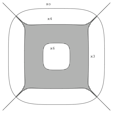
To determine the geometry more accurately, let us specialize to $(\eta_{1},\eta_{2},\eta_{3},$ $\eta_{4},\eta_{5})=(1,-1,-1,1,1)$. This seems to be the most interesting case which we were not able to solve by simpler methods. Inserting equations $(2^{\prime})$ and $(3^{\prime\prime})$ in equation $(1)$ we find

$$\textstyle{\frac{1}{2}}(\xi_{1}^{4}+\xi_{2}^{4}-r^{4})(\xi_{1}^{8}-\xi_{2}^{8})-{\frac{1}{2}}(\xi_{1}^{4}+\xi_{2}^{4})-2\xi_{3}^{4}+R^{4}+{\frac{1}{2}}r^{2}=0\,,$$

and the constraints become

$$(*)\quad \Rightarrow\qquad \xi_{1}^{4}+\xi_{2}^{4} \geq r^{4}\,,$$

$$(**)\quad \Rightarrow\qquad (\xi_{1}^{4}+\xi_{2}^{4}-r^{4})(\xi_{1}^{8}-\xi_{2}^{8})+(\xi_{1}^{4}+\xi_{2}^{4}) \leq 2R^{4}+r^{4}\,,$$

$$(*{*}*)\quad \Rightarrow\qquad (\xi_{1}^{4}+\xi_{2}^{4}-r^{4})(\xi_{1}^{8}-\xi_{2}^{8})-(\xi_{1}^{4}+\xi_{2}^{4}) \geq-2R^{4}-r^{4}\,.$$

The solution to those constraints is shown in figure 3. Patching the 4-fold cover together shows that $\Sigma$ is a 2-torus with four holes as depicted in figure 4. The circle is fibered over $\Sigma$ in the way described above.

Figure 4: $\Sigma$ is a 2-torus with four holes. The holes are shown as cuts. We also display representatives of homology 1-cycles.

The special lagrangian $M$ of interest now is the quotient of the circle fibration over $\Sigma$ by the residual ${\mathbb{Z}}_{2}\times{\mathbb{Z}}_{2}$ gauge symmetry. We want to understand the topology of this 3-manifold.

A.2 Topology

We can construct representatives of the homology cycles of $M$ by starting from the covering space, $\tilde{M}$, which is the trivial circle fibration over $\Sigma$. Since the fibers shrink to zero size at the boundaries of $\Sigma$ (denoted in figure 4 by the thick lines), there are no 1-cycles that reside in the fiber direction and therefore, using the Küneth formula, the 1-dimensional homology is determined by the 1-dimensional homology of the base. One possible choice of representatives of homology classes with orientations is shown in figure 4. Note, however, that the six cycles in figure 4 form an overcomplete basis of $H_{1}(S^{1}\rightarrow\Sigma)$ since they satisfy the relation

$$a+b+c+d=0\,.$$ (96)

Finding representatives of the homology classes of $M$ is simplified by that the ${\mathbb{Z}}_{2}\times{\mathbb{Z}}_{2}$ action has no fixed points. Therefore, all we have to do is to trace the original homology basis through the ${\mathbb{Z}}_{2}\times{\mathbb{Z}}_{2}$ projection and keep the invariant cycles.

By the charge table (23) in section 4.3.3, the first ${\mathbb{Z}}_{2}$ acts by $(-1,-1,1,1,1,1)$ on the six coordinates. This just halves the size of the $f$ cycle and identifies the cycles $a$ and $b$ with cycles $d$ and $c$, respectively. The second ${\mathbb{Z}}_{2}$ acts with charges $(1,1,-1,-1,-1,-1)$. Therefore, it will halve the size of the $e$ cycle, identify cycles $a$ and $d$ with $c$ and $b$, respectively, as well as shrink each circle fiber to half of its original size. Table 6 shows the action of the two ${\mathbb{Z}}_{2}$’s on the chosen (overcomplete) basis.

	$(-1,-1,1,1,1,1)$	$(1,1,-1,-1,-1,-1)$
$a$	$d$	$c$
$b$	$c$	$d$
$c$	$b$	$a$
$d$	$a$	$b$
$e$	$e+b+d$	$e$
$f$	$f$	$f+a+d$

Table 6: ${\mathbb{Z}}_{2}\times{\mathbb{Z}}_{2}$ action on the cohomology of $\tilde{M}$.

Since the two ${\mathbb{Z}}_{2}$ actions commute, they can be simultaneously diagonalized. Using the constraint equation (96), one shows that there are two homology classes that are invariant under the action of ${\mathbb{Z}}_{2}\times{\mathbb{Z}}_{2}$. Thus, $b_{0}(M)=1$ and $b_{1}(M)=2$. Furthermore, there is exactly one class in each non-trivial representation of ${\mathbb{Z}}_{2}\times{\mathbb{Z}}_{2}$. These results are summarized in table 7.

	$(-1,-1,1,1,1,1)=+1$	$(-1,-1,1,1,1,1)=-1$
$(1,1,-1,-1,-1,-1)=+1$	$\stackrel{{\scriptstyle\displaystyle{2f+a+d}}}{{\displaystyle{2e+b+d}}}$	$a-b+c-d$
$(1,1,-1,-1,-1,-1)=-1$	$a+d$	$a+b-c-d$

Table 7: Eigenvectors of the ${\mathbb{Z}}_{2}\times{\mathbb{Z}}_{2}$ action on the cohomology.

With these results in hand, we can now also compute the twisted (co)homology discussed in section 4. Recall that the real line bundle $L$ over $M$ is given by $L=\frac{\tilde{M}\times{\mathbb{R}}}{{\mathbb{Z}}_{2}\times{\mathbb{Z}}_{2}}$, where the ${\mathbb{Z}}_{2}\times{\mathbb{Z}}_{2}$ acts on the ${\mathbb{R}}$ fiber in a certain representation determined by the global B-field. The twisted cohomology is simply the ordinary cohomology of $\tilde{M}$ that is in the same representation as the fiber. Table 8 gives these Betti numbers for all possible twists.

			${\mathbb{Z}}_{2}\times{\mathbb{Z}}_{2}$ representation of fiber
			$(+,+)$		$(+,-)$		$(-,+)$		$(-,-)$
#($\eta_{1},\eta_{2}=-$)	#($\eta_{3},\eta_{4},\eta_{5}=-$)	$\tilde{M}$	$\hat{b}_{0}$	$\hat{b}_{1}$	$\hat{b}_{0}$	$\hat{b}_{1}$	$\hat{b}_{0}$	$\hat{b}_{1}$	$\hat{b}_{0}$	$\hat{b}_{1}$
0	0	$\emptyset$	0	0	0	0	0	0	0	0
0	1	$S^{1}\times S^{2}\times S^{0}$	1	1	1	1	0	0	0	0
0	2	$S^{1}\times S^{1}\times S^{1}$	1	3	0	0	0	0	0	0
0	3	$S^{1}\times S^{2}\times S^{0}$	1	1	1	1	0	0	0	0
1	0	$S^{3}\times S^{0}\times S^{0}$	1	0	1	0	1	0	1	0
1	1	$S^{1}$ over $\Sigma$	1	2	0	1	0	1	0	1

Table 8: The twisted Betti numbers of the fixed cycle in ${\mathbb{P}}_{11222}^{4}[8]$, depending on the $\eta_{i}$ and the ${\mathbb{Z}}_{2}\times{\mathbb{Z}}_{2}$ twist. The first ${\mathbb{Z}}_{2}$ acts only on $\xi_{1}$ and $\xi_{2}$, the second on $\xi_{3}$, $\xi_{4}$, $\xi_{5}$, and $\xi_{6}$.

The results of the LG phase are consistent with the spectra in the last two columns of this table, which is what appears in table 2.

Appendix B Chiral ${\mathbb{Z}}_{2}$ orbifolds

In this appendix, we summarize from refs. [73, 72] some generalities about ${\mathbb{Z}}_{2}$ orbifolds of rational conformal field theories originating from an order $2$ automorphism of the chiral algebra.
   Let ${\cal A}$ be a rational chiral algebra with irreducible representations $(R_{\lambda},{\cal H}_{\lambda})$ labelled by $\lambda\in\Lambda$. Let $\omega$ be an order $2$ automorphism of ${\cal A}$, and ${\cal A}^{\omega}$ the subalgebra of ${\cal A}$ that is left pointwise fixed under $\omega$.
   By definition, for every representation $R_{\lambda}$, $R_{\lambda}{\circ}\omega$ is again a representation of ${\cal A}$. In this way, $\omega$ induces an action on the set of irreducible representations, $\omega^{*}:\Lambda\to\Lambda$. Assume that $\omega$ can be implemented as a twisted intertwiner on the representation spaces, i.e.,

$${\cal T}^{\omega}:{\cal H}_{\lambda}\to{\cal H}_{\omega^{*}\lambda}\text{\; such that for all $a\in{\cal A}$,\; }{\cal T}^{\omega}{\circ}R_{\lambda}(\omega(a))=R_{\omega^{*}\lambda}(a){\circ}{\cal T}^{\omega}\,.$$ (97)

   Any irreducible representation $\lambda$ of ${\cal A}$ induces by restriction a representation of ${\cal A}^{\omega}$. This representation is irreducible precisely if $\omega^{*}\lambda\neq\lambda$ (non-symmetric representation). The representations induced from $(R_{\lambda},{\cal H}_{\lambda})$ and $(R_{\omega^{*}\lambda},{\cal H}_{\omega^{*}\lambda})$ then become isomorphic and give rise to one irreducible representation of ${\cal A}^{\omega}$. If, on the other hand, $\omega^{*}\lambda=\lambda$ (symmetric representation), then the induced representation is reducible (and fully reducible) as a representation of ${\cal A}^{\omega}$, and gives rise to two irreducible representations of ${\cal A}^{\omega}$. Those irreducible representations which are induced from representations of ${\cal A}$ are said to be “in the untwisted sector”.
   There are furthermore irreducible representations which are not induced from those of ${\cal A}$. They are said to be “in the twisted sector”.
   To summarize, there are three different kinds of irreducible representations of ${\cal A}^{\omega}$. Untwisted representations inherit their labels from ${\cal A}$. If they come from non-symmetric representations, we shall denote them by ${}^{\rm un}\lambda\equiv{}^{\rm un}(\omega^{*}\lambda)$. The two irreducible representations that come from symmetric representations of ${\cal A}$ will be distinghuished by labels ${}^{\rm us}\lambda{}_{{}^{+}}$ and ${}^{\rm us}\lambda{}_{{}^{-}}$. Finally, twisted representations require new labels, of the generic form ${}^{\rm tw}\dot{\lambda}\psi$, with $\psi=\pm$.
   According to [72, 73], the full modular data of the orbifold can be determined from the so-called twining characters. Formally, these are defined for every symmetric representation $\lambda$ by the formula

$$\chi^{(0)}_{\lambda}(2\tau)={\rm tr}_{{\cal H}_{\lambda}}{\cal T}^{\omega}q^{L_{0}-c/24}\,,$$ (98)

where, as usual, $q={\rm e}^{2\pi{\rm i}\tau}$, and ${\cal T}^{\omega}:{\cal H}_{\lambda}\to{\cal H}_{\lambda}$ is as in eq. (97).
   The characters of the orbifold theory in the untwisted sector are then given by

$$\chi^{\cal O}_{{}^{\rm un}\lambda}(\tau) =\chi_{\lambda}(\tau)$$ (99)

$$\chi^{\cal O}_{{}^{\rm us}\lambda\psi}(\tau) =\frac{1}{2}\bigl{(}\chi_{\lambda}(\tau)+\psi\,\eta_{\lambda}^{-1}\,\chi^{(0)}_{\lambda}(2\tau)\bigr{)}\,.$$ (100)

Here, $\eta_{\lambda}$ is a certain conventional phase, which is determined by the conjugation properties of the representation $\lambda$.
   Under modular transformation, the characters in (99) and (100) do not close onto themselves, but rather lead to the characters in the twisted sectors. Namely, for every twisted sector $\dot{\lambda}$, there is a function $\chi^{(1)}_{\dot{\lambda}}(\tau)$ such that the characters of the two twisted representations are given by

$$\chi^{\cal O}_{{}^{\rm tw}\dot{\lambda}\psi}(\tau)=\frac{1}{2}\Bigl{(}\chi^{(1)}_{\dot{\lambda}}(\frac{\tau}{2})+\psi\,\bigl{(}T_{\dot{\lambda}}^{(1)}\bigr{)}^{-1/2}\,\chi^{(1)}_{\dot{\lambda}}\bigl{(}\frac{\tau+1}{2}\bigr{)}\Bigr{)}\,.$$ (101)

Here, $T_{\dot{\lambda}}^{(1)}$ is part of (the square of) the modular T-matrix and determines the conformal weights in the twisted sectors up to (half) integers.
   The relevant modular-S transformations are

$$\chi^{(0)}_{\lambda}\bigl{(}-\frac{1}{\tau}\bigr{)} =\sum_{\dot{\mu}}S^{(0)}_{\lambda,\dot{\mu}}\chi^{(1)}_{\dot{\mu}}(\tau)$$ (102)

and

$$\chi^{(1)}_{\dot{\lambda}}\bigl{(}-\frac{1}{\tau}\bigr{)} =\sum_{\mu}S_{\dot{\lambda},\mu}^{(1)}\chi^{(0)}_{\mu}(\tau)\,,$$ (103)

where the matrices $S^{(0)}$ and $S^{(1)}$ are square, non-singular, and related to each other by phases.
   We now collect from [73] the formulae for the modular S-matrix, $S^{\cal O}$, of the orbifold. Matrix elements of $S^{\cal O}$ between only untwisted representations depend only on the S-matrix of the parent theory,

$$S^{\cal O}_{{}^{\rm un}\lambda,{}^{\rm un}\mu} =S_{\lambda,\mu}+S_{\lambda,\omega^{*}\mu}$$

$$S^{\cal O}_{{}^{\rm un}\lambda,{}^{\rm us}\mu\psi} =S_{\lambda,\mu}$$ (104)

$$S^{\cal O}_{{}^{\rm us}\lambda\psi,{}^{\rm us}\mu\psi^{\prime}} =\frac{1}{2}S_{\lambda,\mu}\,.$$

Matrix elements between untwisted and twisted representations involve, of course, $$S^{(0)} S^{(1)}$$ and ,

$$S^{\cal O}_{{}^{\rm un}\lambda,{}^{\rm tw}\dot{\mu}\psi} =0$$

$$S^{\cal O}_{{}^{\rm us}\lambda\psi,{}^{\rm tw}\dot{\mu}\psi} =\frac{1}{2}\psi\eta_{\lambda}^{-1}S^{(0)}_{\lambda,\dot{\mu}}=\frac{1}{2}\psi\eta_{\lambda}S^{(1)}_{\dot{\mu},\lambda}$$ (105)

Finally, matrix elements between twisted representations are given by

$$S_{{}^{\rm tw}\dot{\lambda}\psi,{}^{\rm tw}\dot{\mu}\psi^{\prime}} =\frac{1}{2}\psi\psi^{\prime}P_{\dot{\lambda},\dot{\mu}}\,,$$ (106)

where $P$ is the matrix

$$P=\bigl{(}T^{(1)}\bigr{)}^{1/2}S^{(1)}\bigl{(}T^{(0)}\bigr{)}^{2}S^{(0)}\bigl{(}T^{(1)}\bigr{)}^{1/2}\,.$$ (107)

Appendix C ${\mathbb{Z}}_{2}$ orbifolds of SU$(2)_{k}$ and U$(1)_{2N}$

We here record for reference the modular data of the ${\mathbb{Z}}_{2}$ orbifolds of SU$(2)$ WZW models and of the compactified free boson.

C.1 SU$(2)$ WZW

The modular data of the orbifold of the SU$(2)$ WZW model at level $k$ by charge conjugation can easily be extracted from [73]. Note that since charge conjugation is an inner automorphism for SU$(2)$, all primaries are symmetric (i.e., self-conjugate). As in the main text, we distinguish untwisted (symmetric) and twisted sectors by adding a prefix ^us and ^tw, respectively. The list of primary fields of the orbifold then is as follows.

sector	labels and range		conformal weight
untwisted
	${}^{\rm us}l\psi$	$l=0,\ldots,k$	$\frac{l(l+2)}{4h}$    (but $\Delta_{{}^{\rm us}0{}_{{}^{+}}}=1$)
twisted
	${}^{\rm tw}\lambda\psi$	$\lambda=0,\ldots,k$	$\frac{c}{24}+\frac{(k-2\lambda)^{2}}{16h}+\frac{1}{4}(1-\epsilon_{\lambda}\psi)$

Here, $c=3k/h$ is the central charge and $h=k+2$. In the twisted sector, the conformal weights of the two primaries with given $\lambda$ differ by $\frac{1}{2}$, but the choice $\epsilon_{\lambda}=\pm 1$ is arbitrary. The choices of [73] amount to $\epsilon_{\lambda}=(-1)^{\lambda}$. This is also the assignement used in the main text.

The modular S-matrix is given by the formulae

$$\begin{split}S_{{}^{\rm us}l\psi,{}^{\rm us}l^{\prime}\psi^{\prime}}&=\frac{1}{\sqrt{2(k+2)}}\,\sin\pi\frac{(l+1)(l^{\prime}+1)}{k+2}\\ S_{{}^{\rm us}l\psi,{}^{\rm tw}\lambda\psi^{\prime}}&=\frac{\psi\,{\rm i}^{-l}}{\sqrt{2(k+2)}}\,\sin\pi\frac{(l+1)(\lambda+1)}{k+2}\\ S_{{}^{\rm tw}\lambda\psi,{}^{\rm tw}\lambda^{\prime}\psi^{\prime}}&=\frac{\psi\psi^{\prime}\,{\rm i}^{-\lambda-\lambda^{\prime}}\,{\rm e}^{-2\pi{\rm i}k/8}}{\sqrt{2(k+2)}}\,\sin\pi\frac{(\lambda+1)(\lambda^{\prime}+1)}{k+2}\,.\end{split}$$ (108)

C.2 Compactified free boson

Consider the free boson CFT and its ${\mathbb{Z}}_{2}$ orbifold by the charge conjugation automorphism (see, for instance, [95]). If the boson is compactified on a circle with rational radius squared, the (extended) chiral algebra of the model becomes rational. In this case, the finite number, $2N$, of primary fields of the non-orbifolded theory are labelled by the U$(1)$ charge, $k=0,\ldots,2N-1\bmod 2N$. Charge conjugation acts on the U$(1)$ current as $J\mapsto-J$. The action on primary fields is $k\mapsto-k$, so that there are two symmetric sectors, $k=0$ and $k=N$. Accordingly, there are two twisted sectors, with two primary fields each. Altogether, the orbifold has the following $N+7$ primary fields.

sector		labels and range		conformal weight
untwisted
	non-symmetric	${}^{\rm un}k$	$k=1,\ldots N-1$	$k^{2}/4N$
	symmetric	${}^{\rm us}k\psi$	$k=0,N$; $\psi=\pm$	$\Delta_{0{}_{{}^{+}}}=0$; $\Delta_{0{}_{{}^{-}}}=1$ $\Delta_{N{}_{{}^{+}}}=\Delta_{N{}_{{}^{-}}}=N/4$
twisted
		${}^{\rm tw}\sigma\psi$	$\sigma=0,1$; $\psi=\pm$	$\frac{1}{16}+\frac{1}{4}(1-\psi(-1)^{N\sigma})$

(The conventional notation [95] in the twisted sector is $\sigma_{1,2}$ for the twist fields with $\Delta=\frac{1}{16}$ and $\tau_{1,2}$ for those with $\Delta=\frac{9}{16}$.)

The corresponding characters and their modular transformation properties can be found in [72]. However, as is often the case in similar situations, some of the characters coincide, and hence this does not fully determine the modular S-matrix. There are two more constraints that can be used to fix the resulting ambiguity: the relation $(ST)^{3}=S^{2}$ between modular S- and T-matrices and integrality of fusion rules. It turns out that the S-matrices given in [72] do not quite satisfy the relation $(ST)^{3}=S^{2}$ in the modular group. More precisely, the S-matrix entries involving twisted sectors actually depend on $N\bmod 4$, and not ${}\bmod 2$, as shown in [72]. But the fusion rules computed in [72] are integral, and indeed coincide with the ones computed from (109). The full S-matrix is given by

$$\begin{split}S_{{}^{\rm un}k,{}^{\rm un}k^{\prime}}&=\sqrt{\frac{2}{N}}\,\cos\pi\frac{kk^{\prime}}{N}\\ S_{{}^{\rm us}k\psi,{}^{\rm un}k^{\prime}}&=\frac{1}{\sqrt{2N}}\,{\rm e}^{-\pi{\rm i}kk^{\prime}/N}\\ S_{{}^{\rm us}k\psi,{}^{\rm us}k^{\prime}\psi^{\prime}}&=\frac{1}{\sqrt{8N}}\,{\rm e}^{-\pi{\rm i}kk^{\prime}/N}\\ S_{{}^{\rm un}k,{}^{\rm tw}\sigma\psi}&=0\\ S_{{}^{\rm us}k\psi,{}^{\rm tw}\sigma\psi^{\prime}}&=\frac{\psi}{\sqrt{8}}\begin{pmatrix}1&1\\ {\rm i}^{-N}&-{\rm i}^{-N}\end{pmatrix}\\ S_{{}^{\rm tw}\sigma\psi,{}^{\rm tw}\sigma^{\prime}\psi^{\prime}}&=\frac{\psi\psi^{\prime}}{4}\begin{pmatrix}\;\;\;\;1\,+{\rm i}^{-N}&(-1)^{N}-{\rm i}^{N}\\ (-1)^{N}-{\rm i}^{N}&\;\;\;\;1\,+{\rm i}^{-N}\end{pmatrix}\,,\end{split}$$ (109)

where rows and columns in the last two lines are indexed by $k=0,N$ and $\sigma,\sigma^{\prime}=0,1$, respectively.

References

- [1] S. L. Shatashvili and C. Vafa, “Superstrings and manifold of exceptional holonomy,” hep-th/9407025.
- [2] J. M. Figueroa-O’Farrill, “A note on the extended superconformal algebras associated with manifolds of exceptional holonomy,” Phys. Lett. B392 (1997) 77–84, hep-th/9609113.
- [3] G. Papadopoulos and P. K. Townsend, “Compactification of D = 11 supergravity on spaces of exceptional holonomy,” Phys. Lett. B357 (1995) 300–306, hep-th/9506150.
- [4] B. S. Acharya, “M theory, Joyce orbifolds and super Yang-Mills,” Adv. Theor. Math. Phys. 3 (1999) 227–248, hep-th/9812205.
- [5] B. S. Acharya, “On realising N = 1 super Yang-Mills in M theory,” hep-th/0011089.
- [6] M. Atiyah, J. Maldacena, and C. Vafa, “An M-theory flop as a large N duality,” J. Math. Phys. 42 (2001) 3209–3220, hep-th/0011256.
- [7] M. Cvetic, G. Shiu, and A. M. Uranga, “Three-family supersymmetric standard like models from intersecting brane worlds,” Phys. Rev. Lett. 87 (2001) 201801, hep-th/0107143.
- [8] M. Cvetic, G. Shiu, and A. M. Uranga, “Chiral four-dimensional N = 1 supersymmetric type IIA orientifolds from intersecting D6-branes,” Nucl. Phys. B615 (2001) 3–32, hep-th/0107166.
- [9] M. Atiyah and E. Witten, “M-theory dynamics on a manifold of G(2) holonomy,” hep-th/0107177.
- [10] E. Witten, “Anomaly cancellation on G(2) manifolds,” hep-th/0108165.
- [11] B. Acharya and E. Witten, “Chiral fermions from manifolds of G(2) holonomy,” hep-th/0109152.
- [12] H. Partouche and B. Pioline, “Rolling among G(2) vacua,” JHEP 03 (2001) 005, hep-th/0011130.
- [13] P. Kaste, A. Kehagias, and H. Partouche, “Phases of supersymmetric gauge theories from M-theory on G(2) manifolds,” JHEP 05 (2001) 058, hep-th/0104124.
- [14] A. Giveon, A. Kehagias, and H. Partouche, “Geometric transitions, brane dynamics and gauge theories,” hep-th/0110115.
- [15] M. Cvetic, G. W. Gibbons, H. Lu, and C. N. Pope, “New complete non-compact Spin(7) manifolds,” Nucl. Phys. B620 (2002) 29–54, hep-th/0103155.
- [16] M. Cvetic, G. W. Gibbons, H. Lu, and C. N. Pope, “Supersymmetry M3-branes and G(2) manifolds,” Nucl. Phys. B620 (2002) 3–28, hep-th/0106026.
- [17] A. Brandhuber, J. Gomis, S. S. Gubser, and S. Gukov, “Gauge theory at large N and new G(2) holonomy metrics,” Nucl. Phys. B611 (2001) 179–204, hep-th/0106034.
- [18] M. Cvetic, G. W. Gibbons, H. Lu, and C. N. Pope, “M-theory conifolds,” Phys. Rev. Lett. 88 (2002) 121602, hep-th/0112098.
- [19] A. Brandhuber, “G(2) holonomy spaces from invariant three-forms,” hep-th/0112113.
- [20] M. Cvetic, G. W. Gibbons, H. Lu, and C. N. Pope, “A G(2) unification of the deformed and resolved conifolds,” hep-th/0112138.
- [21] E. Witten, “Deconstruction, G(2) holonomy, and doublet-triplet splitting,” hep-ph/0201018.
- [22] H. Ita, Y. Oz, and T. Sakai, “Comments on M theory dynamics on G(2) holonomy manifolds,” hep-th/0203052.
- [23] T. Friedmann, “On the quantum moduli space of M theory compactifications,” hep-th/0203256.
- [24] T. Eguchi and Y. Sugawara, “CFT description of string theory compactified on non- compact manifolds with G(2) holonomy,” Phys. Lett. B519 (2001) 149–158, hep-th/0108091.
- [25] K. Sugiyama and S. Yamaguchi, “Cascade of special holonomy manifolds and heterotic string theory,” Nucl. Phys. B622 (2002) 3–45, hep-th/0108219.
- [26] R. Blumenhagen and V. Braun, “Superconformal field theories for compact G(2) manifolds,” JHEP 12 (2001) 006, hep-th/0110232.
- [27] R. Roiban and J. Walcher, “Rational conformal field theories with G(2) holonomy,” JHEP 12 (2001) 008, hep-th/0110302.
- [28] T. Eguchi and Y. Sugawara, “String theory on G(2) manifolds based on Gepner construction,” hep-th/0111012.
- [29] R. Blumenhagen and V. Braun, “Superconformal field theories for compact manifolds with Spin(7) holonomy,” JHEP 12 (2001) 013, hep-th/0111048.
- [30] B. R. Greene, C. Vafa, and N. P. Warner, “Calabi-Yau manifolds and renormalization group flows,” Nucl. Phys. B324 (1989) 371.
- [31] C. Vafa and N. P. Warner, “Catastrophes and the classification of conformal theories,” Phys. Lett. B218 (1989) 51.
- [32] W. Lerche, C. Vafa, and N. P. Warner, “Chiral rings in N=2 superconformal theories,” Nucl. Phys. B324 (1989) 427.
- [33] C. Vafa, “String vacua and orbifoldized L-G models,” Mod. Phys. Lett. A4 (1989) 1169.
- [34] E. Witten, “Phases of N = 2 theories in two dimensions,” Nucl. Phys. B403 (1993) 159–222, hep-th/9301042.
- [35] D. Gepner, “Exactly solvable string compactifications on manifolds of SU(N) holonomy,” Phys. Lett. B199 (1987) 380–388.
- [36] D. Gepner, “Space-time supersymmetry in compactified string theory and superconformal models,” Nucl. Phys. B296 (1988) 757.
- [37] L. J. Dixon, “Some world-sheet properties of superstring compactifications, on orbifolds and otherwise,” in Superstrings, unified theories and cosmology 1987 (Trieste, 1987), pp. 67–126. World Sci. Publishing, Teaneck, NJ, 1988.
- [38] S. Katz, D. R. Morrison, and M. Ronen Plesser, “Enhanced Gauge Symmetry in Type II String Theory,” Nucl. Phys. B477 (1996) 105–140, hep-th/9601108.
- [39] S. Katz, A. Klemm, and C. Vafa, “Geometric engineering of quantum field theories,” Nucl. Phys. B497 (1997) 173–195, hep-th/9609239.
- [40] S. Katz, P. Mayr, and C. Vafa, “Mirror symmetry and exact solution of 4D N = 2 gauge theories. I,” Adv. Theor. Math. Phys. 1 (1998) 53–114, hep-th/9706110.
- [41] P. S. Aspinwall, “Enhanced gauge symmetries and K3 surfaces,” Phys. Lett. B357 (1995) 329–334, hep-th/9507012.
- [42] M. Bershadsky, C. Vafa, and V. Sadov, “D-Branes and Topological Field Theories,” Nucl. Phys. B463 (1996) 420–434, hep-th/9511222.
- [43] C. Vafa, “Modular invariance and discrete torsion on orbifolds,” Nucl. Phys. B273 (1986) 592.
- [44] E. R. Sharpe, “Discrete torsion and gerbes. I,” hep-th/9909108.
- [45] E. R. Sharpe, “Discrete torsion and gerbes. II,” hep-th/9909120.
- [46] E. R. Sharpe, “Discrete torsion,” hep-th/0008154.
- [47] R. L. Bryant and S. M. Salamon, “On the construction of some complete metrics with exceptional holonomy,” Duke Math. J. 58 (1989), no. 3, 829–850.
- [48] G. W. Gibbons, D. N. Page, and C. N. Pope, “Einstein metrics on S**3 R**3 and R**4 bundles,” Commun. Math. Phys. 127 (1990) 529.
- [49] D. D. Joyce, Compact manifolds with special holonomy. Oxford University Press, Oxford, 2000.
- [50] R. C. Mc Lean, Deformations and Moduli of Calibrated Submanifolds. PhD thesis, Duke University, 1990.
- [51] K. A. Intriligator and N. Seiberg, “Mirror symmetry in three dimensional gauge theories,” Phys. Lett. B387 (1996) 513–519, hep-th/9607207.
- [52] J. de Boer, K. Hori, H. Ooguri, and Y. Oz, “Mirror symmetry in three-dimensional gauge theories, quivers and D-branes,” Nucl. Phys. B493 (1997) 101–147, hep-th/9611063.
- [53] G. Ferretti, P. Salomonson, and D. Tsimpis, “D-brane probes on G(2) orbifolds,” JHEP 03 (2002) 004, hep-th/0111050.
- [54] S. Gukov and D. Tong, “D-brane probes of special holonomy manifolds, and dynamics of N = 1 three-dimensional gauge theories,” hep-th/0202126.
- [55] B. S. Acharya, “On mirror symmetry for manifolds of exceptional holonomy,” Nucl. Phys. B524 (1998) 269–282, hep-th/9707186.
- [56] M. Aganagic and C. Vafa, “G(2) manifolds, mirror symmetry and geometric engineering,” hep-th/0110171.
- [57] S. Gukov, S.-T. Yau, and E. Zaslow, “Duality and fibrations on G(2) manifolds,” hep-th/0203217.
- [58] E. Witten, “D-branes and K-theory,” JHEP 12 (1998) 019, hep-th/9810188.
- [59] E. Witten, “Toroidal compactification without vector structure,” JHEP 02 (1998) 006, hep-th/9712028.
- [60] E. Witten, “Phase Transitions In M-Theory And F-Theory,” Nucl. Phys. B471 (1996) 195–216, hep-th/9603150.
- [61] E. Witten, “New issues in manifolds of SU(3) holonomy,” Nucl. Phys. B268 (1986) 79.
- [62] E. Witten, “Dyons Of Charge ,” Phys. Lett. B86 (1979) 283–287.
- [63] K. Becker, M. Becker, and A. Strominger, “Five-branes, membranes and nonperturbative string theory,” Nucl. Phys. B456 (1995) 130–152, hep-th/9507158.
- [64] I. Brunner, M. R. Douglas, A. Lawrence, and C. Römelsberger, “D-branes on the quintic,” JHEP 08 (2000) 015, hep-th/9906200.
- [65] A. B. Zamolodchikov and V. A. Fateev, “Disorder fields in two-dimensional conformal quantum field theory and N=2 extended supersymmetry,” Sov. Phys. JETP 63 (1986) 913–919.
- [66] Z.-A. Qiu, “Conformal field theories and modular invariant partition functions for parafermion field theories,” Nucl. Phys. B295 (1988) 171.
- [67] F. Ravanini and S.-K. Yang, “C disorder fields and twist partition functions in parafermionic conformal field theories,” Nucl. Phys. B295 (1988) 262.
- [68] A. Recknagel and V. Schomerus, “D-branes in Gepner models,” Nucl. Phys. B531 (1998) 185–225, hep-th/9712186.
- [69] J. Fuchs, P. Kaste, W. Lerche, C. A. Lütken, C. Schweigert, and J. Walcher, “Boundary fixed points, enhanced gauge symmetry and singular bundles on K3,” Nucl. Phys. B598 (2001) 57–72, hep-th/0007145.
- [70] J. Maldacena, G. W. Moore, and N. Seiberg, “Geometrical interpretation of D-branes in gauged WZW models,” JHEP 07 (2001) 046, hep-th/0105038.
- [71] B. R. Greene and M. R. Plesser, “Duality in Calabi-Yau moduli space,” Nucl. Phys. B338 (1990) 15–37.
- [72] R. Dijkgraaf, C. Vafa, E. Verlinde, and H. Verlinde, “The operator algebra of orbifold models,” Commun. Math. Phys. 123 (1989) 485.
- [73] L. Birke, J. Fuchs, and C. Schweigert, “Symmetry breaking boundary conditions and WZW orbifolds,” hep-th/9905038.
- [74] D. Gepner and B. Noyvert, “Unitary representations of SW(3/2,2) superconformal algebra,” Nucl. Phys. B610 (2001) 545–577, hep-th/0101116.
- [75] B. Noyvert, “Unitary minimal models of SW(3/2,3/2,2) superconformal algebra and manifolds of G(2) holonomy,” hep-th/0201198.
- [76] A. N. Schellekens and S. Yankielowicz, “Simple currents, modular invariants and fixed points,” Int. J. Mod. Phys. A5 (1990) 2903–2952.
- [77] J. Fuchs, A. N. Schellekens, and C. Schweigert, “A matrix S for all simple current extensions,” Nucl. Phys. B473 (1996) 323–366, hep-th/9601078.
- [78] J. L. Cardy, “Boundary conditions, fusion rules and the Verlinde formula,” Nucl. Phys. B324 (1989) 581.
- [79] J. Fuchs and C. Schweigert, “Symmetry breaking boundaries. I: General theory,” Nucl. Phys. B558 (1999) 419–483, hep-th/9902132.
- [80] J. Fuchs, L. R. Huiszoon, A. N. Schellekens, C. Schweigert, and J. Walcher, “Boundaries, crosscaps and simple currents,” Phys. Lett. B495 (2000) 427–434, hep-th/0007174.
- [81] I. Brunner and V. Schomerus, “D-branes at singular curves of Calabi-Yau compactifications,” JHEP 04 (2000) 020, hep-th/0001132.
- [82] Z.-A. Qiu, “Modular invariant partition functions for N=2 superconformal field theories,” Phys. Lett. B198 (1987) 497.
- [83] F. Ravanini and S.-K. Yang, “Modular invariance in N=2 superconformal field theories,” Phys. Lett. B195 (1987) 202.
- [84] A. Cappelli, C. Itzykson, and J. B. Zuber, “Modular invariant partition functions in two-dimensions,” Nucl. Phys. B280 (1987) 445–465.
- [85] A. Cappelli, C. Itzykson, and J. B. Zuber, “The ADE classification of minimal and A1(1) conformal invariant theories,” Commun. Math. Phys. 113 (1987) 1.
- [86] W. Lerche, “On a boundary CFT description of nonperturbative N = 2 Yang-Mills theory,” hep-th/0006100.
- [87] W. Lerche, C. A. Lütken, and C. Schweigert, “D-branes on ALE spaces and the ADE classification of conformal field theories,” hep-th/0006247.
- [88] V. I. Arnol′d, S. M. Guseĭn-Zade, and A. N. Varchenko, Singularities of differentiable maps. Vol. I. Birkhäuser Boston Inc., Boston, MA, 1985. The classification of critical points, caustics and wave fronts, Translated from the Russian by Ian Porteous and Mark Reynolds.
- [89] D. A. Kastor, E. J. Martinec, and S. H. Shenker, “RG flow in N=1 discrete series,” Nucl. Phys. B316 (1989) 590–608.
- [90] A. B. Zamolodchikov, “Conformal symmetry and multicritical points in two- dimensional quantum field theory.,” Sov. J. Nucl. Phys. 44 (1986) 529–533.
- [91] A. Cappelli, “Modular invariant partition functions of superconformal theories,” Phys. Lett. B185 (1987) 82–88.
- [92] L. J. Dixon, J. A. Harvey, C. Vafa, and E. Witten, “Strings on orbifolds,” Nucl. Phys. B261 (1985) 678–686.
- [93] T. Gannon, “U(1)**m modular invariants, N = 2 minimal models, and the quantum Hall effect,” Nucl. Phys. B491 (1997) 659–688, hep-th/9608063.
- [94] E. Witten, “Constraints on supersymmetry breaking,” Nucl. Phys. B202 (1982) 253.
- [95] P. Ginsparg, “Applied conformal field theory,”. Lectures given at Les Houches Summer School in Theoretical Physics, Les Houches, France, Jun 28 - Aug 5, 1988.
- [96] E. Witten, “Supersymmetry and Morse theory,” J. Diff. Geom. 17 (1982) 661–692.
- [97] M. R. Douglas, “D-branes, categories and N = 1 supersymmetry,” hep-th/0011017.
- [98] N. C. Leung and C. Vafa, “Branes and toric geometry,” Adv. Theor. Math. Phys. 2 (1998) 91–118, hep-th/9711013.
- [99] K. Hori, A. Iqbal, and C. Vafa, “D-branes and mirror symmetry,” hep-th/0005247.
- [100] M. Aganagic and C. Vafa, “Mirror symmetry, D-branes and counting holomorphic discs,” hep-th/0012041.