Comparing Implicit, Differential, Dimensional and BPHZ Renormalisation

We compare a momentum space implicit regularisation (IR) framework with other renormalisation methods which may be applied to dimension specific theories, namely Differential Renormalisation (DfR) and the BPHZ formalism. In particular, we define what is meant by minimal subtraction in IR in connection with DfR and dimensional renormalisation (DR) . We illustrate with the calculation of the gluon self energy a procedure by which a constrained version of IR automatically ensures gauge invariance at one loop level and handles infrared divergences in a straightforward fashion. Moreover, using the $\varphi^{4}_{4}$ theory setting sun diagram as an example and comparing explicitly with the BPHZ framework, we show that IR directly displays the finite part of the amplitudes. We then construct a parametrization for the ambiguity in separating the infinite and finite parts whose parameter serves as renormalisation group scale for the Callan-Symanzik equation. Finally we argue that constrained IR, constrained DfR and dimensional reduction are equivalent within one loop order.

Pacs:11.10.Gh, 11.25.Db, 11.15.Bt.
Keywords: Regularisation methods, Dimension Specific

1 Introduction

It is well known that the higher the symmetry degree of a quantum field theoretic model the more stringent are the constraints on a consistent regularisation scheme to handle the divergences which appear in diagrammatic expansions. For example, whereas a sharp cutoff may be successfully employed in most scalar field theories to reflect the correct physics in perturbation theory, it does not work so well already for abelian gauge field theories. For gauge field theories, DR is one of the most suitable frameworks because the amplitudes can be renormalised using for instance a minimal subtraction scheme (MS) and readily satisfy the Slavnov-Taylor identities.

However some symmetries which are present in the integer dimension may not have a direct analogue in $n$ dimensions. This is the case of supersymmetric (SUSY), chiral and topological field theories (the so called dimension specific theories). Some modifications of DR can be effected in order to mend certain shortcomings. For instance one may construct an extension of the algebra of the $\gamma^{5}$ matrix to dimension $n$ and control eventual spurious anomalies by imposing the Slavnov-Taylor identities as constraint equations. This is the usual procedure in the Electroweak Sector of the Standard Model. In Chern-Simons theories it may be necessary to employ an hybrid regularisation procedure by adding Higher Covariant Derivative terms in the Lagrangian which improves the ultraviolet behaviour. The remaining divergences are dealt with DR and adopting an extension of the Levi-Civitta tensor algebra to be compatible with analytical continuation on the space-time dimension. The main drawback in the example above is that the calculation may become extremely complicated beyond the one loop order. A variant of DR called Dimensional Reduction (DRed) was proposed by Siegel [1]. The latter differs from DR in the sense that the continuation from $4$ to $n$ dimensions is made by compactification. Thus whereas the momentum (or space-time) integrals are $n$-dimensional, the number of field components remains unchanged. Such procedure, however, may introduce ambiguities in the finite parts of the amplitudes as well as in the divergent parts in high order corrections. DRed has been largely employed especially in supersymmetric models as the invariance of the action with respect to SUSY transformations holds in general only for specific values of $n$. Unfortunately DRed appears to work well only at one loop level. In fact, DRed can be shown to be inconsistent in general with analytical continuation [2], [3] when $\gamma_{5}$ matrices and $\epsilon_{\mu_{1}\mu_{2}\ldots}$ tensors are considered. In general a pragmatic attitude is adopted in handling the shortcomings brought by flawed regularisation frameworks especially when the model in consideration is known to be free of anomalies. In other words the task of treating the infinities in diagrammatic calculations, especially for theories which are sensitive to dimensional continuation, without introducing ambiguities steming from the regulator employed (that is to say, a regulator independent method) is still a subject of major interest. Ultimately it is desirable to construct a framework in which one has simultaneously : 1) no need to add structure to the Lagrangian and hence complicate the Feynman rules; 2) (nonabelian) gauge invariance is systematically guaranteed without having to be imposed as constraint equations order by order; 3) control upon infrared divergences without introducing additional machinery and 4) a method that is friendly from the calculational viewpoint.

The task of treating the ultraviolet infinities in a regulator free fashion has been firstly conceived within the BPHZ formalism [4]. This framework relies ultimately in Weinberg’s theorem which states that a Feynman graph converges if the degree of divergence of the graph and all its subgraphs is negative. A systematic implementation of this idea is the Dyson’s scheme which is based on the idea that differentiation with respect to the external momentum turns the graph less divergent. Hence in Dyson’s method the divergent parts of a graph $G$ are subtracted by applying Taylor operators $t^{d(\gamma)}$ where $d(\gamma)$ is the degree of superficial divergence starting from the smallest subgraphs. When overlapping divergences occur care must be exercised in such subtraction procedure. The BPHZ framework is the generalisation of the Dyson procedure to include overlapping diagrams by means of a well prescribed formula called the forest formula. Although BPHZ is a very powerful framework which enables to construct proofs of renormalizability to all orders, gauge invariance and hence the Slavnov Taylor identities should be imposed as constraint equations. The reason why gauge invariance is broken when the BPHZ method is applied to nonabelian gauge theories lies in the subtraction process which is based on expanding around an external momentum and thus modifying the structure of the corresponding amplitude. Some modifications in the BPHZ framework (Soft BPHZ Scheme) must be made to handle infrared divergencies because in the original formulation the subtraction is constructed at zero external momentum [5].

DfR [7]-[16] and IR (please see [17]-[23] for applications) seem to be very promising in this sense since they do not modify the space time dimension or introduce an explicit regulator at any step of the calculation. The former is position space method (contact with momentum space is made by means of Fourier transforms) whereas the latter is essentially constructed in momentum space. We shall discuss these methods in greater detail throughout this paper. We believe that the comparison which we shall outline here will show that IR is a promising candidate for handling divergences in field theoretical calculations (UV and infrared) in general in a symmetry preserving fashion yet being simple from the computational point of view.

This paper is organized as follows: in section 1) we give a brief description of DfR and IR and compare with DR. We work out a few examples in $\phi^{4}$ theory and $QED$ where we discuss the role played by momentum routing invariance in connection with gauge invariance to effect a constrained version of IR. We also claim that to one loop order dimensional Reduction, DfR and IR are equivalent and define what is meant by minimal subtraction in IR. In section 2) we compute explicitly the setting sun diagram in both BPHZ, IR and compare with DfR. This is a nontrivial example because it possesses an interesting divergent structure from which we will clearly see the advantages of applying IR and DfR especially in obtaining the finite part. In section 3) we calculate the gluon self energy in $QCD$ within IR to show that it can consistently handle the infrared divergences as well as readily display the finite part expressed by a class of well defined functions. We conclude by outlining a few applications in which IR could be useful and perhaps more advantageous.

2 Relationship between Differential, Implicit and Dimensional Renormalisation

DfR was introduced by Freedman, Johnson and Latorre [7] as a method of regularization and renormalization in coordinate (Euclidian) space. The idea is that the product of propagators is not a distribution and so it has no Fourier transform. In DfR, renormalization is the procedure which extend products of distributions into distributions by substituting bad-behaved expressions by derivatives of well-behaved ones [8] which are understood as distributions, that is to say, the derivatives are meant to act on test functions. It automatically delivers finite Green’s functions (which are identical to the bare ones for separate points but behave well enough at coincident points) without introducing an intermediate regulator or counterterm. For instance, suppose that we have¡B¿¡/B¿ an amplitude proportional to the product of massless propagators

$$\Delta_{0}(x)=\frac{1}{4\pi^{2}x^{2}}\,\,\,,x^{2}=x_{\mu}x_{\mu}.$$ (1)

Although $(\ref{eq:mlprop})$ is a well defined distribution its square is not. According to DfR we search for $G$ such that

$$\frac{1}{x^{4}}=\square G(x^{2})$$ (2)

which also guarantees manifest Euclidian invariance. In solving such differential equation we gain arbitrary scales among which $M$, which is introduced for dimensional reasons in

$$G(x^{2})=-\frac{1}{4}\frac{\ln x^{2}M^{2}}{x^{2}}\,,$$ (3)

can be shown to play the role of scale variable in the (Callan-Symanzik) renormalisation group equation satisfied by the renormalised amplitude. The latter is constructed by substituting the l.h.s. of $(\ref{eq:de})$ with its r.h.s. where $G$ given by $(\ref{eq:g})$ , that is

$$\Delta_{0}^{2}(x)\rightarrow\Bigg{[}\Bigg{(}\frac{1}{4\pi^{2}x^{2}}\Bigg{)}^{2}\Bigg{]}_{R}=-\frac{1}{(4\pi^{2})^{2}}\frac{1}{4}\square\frac{\ln x^{2}M^{2}}{x^{2}}\,.$$ (4)

Now $G(x^{2})$ does have a Fourier transform, namely $\pi^{2}\ln\Big{(}p^{2}/\bar{M}^{2}\Big{)}/p^{2}$ which enables us to write the Fourier transform of $(\ref{eq:dfren})$ as (in the Minkowski space)

$$\Bigg{[}\int_{k}\frac{1}{k^{2}(k-p)^{2}}\Bigg{]}_{R}=b\ln\frac{\bar{M}^{2}}{p^{2}}$$ (5)

where

$$b=\frac{i}{(4\pi)^{2}}\,\,,$$ (6)

$\int_{k}\equiv\int d^{4}k/(2\pi)^{4}$ and $\bar{M}\equiv 2M/\gamma_{E}$, $\gamma_{E}$ being the Euler’s constant. A comparison between DfR and DR’s can be easily made. For the sake of clarity, we briefly outline it here for the case of massless theories following [6], [15].

Power law singularities of the type $|x|^{-n}$ cannot have their degree of divergence decreased by using the identity

$$|x|^{-p}=\frac{\square|x|^{-p+2}}{(-p+2)(n-p)}$$ (7)

and setting $p=n$ because of the pole $1/(n-p)$. Alternatively we may try and regulate by dimensional continuation moving away from $n$ by $-r\epsilon$ and thus using $(\ref{eq:id})$ to get

$$\mu^{r\epsilon}|x|^{-n+r\epsilon} = {1\over\epsilon}\mu^{r\epsilon}{1\over r(2-n+r\epsilon)}\square|x|^{-n+r\epsilon+2}$$ (8)

$$= -{1\over\epsilon}{4\pi^{n/2}\over r\left(2-n+r\epsilon\right)\Gamma\left({{n\over 2}}-1\right)}\delta^{(n)}(x)$$

$$+ {1\over 2(2-n)}\square\Big{(}{\ln\mu^{2}|x|^{2}\over|x|^{n-2}}\Big{)}+{\cal O}(\epsilon)\,\,.$$

Thus in the dimensional approach the singularity $x=0$ is regulated by an infinite counterterm proportional to $\delta^{(n)}(x)/\epsilon$. There is also a ${\cal{O}}(\epsilon^{0})$ piece in the term proportional to $\delta^{(n)}(x)$ (finite counterterm). If we subtract such counterterms we will be left with a term which is just the result obtained within DfR after identifying $M$ with $\mu$. Alternatively we can use (8) to compute the regularised value of $\Delta_{0}^{2}(x)$. Given that the massless propagator in $n$ dimensions is $\Delta_{0}(x)=-\Gamma(n/2-1)|x|^{2-n}/(4\pi^{n/2})$ and $\square\Delta_{0}(x)=\delta^{(n)}(x)$ we have

$$\mu^{2\epsilon}\frac{\Gamma^{2}(n/2-1)}{4^{2}\pi^{n}}x^{4-2n}=\frac{1}{(4\pi^{2})^{2}}\Bigg{[}\pi^{2}\frac{1}{\epsilon}\delta^{(n)}(x)$$ (9)

$$- \frac{1}{4}\square\frac{\ln(x^{2}\mu^{2}\pi\gamma_{E}e^{2})}{x^{2}}\Bigg{]}+{\cal{O}(\epsilon)}\,.$$

Some comments are in order: The set of rules of DfR [10] which fix local counterterms to establish equation $(\ref{eq:dfren})$ is called constrained differential renormalization (CDfR). In particular, in CDfR one does not introduce arbitrary constants for singular behaviour worse than $x^{-4}$. CDfR can be shown to implement gauge invariance automatically at least to one loop order. From $(\ref{eq:rd1})$ it is clear that CDfR and DR’s with a fixed initial condition given by $(\ref{eq:rd1})$ are equivalent under a MS scheme upon the identification $M^{2}=\mu^{2}\pi\gamma_{E}e^{2}$. As a matter of fact CDfR is identical to dimensional reduction to one loop order. In dimensional reduction the coefficients of the basic functions (finite, non-counterterm parts) are never projected into $n$ dimensions because all the algebra is performed in physical dimension of the theory just as in CDfR. This is not the case of DR in which $n$ can appear multiplying the basic functions which in turn produce different results from dimensional reduction.

IR is a momentum space framework which somewhat resembles BPHZ in the sense that one algebraically manipulates the integrand of the amplitude in order to isolate the infinities. The idea is to isolate the divergences as basic divergent integrals(independent of the external momenta), e.g. ,

$$I_{log}(m^{2})=\int_{k}\frac{1}{(k^{2}-m^{2})^{2}}$$ (10)

by using judiciously the identity

$$\frac{1}{[(k+k_{i})^{2}-m^{2}]}=\sum_{j=0}^{N}\frac{\left(-1\right)^{j}\left(k_{i}^{2}+2k_{i}\cdot k\right)^{j}}{\left(k^{2}-m^{2}\right)^{j+1}}+$$ (11)

$$+ \frac{\left(-1\right)^{N+1}\left(k_{i}^{2}+2k_{i}\cdot k\right)^{N+1}}{\left(k^{2}-m^{2}\right)^{N+1}[\left(k+k_{i}\right)^{2}-m^{2}]},$$

where $k_{i}$ are the external momenta and $N$ is chosen so that the last term is finite under integration over $k$. Such basic divergent integrals which characterise the divergent structure of the underlying model need not be evaluated: they can be fully absorbed in the definition of the renormalization constants. We shall come back to this issue in connexion with what is meant by MS within IR and its relation to DR and DfR. An important ingredient of IR is that local arbitrary counterterms parametrized by (finite) differences of divergent integrals of the same superficial degree of divergence may be cast into a set of consistency relations [19],[20]. They were shown to be connected to momentum routing invariance in the loop of a Feynman diagram. Should they vanish (as indeed they do in DR) then one would automatically have momentum routing invariance and (abelian) gauge invariance. In other words by setting the consistency relations to zero (say, constrained IR (CIR)) one has the analogue to CDfR at one loop order. For $n=4$ they read:

$$\Upsilon_{\mu\nu}^{2}\equiv\int_{k}\frac{g_{\mu\nu}}{k^{2}-m^{2}}-2\int_{k}\frac{k_{\mu}k_{\nu}}{(k^{2}-m^{2})^{2}},$$ (12)

$$\Upsilon_{\mu\nu}^{0}\equiv\int_{k}\frac{g_{\mu\nu}}{(k^{2}-m^{2})^{2}}-4\int_{k}\frac{k_{\mu}k_{\nu}}{(k^{2}-m^{2})^{3}},$$ (13)

$$\Upsilon_{\mu\nu\alpha\beta}^{2}\equiv g_{\{\mu\nu}g_{\alpha\beta\}}\int_{k}\frac{1}{k^{2}-m^{2}}-8\int_{k}\frac{k_{\mu}k_{\nu}k_{\alpha}k_{\beta}}{(k^{2}-m^{2})^{3}},$$ (14)

$$\Upsilon_{\mu\nu\alpha\beta}^{0}\equiv g_{\{\mu\nu}g_{\alpha\beta\}}\int_{k}\frac{1}{(k^{2}-m^{2})^{2}}-24\int_{k}\frac{k_{\mu}k_{\nu}k_{\alpha}k_{\beta}}{(k^{2}-m^{2})^{4}},$$ (15)

etc., where $g_{\{\mu\nu}g_{\alpha\beta\}}$ stands for $g_{\mu\nu}g_{\alpha\beta}+g_{\mu\alpha}g_{\nu\beta}+g_{\mu\beta}g_{\nu\alpha}$. Generically we may write $\Upsilon_{\mu\nu}^{0}=\alpha_{i}g_{\mu\nu}$, etc. with $\alpha_{i}$ arbitrary and finite.

It is well known, however, that a shift in $k$ is immaterial only if $\Delta_{s}\leq 0$, $\Delta_{s}$ being the superficial degree of divergence, otherwise a surface term should be added. This is an indication that one should be careful in what concerns the momentum routing when divergences higher than logarithmic arise in Feynman diagram calculations. Perturbation theory makes a peculiar use of this feature for in some cases gauge invariance relies on adopting a special momentum routing [24]. A related issue is that whilst a shift in the integration variable is allowed within dimensional regularization, the algebraic properties of $\gamma_{5}$ clash with analytical continuation on the space-time dimension. In such cases, in IR we work with arbitrary values for the consistency relations until the end of the calculation so that physical conditions determine (or not) their value. For instance, a democratic display of the Adler-Bardeen-Bell-Jackiw triangle anomaly can only be achieved for arbitrary values of $(\ref{eq:CR4L1})$.

2.1 Examples

Here we illustrate the correspondence between the different regularisation frameworks in the context of a MS renormalisation scheme in massless $\phi^{4}$-theory and $QED$. In particular we study the Ward identity involving the QED vertex function whose finite parte is easily obtained within IR and analyse the role played by the consistency relations and arbitrary momentum routing. The $4$-point function of the $g/4!\phi^{4}_{4}$-theory to one loop order $\Gamma^{4}_{\hbar}(p)$is proportional to ($\mu$ is an infrared cutoff)

$${\cal{A}}\equiv\int_{k}\frac{1}{(k^{2}-\mu)^{2}[(k-p)^{2}-\mu^{2}]}\,.$$ (16)

In IR we apply $(\ref{eq:rr})$ once to get,

$${\cal{A}}=3I_{log}(\mu^{2})-b\int_{0}^{1}dz\ln\Bigg{(}\frac{p^{2}z(z-1)}{-\mu^{2}}+1\Bigg{)}\,,$$ (17)

with $p^{2}=s,t,u$. In $(\ref{eq:4pf})$ we must separate the ultraviolet and infrared divergences (for the case $\mu\rightarrow 0$) before proceeding to renormalisation. This can be easily accomplished by using the identity

$$I_{log}(\mu^{2})=I_{log}(\lambda^{2})+b\ln\Big{(}\frac{\lambda^{2}}{\mu^{2}}\Big{)}\,,$$ (18)

which holds for arbitrary $\lambda$. This enables us to write

$$\Gamma^{4}_{\hbar}(p) = \frac{g^{2}}{2}\Bigg{(}I_{log}(\lambda^{2})+b\ln\Big{(}\frac{\lambda^{2}}{\mu^{2}}\Big{)}-$$ (19)

$$- b\int_{0}^{1}dz\ln\Bigg{(}\frac{p^{2}z(z-1)}{-\mu^{2}}+1\Bigg{)}\Bigg{|}_{p^{2}=s}\Bigg{)}$$

$$= \frac{g^{2}}{2}\Bigg{(}I_{log}(\lambda^{2})+b\ln\Big{(}\frac{\lambda^{2}}{\mu^{2}}\Big{)}-$$

$$- b(-2+\alpha_{s}\ln\Big{(}\frac{\alpha_{s}+1}{\alpha_{s}-1}\Big{)}\Bigg{)}\,,$$

with $\alpha_{s}=\sqrt{4\mu^{2}/s+1}$. Hence we define the MS within the IR method by subtracting $I_{log}(\lambda^{2})$ to yield

$$\Gamma^{4R}_{\hbar}\Big{|}_{MS}(p)=\frac{b\,\,g^{2}}{2}\Bigg{(}\ln\Big{(}\frac{{\bar{\lambda}}^{2}}{\mu^{2}}\Big{)}-\alpha_{s}\ln\Big{(}\frac{\alpha_{s}+1}{\alpha_{s}-1}\Big{)}\Bigg{)}\,.$$ (20)

which is just the result obtained in DfR [14] with ${\bar{\lambda}}^{2}\equiv\lambda^{2}\mbox{e}^{2}=\bar{M}^{2}$. Notice that in the limit where $\mu\rightarrow 0$, $\mu$ cancels out in the equation above, as it should . That is because the infrared divergent piece of the logarithm $b\ln\Big{(}\frac{\lambda^{2}}{\mu^{2}}\Big{)}$ cancels out with another piece coming from the finite part of the amplitude. this enables us to write

$${\cal{A}}^{R}_{MS}=b\ln\Big{(}\frac{\bar{\lambda}^{2}}{p^{2}}\Big{)}\,.$$ (21)

Therefore we have in the MS scheme as defined above for IR the same prescription as defined by equation $(\ref{eq:ft})$ in DfR. Moreover one can verify that ${\bar{\lambda}}$ plays the role of renormalization group scale in the Callan-Symanzik equation. This is expected since it parametrises the arbitrariness in separating the divergent from the finite part. In the massless limit the Callan-Symanzik equation for the $4$-point function reads

$$\Bigg{(}{\bar{\lambda}}\frac{\partial}{\partial{\bar{\lambda}}}+\beta\frac{\partial}{\partial g}+4\gamma_{\phi}\Bigg{)}\Gamma^{(4)}_{R}(p^{2})=0\,,$$ (22)

from which we compute the standard value $\beta=3g^{2}/(16\pi^{2})$.

We also expect IR to be identical to dimensional reduction (as DfR is) to one loop level for the Lorentz algebra which determines the coefficients of the finite parts in IR is effected in the integer dimension, say $n=4$. In order to illustrate this point, as well as to pinpoint the role played by the consistency relations in IR in connection with momentum routing and gauge invariance let us study the QED Ward identity involving the vertex function in IR. The electron self-energy in the Feynman gauge is written as ($e^{2}$ = 1)

$$\Sigma = \int_{k}\gamma_{\mu}\frac{1}{\not{k}+\not{k}_{1}-m}\gamma_{\nu}\frac{g_{\mu\nu}}{(k+k_{2})^{2}-\mu_{\gamma}^{2}}$$ (23)

$$\Rightarrow -\frac{\Sigma}{2}=(\not{k}_{1}-2m)I+\gamma_{\mu}I^{\mu}$$

where $\mu_{\gamma}$ is an infrared regulator, $k_{1}$,$k_{2}$ are arbitrary momenta running in the loop such that $k_{1}-k_{2}=p$, $p$ being the external momentum, which we shall parametrise by $\alpha$ by setting $k_{1}=(1+\alpha)p$ and $k_{2}=\alpha p$), and

$$I,I^{\mu}=\int_{k}\frac{1,k^{\mu}}{[(k+k_{1})^{2}-m^{2}][(k+k_{2})^{2}-\mu_{\gamma}^{2}]}\,.$$

Now within the spirit of IR we use $(\ref{eq:rr})$ to write

$$I = I_{log}(m^{2})-\int_{k}\frac{k_{2}^{2}+2k\cdot k_{2}+m^{2}-\mu_{\gamma}^{2}}{(k^{2}-m^{2})^{2}[(k+k_{2})^{2}-\mu_{\gamma}^{2}]}-$$ (24)

$$- \int_{k}\frac{k_{1}^{2}+2k\cdot k_{1}}{(k^{2}+m^{2})[(k+k_{2})^{2}-\mu_{\gamma}^{2}][(k+k_{1})^{2}-m^{2}]}$$

$$= I_{log}(m^{2})-b\,\,Z_{0}(\mu_{\gamma}^{2},m^{2},p^{2};m^{2})\,,$$

in which $Z_{0}$ is part of a class of functions which characterise Feynman diagram calculations to one loop order,

$$Z_{k}(\lambda_{1}^{2},\lambda_{2}^{2},p^{2};\lambda^{2})=$$

$$\int_{0}^{1}dz\,\,z^{k}\ln\frac{p^{2}z(1-z)+(\lambda_{1}^{2}-\lambda_{2}^{2})z-\lambda_{1}^{2}}{-\lambda^{2}}.$$ (25)

We can similarly calculate $I_{\mu}$ to get

$$I^{\mu}=-\frac{1}{2}(k_{1}+k_{2})^{\mu}I_{log}(m^{2})+(k_{1}+k_{2})\,\lambda_{1}\,p^{\mu}$$ (26)

$$+ b\,k_{2}^{\mu}\,Z_{0}(\mu_{\gamma}^{2},m^{2},p^{2};m^{2})-b\,p^{\mu}\,Z_{1}(\mu_{\gamma}^{2},m^{2},p^{2};m^{2}).$$

where $\lambda_{1}$ is defined from $(\ref{eq:CR4L1})$ as

$$\Upsilon^{0}_{\mu\nu}\equiv\lambda_{1}g_{\mu\nu}$$

and is in principle undetermined. The limit $\mu_{\gamma}\rightarrow 0$ is well defined for the $Z_{k}$ functions and $Z_{1}(0,m^{2},p^{2};m^{2})=1/2Z_{0}(0,m^{2},p^{2};m^{2})$. This enables us to write

$$\Sigma(p) = -(\not{p}-4m)\Big{(}I_{log}(m^{2})-b\,Z_{0}(0,m^{2},p^{2};m^{2})\Big{)}$$ (27)

$$+ (2\alpha+1)\lambda_{1}\not{p}.$$

In order to establish the value of $\lambda_{1}$ it is natural to check whether the Ward identity which relates $\Sigma$ to the vertex function can place any constraint on $\lambda_{1}$. Consider the QED vertex function with incoming momenta $p$ and $q$ and outgoing momentum $p+q$ :

$$-i\Lambda^{\mu}(p,q)=i\int_{k}\gamma_{\alpha}\frac{g^{\alpha\beta}}{k^{2}-\mu_{\gamma}^{2}}\gamma_{\beta}\frac{1}{\not{k}+\not{q}-m}\gamma^{\mu}\frac{1}{\not{k}-\not{p}-m}$$ (28)

Within the framework of IR we can write, after some tedious yet straightforward algebra,

$$-i\Lambda^{\mu}(p,q)=\gamma_{\nu}\Upsilon_{0}^{\mu\nu}+\gamma^{\mu}I_{log}(m^{2})+2b\gamma^{\mu}(\widetilde{Z}-Z_{0})+$$ (29)

$$+ b\xi^{00}\,\Big{(}4m(p+q)^{\mu}-2m^{2}\gamma^{\mu}-2\not{q}\gamma^{\mu}\not{p}\Big{)}+$$

$$+ 2b(\not{p}+\not{q})\gamma^{\mu}\not{p}\,\xi^{01}+2b\not{q}\gamma^{\mu}(\not{p}+\not{q})\,\xi^{10}-$$

$$- 8mb(p^{\mu}\,\xi^{01}+q^{\mu}\,\xi^{10})-4b(p^{\mu}\not{p}\xi^{02}+q^{\mu}\not{q}\xi^{20})+$$

$$+ b(p^{\mu}\not{q}+q^{\mu}\not{p})\,\xi^{11}\,,$$

where

$$Z_{0}=Z_{0}(m^{2},m^{2},(p-q)^{2};m^{2})\,,$$

$$\widetilde{Z}=\widetilde{Z}(\mu_{\gamma}^{2},m^{2},p,q)\equiv$$

$$\int_{0}^{1}dz\int_{0}^{1-z}dy\,\,\ln\Bigg{(}\frac{Q(p,q,y,z,\mu_{\gamma}^{2},m^{2})}{-m^{2}}\Bigg{)}\,,$$

$$\xi^{mn}=\xi^{mn}(\mu_{\gamma}^{2},m^{2},p,q)\equiv$$

$$\int_{0}^{1}dz\int_{0}^{1-z}dy\,\,\frac{y^{n}z^{m}}{Q(p,q,y,z,\mu_{\gamma}^{2},m^{2})}\,,$$

$$Q(p,q,y,z,\mu_{\gamma}^{2},m^{2})=p^{2}y(1-y)+q^{2}z(1-z)-$$

$$-2p\cdot q\,yz+(z+y)(\mu_{\gamma}^{2}-m^{2})-\mu_{\gamma}^{2}\,.$$ (30)

Now we write $\Upsilon_{0}^{\mu\nu}=\lambda_{2}g^{\mu\nu}$ in $(\ref{eq:vf})$, $\lambda_{2}$ being an arbitrary parameter, and redefine

$$\Sigma(\not{p}) = \widetilde{\Sigma}(\not{p})+(2\alpha+1)\lambda_{1}\not{p}\,,$$

$$\Lambda^{\mu}(p,q) = \widetilde{\Lambda}^{\mu}(p,q)+\gamma^{\mu}\lambda_{2}$$ (31)

which with the help of the relations displayed in the appendix, enable us to verify promptly that

$$(p-q)_{\mu}{\widetilde{\Lambda}}^{\mu}(p,q)=\widetilde{\Sigma}(\not{p})-\widetilde{\Sigma}(\not{q})\,.$$ (32)

Hence the Ward identity is fulfilled if

$$\lambda_{2}=(2\alpha+1)\lambda_{1}.$$

The natural choice is to set $\lambda_{1}=\lambda_{2}=0$, which automatically implements both gauge and momentum routing invariance (CIR). Notice that by setting $\lambda_{1}=0$ in $(\ref{eq:ese})$ leads to the same result as obtained in CDfR and dimensional reduction [16] (which is however different from DR within the same subtraction scheme) as we too have worked in four dimensions.

This illustrates the equivalence between CIR, CDfR and dimensional reduction to one loop level. For instance, the superfield calculation of the one loop correction to the vector propagator is gauge invariant in dimensional reduction scheme only if [26]

$${\cal{I}}^{\mu}=\int_{k}\frac{p^{\mu}+2k^{\mu}}{k^{2}(k+p)^{2}}=0\,.$$ (33)

We can easily evaluate the integral above within IR to show that it reduces to

$${\cal{I}}^{\mu}_{IR}=p^{\nu}\Upsilon_{\mu\nu}^{0}\,$$ (34)

showing that CIR ($\Upsilon_{\mu\nu}^{0}=0$) may be safe framework to handle the problem. In principle IR is generalisable to higher loop calculations avoiding breakdown of symmetries such as gauge invariance and supersymmetry [25].

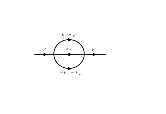
3 IR, BPHZ and DfR: A Two Loop Example

In order to illustrate the correspondence between the BPHZ formalism and IR, we shall compute the $2$-loop correction to the $2$-point function in $\phi^{4}_{4}$ theory in both methods and compare with DfR. The amplitude is depicted in figure $(\ref{setsun})$ (setting-sun diagram). The computation of the finite part of this diagram is notoriously difficult in DR, for instance. However for both IR and DfR [13] it can be readily displayed.

Figure 1: Sunset Diagram

The BPHZ scheme relies on the forest formula to perform the subtraction of the divergences from an amplitude [4]. Let $I_{G}^{\infty}$ be the integrand of such amplitude associated with a graph $G$. Then the subtracted integrand is given by

$$R_{G}=\sum_{U\in\phi}\prod_{\gamma\in U}-t^{d(\gamma)}_{\gamma}I_{G}^{\infty}$$ (35)

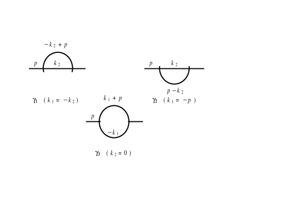
where $\phi$ is the set of all the forests $U$ of $G$, including the empty set , $d(\gamma)$ is the superficial degree of divergence of the subgraph $\gamma$ and $t^{d(\gamma)}$ is the Taylor operator which corresponds to an expansion around $0$ to order $d(\gamma)$ in the external momentum to the subgraph. For the sunset diagram the subgraphs are shown in figure $(\ref{subgraphs})$.

Figure 2: Subgraphs $\gamma_{1},\gamma_{2}$ and $\gamma_{3}$

Therefore we can write $\phi=\{\emptyset,G,\gamma_{1},\gamma_{2},\gamma_{3},G\gamma_{1},G\gamma_{2},G\gamma_{3}\}$. Thus

$$R_{G} = (1-t^{0}_{{\gamma}_{1}}-t^{0}_{{\gamma}_{2}}-t^{0}_{{\gamma}_{3}}-t^{2}_{G}+$$ (36)

$$+ t^{2}_{G}t^{0}_{{\gamma}_{1}}+t^{2}_{G}t^{0}_{{\gamma}_{2}}+t^{G}t^{0}_{{\gamma}_{3}})I_{G}^{\infty}$$

which are ordered so that if $\gamma_{1}\subset\gamma_{2}$ then $t_{\gamma_{1}}$ lies on the right of $t_{\gamma_{2}}$. The amplitude for the sunset diagram is superficially quadratically divergent. It reads

$$\Gamma^{(2)}_{\hbar^{2}}(p) = \frac{g^{2}}{6}\int_{k_{1},k_{2}}I_{G}^{\infty}\,,$$

$$I_{G}^{\infty} = \Delta(k_{1}+p)\Delta(k_{2})\Delta(k_{1}+k_{2})\,\,\,{\mbox{with}}$$

$$\Delta(k) \equiv \frac{1}{k^{2}-\mu^{2}}\,.$$ (37)

Therefore we get, using $(\ref{eq:bphzsub})$,

$$R_{G}=I_{G}^{\infty}-t_{G}^{2}I_{G}^{\infty}-\Delta(k_{2})^{2}(1-t_{G}^{2})\Delta(k_{1}+p)\,.$$ (38)

If one uses a regulator, it can be shown that the term $\Delta(k_{2})^{2}(1-t_{G}^{2})\Delta(k_{1}+p)$ above actually vanishes. This comes from the fact that

$$F(p)=\int_{k}(1-t_{G}^{2})\Delta(k+p)$$

is independent of $p$ and therefore $F(p)=F(0)=0$. Thus according to the BPHZ forest formula, the finite amplitude is obtained through the subtractions:

$$\int_{k_{1},k_{2}}R_{G}=\int_{k_{1},k_{2}}I_{G}^{\infty}-\int_{k_{1},k_{2}}t_{G}^{2}I_{G}^{\infty}\,,$$

$$\int_{k_{1},k_{2}}t_{G}^{2}I_{G}^{\infty}=I_{111}(\mu^{2})-p^{2}I_{112}(\mu^{2})+$$

$$+4\int_{k_{1},k_{2}}(p\cdot k_{1})^{2}\Delta(k_{1})^{3}\Delta(k_{2})\Delta(k_{1}+k_{2})\,\,,$$ (39)

where $I_{mnp}(\mu^{2})$ stands for

$$\int_{k_{1},k_{2}}\frac{1}{(k_{1}^{2}-\mu^{2})^{m}(k_{2}^{2}-\mu^{2})^{n}((k_{1}+k_{2})^{2}-\mu^{2})^{p}}\,.$$ (40)

The integrals $I_{mnp}$ are convergent only if $m+p>2$, $n+p>2$, $m+n>2$, $m+n+p>4$ are satisfied . In order to display the finite part of the setting sun amplitude there is still some work to do in $(\ref{eq:bphzss})$. In particular one would have to adopt a regulator to proceed in this task, the result being regulator independent as guaranteed by the BPHZ scheme. That is to say, the BPHZ scheme guarantees to us is which subtractions one ought to perform in order to render the amplitude finite and that the result is regularization independent.

Now let us evaluate $(\ref{eq:ampss})$ in the light of IR. Because $d(G)=2$ all we need is to apply $(\ref{eq:rr})$ up to $N=2$ in $\Delta(k_{1}+p)$ so to display the infinities in terms of basic divergent integrals which are cleared out of external momenta to get

$$\Delta(k_{1}+p) = \Delta(k_{1})-(p^{2}+2k_{1}\cdot p)\Delta^{2}(k_{1})$$ (41)

$$+ (p^{2}+2p\cdot k_{1})^{2}\Delta^{3}(k_{1})$$

$$- (p^{2}+2p\cdot k_{1})^{3}\Delta^{3}(k_{1})\Delta(k_{1}+p)\,,$$

which enables us to write

$$\frac{6}{g^{2}}\Gamma^{(2)}(p)=I_{111}(\mu^{2})-p^{2}I_{112}(\mu^{2})$$ (42)

$$+ 4\int_{k_{1},k_{2}}(p\cdot k_{1})^{2}\Delta(k_{1})^{3}\Delta(k_{2})\Delta(k_{1}+k_{2})+p^{4}I_{311}$$

$$- \int_{k_{1},k_{2}}(p^{2}+2p\cdot k_{1})^{3}\Delta(k_{1})^{3}\Delta(k_{2})\times$$

$$\times \Delta(k_{1}+k_{2})\Delta(k_{1}+p)\,.$$

Notice that the first three terms in the rhs of the equation above are just the terms which were prescribed to be subtracted using the BPHZ scheme; the fourth term and fifth term (let us call them $F_{4}$ and $F_{5}$ for definiteness ) are clearly divergent but their difference is finite. To see that let us isolate the divergence in both terms as a function of one loop momentum variable only using $(\ref{eq:rr})$. Thus

$$F_{4}=p^{4}I_{log}(\mu^{2})\int_{k_{1}}\Delta(k_{1})^{3}-p^{4}\times$$

$$\times\int_{k_{1},k_{2}}(k_{1}^{2}+2k_{1}\cdot k_{2})\Delta(k_{1})^{3}\Delta(k_{2})^{2}\Delta(k_{1}+k_{2})\,,$$ (43)

whereas

$$F_{5}=I_{log}(\mu^{2})\int_{k_{1}}(p^{2}+2p\cdot k_{1})^{3}\Delta(k_{1})^{3}\Delta(k_{1}+p)$$

$$-\int_{k_{1},k_{2}}(p^{2}+2k_{1}\cdot p)^{3}(k_{1}^{2}+2k_{1}\cdot k_{2})\Delta(k_{1})^{3}\times$$

$$\times\Delta(k_{2})^{2}\Delta(k_{1}+k_{2})\Delta(k_{1}+p)\,\,\,.$$ (44)

By using Feynman parameters to evaluate the first terms in $F_{4}$ and $F_{5}$ one can show that they cancel out. Therefore we can write the finite part ${\cal{F}}=F_{4}-F_{5}$ of the setting-sun amplitude as

$${\cal{F}}=\frac{g^{2}}{6}\int_{k_{1},k_{2}}\Big{(}(p^{2}+2k_{1}\cdot p)^{3}(k_{1}^{2}+2k_{1}\cdot k_{2})\times$$

$$\times\Delta(k_{1})^{3}\Delta(k_{2})^{2}\Delta(k_{1}+k_{2})\Delta(k_{1}+p)-$$

$$-p^{4}(k_{1}^{2}+2k_{1}\cdot k_{2})\Delta(k_{1})^{3}\Delta(k_{2})^{2}\Delta(k_{1}+k_{2})\Big{)}.$$ (45)

In order to make contact with other regularisation/renormalisation frameworks let us take a closer look at the divergent structure of $\Gamma^{(2)}(p)$, namely

$$\frac{g^{2}}{6}\Big{(}I_{111}(\mu^{2})-p^{2}I_{112}(\mu^{2})+$$ (46)

$$+ 4\int_{k_{1},k_{2}}(p\cdot k_{1})^{2}\Delta(k_{1})^{3}\Delta(k_{2})\Delta(k_{1}+k_{2})\Big{)}.$$

It is easy to show that the third term above may be written as

$$p^{2}(I_{112}(\mu^{2})+\mu^{2}I_{113}(\mu^{2}))\,\,\,\,\,\mbox{and that}$$

$$I_{113}=-\frac{b}{2\mu^{2}}I_{log}(\mu^{2})+N\,\,\,\,\ ,\,N\,\,\,\mbox{finite}$$

$$N=-\int_{k_{1},k_{2}}(k_{1}^{2}+2k_{1}\cdot k_{2})$$

$$\times\Delta(k_{1})^{3}\Delta(k_{2})^{2}\Delta(k_{1}+k_{2})\,\,.$$ (47)

Also let us split the logarithmic divergence using $(\ref{eq:scarel})$. Collecting all the results together we have

$$\Gamma^{(2)R}_{\hbar^{2}}(p)=\frac{g^{2}}{6}\Bigg{(}-\frac{b^{2}\,p^{2}}{2}\ln\Big{(}\frac{\lambda^{2}}{\mu^{2}}\Big{)}$$

$$-\int_{k_{1},k_{2}}(p^{4}+\mu^{2}p^{2})(k_{1}^{2}+2k_{1}\cdot k_{2})\Delta(k_{1})^{3}\Delta(k_{2})^{2}\times$$

$$\times\Delta(k_{1}+k_{2})+\int_{k_{1},k_{2}}(p^{2}+2k_{1}\cdot p)^{3}(k_{1}^{2}+2k_{1}\cdot k_{2})\times$$

$$\times\Delta(k_{1})^{3}\Delta(k_{2})^{2}\Delta(k_{1}+k_{2})\Delta(k_{1}+p)\Bigg{)}\,\,,$$ (48)

where

$$\Gamma^{(2)}_{\hbar^{2}}(p)-\Gamma^{(2)R}_{\hbar^{2}}(p)=\frac{g^{2}}{6}(I_{111}(\mu^{2})-\frac{bp^{2}}{2}I_{log}(\lambda^{2}))\,.$$ (49)

The equation $(\ref{eq:pss})$ obtained within IR is the momentum space analogue of the result presented in [13] in DfR,

$$\Gamma_{\hbar^{2}}^{(2)}\Bigg{|}_{R}(x,M)=\frac{g^{2}}{96(4\pi^{2})^{3}}\Big{[}(\square-9\mu^{2})(\square-\mu^{2})$$

$$\Big{(}\mu^{2}K_{0}(\mu x)K_{1}^{2}(\mu x)+\mu^{2}K_{0}^{3}(\mu x)\Big{)}$$

$$+2\pi^{2}\ln\frac{\bar{M}^{2}}{\mu^{2}}(\square-\mu^{2})\delta^{(4)}(x)\Big{]}\,.$$ (50)

Here too, as it was claimed in [13] for DfR, one has been able to display the finite part of the setting sun diagram in a closed and compact form in an easy fashion with the advantage of working directly in the momentum space. Notice that the scale $\lambda$ in (48) is just the analogue of $\bar{M}$ in the equation above and plays the role of scale in the Callan-Symanzik equation satisfied by $\Gamma^{(2)}_{R}(p)$. For instance, for $\mu\rightarrow 0$, $\Gamma^{(2)}_{R}(p^{2})$ is well defined and obbeys

$$\Bigg{(}{{\lambda}}\frac{\partial}{\partial{{\lambda}}}+\beta\frac{\partial}{\partial g}+2\gamma_{\phi}\Bigg{)}\Gamma^{(2)}_{R}(p^{2})=0\,,$$ (51)

from which we may calculate the lowest order value of $\gamma_{\phi}$, namely

$$\gamma_{\phi}=\frac{1}{12}\frac{g^{2}}{(16\pi^{2})^{2}}\,.$$ (52)

In fact it can be shown that $\gamma_{\phi}$ to lowest order is simply the coefficient of the logarithmic divergence $\ln\Lambda^{2}/\mu^{2}$ [27]. By using a general parametrisation for $I_{log}(\lambda^{2})$ [20], viz.

$$I_{log}(\lambda^{2})=b\ln\Big{(}\frac{\Lambda^{2}}{\lambda^{2}}\Big{)}+\eta\,$$ (53)

($\Lambda$ is an UV cutoff and $\eta$ an arbitrary constant) in $(\ref{eq:divss})$ we see that the coefficient of the logarithmic divergence evaluates to $\gamma_{\phi}$ given in $(\ref{eq:gp})$. Alternatively one can apply DR to evaluate $I_{log}(\lambda^{2})$ which gives $b\Gamma(\epsilon)=b(1/\epsilon-\gamma_{E}+O(\epsilon))$.

We can also study the setting sun diagram with arbitrary routing . Let us split the external momentum $p$ between the upper and lower lines in figure $(\ref{setsun})$ so that the amplitude reads

$$\Gamma^{(2)}_{\hbar^{2}}(p,\alpha,\beta) = \frac{g^{2}}{6}\int_{k_{1},k_{2}}\Delta(k_{1}+\alpha p)\Delta(k_{1}+k_{2})\Delta(k_{2}+\beta p)$$ (54)

$$\equiv \frac{g^{2}}{6}\int_{k_{1},k_{2}}I_{G}^{\infty}(\alpha,\beta)\,.$$

with $\alpha+\beta=1$. Using the forest formula one can show within the BPHZ framework that

$$\int_{k_{1},k_{2}}R_{G}=\int_{k_{1},k_{2}}I_{G}^{\infty}(\alpha,\beta)-I_{111}(\mu^{2})+(\alpha+\beta)^{2}I_{112}(\mu^{2})$$

$$-4(\alpha+\beta)^{2}\int_{k_{1},k_{2}}(p\cdot k_{1})^{2}\Delta(k_{1})^{3}\Delta(k_{2})\Delta(k_{1}+k_{2})\,\,.$$ (55)

To work out $(\ref{eq:arbrou})$ within IR, it suffices to expand $\Delta(k_{1}+\alpha p)$ and $\Delta(k_{2}+\beta p)$ using $(\ref{eq:rr})$ up to $N=2$ to get

$$\Gamma^{(2)}_{\hbar^{2}}(p,\alpha,\beta)=I_{111}(\mu^{2})-(\alpha+\beta)^{2}p^{2}I_{112}(\mu^{2})$$

$$+4(\alpha+\beta)^{2}\int_{k_{1},k_{2}}(p\cdot k_{1})^{2}\Delta(k_{1})^{3}\Delta(k_{2})\Delta(k_{1}+k_{2})$$

$$+\,\,\,finite\,\,(\alpha,\beta=1-\alpha).$$ (56)

which turns out to be identical to $(\ref{eq:sperou})$, as it should, because the finite part above can be shown to be independent of $\alpha$. No consistency relations have appeared in this example as the momentum routing independence in the setting sun diagram is trivial. In [21] we calculate the $\beta$ function of $\phi^{4}_{4}$ theory to two loop order within IR.

4 Gluon Self-Energy of QCD

In both abelian and nonabelian gauge field theory the gauge boson self energy is bound by gauge invariance to have the structure $i(p^{2}g_{\mu\nu}-p_{\mu}p_{\nu})\Pi(p^{2})$. For $QCD$, the cancellations that lead to this structure are more complex than for $QED$ and relies on a gauge invariant regularisation framework to handle both the ultraviolet and infrared divergences. It is well known that adding a small mass for the gluon breaks gauge invariance although it may be safely done for the photon.

It will be interesting to see how gauge invariance is implemented in IR for the gluon self energy in connection with the consistency conditions $(\ref{eq:CR4Q1})$ -$(\ref{eq:CR4L2})$. Let $p$ be the external momentum. The diagrams that contribute to the gluon self energy to one loop order are well known: 1) the gluon tadpole $\Pi_{\mu\nu}^{ab}(1)$, 2)the gluon loop $\Pi_{\mu\nu}^{ab}(2)$, 3) the ghost loop $\Pi_{\mu\nu}^{ab}(3)$ and 4) the fermion loop $\Pi_{\mu\nu}^{ab}(4)$. Hence the gluon self energy is given by

$$\Pi^{ab}_{\mu\nu}=\Pi^{ab}_{\mu\nu}(1)+\Pi^{ab}_{\mu\nu}(2)+\Pi^{ab}_{\mu\nu}(3)+\Pi^{ab}_{\mu\nu}(4)$$ (57)

The Feynman rules in momentum space for QCD can be found in any textbook [27]. It is straightforward to show that

$$\Pi^{ab}_{\mu\nu}(1) = -g^{2}C_{2}(G)\delta^{ab}3\int_{k}\frac{g_{\mu\nu}}{k^{2}-\mu^{2}}$$ (58)

$$= -3g^{2}g_{\mu\nu}C_{2}(G)\delta^{ab}I_{quad}(\mu^{2})$$

The gluon loop is equally simple to be displayed within IR. It reads

$$\Pi^{ab}_{\mu\nu}(2)=\frac{1}{2}\int_{k}g^{2}f^{acd}f^{bcd}N_{\mu\nu}\frac{-i}{k^{2}-\mu^{2}}\frac{-i}{(k+p)^{2}-\mu^{2}}\,\,,$$ (59)

where

$$N^{\mu\nu} = [g^{\mu\rho}(p-k)^{\sigma}+g^{\rho\sigma}(2k+p)^{\mu}+g^{\sigma\mu}(-k-2p)^{\rho}]$$ (60)

$$\times [\delta^{\nu}_{\rho}(k-p)_{\sigma}+g_{\rho\sigma}(-2k-p)^{\nu}+\delta^{\nu}_{\sigma}(k+2p)_{\rho}]$$

$$= 2p_{\mu}p_{\nu}-5(p_{\mu}k_{\nu}+p_{\nu}k_{\mu})-10k_{\mu}k_{\nu}$$

$$- g_{\mu\nu}[(p-k)^{2}+(k+2p)^{2}],$$

Using that

$$(p-k)^{2}+(k+2p)^{2}=(k+p)^{2}+k^{2}+4p^{2},$$ (61)

we may write

$$\Pi^{ab}_{\mu\nu}(2) = -\frac{1}{2}g^{2}C_{2}(G)\delta^{ab}[(2p_{\mu}p_{\nu}-4p^{2}g_{\mu\nu})J(p^{2},\mu^{2})$$ (62)

$$- g_{\mu\nu}(2I_{quad}(\mu^{2})+p^{\alpha}p^{\beta}\Upsilon_{\alpha\beta}^{0})$$

$$- 10(\,p_{\nu}J_{\mu}(p^{2},\mu^{2})+J_{\mu\nu}(p^{2},\mu^{2})\,)]\,,$$

whereas the ghost loop is given by

$$\Pi^{ab}_{\mu\nu}(3)=-\int_{k}\frac{i}{k^{2}-\mu^{2}}\frac{i}{[(k+p)^{2}-\mu^{2}]}g^{2}f^{dac}f^{cbd}\times$$

$$\times(p+k)_{\mu}k_{\nu}=-g^{2}\delta^{ab}C_{2}(G)(p_{\nu}J_{\mu}(p^{2},\mu^{2})$$

$$+J_{\mu\nu}(p^{2},\mu^{2}))\,\,,$$ (63)

in which we have used the notation

$$J_{\mu\nu} = \Theta^{(2)}_{\mu\nu}-p^{2}\Theta^{(0)}_{\mu\nu}+4p^{\alpha}p^{\beta}\Theta^{(0)}_{\mu\nu\alpha\beta}$$ (64)

$$+ b\Bigg{[}\frac{p_{\mu}p_{\nu}}{3}\Big{[}\frac{1}{6}-\frac{1}{p^{2}}(p^{2}-\mu^{2})Z_{0}\Big{]}$$ (65)

$$- \frac{p^{2}g_{\mu\nu}}{6}\Big{[}\frac{1}{3}+\frac{1}{2p^{2}}(-p^{2}+4m^{2})Z_{0}\Big{]}\Bigg{]}$$ (66)

$$J_{\mu} = -2p^{\alpha}\Theta_{\alpha\mu}^{(0)}+\frac{1}{2}\,p_{\mu}\,b\,Z_{0}$$ (67)

$$J = I_{log}(\mu^{2})-Z_{0}$$ (68)

with the $Z_{0}$ functions defined as in $(\ref{eq:zks})$

$$Z_{0}=Z_{0}(\mu^{2},\mu^{2},p^{2};\mu^{2})$$ (70)

and

$$\Theta_{\mu\nu}^{(0)} = \int_{k}\frac{k_{\mu}k_{\nu}}{(k^{2}-\mu^{2})^{3}}$$

$$\Theta^{(2)}_{\mu\nu} = \int_{k}\frac{k_{\mu}k_{\nu}}{(k^{2}-\mu^{2})^{2}}$$

$$\Theta_{\mu\nu\alpha\beta}^{(0)} = \int_{k}\frac{k_{\mu}k_{\nu}k_{\alpha}k_{\beta}}{(k^{2}-\mu^{2})^{4}}\,.$$ (71)

Hence we can write $(\ref{eq:CR4L1})$ as $\Upsilon_{\mu\nu}^{0}=g_{\mu\nu}I_{log}(\mu^{2})-4\Theta_{\mu\nu}^{(0)}$, etc. Then it follows that

$$\Pi^{ab}_{\mu\nu}(1)+\Pi^{ab}_{\mu\nu}(2)+\Pi^{ab}_{\mu\nu}(3)=$$

$$=g^{2}C_{2}(G)\delta^{ab}(p^{2}g_{\mu\nu}-p_{\mu}p_{\nu})$$

$$\times\Big{[}-b\frac{2}{9}+\frac{5}{3}\Big{(}I_{log}(\mu^{2})-bZ_{0}\Big{)}\Big{]}.$$ (72)

The fermion loop contribution to the gluon self energy is identical to the vacuum polarization tensor of $QED$ except for the colour and number of fermions ($N_{f}$) factors. It has been computed within IR elsewhere [20]. Here we only write the result in which we have already subtracted $I_{log}(\lambda^{2})$ (that is to say we have employed the minimal subtraction in IR) and set the consistent relations to zero (CIR):

$$\Pi_{\mu\nu}^{ab}(4)=-\frac{i}{144\pi^{2}}g^{2}\frac{N_{f}}{2}\delta^{ab}(p_{\mu}p_{\nu}-p^{2}g_{\mu\nu})\times$$

$$\times\Big{(}12Z_{0}(m_{f}^{2},m_{f}^{2},p^{2};\lambda^{2})+4\Big{)}\,\,.$$ (73)

Now the limit where $\mu\rightarrow 0$ can be safely taken because using $(\ref{eq:scarel})$ and that

$$Z_{0}(\mu^{2},\mu^{2},p^{2};\mu^{2})=\ln\frac{\lambda^{2}}{\mu^{2}}+Z_{0}(\mu^{2},\mu^{2},p^{2};\lambda^{2})\,,$$ (74)

one can show that

$$I_{log}(\mu^{2})-bZ_{0}(\mu^{2},\mu^{2},p^{2};\mu^{2})=I_{log}(\lambda^{2})-$$

$$-bZ_{0}(\mu^{2},\mu^{2},p^{2};\lambda^{2})\,,$$ (75)

and

$$Z_{0}(0,0,p^{2};\lambda^{2})=\ln\frac{p^{2}}{\lambda^{2}}-2\,.$$ (76)

Let us also take the limit of massless fermions. Thus we have,

$$\Pi_{\mu\nu}^{ab}(4)=\frac{i}{144\pi^{2}}g^{2}\frac{N_{f}}{2}\delta^{ab}(p_{\mu}p_{\nu}-p^{2}g_{\mu\nu})[12\mbox{ln}(\bar{\lambda}^{2}/p^{2})-4]\,.$$ (77)

Bringing all the results together enables us to write the complete gluon self energy to one loop order, after minimally subtracting in the sense of IR the divergence expressed by $I_{log}(\lambda^{2})$ and setting $\Upsilon_{\mu\nu}^{0}$ to zero as

$$\Pi_{\mu\nu}^{ab}=\frac{i}{144\pi^{2}}g^{2}\delta^{ab}(p_{\mu}p_{\nu}-p^{2}g_{\mu\nu})\times$$

$$\Big{(}(15C_{2}(R)-6N_{f})\mbox{ln}(\bar{\lambda}^{2}/p^{2})-2C_{2}(R)+2N_{f}\Big{)}$$ (78)

which is just the result obtained in DfR [12] after identifying $\lambda$ with the differential renormalization arbitrary scale ${\bar{M}}$ . Notice that both the massive and massless cases can be straightforwardly handled in IR.

5 Conclusions

In this paper we compared three frameworks namely differential (DfR), implicit (IR) and BPHZ regularisation/renormalisation which being strictly defined in the physical dimension of the underlying theory may overcome the problems which arise when applying dimensional regularisation and variants to dimension specific theories such as supersymmetric, topological or chiral quantum field theories.

The purpose was to motivate the answer to a few questions related to the consistency and applicability of IR in handling infinities in Feynman diagram calculations, namely: 1) study how infrared divergences are treated within this scheme; 2) understand how (nonabelian) gauge invariance can be automatically implemented within a constrained version of IR; 3) define what a minimal subtraction renormalisation is in IR in analogy with dimensional and differential renormalization; 4) argue on the equivalence between IR, DfR and DRed to one loop order and 4) motivate IR as a practical and consistent tool for loop calculations in dimension specific theories.

Since in implicit regularization the divergences are displayed in the form of basic divergent integrals it is natural to ask what is meant by minimal subtraction in such scheme. We have shown that the logarithmic divergences expressed by $I_{log}(\mu^{2})$ can be split as in equation $(\ref{eq:scarel})$ to give rise to am arbitrary scale which plays the role of renormalisation scale in the Callan-Symanzik equation. By subtracting $I_{log}(\lambda^{2})$ when a logarithmic divergence occurs we have a finite part which is identical to the result in differential renormalization (with $\lambda$ playing the role of the arbitrary scale $M$ in DfR) and dimensional regularisation (except for a local counterterm). We define such renormalisation scheme in IR as minimal. In constrained the arbitrary scale is also taken from the logarithmic divergences only [15](functions with singular behaviour worse than logarithmic ($x^{-4}$) are reduced to derivatives of less singular functions without introducing extra dimensionful constants. This is the main ingredient that fixes the renormalization scheme in (constrained) DfR and automatically preserves gauge invariance at least to one loop order. We showed in the calculation of the gluon selfenergy that a constrained version of IR preserves gauge invariance just as it does for abelian gauge theories [19]. Constraining IR amounts to set some well defined finite differences between divergent integrals of the same degree of divergence to zero [19], [20]. Such differences are called consistency relations and were shown to be connected to momentum routing invariance in the loops.

In order to illustrate the relationship between the BPHZ and the IR schemes we have computed the setting sun diagram. The BPHZ scheme is a very powerful tool for all order proofs, for instance, and it delivers unambiguously the terms which ought to be subtracted in order to render the amplitude finite by means of the forest formula. It is a subtraction method which is regularisation independent in what concerns the finite part. In order to proceed the calculation so to extract the finite part, one has to apply ultimately a regularization scheme. However symmetries may be broken in the course of such operations such as gauge invariance. As we have seen within IR certain surface terms are important in order to preserve gauge invariance. Moreover, an expansion around zero in the external momentum potentially breaks the gauge invariant structure of the underlying amplitude. By controlling surface terms and using an identity at the level of the integrand (11) we have verified that IR has control upon gauge invariance at least to one loop order. In other words in IR, the finite part is delivered automatically and no damage is made to the integrand whereas arbitrary local terms are duly parametrised in IR by the consistency relations. A proof of renormalisability to all orders in an alternative fashion to BPHZ has been constructed for $\varphi^{3}_{6}$ theory within IR.

Although we have restricted ourselves to the gluon selfenergy, surely one should verify if the other Slavnov-Taylor identites are satisfied as well, by calculating the vertex functions of $QCD$ [25].

Finally we conclude that both DfR and IR are potentially good frameworks to apply in dimension specific problems in order o avoid ambiguities and spurious anomalies. IR is particularly friendly from the calculational viewpoint with the advantage of working directly in the momentum space. We believe that computations beyond one loop order in Chern-Simons matter theories as well as in supersymmetric models may profit from IR since such method does not modify the underlying theory and operates in the physical dimension of the the theory.

Appendix

The following relations between the functions $Z_{k}$ and $\xi^{mn}$ can be easily checked and simplify the explicit verification of the Ward identity involving the electron self energy and the vertex function.

$$q^{2}\xi_{01}-p.q\xi_{10}={1\over 2}\{Z_{0}(q^{2};m^{2})-Z_{0}(p.q;m^{2})+p^{2}\xi_{00}\}$$ (79)

$$q^{2}\xi_{11}-p.q\xi_{20} = {1\over 2}\Bigg{\{}{-Z_{0}(p+q)^{2};m^{2})\over 2}+{Z_{0}(p^{2};m^{2})\over 2}$$ (80)

$$+ q^{2}\xi_{10}\Bigg{\}}$$

$$q^{2}\xi_{02}-p.q\xi_{11}={1\over 2}\left\{-\left[{1\over 2}+m^{2}\xi_{00}\right]+{p^{2}\over 2}\xi_{10}+{3q^{2}\over 2}\xi_{01}\right\}$$ (81)

$$p^{2}\xi_{20}-p.q\xi_{11}={1\over 2}\left\{-\left[{1\over 2}+m^{2}\xi_{00}\right]+{q^{2}\over 2}\xi_{01}+{3p^{2}\over 2}\xi_{10}\right\}$$ (82)

$$p^{2}\xi_{11}-p.q\xi_{02}={1\over 2}\Big{(}-{1\over 2}Z_{0}((p+q)^{2};m^{2})$$

$$+{1\over 2}Z_{0}(q^{2};m^{2})+p^{2}\xi_{01}\Big{)}\,.$$ (83)

$$\widetilde{Z}(\mu_{\gamma}^{2},m^{2},p,q)=1/2Z_{0}((p-q)^{2},m^{2})-(1/2+\mu_{\gamma}^{2}\xi^{00})$$

$$+1/2(q^{2}+\mu_{\gamma}^{2}-m^{2})\xi^{10}+1/2(p^{2}+\mu_{\gamma}^{2}-m^{2})\xi^{01}\,.$$ (84)

where $\xi^{mn}=\xi^{mn}(m^{2},m^{2},p,q)$ and we have abbreviated

$$Z_{k}(m^{2},m^{2},p^{2};m^{2})\equiv Z_{k}(p^{2};m^{2}).$$ (85)

References

• [1] W. Siegel, Phys. Lett. B84 (1979) 193.
• [2] See for instance: I. Jack and D. T. R. Jones in ”Perspectives in Supersymmetry”, Editor G. Kane, World Scientific, and references therein.
• [3] W. Siegel, Phys. Lett. B94 (1980) 37.
• [4] N. N. Bogolyubov, D. V. Shirkov, Introduction to the theory of the quantised fields, Wiley, 1980; K. Hepp, Comm. Math. Phys.2 (1966) 301; W. Zimmermann, Lectures on Elementary Particles and Quantum Field Theory, Brandeis (1970), edited by S. Deser, M. Grisaru and M. Pendleton; J. H. Lowenstein, BPHZ Renormalisation, Proceedings of NATO Advanced Study Institute, edited by G. Velo and A. S. Wightman, Erice, 1975.
• [5] M. Gomes and B. Schroer, Phys. Rev. D10 (1974) 3525; J. H. Lowenstein, Commun. Math. Phys47 (1976) 53; J. H. Lowenstein and P. K. Mitter, Ann. Phys. 105 (1977) 138; L. C. Albuquerque, M. Gomes and A. J. Silva, Phys. Rev. D62 (2000) 085005.
• [6] G. Dunne, N. Rius, Phys. Lett. B293 (1992) 367.
• [7] D. Z. Freedman, K. Johnson and J. I. Latorre, Nucl. Phys. B371 (1992) 353.
• [8] P. E. Haagensen and J. I. Latorre, Ann. Phys. 221 (1993) 77.
• [9] M. Chaichian and W. F. Chen, Phys. Lett. B409 (1997) 325; W. F. Chen, H. C. Lee and Z. Y. Zhu, Phys. Rev. D55 (1997) 3664; D. Z. Freedman, G. Grignani, K. Johnson and N. Rius, Ann. Phys. 218 (1992) 75.
• [10] F. del Águila, A. Culatti, R. Muñoz Tapia and M. Pérez-Victoria, Nucl. Phys. B537 (1999) 561; Nucl. Phys. B504 (1997) 532 and hep-th/9711474 in Barcelona 1997, Quantum effects in the minimal supersymmetric standard model, 361-373.
• [11] M. Pérez-Victoria, Phys. Lett. B442 (1998) 315.
• [12] F. del Águila and M. Pérez-Victoria, Acta Phys. Polon. B29 (1998)2857.
• [13] P. E. Haagensen and J. I. Latorre, Phys. Lett. B283 (1992) 293.
• [14] P. E. Haagensen and J. I. Latorre, Phys. Lett. B419 (1998) 263.
• [15] F. del Águila and M. Pérez-Victoria, hep-ph/9901291 and Acta Phys. Polon. B28 (1997) 2279.
• [16] T. Hahn and M. Pérez-Victoria, Comput. Phys. Commun. 118 (1999) 153.
• [17] O. A. Battistel, A. L. Mota and M. C. Nemes, Mod. Phys. Lett. A13 (1998) 1597.
• [18] O. A. Battistel, PhD thesis, Federal University of Minas Gerais, Brazil.
• [19] A. P. Baêta Scarpelli, M. Sampaio and M. C. Nemes, Phys. Rev. D63 (2001) 046004.
• [20] A. P. Baêta Scarpelli, M. Sampaio and M. C. Nemes, B. Hiller Phys. Rev. D64 (2001) 046013.
• [21] A. Brizola, O. A. Battistel, M. Sampaio and M. C. Nemes, Mod. Phys. Lett. A14 (1999) 1509.
• [22] S. R. Gobira and M. C. Nemes, Perturbative n-loop renormalization by an implicit regularization technique, hep-th/0102096.
• [23] O. A. Battistel and M. C. Nemes, Phys. Rev. D59 (1999) 055010.
• [24] R. Jackiw in Current Algebra and Anomalies, S. Treiman, R. Jackiw, B. Zumino and E. Witten (Princeton Univ. Press/World Scientific, Singapore, 1985).
• [25] V. O. Rivelles, M. Sampaio, M. C. Nemes, Work in Progress.
• [26] M. T. Grisaru, M. Rocek and W. Siegel, Nucl. Phys. B159 (1979) 429.
• [27] See for instance M. E. Peskin and D. V. Schroeder, An Introduction to Quantum Field Theory, Addison Wesley, 1995.