Complex structure moduli stability in toroidal compactifications

Abstract:

In this paper we present a classification of possible dynamics of closed string moduli within specific toroidal compactifications of Type II string theories due to the NS-NS tadpole terms in the reduced action. They appear as potential terms for the moduli when supersymmetry is broken due to the presence of D-branes. We particularise to specific constructions with two, four and six-dimensional tori, and study the stabilisation of the complex structure moduli at the disk level. We find that, depending on the cycle on the compact space where the brane is wrapped, there are three possible cases: i) there is a solution inside the complex structure moduli space, and the configuration is stable at the critical point, ii) the moduli fields are driven towards the boundary of the moduli space, iii) there is no stable solution at the minimum of the potential and the system decays into a set of branes.

1 Introduction

Branes at angles [1] provide a very rich framework for the construction of compactifications with a chiral spectrum of a very similar structure to the one of the standard model [2, 3, 4, 5, 6, 7]. Generically these models are non-supersymmetric, although some supersymmetric constructions can also be obtained [4]. These configurations are T-dual pictures of branes carrying non trivial bundles wrapping the compact space [8, 9, 2, 10].

There are two types of closed string tadpoles, the Neveu-Schwarz–Neveu-Schwarz (NS-NS) and the Ramond-Ramond (R-R) tadpoles. The cancellation of the R-R tadpoles is a necessary condition for the consistency of the theory. In particular, R-R tadpole cancellation conditions guarantee the absence of chiral anomalies in the low-energy effective theory [1, 2]. However, even if the R-R tapdoles cancel, when supersymmetry is not preserved the NS-NS tadpoles may appear. The system seems to be consistent, but some potentials for the NS-NS fields are generated, signalling that the configuration is not in a stable vacuum, and the string vacuum has to be redefined. This problem has been addressed in several papers [11, 7].

We analyse this problem of the uncancelled NS-NS tadpoles in the context of intersecting branes models, see also Ref. [5]. Given a cycle $\Gamma$ of a homology class on an arbitrary compactification space, we can wrap a brane on it. The system will try to minimise the volume of the brane, inducing a variation of the metric moduli space. When the D-branes wrap a half homology cycle, one can see that the potential depends only on the complex structure moduli. Another way to see it is through the appearance of a NS-NS tadpole term that enters in the effective action as a potential for the complex structure moduli field. One can check that this potential is proportional to the modulus of the periods:

$$|Z_{\Gamma}|=\left|\int_{\Gamma}\Omega\right|\,,$$ (1)

where $\Omega$ is the normalised n-form in a general complex n-dimensional manifold, and $\Gamma$ is a cycle in that class. This form specifies the complex structure of the manifold. Sometimes, depending on the complex structure, this brane is unstable against its decay into other branes.

In this paper we have concentrated on tori of different (even) dimensions, and an arbitrary number of branes. The questions we address here are the following: given a homology class, where is the complex structure moduli going to? Is there a minimum? Is the brane that wraps this cycle stable at the minimum? This problem is analogous to that studied by Moore [12] and Denef [13], in their case related to the construction of stable BPS black holes. We have realised that the minima in both cases are exactly the same. Here we analysed some of the results of Ref. [12] and extrapolated the analysis of the minima to our case. Different phenomena can take place in the flow of these complex structure moduli, like crossing lines of marginal stability that make some branes decay into others [13], etc.

We give here our main conclusions, and leave the description of the details for the following sections. For the 2-dimensional torus the complex structure moduli fields are driven to the boundary of moduli space. In the 4-dimensional torus we find a well differentiated behaviour depending on the wrappings of the branes around the homology cycles. In this case, we analysed a large number of examples, although a general description is absent, as we will discuss below. The most interesting case, however, is the 6-dimensional torus, where we find three different types of behaviours: i) A stable minima can be localised in the interior of the manifold of the complex structure moduli. This will only happen if the cycle is not factorizable . ii) In the case there is only one factorizable cycle, the complex structure moduli are stabilised at some points on the boundary. iii) When the cycle can be decomposed into two factorizable cycles, one can easily see that the minimum is at some point in the interior of the moduli space, but the brane has decayed into a pair of factorizable cycles. However, one can get stable configurations in the interior of the moduli space if one considers more than one factorizable brane. Examples of all the different types of behaviours will be constructed. Note that we have not imposed here the R-R tadpole cancellation conditions, although the dynamics will not be affected if we impose them, as we will discuss later.

When Ramond-Ramond tadpole conditions are imposed, there are, in addition to the vacua where all branes annihilate, some specific vacua where the non-supersymmetric sectors decouple. A trivial example where this happens is that of a pair brane-antibrane at distant points in a compact space. If the distance is larger than the string scale there will be no tachyonic modes. The potential due to the NS-NS tadpoles is proportional to the inverse of the volume of the compact space, and arises from the sum over the winding modes. This means that the potential will be minimised when the volume tends to infinity and the two D-branes are very far from each other. That is what we already know: tadpoles appear in compact spaces, but when the volume goes to infinity its effect is like in a non-compact space. Of course, this is only a tree-level result and quantum corrections are expected. For example, at one-loop, there is an interaction between the pair due to the exchange of massless string excitations. Tree-level and one-loop interactions give two competing effects that can change the direction of the flow.

Moreover, this uncancelled tadpoles could have very interesting physical applications. For instance, the scalar potentials arising from dynamical variations of internal compactification spaces (i.e. complex structures) could be used as inflaton potentials for cosmological inflationary scenarios from strings [14].

In the following sections we will give an introduction to complex structures and moduli spaces, in order to understand the classification of such scalar potentials. We will also give the necessary stability criteria that may help determine phenomenological consequences like inflation. The outline of the paper is the following: in Section 2 we give a general discussion of toroidal compactifications; Sections 3, 4 and 5 discuss some remarkable cases for the two, four and six-dimensional tori, respectively. In the last two Sections we review the work of Moore [12], and give the stability criteria around the various critical points, as well as the general solution for the 6-dimensional torus.

2 Discussion of the models

2.1 Moduli of complex structures

Consider a the 2n-dimensional tori and define a holomorphic n-form $\Omega_{0}$, written as $\Omega_{0}=dz_{1}\wedge...\wedge dz_{n}$, where the complex coordinates $z$ depend on real coordinates $x$ and $y$ as $dz_{i}=dx_{i}+\tau_{ij}dy_{i}$. The $\tau_{ij}$ are complex numbers that specify the complex structure of the manifold. The flat metric on the torus can be written in terms of the complex coordinates as $ds^{2}=dzd\bar{z}$, and the Kähler form is $\omega=dz\wedge d\bar{z}$. The volume of the manifold can be written in terms of the $\Omega_{0}$ form as:

$${\rm Vol}=(-1)^{n(n-1)/2}i^{n}\int\Omega_{0}\wedge\bar{\Omega}_{0}\,.$$ (2)

One can always define a normalised n-form such that its total volume is normalised to 1, i.e. $\Omega\equiv e^{{\cal K}/2}\Omega_{0}$. The volume (2) defines a Kähler potential for the complex structure moduli, ${\cal K}=-\ln({\rm Vol})$, and an induced Kähler metric, $g_{IJ}=\partial_{I}\partial_{J}{\cal K}$, which normalises the complex structure kinetic terms,

$$e^{-2\phi}g_{IJ}\partial_{\mu}Z^{I}\partial^{\mu}Z^{J}\,,$$ (3)

where $I,J$ are coordinates in the complex structure moduli, the $\tau_{ij}$ for instance. These kinetics terms are obtained from the reduction of the Hilbert-Einstein action on the particular manifold. The dependence on the dilaton comes from the closed-string tree-level amplitude.

2.2 Description of the system

We will consider only D6-branes of Type IIA string theory, wrapping 3-cycles on the 6-dimensional compact space, and expanding along the other 4-dimensional Minkowski coordinates. The D6-brane will try to minimise its volume within the same homology class. Depending on the point on the moduli space, the D-brane system can be stable or unstable to the decay to other D-branes whose sum belongs to the same class. The complex structure moduli will vary due to the potential of the NS-NS tadpoles, triggering different effects along their evolution. This can be generalised to T-dual configurations of Type I theory by including orientifold planes and the orientifold images of the branes. We will briefly discuss this case in relation to the R-R tadpole conditions, but we will not analyse it in detail given the huge number of objects involved.

In this section we will review how to obtain these NS-NS tadpoles, the R-R tadpole cancellation conditions, the evolution of complex structure moduli due to the NS-NS tadpoles, the possible decays of D-branes through the lines of marginal stability and a discussion about the stability of the critical points of the potential.

2.3 R-R Tadpoles

In order to obtain a consistent compactification one has to impose the cancellation of all the Ramond-Ramond tadpoles. In particular, they guarantee that the low energy chiral spectrum is anomaly free. These tadpole conditions tell us that the sum of the R-R charges of all branes must be equal to zero in the case of Type IIA compactifications, or equal to the orientifold charge in the case of T-dual compactifications of Type I string theory. These charges are specified by the homology class of the cycles where the branes are wrapped,

$$\sum_{a}\Gamma_{a}=0\,,$$ (4)

for Type IIA theory, and

$$\sum_{a}\Gamma_{a}=q_{o}\Gamma_{o}\,,$$ (5)

for the dual of Type I theory, where $q_{o}$ is the R-R charge of the orientifold plane and $\Gamma_{o}$ is the cycle where it is wrapped. These conditions tell us that, whatever the combinations and decays of branes, the system must have a total R-R charge equal to zero (in the Type IIA case) or equal to $q_{o}\Gamma_{o}$ (in the T-dual of Type I).

In this paper we will analyse configurations where the R-R tadpole conditions are not explicitly satisfied. Only in the last part of the paper we will comment about a way to cancel them by including other branes and antibranes.

The idea is to study the flows of the complex structure fields in these systems for a small set of branes, extracting some general features, and then try to impose these constraints in a more complicated system where the number of branes is substantialy increased and the analysis is not as straightforward. One can always consider adding to one of these simple models some branes, with the charges necessary to cancel the R-R tadpoles, but which are kept as spectators. For example, if we put a brane in a cycle we can always put an antibrane in the same cycle but at large distances from the brane so that they do not develop a tachyonic mode. The R-R tadpoles are immediately cancelled but the NS-NS are added, giving just a factor two in the potential for the complex structure. The difference will appear at one-loop in the open string description (D-brane interaction), but we only consider the disk (tree-level) term. Higher order terms will change the structure of the minima, as we will discuss later. Note that these conditions do not need to be imposed if there are some non-compact coordinates transverse to the branes, as happens in the dyonic black hole constructions of Ref. [15].

2.4 NS-NS Tadpoles

Let us turn now to the more dynamical NS-NS tadpoles. These tadpoles can be written as the volume of the cycle where the D-brane is wrapped, divided by the squared root of the whole volume of the manifold. This can be obtained directly by identification of the tadpole from the cylinder amplitude. In the general case, one obtains these terms by integration of the D-brane action in the compact space. If the NS-NS tadpoles are not cancelled, potential terms will appear in the effective action.

We will consider that each D-brane is volume-minimising and that it preserves some supersymmetry. In our particular case, this means that the brane is wrapping a special Lagrangian manifold. Then the modulus of the period where a BPS D-brane is living gives its volume, and the NS-NS tadpole can be easily written as:

$$V_{a}(\phi,\tau)=e^{-\phi}|Z_{\Gamma_{a}}|=e^{-\phi}\left|\int_{\Gamma_{a}}\Omega\right|\,,$$ (6)

where $\Gamma_{a}$ is the cycle on which the brane wraps. If there is more than one BPS brane the potential becomes

$$V(\phi,\tau)=\sum_{a}V_{a}=e^{-\phi}\sum_{a}\left|\int_{\Gamma_{a}}\Omega\right|\,.$$ (7)

In the T-dual description of Type I theory one should also take into account the contribution from the $2^{9-p}$ orientifold p-planes. Each of these planes has a tension and a R-R charge equal to $-2^{p-4}$ times the tension and the R-R charge of the brane (counting the orientifold images of the brane as independent). For the case of O6-planes, there are 8 of them, with a tension and R-R charge $-4$ times the brane’s. That gives, independently of the dimension of the O-planes, a contribution to the NS-NS tadpoles [5]:

$$V(\phi,\tau)=-32\left|\int_{\Gamma_{o}}\Omega\right|\,.$$ (8)

The NS-NS tadpoles are always positive definite. This is obvious for the Type IIA case, where the tadpoles are the sum of a set of positive real numbers, which means that for this case the absolute minimum of the potential will be the vacuum, a system where all the branes have been annihilated (like in the brane-antibrane case), or when the cycles where the D-branes are wrapped have degenerated to zero volume, in the boundary of moduli space. Indeed, as we will see, depending on the starting point, the system can evolve to the complete absence of branes or towards points where the volume of the branes vanish.

For the T-dual picture of Type I theory one can easily prove that the NS-NS tadpoles,

$$V(\phi,\tau)=\sum_{a}V_{a}=e^{-\phi}\left[\sum_{a}\left|\int_{\Gamma_{a}}\Omega\right|-q_{o}\left|\int_{\Gamma_{o}}\Omega\right|\right]\,,$$ (9)

are always positive definite, by using the triangle inequality and the R-R tadpole conditions (5). This means that an absolute minimum of this configuration will occur when the periods of the branes have the same phases and the same charges as those of the orientifold plane, i.e. all the branes will try to be parallel to the orientifold plane Ref. [5]. The system will be supersymmetric in this case. Of course, another possibility, analogous to the one in the Type II case, is that in which the branes evolve to a system where some cycles can degenerate, or more complicated possibilities if bound states are considered. In this paper we will not analyse configurations with orientifold planes, but is definitely worth studying the extrapolation of our analysis to that case.

2.5 The evolution of the complex structure moduli fields

Here we will discuss the dynamics of the moduli fields. From the point of view of the effective four dimensional theory, the action for the complex structure moduli fields is of the form

$${\cal L}_{4}=e^{-2\phi}g_{IJ}\partial_{\mu}Z^{I}\partial^{\mu}Z^{J}\ -V(\phi,Z^{I})\,.$$ (10)

This effective action has been obtained by dimensional reduction of the 10-dimensional one, where the total volume factors have been absorved in the redefinitions of the fields. From this action, we will see that the complex structure moduli $Z^{I}$ will evolve towards some critical points of the moduli space, which we will characterise below.

Since the variations of the complex structure moduli fields are area-preserving, the Planck constant in the Hilbert-Einstein term does not vary, and therefore the analysis of the stability of the critical points of these potentials $V(\phi,Z^{I})$ can be done in the $Z^{I}$, i.e. the $\tau_{ij}$ coordinates. The stability criteria will not change under the redefinition of $Z^{I}$, needed for obtaining canonically normalised kinetic terms in the Lagrangian (10), only the speed of approach to the critical points. Therefore, in all the figures below, we have drawn the potential $V(\phi,\tau)$ in the $\tau_{ij}$ coordinates. We have also assumed that the dilaton is fixed. Note that, when correctly normalised, the tree-level potential will be proportional to the string coupling constant, $g_{s}=e^{\phi}$. Now, since this potential is always positive, the dilaton will evolve towards weak coupling.

2.6 Lines of marginal stability

Two branes that are intersecting can have tachyonic modes in the spectrum of open string excitations between them. The presence of tachyons is related to the possibility of the decay of the system to another one with the same charges but with a lower volume. Locally these intersecting branes can be seen as two planes. Depending on the dimension of these planes, they can minimise their area [16, 17]. Something similar happens in general Calabi-Yau’s where branes can decay to more stable systems by changing their complex structure [18]. This is a geometrical condition known as the angle criterion [16], that coincides with the computation of the lowest string mode in the NS-NS sector. For every pair of branes intersecting at a point one can define some angles following the procedure given in Refs. [19, 16]. This procedure gives m angles for m-dimensional planes intersecting at a point in a 2m-dimensional space. These angles are called characteristic angles.

We will briefly describe here the six-dimensional toroidal case for factorizable branes. See also Refs. [3, 10]. There are 4 scalar fields that can become tachyonic, with masses,

$$\begin{array}[]{rl}\alpha^{\prime}m^{2}_{1}&={1\over 2\pi}(-\theta_{1}+\theta_{2}+\theta_{3})\,,\\ \alpha^{\prime}m^{2}_{2}&={1\over 2\pi}(\theta_{1}-\theta_{2}+\theta_{3})\,,\\ \alpha^{\prime}m^{2}_{3}&={1\over 2\pi}(\theta_{1}+\theta_{2}-\theta_{3})\,,\\ \alpha^{\prime}m^{2}_{4}&=1-{1\over 2\pi}(\theta_{1}+\theta_{2}+\theta_{3})\,,\end{array}$$ (11)

where the angles $\theta_{i}\in[0,\pi]$. The above masses are related to stability conditions for the pair of branes. If there is no tachyon (notice that only one of the scalar fields can be tachyonic at a time) the two brane system is stable, made of two BPS branes breaking all the supersymmetries. If one of the scalars becomes massless then the system becomes supersymmetric, with the number of supersymmetries related to the number of scalar fields that become massless at the same time. These conditions can be represented in a three dimensional figure in the angle space. The conditions bound a tetrahedron where the different regions are split into:

Figure 1: Angle parameter space for a system of two branes wrapping 3-cycles on $T^{6}$.

Non-supersymmetric and non-tachyonic
(inside the tetrahedron),
${\cal N}=1$ supersymmetric
(faces of the tetrahedron),
${\cal N}=2$ supersymmetric
(edges of the tetrahedron),
${\cal N}=4$ supersymmetric
(vertices of the tetrahedron),
Non-supersymmetric and tachyonic
(outside the tetrahedron).

Lower dimensional cases can be derived from this one by taking one (four-dimensional torus) or two (two-dimensional torus) angles to zero. In the two-dimensional case the system is always tachyonic, signalling the instability of the system to the decay to a lower volume brane. In the four-dimensional case, the system can be supersymmetric or unstable, without the possibility of getting a configuration of two branes that can be volume minimising.

2.7 Critical points

In the 2-dimensional case, the minima of the potential (7) can be studied directly. In the 4-dimensional case, most of the configurations can also be analysed directly. The most interesting case is the 6-dimensional torus. As we have already mentioned, the stable points of the NS-NS potential coincide with the final points of the flow of the attractor equations considered in Refs. [15, 13, 12]. We will follow the analysis of these equations done by Moore in Ref. [12].

In particular, in a 6-dimensional space, Moore shows that if $|Z_{\Gamma}(z)|$ has a stationary point in $z_{*}(\Gamma)\in{\cal M}$ with $|Z_{\Gamma}(z_{*})|\neq 0$ then the 3-form dual to the cycle can be decomposed as $\Gamma=\Gamma^{3,0}+\Gamma^{0,3}$. This stationary point, if it is in the interior of the complex structure moduli space, it must be a local minimum. Then, at the critical point, $\Gamma^{3,0}$ should be proportional to the $\Omega$ form, up to a phase, $\Gamma^{3,0}=-i\bar{C}\Omega$, where $C$ is a complex number. Since $\Gamma\in H^{3}(X,\rm Z\!\!Z)$, then $\Gamma^{0,3}=iC\bar{\Omega}$. The splitting condition above thus translates into

$$2\,\rm Im(\bar{C}\Omega)=\Gamma\,.$$ (12)

Choosing a symplectic basis for $H^{3}(X,\rm Z\!\!Z)$, with internal product $(\alpha_{I},\beta^{J})=\int\alpha_{I}\wedge\beta^{J}=\delta_{I}^{\ J}$, we can write the cycle $\Gamma=p^{I}\alpha_{I}-q_{J}\beta^{J}$, where the coefficients $p_{I},q_{J}$ are integers. The form can be written as $\Omega=X^{I}\alpha_{I}+F_{J}\beta^{J}$, and the splitting condition becomes

$$\bar{C}X^{I}-C\bar{X}^{I} = ip^{I}$$

$$\bar{C}F^{I}-C\bar{F}^{I} = iq^{I}\,,$$ (13)

where $X^{I}$ and $F^{I}$ are the periods along the $\alpha_{I}$ and $\beta^{I}$ cycles, respectively, $X^{I}=\int_{\alpha_{I}}\Omega=\int\Omega\wedge\beta^{I}$. These are $b_{3}$ equations for $b_{3}$ real variables (where $b_{3}$ is the dimension number of $H^{3}(X,\rm I\!R)$), so we can expect the solutions to be isolated points in the complex structure moduli space.

3 The two-dimensional torus

In the case of two-dimensional tori, the special Lagrangian submanifolds are straight lines in the covering space of the torus. There is one for each homology class $\{n[a]+m[b]\}$. The moduli of these curves is ${\cal M}_{\Sigma}=\rm I\!R$ and correspond to translations in the transverse directions to the branes. They can be complexified if Wilson lines are taken into account, see for instance Ref. [13].

In this case, the holomorphic 1-form is $\Omega_{0}=dz$, where $dz=dx+\tau dy$, and $\rm Im\,\tau>0$. The metric on the torus is $ds^{2}=dzd\bar{z}$ and the Kähler form is $\omega=dz\wedge d\bar{z}$. The volume of the torus then becomes

$${\rm Vol}=i\int_{T^{2}}\Omega_{0}\wedge\bar{\Omega}_{0}=\rm Im\,\tau\,.$$ (14)

The Kähler potential for the complex structures is then ${\cal K}=-\ln({\rm Vol})=-\ln(\rm Im\,\tau)$. The Kähler metric in the half plane of complex structures becomes

$$ds^{2}=\frac{d\tau d\bar{\tau}}{(\rm Im\,\tau)^{2}}\,,$$ (15)

and the normalised 1-form:

$$\Omega\equiv e^{{\cal K}/2}\Omega_{0}={dx+\tau dy\over\sqrt{\rm Im\,\tau}}\,.$$ (16)

The periods of the cycles where the D-branes are wrapped become

$$Z_{\Gamma}=\int_{\Gamma}\Omega\,,$$ (17)

which has the interpretation of the volume of the cycle relative to the square root of the volume of the whole torus.

The potential obtained from the NS-NS tadpoles is related to the periods of the brane wrapping the cycle $\Gamma$ by Eq. (6). In this case we have

$$V(\phi,\tau)=e^{-\phi}\frac{|n+\tau m|}{\sqrt{\rm Im\,\tau}}\,.$$ (18)

In the two-dimensional torus we can distinguish two cases:

• if $m=0$, i.e. a brane only wrapping the $[a]$ cycle, the minimum is at $\rm Im\,\tau\rightarrow\infty$, see Fig. 3.

  

  Figure 2: Contour plot for the potential generated by a brane wrapping the $(1,0)$ cycle in a two dimensional torus.

  

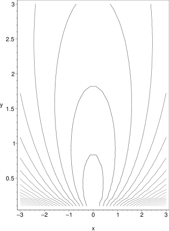
  Figure 3: Contour plot for the potential generated by a brane wrapping the $(0,1)$ cycle in a two dimensional torus.

• if $m\neq 0$ the minimum is at $\tau\rightarrow-n/m$, a real number, see Fig. 3.

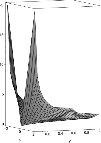
Figure 4: Plot of the potential generated by a brane wrapping the $(1,0)$ cycle in a two dimensional torus.

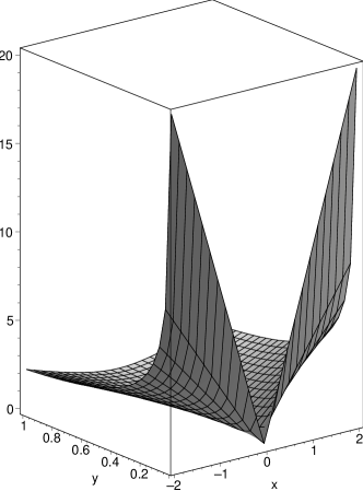
Figure 5: Plot of the potential generated by a brane wrapping the $(1,0)$ cycle in a two dimensional torus.

In both cases the system is driven by this potential to the boundary of the complex structure moduli space, where the volume of the cycle where the brane is wrapped goes to zero. The brane is stable against decays into other type of branes.

The Lagrangian for the complex structure moduli is of the form

$${\cal L}=e^{-2\phi}\frac{\partial_{\mu}\tau\partial^{\mu}\bar{\tau}}{(\rm Im\,\tau)^{2}}-e^{-\phi}\frac{|n+\tau m|}{\sqrt{\rm Im\,\tau}}\,.$$ (19)

By performing a T-duality along the $(1,0)$ direction one can understand this flow as the one responsible for the contraction of the manifold to a point when the D-brane wraps the whole manifold, or its expansion, when T-duality takes the brane to a lower dimensional one, as already mentioned in the introduction.

4 The four-dimensional torus

In this case, the holomorphic 2-form of the 4-dimensional torus is $\Omega_{0}=dz_{1}\wedge dz_{2}$, where $dz_{i}=dx_{i}+\tau_{ij}dy_{i}$ and $\tau_{ij}$ is a 2x2 complex matrix that characterises the complex structure of the torus. The metric on the torus is $ds^{2}=\sum_{i}dz_{i}d\bar{z}_{i}$, and the Kähler form, $\omega=\sum_{i}dz_{i}\wedge d\bar{z}_{i}$. The volume of the torus becomes

$${\rm Vol}=\int_{T^{4}}\Omega_{0}\wedge\bar{\Omega}_{0}={\rm det}\,\tau+{\rm det}\,\bar{\tau}-\tau_{11}\bar{\tau}_{22}-\tau_{22}\bar{\tau}_{11}+\tau_{12}\bar{\tau}_{21}+\tau_{21}\bar{\tau}_{12}\,.$$ (20)

The Kähler potential for the complex structures is as usual, ${\cal K}=-\ln({\rm Vol})$. The Kähler metric in the plane of complex structures, $g_{ij}=\partial_{i}\partial_{j}{\cal K}$. The normalised 2-form becomes $\Omega\equiv e^{{\cal K}/2}\Omega_{0}$. Now we have the 2-cycles dual to the forms $dx^{1}\wedge dx^{2}$, $dx^{i}\wedge dy^{j}$, $dy^{1}\wedge dy^{2}$ that form a basis of $H^{2}(X,\rm I\!R)$. Let us denote the wrapping numbers along these cycles by $q_{0}$, $q_{ij}$, $\tilde{q}_{0}$. The periods of the cycles where the branes are wrapped are given by

$$Z_{\Gamma}=\int_{\Gamma}\Omega={q_{0}+q_{ij}\tau_{ij}+\tilde{q}_{0}\,{\rm det}\,\tau\over\sqrt{\rm Vol}}\,,$$ (21)

which has the interpretation of the volume of the cycle relative to the square root of the volume of the whole manifold. The potential from the NS-NS tadpoles are related to the periods by $V(\phi,\tau)=e^{-\phi}|Z_{\Gamma}|$. Some interesting cases are:

a) If the metric factories into two 2-dimensional tori, i.e. $\tau_{ij}=\delta_{ij}\tau_{i}$, then the volume is

$${\rm Vol}=\prod_{i}\rm Im\,\tau_{i}\,,$$ (22)

and the potential takes a very simple form,

$$V(\phi,\tau)=e^{-\phi}{|q_{0}+\tau_{1}q_{11}+\tau_{2}q_{22}+\tau_{1}\tau_{2}\tilde{q}_{0}|\over\prod_{i}\sqrt{\rm Im\,\tau_{i}}}\,.$$ (23)

Note that in this case we are in a point in the complex structure moduli space where some cycles have zero volume, those with coordinates $q_{12}$ and $q_{21}$. Now let us consider the following subcases:

a.1) If the cycle is also factorizable into two 1-cycles, each one wrapping a two-dimensional torus, then we can denote these 1-cycles by $(r_{1},s_{1})$ and $(r_{2},s_{2})$. The potential is now

$$V(\phi,\tau)=e^{-\phi}\prod_{i}\frac{|r_{i}+s_{i}\tau_{i}|}{\sqrt{\rm Im\,\tau_{i}}}\,.$$ (24)

The problem of analysing this potential reduces to that of the two-dimensional torus. The system is then driven to the boundaries of the complex structure moduli where the 1-cycles collapse.

a.2) We do not consider the cycle factorizable but we keep the same complex structure in both two-dimensional tori, i.e. $\tau_{1}=\tau_{2}=\tau$ . Let us define $q\equiv q_{11}+q_{22}$. Then the potential becomes

$$V(\phi,\tau)=e^{-\phi}\frac{|q_{0}+\tau q+\tau^{2}\tilde{q}_{0}|}{\rm Im\,\tau}\,.$$ (25)

The behaviour of this potential is determined by the sign of the discriminant, $\ \Delta=q^{2}-4q_{0}\tilde{q}_{0}$, of the polynomial:

$$p(\tau)=q_{0}+\tau q+\tau^{2}\tilde{q}_{0}$$ (26)

The different cases are:

a.2.i) If $\Delta>0$, then the two roots are real and are at the boundary. The minimum is in a line joining the two roots. The value of the minimum of the potential is different from zero, $V_{0}(\phi)=e^{-\phi}\Delta/\tilde{q}^{2}_{0}$. See Figs. 7 and 7. Note that the factorizable cycle cases are of this type.

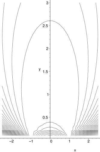
Figure 6: Contour plot of the potential generated by a brane wrapping the $q_{0}=-1$, $q=0$, $\tilde{q}_{0}=1$ cycle in a four dimensional factorizable torus with the same complex structure in the two 2-tori.

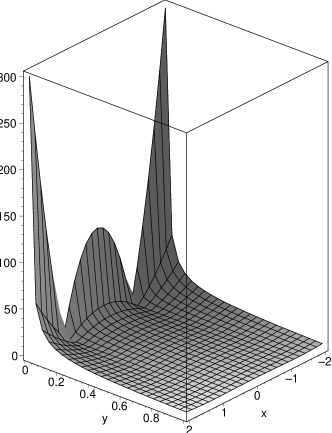
Figure 7: Three dimensional representation of the potential generated by a brane wrapping the $q_{0}=-1$, $q=0$, $\tilde{q}_{0}=1$ cycle in a four dimensional factorizable torus with the same complex structure in the two 2-tori.

a.2.ii) If $\Delta=0$, then the two roots are real and coincide. The minimum is at the root, in the boundary. The value of the minimum of the potential is at zero. See Figs. 9 and 9.

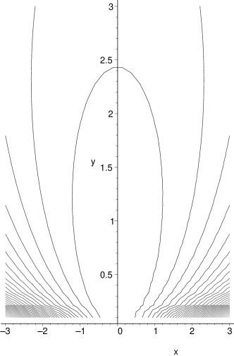
Figure 8: Contour plot of the potential generated by a brane wrapping the $q_{0}=0$, $q=0$, $\tilde{q}_{0}=1$ cycle in a four dimensional factorizable torus with the same complex structure in the two 2-tori.

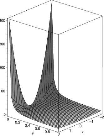
Figure 9: Three dimensional representation of the potential generated by a brane wrapping the $q_{0}=0$, $q=0$, $\tilde{q}_{0}=1$ cycle in a four dimensional factorizable torus with the same complex structure in the two 2-tori.

a.2.iii) If $\Delta<0$, then the two roots are complex conjugates. The minimum is at the root, in the interior of the moduli space of complex structures. The value of the minimum of the potential is at zero. Following the analysis of Moore [12], it seems that there is no BPS state at this point. We will see in some specific examples that this is indeed the case. When $\Delta<0$ the system will cross a line of marginal stability and the brane is expected to decay into another system. Note that this will never be the case when the cycle is factorizable. See Figs. 11 and 11. We will analyse examples of line-crossing in the more interesting case of 6-dimensions.

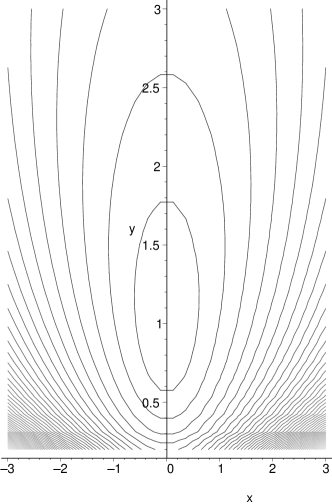
Figure 10: Contour plot of the potential generated by a brane wrapping the $q_{0}=1$, $q=0$, $\tilde{q}_{0}=1$ cycle in a four dimensional factorizable torus with the same complex structure in the two 2-tori.

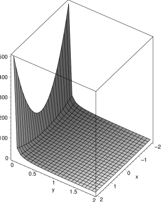
Figure 11: Three dimensional representation of the potential generated by a brane wrapping the $q_{0}=1$, $q=0$, $\tilde{q}_{0}=1$ cycle in a four dimensional factorizable torus with the same complex structure in the two 2-tori.

b) The general case in which the complex structure part of the metric does factorise will not be analysed here. Naive extrapolation from the 6-dimendional analysis ($T^{6}=T^{4}\times T^{2}$) indicates that the system is driven to the boundary ($\Delta=0$). This was expected, since there is a 2-dimensional torus that has always this behaviour.

5 The six-dimensional torus

In this case, the holomorphic 3-form is $\Omega_{0}=dz_{1}\wedge dz_{2}\wedge dz_{3}$, where $dz_{i}=dx_{i}+\tau_{ij}dy_{i}$. The metric on the 6-torus is defined by $ds^{2}=\sum_{i}dz_{i}d\bar{z}_{i}$ and the Kähler form becomes $\omega=\sum_{i}dz_{i}\wedge d\bar{z}_{i}$. The volume of the torus is

$${\rm Vol}=i\int_{T^{6}}\Omega_{0}\wedge\bar{\Omega}_{0}=i\left[{\rm det}\,\tau-{\rm det}\,\bar{\tau}+{\rm tr}(\tau\,{\rm Cof}\,\bar{\tau})-{\rm tr}(\bar{\tau}\,{\rm Cof}\,\tau)\right]\,,$$ (27)

where the cofactor of a matrix is ${\rm Cof}A={\rm det}A\,(A^{-1})^{T}$. The Kähler potential for the complex structures is ${\cal K}=-\ln({\rm Vol})$. The Kähler metric in the plane of complex structures, $g_{ij}=\partial_{i}\partial_{j}{\cal K}$. The normalised 3-form: $\Omega\equiv e^{{\cal K}/2}\Omega_{0}$. Now we have the 3-cycles dual to the following forms, which form a basis of $H^{3}(T^{6},\rm I\!R)$,

$$\begin{array}[]{rl}\alpha_{0}&=dx^{1}\wedge dx^{2}\wedge dx^{3}\,,\\ \alpha_{ij}&={1\over 2}\epsilon_{ilm}\,dx^{l}\wedge dx^{m}\wedge dy^{j}\,,\\ \beta^{ij}&={1\over 2}\epsilon_{jlm}\,dx^{i}\wedge dy^{l}\wedge dy^{m}\,,\\ \beta_{0}&=-dy^{1}\wedge dy^{2}\wedge dy^{3}\,,\end{array}$$

which satisfy the relation:

$$\int_{T^{6}}\alpha_{I}\wedge\beta^{J}=\delta_{I}^{\ J}\,.$$ (28)

The wrapping numbers along these cycles are $q_{0}$, $Q_{ij}$, $P^{ij}$, $p^{0}$, respectively. And the periods of the cycles where the branes are wrapped can be written as

$$Z_{\Gamma}=\int_{\Gamma}\Omega={q_{0}+Q_{ij}\,\tau^{ij}+P^{ij}\,{\rm Cof}\,\tau_{ij}-p^{0}\,{\rm det}\,\tau\over\sqrt{\rm Vol}}\,,$$ (29)

which has the interpretation of the volume of the cycle relative to the square root of the volume of the whole manifold. The potential from the NS-NS tadpoles are related to the periods by $V(\phi,\tau)=e^{-\phi}|Z_{\Gamma}|$. Particular cases are:

a) If the metric factories into three 2-dimensional tori, i.e. $\tau_{ij}=\delta_{ij}\tau_{i}$, then the volume is

$${\rm Vol}=\prod_{i}\rm Im\,\tau_{i}\,,$$ (30)

and the potential takes a very simple form,

$$V(\phi,\tau)=e^{-\phi}{\left|q_{0}+\sum_{i}Q_{ii}\,\tau^{i}+{1\over 2}\sum_{i}P^{ii}\epsilon_{ijk}\tau^{j}\tau^{k}-p^{o}\tau^{1}\tau^{2}\tau^{3}\right|\over\prod_{i}\sqrt{\rm Im\,\tau_{i}}}$$ (31)

Note that in this case we are at a point in the complex structure moduli space where some cycles have zero volume, those with coordinates $Q_{ij}$ and $P^{ij}$, with $i\neq j$. Now let us consider the following subcases:

a.1) If the cycle is also factorizable into two 1-cycles, each one wrapping a two dimensional torus. Let us denote these 1-cycles by $(r_{1},s_{1})(r_{2},s_{2})(r_{3},s_{3})$. The potential is now:

$$V(\phi,\tau)=e^{-\phi}\prod_{i}\frac{|r_{i}+s_{i}\tau_{i}|}{\sqrt{\rm Im\,\tau_{i}}}$$ (32)

The problem of analysing this potential reduces to the two dimensional torus problem. The system is then driven to the boundaries of the complex structure moduli where the 1-cycles collapse.

a.2) We do not consider a factorizable cycle, but we keep the same complex structure in all two-dimensional tori, i.e. $\tau_{i}=\tau$ . Let us define $3q\equiv\sum_{i}Q_{ii}$ and $3p\equiv\sum_{i}P^{ii}$. Then the potential becomes

$$V(\phi,\tau)=e^{-\phi}\frac{|q_{0}+3q\tau+3p\tau^{2}-p^{0}\tau^{3}|}{(\rm Im\,\tau)^{3/2}}$$ (33)

The behaviour of this potential is determined by the sign of the discriminant, $\Delta=12p^{2}q^{2}-(3pq+p^{0}q_{0})^{2}+4(p^{0}q^{3}-q_{0}p^{3})$, of the polynomial:

$$p(\tau)=q_{0}+3q\tau+3p\tau^{2}-p^{0}\tau^{3}\,.$$ (34)

The discriminant gives the number and the type of solutions to $p(\tau)$. As in the four dimensional case, there are 3 subcases:

a.2.i) if $\Delta>0$, there are three real roots, all different. The minimum is in the interior of the complex structure moduli space. The minimum of the potential is not vanishing. Following the interpretation of Moore [12], this means that the corresponding BPS state must exist. See Figs. 13 and 13. Note that this possibility can be achieved with a factorizable cycle. The analysis seems to be in contradiction with the case a.1). But now we are doing a partial analysis by considering all the complex structures equivalent.

However one can get this kind of configurations by taking three factorizables cycles. For example, take $(-1,0)(1,0)(1,0)$, $(0,-1)(0,1)(0,1)$ and $(1,1)(1,1)(1,1)$. We will see this example in detail in the last section.

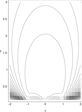
Figure 12: Contour plot of the potential generated by a brane wrapping the $q_{0}=0$, $q=1/3$, $p=0$, $p^{0}=-1$ cycle in a six dimensional factorizable torus with the same complex structure in the three 2-tori.

Figure 13: Three dimensional representation of the potential generated by a brane wrapping the $q_{0}=0$, $q=1/3$, $p=0$, $p^{0}=-1$ cycle in a six dimensional factorizable torus with the same complex structure in the three 2-tori.

a.2.ii) if $\Delta=0$, there are three real roots, but two of them are equal. The minimum is at the boundary. The potential goes to zero at that point in the boundary. See Figs. 15 and 15. Notice that this possibility can be achieved with a factorizable cycle.

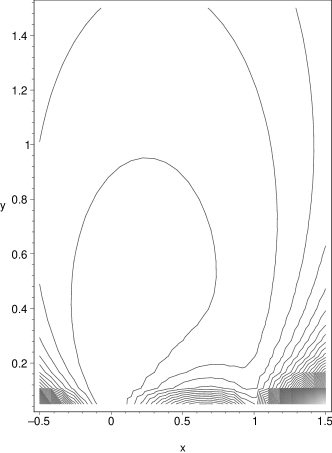
Figure 14: Contour plot of the potential generated by a brane wrapping the $q_{0}=0$, $q=0$, $p=1/3$, $p^{0}=-1$ cycle in a six dimensional factorizable torus with the same complex structure in the three 2-tori.

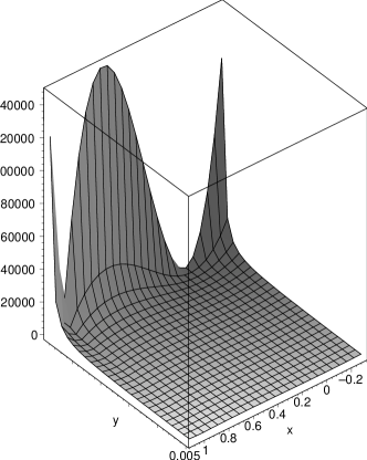
Figure 15: Three dimensional representation of the potential generated by a brane wrapping the $q_{0}=0$, $q=0$, $p=1/3$, $p^{0}=-1$ cycle in a six dimensional factorizable torus with the same complex structure in the three 2-tori.

a.2.iii) if $\Delta<0$, there is one real root and two complex conjugates. The minimum is in the interior of the complex structure moduli. The potential goes to zero at that point. See Figs. 17 and 17. Note that this possibility cannot be achieved with a factorizable cycle. Following Moore we can suspect that the BPS state does not exist. One interesting case when precisely this happens is if we take the combination of two factorizable cycles: $(1,0)(1,0)(1,0)$ and $(0,1)(0,1)(0,1)$. It is easy to check that the minimum is when the two states do not form a bound state. The minimum is at $\tau=i$, where the two branes have angles $\theta_{i}=\pi/2$, i.e. at the centre of the tetrahedron defined by the masses of the scalars that can become tachyons, see Fig. 1. They cannot decay into a bound state.

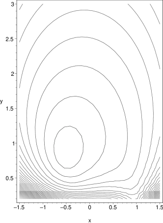
Figure 16: Contour plot of the potential generated by a brane wrapping the $q_{0}=1$, $q=0$, $p=0$, $p^{0}=-1$ cycle in a six dimensional factorizable torus with the same complex structure in the three 2-tori.

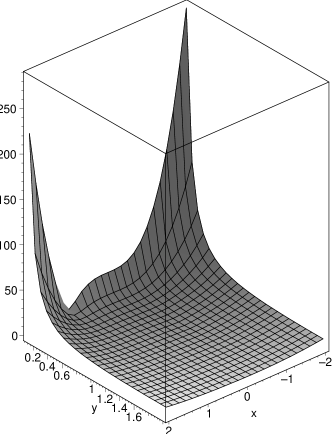
Figure 17: Three dimensional representation of the potential generated by a brane wrapping the $q_{0}=1$, $q=0$, $p=0$, $p^{0}=-1$ cycle in a six dimensional factorizable torus with the same complex structure in the three 2-tori.

b) If the metric is factorisable in two tori, one 4-dimensional, the other 2-dimensional, $T^{6}=T^{4}\times T^{2}$, we recover the previous lower-dimensional cases, and the system will be driven to the boundary. An specific example of this behaviour is to consider that the 3-cycles are factorised into 2-cycles wrapping the 4-dimensional torus and only 1-cycle in the 2-dimensional torus. Then, from the general analysis to be discussed below, one can see that $\Delta=0$.

c) If the metric cannot be factorised. In this case we have to study the general solution, as described in Ref. [12]. As we have seen above, the central charge can be taken to be in this case

$$\int_{\Gamma}\Omega_{0}=q_{0}+Q_{ij}\tau^{ij}+P^{ij}{\rm Cof}\,\tau_{ij}-p^{0}{\rm det}\,\tau\,,$$ (35)

i.e. the period with $\Omega_{0}$. The equations for the critical points (12) become:

$$\begin{array}[]{rl}\rm Im(2\bar{C})&=p^{0}\,,\\ \rm Im(2\bar{C}\,\tau^{ij})&=P^{ij}\,,\\ \rm Im(2\bar{C}\,{\rm Cof}\,\tau_{ij})&=-Q_{ij}\,,\\ \rm Im(2\bar{C}\,{\rm det}\,\tau)&=q^{0}\,.\end{array}$$ (36)

Note that there are $b_{3}=20$ equations and $3\times 3+1=10$ complex unkowns. The solution of this system of equations is described in Ref. [12]. Defining,

$$\begin{array}[]{rl}R&\equiv{\rm Cof}\,P+p^{0}Q\,,\\ M&\equiv 2{\rm det}\,P+(p^{0}q_{0}+{\rm tr}(PQ))p^{0}\,,\\ D&\equiv 2[({\rm tr}PQ)^{2}-{\rm tr}(PQ)^{2}]-(p^{0}q_{0}+{\rm tr}PQ)^{2}+4(p^{0}\,{\rm det}Q-q_{0}\,{\rm det}P)\,,\\ \end{array}$$ (37)

the solution exists for ${\rm det}R\neq 0$, and $D>0$. The result for a general cycle is given by [12]

$$\tau = {1\over 2R}\left[2PQ-(p^{0}q_{0}+{\rm tr}(PQ))+\frac{i}{2}\sqrt{D}\right]\,,$$

$$2\bar{C} = \frac{M}{\sqrt{D}}+ip^{0}\,.$$ (38)

The value of the potential at the critical point is:

$$V_{0}(\phi)=e^{-\phi}\sqrt{D}\,.$$ (39)

There are three different cases:

• $D>0$. There is a relation between $p$, $M$ and ${\rm det}R$, i.e. $4\,{\rm det}R=M^{2}+p^{2}D$. So in this case $D>0\Rightarrow{\rm det}R>0$. There is a solution and the brane exists at the minimum.

• $D=0$. We are in a boundary of the moduli space, $\rm Im\,\tau=0$.

• $D<0$. There is no BPS state with these charges in the minimum. The system will decay into a set of branes.

Let us now compare with the factorizable cycles we are familiar with. Consider generically three 1-cycles $(n_{1},m_{1})(n_{2},m_{2})(n_{3},m_{3})$. Then

$$\begin{array}[]{rl}Q_{ij}&={\rm diag}(n_{2}n_{3}m_{1},n_{1}n_{3}m_{2},n_{2}n_{1}m_{3})\,,\\ P^{ij}&={\rm diag}(m_{2}m_{3}n_{1},m_{1}m_{3}n_{2},m_{2}m_{1}n_{3})\,,\\ q_{0}&=n_{1}n_{2}n_{3}\,,\\ p^{0}&=-m_{1}m_{2}m_{3}\,.\end{array}$$ (40)

It is easy to check that in this case, $D=0$ and ${\rm det}R=0$, so there is no solution inside the complex structure moduli space, but only at the boundaries. This agrees with the previous results that for factorizable cycles the minimum of the potential is at the boundary.

Let us now consider the sum of the $(1,0)(1,0)(1,0)$ and $(0,1)(0,1)(0,1)$ cycles. In this case $q=-p=1$, and $Q=P=0$. Then $D=-1$ is a negative number, which indicates that the bound state will decay into two states. It is easy to prove that for a pair a factorizable branes $D=-I$, where $I$ is the number of intersections between the two branes, a topological number. Then we can say that the bound state of two branes is always unstable and will decay to a two brane system. If the complex structure is factorizable one can easily check that this happens when the angles are $(\pi/2,\pi/2,\pi/2)$, i.e. at the centre of the tetrahedron of Fig. 1. The proof is easy, applying $SL(2,\rm Z\!\!Z)^{3}$ transformations one can take a general two brane factorizable configuration to $a:(1,0)(1,0)(1,0)$ and $b:(n_{1},m_{1})(n_{2},m_{2})(n_{3},m_{3})$. The minimum, as we have said, will be a two-state system. Then the potential is proportional to the sum of the norms of the periods on these cycles. If the complex structure is factorizable, the minimum will be at:

$$m_{i}\,\rm Re\,\tau_{i}+n_{i} = 0$$

$$\prod_{i}|m_{i}|\,\rm Im\,\tau_{i} = 1\,.$$ (41)

The angles $\theta_{i}$ are defined through

$$\tan\,\theta_{i}={m_{i}\,\rm Im\,\tau_{i}\over m_{i}\,\rm Re\,\tau_{i}+n_{i}},$$

such that at the factorizable minimum they all become $\theta_{i}=\pi/2$. The potential at the minimum is precisely $V_{0}=2e^{-\phi}\sqrt{|I|}$.

Note that by adding more factorizable branes we will never recover a general cycle because $Q_{ij}=P_{ij}=0$, for $i\neq j$. That is, factorizable cycles only span diagonal $Q$ and $P$ matrices.

Another very interesting example is the following: Three factorizable cycles:
$(-1,0)(1,0)(1,0)$, $(0,-1)(0,1)(0,1)$ and $(1,1)(1,1)(1,1)$ combine into a general cycle: $q_{0}=p_{0}=0$, $Q=P=1$. Following the same procedure, one can see that $D=3>0$, such that the initial brane configuration decays to the combined system in the minimum. The minimum has a complex structure $\tau=(-{1\over 2}+i{\sqrt{3}\over 4})\,\rm 1\!l$. See Fig. 19, where the potential is plotted keeping the complex structure diagonal and equal for the two dimensional tori. The value of the potential at the minimum is, as expected, $V_{0}(\phi)=e^{-\phi}\sqrt{3}$.

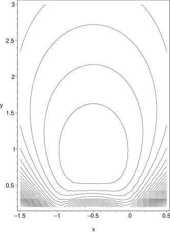
Figure 18: Contour plot of the potential generated by a brane wrapping the $q_{0}=0$, $Q=1$, $P=1$, $p^{0}=0$ cycle in a six dimensional factorizable torus with the same complex structure in the three 2-tori.

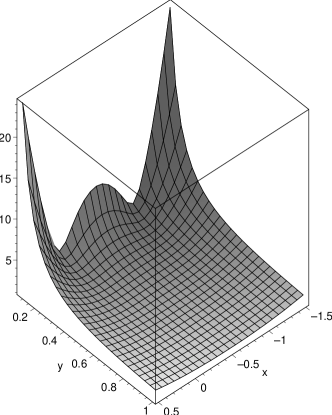
Figure 19: Three dimensional representation of the potential generated by a brane wrapping the $q_{0}=0$, $Q=0$, $P=0$, $p^{0}=-1$ cycle in a six dimensional factorizable torus with the same complex structure in the three 2-tori.

6 Stabilising complex structure moduli. Examples.

In the above examples we have seen different types of behaviours. The evolution of the complex structure fields can drive them to the boundary of the moduli space, to a point in the interior of the moduli space, or can make the brane system to decay by crossing lines of marginal stability. We will described these three very distinct behaviours in this section, with specific examples.

6.1 At the boundary

The simplest example one can construct with this kind of behaviour is a brane wrapping a $(0,1)$ cycle in a two dimensional torus. To cancel the Ramond-Ramond tadpoles one can put an antibrane on the same cycle but far away from the other in such a way that there is no tachyonic mode between them. Of course, the one-loop corrections in the open string description (tree-level in the closed string) will make these two branes approach one another. However, at large distances it is sufficient to analyse only the tree-level potential. Within this aproximation, we find that the effective scalar potential is of the form

$$V(\phi,\tau)=e^{-\phi}{|\tau|\over\sqrt{\rm Im\,\tau}}\,.$$ (42)

The minimum of this potential is at $\tau\rightarrow 0$, i.e. at the boundary. Since there is one brane that is always minimising the volume, the D-brane will never decay to another system, but the brane and antibrane will separate, while the area is kept fixed.

Analogously, a brane wrapping a $(1,0)$ cycle and an antibrane wrapping the same cycle in the opposite side of the torus will cancel the R-R tadpoles and produce a potential of the form

$$V(\phi,\tau)=e^{-\phi}\frac{1}{\sqrt{\rm Im\,\tau}}\,.$$ (43)

Minimisation of this potential drives the brane to $\rm Im\tau\rightarrow\infty$, which means that the two branes will separate and the tachyon will never appear.

This is a very interesting behaviour that contrasts with the one-loop correction responsible for the interaction between the two branes. By adding this interaction, we find two competing effects: NS-NS tadpoles will take branes far apart from eachother, while the D-brane interaction will bring them closer and closer. There is a limiting case in which the two D-branes are just in opposite places in the compact space. The one-loop effect is vanishing (it is a critical but unstable point) and the two branes will separate, never decaying into the vacuum. Alternatively, one can imagine the branes at a distance such that the two effects compensate eachother: the NS-NS tadpole potential, at tree-level, being momentarily cancelled by the one-loop interaction. An interesting physical application of this unstable equilibrium is precisely that which may drive a relatively long period of inflation [14].

6.2 At a point in the interior

The simplest system with this kind of behaviour is a six-dimensional torus with a bound state of two D6-branes, $(1,0)(1,0)(1,0)$ and $(0,1)(0,1)(0,1)$. As we have seen in the previous section, the minimum is at the interior of the complex structure moduli space, where the bound state has decayed to the two-brane system. This system is T-dual to a D9 D3-brane system.

Another system, described above, is the bound state of D6-branes: $(-1,0)(1,0)(1,0)$, $(0,-1)(0,1)(0,1)$ and $(1,1)(1,1)(1,1)$. In this case the bound state is stable in the minimum of the potential. Of course, this system does not satisfy the Ramond-Ramond tadpole conditions. However, we can always put an antibrane wrapped on the same cycle, but far away in the compact space, as we have already discussed above.

7 Conclusions and applications

In this paper we have applied some previous results of Moore [12], derived in the context of BPS quantum black holes, to the analysis of stability of the critical points of the scalar potential due to the NS-NS tadpoles in the context of non-supersymmetric toroidal compactifications, when supersymmetry is broken by the presence of the D-branes. By studying the structure of the potential for some set of branes we have found that the minima can be located at the boundary or at a point in the interior of the complex structure moduli space. Yet another possibility is that, in the evolution to the minimum, the system decay to another one, across lines of marginal stability.

As we have seen in the last section, sometimes the minimum of the potential is not in the vacuum for Type II strings as one would expect, but at a point where the non-supersymmetric spectra decouple. This is analogous to a system of D-branes located at far away points in the compactified space, as in the example mentioned in the introduction. NS-NS tadpoles induce a potential that drives the system to the decompactification limit. That is the usual runaway behaviour for non-supersymmetric compactifications.

It is also interesting to analyse how the flow is corrected by higher loop effects. For instance, the interaction between two branes due to the exchange of closed string modes is a one-loop effect (in the open string description) and can change drastically the behaviour of the system. One can imagine some points where the attraction of a brane-antibrane system (a one loop effect) is compensated by the disk potential (the NS-NS tadpole). This competing effects can have very interesting applications for cosmological scenarios, see for instance Refs. [14].

Some studies for factorizable cycles and metric have been carried out recently for the Type 0’ in Ref. [7], where the system seems to be driven to a point in the interior of the complex structure moduli space and for Type I string theory in Ref. [5]. It would be very interesting to analyse the general structure of the minima, i.e. for non-factorisable cycles and metrics, within the context of non-supersymmetric strings and also for the Type I, where some complex moduli fields are projected out by the orientifold projection.

References

-
[1]
M. Berkooz, M. R. Douglas, R. G. Leigh, “Branes Intersecting at Angles”,
Nucl. Phys. B 480 (1996) 265 [hep-th/9606139].
H. Arfaei, M.M. Sheikh Jabbari, “Different D-brane Interactions”, Phys. Lett. B 394 (1997) 288 [hep-th/9608167].
M.M. Sheikh-Jabbari, “Classification of Different Branes at Angles”, Phys. Lett. B 420 (1998) 279 [hep-th/9710121].
R. Blumenhagen, L. Goerlich, B. Kors, “Supersymmetric Orientifolds in 6D with D-Branes at Angles”, Nucl. Phys. B 569 (2000) 209 [hep-th/9908130]; “Supersymmetric 4D Orientifolds of Type IIA with D6-branes at Angles”, JHEP 0001 (2000) 040 [hep-th/9912204].
S. Forste, G. Honecker, R. Schreyer, “Supersymmetric Orientifolds in 4D with D-Branes at Angles”, Nucl. Phys. B 593 (2001) 127 [hep-th/0008250]. -
[2]
R. Blumenhagen, L. Goerlich, B. Kors, D. Lüst, “Noncommutative
Compactifications of Type I Strings on Tori with Magnetic Background Flux”,
JHEP 0010 (2000) 006 [hep-th/0007024];
“Magnetic Flux in Toroidal Type I Compactification”,
Fortsch. Phys. 49 (2001) 591 [hep-th/0010198].
R. Blumenhagen, B. Kors, D. Lüst, “Type I Strings with F- and B-Flux”, JHEP 0102 (2001) 03 [hep-th/0012156].
G. Aldazabal, S. Franco, L. E. Ibañez, R. Rabadan, A. M. Uranga, “D=4 Chiral String Compactifications from Intersecting Branes”, J. Math. Phys. 42 (2001) 3103 [hep-th/0011073]; “Intersecting Brane Worlds”, JHEP 0102 (2001) 047 [hep-ph/0011132]. - [3] L.E. Ibañez, F. Marchesano, R. Rabadan, “Getting just the Standard Model at Intersecting Branes”, JHEP 0111 (2001) 002 [hep-th/0105155].
- [4] M. Cvetic, G. Shiu, A. M. Uranga, “Chiral Four-Dimensional N=1 Supersymmetric Type IIA Orientifolds from Intersecting D6-Branes”, Nucl. Phys. B 615 (2001) 3 [hep-th/0107166]; “Three-Family Supersymmetric Standard-like Models from Intersecting Brane Worlds”, Phys. Rev. Lett. 87 (2001) 201801 [hep-th/0107143].
- [5] R. Blumenhagen, B. Kors, D. Lüst, T. Ott, “The Standard Model from Stable Intersecting Brane World Orbifolds”, Nucl. Phys. B 616 (2001) 3 [hep-th/0107138].
- [6] D. Cremades, L.E. Ibañez, F. Marchesano, “SUSY Quivers, Intersecting Branes and the Modest Hierarchy Problem”, hep-th/0201205; “Intersecting Brane Models of Particle Physics and the Higgs Mechanism”, hep-th/0203160.
-
[7]
R. Blumenhagen, B. Kors, D. Lüst, “Moduli
Stabilization for Intersecting Brane Worlds in Type 0’ String
Theory”, hep-th/0202024.
- [8] C. Bachas, “A way to break sypersymmetry”, hep-th/9503030.
-
[9]
C. Angelantonj, I. Antoniadis, E. Dudas, A. Sagnotti,
“Type-I strings on magnetised orbifolds and brane transmutation”,
Phys. Lett. B 489 (2000) 223 [hep-th/0007090];
C. Angelantonj, A. Sagnotti, “Type-I vacua and brane transmutation”, Contribution to the Conference on “Quantisation, Gauge Theory, and Strings”, hep-th/0010279. - [10] R. Rabadan, “Branes at angles, torons, stability and supersymmetry”, Nucl. Phys. B 620 (2002) 152 [hep-th/0107036].
-
[11]
W. Fischler and L. Susskind,
“Dilaton Tadpoles, String Condensates And Scale Invariance”,
Phys. Lett. B 171 (1986) 383;
“Dilaton Tadpoles, String Condensates And Scale Invariance. 2”,
Phys. Lett. B 173 (1986) 262.
E. Dudas and J. Mourad, “Brane solutions in strings with broken supersymmetry and dilaton tadpoles”, Phys. Lett. B 486 (2000) 172 [hep-th/0004165].
R. Blumenhagen and A. Font, “Dilaton tadpoles, warped geometries and large extra dimensions for non-supersymmetric strings”, Nucl. Phys. B 599 (2001) 241 [hep-th/0011269]. - [12] G. Moore, “Arithmetic and Attractors”, [hep-th/9807087]; “Attractors and Arithmetic”, [hep-th/9807056].
- [13] F. Denef, “(Dis)assembling Special Lagrangians”, [hep-th/0107152]; “Supergravity flows and D-brane stability”, JHEP 0008 (2000) 050 [hep-th/0005049]; “On the correspondence between D-branes and stationary supergravity solutions of type II Calabi-Yau compactifications”, [hep-th/0010222].
-
[14]
G. Dvali, S.-H. Henry Tye, “Brane Inflation”,
Phys. Lett. B 450 (1999) 72 [hep-ph/9812483].
C.P. Burgess, M. Majumdar, D. Nolte, F. Quevedo, G. Rajesh, R.-J. Zhang, “The Inflationary Brane-Antibrane Universe”, JHEP 0107 (2001) 047 [hep-th/0105204].
G. R. Dvali, Q. Shafi and S. Solganik, “D-brane inflation,” hep-th/0105203.
G. Shiu and S. H. Tye, “Some aspects of brane inflation,” Phys. Lett. B 516 (2001) 421 [hep-th/0106274].
C. Herdeiro, S. Hirano, R. Kallosh, “String Theory and Hybrid Inflation/Acceleration”, JHEP 0112 (2001) 027 [hep-th/0110271].
B. s. Kyae and Q. Shafi, “Branes and inflationary cosmology,” Phys. Lett. B 526 (2002) 379 [hep-ph/0111101].
J. García-Bellido, R. Rabadan, F. Zamora, “Inflationary Scenarios from Branes at Angles”, JHEP 0201 (2002) 036 [hep-th/0112147].
C.P. Burgess, P. Martineau, F. Quevedo, G. Rajesh, R.-J. Zhang, “Brane-Antibrane Inflation in Orbifold and Orientifold Models”, JHEP 0203 (2002) 052 [hep-th/0111025].
R. Blumenhagen, B. Kors, D. Lüst, T. Ott, “Hybrid Inflation in Intersecting Brane Worlds”, hep-th/0202124.
K. Dasgupta, C. Herdeiro, S. Hirano, R. Kallosh, “D3 / D7 Inflationary Model and M Theory”, hep-th/0203019;
N. Jones, H. Stoica, S.-H.Henry Tye, “Brane Interaction as the Origin of Inflation”, hep-th/0203163. -
[15]
S. Ferrara, R. Kallosh, A. Strominger, “N=2 Extremal Black Holes”,
Phys. Rev. D 52 (1995) 5412 [hep-th/9508072].
A. Strominger, “Macroscopic Entropy of Extremal Black Holes”, Phys. Lett. B 383 (1996) 39 [hep-th/9602111].
S. Ferrara, R. Kallosh, “Supersymmetry and Attractors”, Phys. Rev. D 54 (1996) 1514 [hep-th/9602136]; “Universality of Supersymmetric Attractors”, Phys. Rev. D 54 (1996) 1525 [hep-th/9603090]. - [16] D. Nance, “Sufficient conditions for a pair of n-planes to be area minimizing”, Math. Ann. 279 (1987) 161, G. Lawlor, “The angle criterion”, Invent. Math. 95 (1989) 437
- [17] M. R. Douglas, “Topics in D-geometry”, Class. Quant. Grav. 17 (2000) 1057 [hep-th/9910170].
- [18] S. Kachru, J. McGreevy, “Supersymmetric Three-cycles and (Super)symmetry Breaking”, Phys. Rev. D 61 (2000) 026001 [hep-th/9908135].
- [19] R. Harvey, H.B. Lawson, “Calibrated Geometries”, Acta Mathematica 148 (1982) 47.