Determination of quantum symmetries for higher
$ADE$ systems from the modular $T$ matrix

1 Introduction

This article provides a simple tool for the determination, in most cases, of the algebra of quantum symmetries associated with $ADE$ Dynkin diagrams (considered as quantum $su(2)$ objects) or with their generalizations to higher systems (Di Francesco - Zuber diagrams in the case of $su(3)$).

Although a precise general definition of extended Coxeter-Dynkin systems is still lacking, the known examples always contain a “principal” series (the ${\cal A}$ series) and a finite number of “genuine exceptional” cases [24]. The other diagrams of the system are obtained as orbifolds of the genuine diagrams (exceptional or not) and as twists or conjugates (sometimes both) of the genuine diagrams and of their orbifolds. In the case of $su(2)$ (the usual $ADE$ system), we have the principal $A$ series, and the two genuine exceptional cases $E_{6}$ and $E_{8}$; the $D_{2n}$ diagrams are orbifolds of the $A_{4n-3}$ diagrams; the $D_{2n+1}$ diagrams are orbifolds of the $A_{4n-1}$ diagrams and $E_{7}$ is a twist of the $D_{10}$ diagram (itself an orbifold of $A_{17}$). In the case of $su(3)$ (the Di Francesco - Zuber system, slightly amended by A.Ocneanu in [25]), we have the principal series ${\cal A}_{k}$, and three genuine exceptional diagrams: ${\cal E}_{5}$, ${\cal E}_{9}$ and ${\cal E}_{21}$; the others (in particular the other four exceptionals) of the system are obtained from these genuine diagrams by orbifolding, twisting and conjugating.

In some cases, the vector space spanned by the vertices of a given diagram $G$ admits “self-fusion” [27], [28], i.e., it possesses an associative algebra structure with positive integral structure constants (like $A_{n}$, $D_{2n}$, $E_{6}$ and $E_{8}$ for the $su(2)$ system). Sometimes it does not (like $D_{2n+1}$ and $E_{7}$). In all cases, this vector space is a module over the associative algebra of the particular diagram $A$ of the ${\cal A}$ series which has the same Coxeter number (whose definition has to be suitably generalized for the higher systems).

The ${\cal A}$ series is always modular: one can define a representation of $SL(2,\mathbb{Z})$ on the vector space of every diagram of this class (actually this representation factors to a finite group, but we shall not need this information here). The standard generators of this group are called $S$ and $T$. The vector space of the chosen diagram comes with a particular basis, where the basis vectors are associated with graph vertices. The operator $T$ is diagonal on the vertices.

Take $G$ a diagram and $A$ the corresponding member of the ${\cal A}$ series. Being a module over the algebra of $A$, there exist induction-restriction maps between $G$ and $A$ and one can try to define an action of $SL(2,\mathbb{Z})$ on the vector space of $G$, in a way that would be compatible with those maps; this is not necessarily possible. In plain terms: suppose that the vertex $\sigma$ of $G$ appears both in the branching rules (restriction map from $A$ to $G$) of vertices $\tau_{p}$ and $\tau_{q}$ of $A$; one could think of defining the value of the modular generator $T$ on $\sigma$ either as $T(\tau_{p})$ or as $T(\tau_{q})$, but this is ambiguous, unless these two values are equal. In general, there is only a subset $J$ of the vertices of $G$ for which $T$ can be defined: a vertex $\sigma$ will belong to this subset whenever $T$ is constant along the vertices of $A$ whose restriction to $G$ contains $\sigma$.

Following Ocneanu [23], to every diagram $G$ (with or without self-fusion) belonging to a Coxeter-Dynkin system, one can associate a bialgebra $\mathcal{B}G$. This bialgebra should be, technically, a weak Hopf algebra – or quantum groupoid– and we have checked this in a few cases, but we are not aware of any general proof (see our comments in the final section). By using a particular scalar product, one can trade the comultiplication for a multiplication and think that $\mathcal{B}G$ is a di-algebra rather than a bialgebra. There are two –usually distinct – block decompositions for this di-algebra. Blocks of the first type are labelled by points of a diagram $A$ (the member of the ${\cal A}$ series that has same Coxeter number as $G$). Blocks of the second type are labelled by points of another diagram that we call $Oc(G)$. The two sets of orthogonal projectors associated with these two block decompositions can be multiplied with either of these two associative multiplications and this allows one to define associative algebra structures on the vector spaces spanned by the vertices of the two graphs $A$ and $Oc(G)$. We denote these algebras by the same symbol as the graphs themselves. In the particular case where $G$ is a member of the $\mathcal{A}$ series, these algebras coïncide. In all cases, $A$ is an algebra with a single generator and it is commutative. $Oc(G)$, also called “algebra of quantum symmetries of $G$”, is in general an algebra with two generators (only one if $G=A$) and it is not always commutative.

In the cases where $Oc(G)$ is commutative, we observe that this algebra of quantum symmetries can be written in terms of a tensor product of appropriate graph algebras, but the tensor product should be taken above some subalgebra determined by the modular properties of the graph $G$ and we refer to section 3 for a discussion of the several $ADE$ cases. Paradoxically, the simplest cases (besides the $A_{n}$) are those where the diagram $G$ is an exceptional diagram equal to $E_{6}$ or $E_{8}$ (notice that $E_{7}$ does not enjoy self-fusion); in those simple cases $Oc(G)$ is isomorphic with $G\otimes_{J}G$, where $J$ is the particular subalgebra of the graph algebra of $G$ whose determination (using modular considerations) was sketched previously. The tensor product sign, taken “above $J$”, means that we identify $au\otimes b$ and $a\otimes ub$ whenever $u\in J\subset G$. When $Oc(G)$ is not commutative, the method is not fully satisfactory, as we shall see.

The structure of our article is as follows. The first section reminds the reader several useful (but not necessarily widely known) facts about graph algebras and their quantum symmetries. It also precises our notations. The reader already familiar with quantum symmetries of graphs may skip this part. In the second section, we consider the $su(2)$ Coxeter-Dynkin system, i.e., the usual $ADE$ diagrams. For every one of them we simply recover the structure of $Oc(G)$ by our method (which is not fully satisfactory for $D_{2n}$, since the algebra of quantum symmetries of the later is non commutative). We give more details on the $E_{6}$ case because it is both nice and pedagogical. In the third section, we move to the $su(3)$ Coxeter-Dynkin system. After some generalities on these Di Francesco - Zuber graphs and a short description of the cases associated with diagrams of ${\cal A}$ type (which are relatively trivial), we study, in details, also because it is simple enough to be pedagogical, the quantum symmetries of the diagram ${\cal E}_{5}$ (the David star), which is one of the three genuine exceptional cases and is a module over ${\cal A}_{5}$. The technique being now clear, we list only the results for the other two genuine exceptional diagrams ${\cal E}_{9}$ and ${\cal E}_{21}$, i.e., we give their induction-restriction graphs, the values of the modular operator $T$ and, for ${\cal E}_{5}$ and ${\cal E}_{21}$, the structure of their Ocneanu graph. To every point of such a graph, one may associate a “toric matrix” [7], [23], or, equivalently, a twisted partition function in boundary conformal field theory with defect lines [31]; we also give their explicit expressions for the studied $su(3)$ cases, at least those associated with the so-called ambichiral points (to keep the size of this paper reasonable). The list of Di Francesco - Zuber graphs being quite long, we stop at this point, but all the other associated Ocneanu graphs should be obtained by proper generalizations of the study made for $su(2)$; the details can, admittedly, be quite intricate, in particular for those graphs for which $Oc(G)$ is not commutative.

Many topics discussed in the present paper are already known to experts. We believe however that a systematic discussion of the correspondence between the eigenvalues of the $T$ operators and the determination of quantum symmetries is not available elsewhere. Our explicit results concerning the Ocneanu graphs of several exceptional diagrams of the $su(3)$ system seem also to be new, and, we hope, of interest for the reader.

2 About Coxeter-Dynkin graph algebras and their quantum symmetries

2.1 Generalities

To a diagram $G$ belonging to a (possibly higher) Coxeter-Dynkin system, one can associate [23] a bialgebra ${\cal B}(G)$ that we call Ocneanu-Racah-Wigner bialgebra (the precise definition of this bialgebra uses the notion of essential paths on the graph $G$: see our discussion in the Appendix). According to A. Ocneanu (unpublished), this object, also called “algebra of double triangles”, is a semi-simple weak Hopf algebra (or quantum groupoid) — see [3], [21], for general properties of quantum groupoids. We shall not use it explicitly in our paper and it is enough to say that, as a bialgebra, it possesses two associative algebra structures (say “composition $\circ$” and “convolution $\star$”), for which the underlying vector space can be block diagonalized (i.e., decomposed as a sum of matrix algebras) in two different ways. Diagonalization of the convolution product is encoded by a finite dimensional algebra $Oc(G)$ called “algebra of quantum symmetries”. As a vector space, $Oc(G)$ contains one linear generator for every single block of $({\cal B}(G),\star)$. As an algebra, it has a unit called $\underline{0}$ and two generators called ${\underline{1}}_{L}$ and ${\underline{1}}_{R}$, which, when $G$ is a member of an ${\cal A}$ series, coincide. Like the graph algebra of $G$ (when it exists), the algebra $Oc(G)$ comes with a preferred basis. Even when the vector space of $G$ does not admit self-fusion, so that it is only a module over the corresponding ${\cal A}$, the associated object $Oc(G)$ is always both an associative algebra and a bimodule over ${\cal A}\otimes{\cal A}$. This last structure is encoded by a set of matrices that we call “toric matrices”; there is one such matrix for every point of the Ocneanu graph. The multiplicative structure of $Oc(G)$ is fully determined by the two Cayley graphs of multiplication by the generators; the union of these two graphs is called the Ocneanu graph of $G$ and is denoted by the same symbol. In most cases, $Oc(G)$ is isomorphic with a tensor product – over a particular subalgebra $J$ – of two associative and commutative algebras; we write $\stackrel{{\scriptstyle\cdot}}{{\otimes}}\equiv\otimes_{J}$ this tensor product; in these cases, $Oc(G)$ is commutative. When it is not commutative (the case of $D_{2n}$ for the $su(2)$ system), one has also to add some matrix algebra component to this tensor product, in order to take the non-commutativity into account (see [8] for explicit formulas for $D_{2n}$ cases). The two generators of $Oc(G)$ read ${\underline{1}}_{L}=1\stackrel{{\scriptstyle\cdot}}{{\otimes}}0$ and ${\underline{1}}_{R}=0\stackrel{{\scriptstyle\cdot}}{{\otimes}}1$. Their algebraic span are respectively the “left chiral” and “right chiral” parts. The intersection of chiral subalgebras is called “ambichiral” and the vector space spanned by those (preferred) linear generators which belong to none of the chiral parts is called “the supplementary part”. All these structures lead to “nimreps” (non-negative integer valued matrix representations) of certain algebras [30].

From the point of view of Conformal Field Theory, we are interested in partition functions on a torus with defect lines. When there are no defects these partition functions are modular invariant; this is usually not so in the presence of defects. In all cases, they are sesquilinear forms with non negative integer entries defined on the vector space spanned by the characters of an affine Lie algebra $\widehat{\cal G}$. Here we forget this interpretation and replace these characters by vertices of a diagram of type ${\cal A}$. Partition functions are therefore square matrices indexed by these vertices. It was recognized more than seven years ago by A. Ocneanu (published reference is [23]) that “the” modular invariant of Capelli-Itzykson-Zuber [4], [26], [33], for a given $ADE$ diagram $G$, was given by the toric matrix $W_{0}$ associated with the origin $\underline{0}$ of the graph $Oc(G)$. To see an example of how all this works, the reader may look at [7], where toric matrices $W_{x}$ associated with the twelve points $x$ of the graph $Oc(E_{6})$ are calculated. In [29] it was shown (among other things) that to the other points – other than the origin – of a graph $Oc(G)$ can be associated partition functions in boundary conformal field theory (BCFT) with one defect line; these functions are not modular invariant. More general toric matrices (or partition functions) $W_{x,y}$, associated to BCFT with two defect lines, were also introduced in the same paper (note: $W_{x}\equiv W_{x,\underline{0}}$). Fully explicit expressions for the twisted partition functions $W_{x}$ are given in [8], for all $ADE$ cases, by using the formalism introduced in [7]. This was done independently of the work [31]. It should probably be stressed that all these expressions were already obtained (but unpublished) almost eight years ago by A. Ocneanu himself.

The direct determination of the algebra $Oc(G)$, with the definition provided by A. Ocneanu, is not an easy task and the associated graphs are only known (published) for the $su(2)$ Coxeter-Dynkin system. One of the purposes of [7] and [8], besides the calculation of the toric matrices, was actually to give an algebraic construction providing a realization of the algebra $Oc(G)$ in terms of graph algebras associated with appropriated Dynkin diagrams. In the simple cases (paradoxically, for Dynkin diagrams, besides the $A_{n}$ themselves, the “simple” cases happen to be those where $G$ is an exceptional diagram equal to $E_{6}$ or $E_{8}$), the algebra of quantum symmetries is isomorphic with $G\otimes_{J}G$, where $J$ is a particular subalgebra of the algebra of $G$ (we refer to [8] for a discussion of all $ADE$ cases). The tensor product sign, taken “above $J$”, means that we identify $au\otimes b$ and $a\otimes ub$ whenever $u\in J\subset G$. In the last quoted reference, the Ocneanu graphs, determined by Ocneanu himself, had to be taken as an input. This was a weak point in our approach.

For the $su(2)$ Dynkin system, i.e., for $ADE$ diagrams, one purpose of the present article is to show that the structure of $Oc(G)$, can be, in most cases, determined from the eigenvalues of the modular $T$ matrix in the Hurwitz-Verlinde representation [1], [15], [34], associated with the graph algebra of $A_{n}$. The method is general but its implementation depends about the type of diagram considered, i.e., whether it is a member of the ${\cal A}$ series, a genuine exceptional, or if it is obtained as an orbifold or by twisting. In any case, one has first to select a particular subspace $J$ by using the list of eigenvalues of the modular operator $T$ acting on the vertices belonging to the corresponding ${\cal A}$ diagram. In the case of $E_{6}$, for instance, the subset $J$, obtained as explained in the introduction, by using a modular constraint on the induction-restriction rules coming from the $A_{11}$ action, is isomorphic with an $A_{3}$ subalgebra of $E_{6}$ and the Ocneanu algebra $Oc(E_{6})$ is recognized as $E_{6}\stackrel{{\scriptstyle\cdot}}{{\otimes}}_{A_{3}}E_{6}$. Warning: everywhere in this paper, the symbol denoting the diagram also denotes its corresponding associative graph algebra, when it exists; it never refers to the corresponding Lie algebra with the same name (for the higher Coxeter-Dynkin systems, this would not even be an algebra in the usual sense!). The analysis of the $D_{2n}$ cases, where $Oc(G)$ is not commutative, is more subtle.

For the $su(3)$ system, a direct diagonalization of the convolution law $\star$ of the bialgebra ${\cal B}(G)$ was never performed explicitly (or maybe by A. Ocneanu, but this information is not available), and the algebras $Oc(G)$ – or their Cayley graphs – have never been calculated (published) or even properly defined; therefore our method, which can indeed be generalized in a straightforward manner to this more general setting, has a conjectural flavor since we do not compare our results with those that would be obtained by a direct approach. Nevertheless, we have checked, in the case of exceptional graphs of $su(3)$ type, that partition functions (toric matrices) associated with the origin of “our” Ocneanu graphs indeed coincide with the modular invariant partition functions calculated by [13] and that expected sum rules also hold (non trivial equalities between two sums of squares coming from the diagonalization of the two associative structures for a given bialgebra). We obtain also, as a by - product, the list of twisted partition functions corresponding to a given diagram $G$ (there are $24$ of them for the exceptional ${\cal E}_{5}$ case of the $su(3)$ system).

2.2 Useful formulae and notations

For Dynkin diagrams, i.e., the $su(2)$ system, $\kappa$ is the (dual) Coxeter number of the diagram itself. It can be defined, without any reference to the theory of Lie algebras, from the norm $\beta$ of the graph (biggest eigenvalue of the adjacency matrix): $\beta$ is equal to $2\cos\left(\frac{\pi}{\kappa}\right)$. Note that $1<\beta<2$ (see also [14]). For Di Francesco - Zuber graphs, i.e., the $su(3)$ system, the norm $\beta$ is equal to $1+2\cos\left(\frac{2\pi}{\kappa}\right)$. Note that $2<\beta<3$. This again defines the integer $\kappa$. We call it the “generalized Coxeter number of the graph” or “altitude” (like in [11]). We also define $q=exp{\frac{i\pi}{\kappa}}$, so that $q^{2\kappa}=1$. Another integer $h$ characterizes the system of diagrams. For Dynkin diagrams, $h=2$, the (dual) Coxeter number of $su(2)$. For Di Francesco - Zuber graphs, $h=3$, the (dual) Coxeter number of $su(3)$.

The level $k$ of a diagram is defined by the relation $k=\kappa-h$. Notation for graphs: we keep the standard notation for usual Dynkin diagrams, with subscript referring to the number of vertices, i.e., the rank of the corresponding Lie algebra. However, for consistency with the notation used for higher Coxeter-Dynkin systems, it would be better for this subscript to refer to the level $k$ or to the altitude $\kappa$. We may use both notations, but with script capitals in the later case, for instance (Dynkin diagrams): ${\cal A}_{\kappa-2}=A_{\kappa-1}$, ${\cal E}_{10}=E_{6}$, ${\cal E}_{16}=E_{7}$, ${\cal E}_{28}=E_{8}$. In the case of the Di Francesco - Zuber system of graphs, our subscript will always refer to the level. Since $h=3$ for $su(3)$, we have $k=\kappa-3$ for all diagrams of this family. The reader should be warned that this notation is not universally accepted, and some authors may prefer to use the altitude (as an upper index) rather than the level. For instance, the graphs that we call ${\cal E}_{5}$, ${\cal E}_{9}$ and ${\cal E}_{21}$ (like in [25]) were called respectively ${\cal E}^{(8)}$, ${\cal E}^{(12)}_{2}$ and ${\cal E}^{(24)}$ in [11].

In the case of $su(N)$, there are $N-1$ fundamental representations $f$, and therefore $N-1$ graphs $G^{f}$ (see [11]), representing tensor multiplication of irreps by $f$. Since we shall work only with $su(2)$ or $su(3)$, we need only one graph. In the case of $su(2)$, this is clear. In the case of $su(3)$, this graph is associated with one fundamental irrep (say $3$), the other graph associated with its conjugate (say $\overline{3}$) is obtained by reversing all the arrows; adjacency matrices corresponding to the fundamental and to its conjugate are denoted by $G$ and by its transpose $G^{T}$.

For a diagram of type $su(N)$, the graph algebra, when it exists, is faithfully represented (regular representation) by $r\times r$ matrices $G_{a}$. In all cases, $G_{0}$ is the identity matrix and $G_{1}$ is the adjacency matrix. We denote by $r$ the number of vertices of the diagram $G$. The $r$ linear generators $\sigma_{a}$ of $G$, with dual Coxeter number (or altitude) $\kappa$ are then represented by $r$ commuting matrices $G_{a}$.

In the particular case where $G$ is a member of the $A$ system, the generators will be called $\tau_{i}$ and the corresponding matrices will be called $N_{i}$. For a diagram of type $A$ belonging to a given $su(N)$ system, writing down matrices $N_{0}$ (identity) and $N_{1}$ (adjacency matrix) is immediate, and there are always simple recurrence formulae that allow one to compute the matrices $N_{i}$ for all vertices of the $A$ system in terms of $N_{0}$ and $N_{1}$ (thought as the basic representation). These standard recurrence formulae can be obtained for instance by making products of Young frames (see later sections for $su(2)$ and $su(3)$).

The module property (external multiplication) of the vector space associated with a diagram $G$, of level $k$ and possessing $r$ vertices, with respect to an action of the corresponding algebra ${\cal A}_{k}$ is encoded by a set of $s$ matrices $F_{i},{i=0\ldots s-1}$, of dimension $r\times r$, sometimes called “fused graph matrices” (a misleading terminology!): $\tau_{i}\sigma_{a}=\sum_{b}(F_{i})_{ab}\sigma_{b}$. The number $s$ of vertices of ${\cal A}_{k}$ depends on the system: for Dynkin diagrams (${\cal A}_{k}=A_{k+1}$), $s=k+1$; for Di Francesco - Zuber graphs, $s=(k+1)(k+2)/2$. Matrix $F_{0}$ is the identity and matrix $F_{1}=G_{1}$ is also the adjacency matrix of $G$. The other $F$ matrices are determined by imposing that they should obey the same recurrence relation as the $N$ matrices; this ensures compatibility with left multiplication by the algebra ${\cal A}_{k}$. The sets of matrices $F_{i}$, $N_{i}$ and $G_{a}$ of course coincide when $G$ is a diagram of type $A$. The $r$ essential matrices $E_{a}$ are rectangular matrices of dimension $s\times r$ defined by setting $(E_{a})_{ib}=(F_{i})_{ab}$ (the reader should be cautious about the meaning of indices: our indices $i$ or $a$ refer to actual vertices of the graphs but the numbers chosen for labelling rows and columns depend on some arbitrary ordering on these sets of vertices). The particular matrix $E_{0}$ is usually called “intertwiner”, in the statistical physics literature; it also describes “essential paths” emanating from the origin (we shall not need this notion in the present paper). One can check that, for graphs with self-fusion, $E_{a}=E_{0}G_{a}$.

Vertices of the diagram $G$ should be thought of as an analogue of irreducible representations for a subgroup of a group; the irreducible representations of the bigger group are themselves represented by vertices of the graph $A$. In this analogy, the first column of each matrix $F_{i}$ describes the branching rule of $\tau_{i}$ with respect to the chosen subgroup (restriction mechanism). In the same way, the columns of the particular essential matrix $E_{0}$ describe the induction mechanism: the non-zero matrix elements of the column labelled by $\sigma_{b}$ tell us what are those representations $\tau_{i}$ that contain $\sigma_{b}$ in their decomposition (for the branching $A\rightarrow G$).

Let us recall how we compute the (twisted) partition functions $Z_{x,y}$, at least, in the cases where $Oc(G)\simeq G\otimes_{J}G$. Again, we follow the method explained in [7] and refer to [8] for a discussion of all the $ADE$ cases, but another formalism for calculating these quantities was described in [31]. The bimodule structure of $Oc(G)$ with respect to the corresponding ${\cal A}_{k}$ algebra is encoded by matrices $W_{x,y}$ defined as $\tau_{i}.x.\tau_{j}=\sum_{y}(W_{x,y})_{ij}.y$. One sets $W_{x}=W_{x,\underline{0}}$ and obtain the corresponding twisted partition functions as sesquilinear forms $Z_{x,y}=\overline{\chi}W_{x,y}\chi$, or $Z_{x}=Z_{x,\underline{0}}$. Here $\chi$ is a vector in the complex vector space $\mathbb{C}^{s}$. The modular invariant partition function is $Z_{\underline{0}}$ with $\underline{0}=0\stackrel{{\scriptstyle\cdot}}{{\otimes}}0$. The $W_{x,y}$ can be simply obtained from the $W_{x}$ by working out the multiplication table of $Oc(G)$ and decomposing the product $x\times y$ on the basis generators (one of us (R.C.) acknowledges discussions with M. Huerta about this). Practically, once we have the $r$ rectangular matrices $E_{a}$, of dimension $s\times r$ (with $s=\kappa-1$ for $ADE$ diagrams), we first replace by $0$ all the matrix elements of the columns labelled by vertices $b$ that do not belong to the subset $J$ of the graph $G$, call $E_{a}^{red}$ these “reduced” matrices and obtain, for each point $x=a\stackrel{{\scriptstyle\cdot}}{{\otimes}}b$ of the Ocneanu graph $Oc(G)$ (in some cases, $x$ may be a linear combination of such elements), a “toric matrix” $W_{x}=E_{a}\,(E_{b}^{red})^{T}$, of size $s\times s$.

The usual partition function on a torus is calculated by identifying the states at the end of a cylinder through the trace operation. One may incorporate the action of an operator $X$ attached to a non – trivial cycle of the cylinder before identifying the two ends. This operator should commute with the Virasoro generators and its effect is basically to twist the boundary conditions. An explicit expression, in the presence of two twists $X$ and $Y$, was written for such a twisted partition function by [29], [31]; it involves matrix elements of the modular operator $S$. Our own determination of the toric matrices (and corresponding twisted partition functions) uses directly the fusion algebra – i.e., the graph algebra of the $A_{n}$ diagrams. Of course we could, by using the Verlinde formula, express the fusion rule coefficients through the matrix $S$, but in our approach, the diagrams themselves are taken as primary data and we do not need to use this operator at all, at least for the determination of the $W_{x,y}$.

3 $ADE$ diagrams: the $su(2)$ system

3.1 Preliminary remarks

$ADE$ Dynkin diagrams are well known. Their norm (highest eigenvalue of the adjacency matrix) is $2\cos\left(\frac{\pi}{\kappa}\right)=\beta$. Diagrams $A_{\kappa-1}$ have $r$ points $\tau_{j}$, $j=0,\ldots\kappa-2$, with $r=\kappa-1=k+1$ (this defines the level $k$). In the light of McKay correspondance[20], these diagrams appear as quantum analogues of binary polyhedral groups [6], [17], [18]. For $su(2)$, the recurrence formula for adjacency matrices associated with irreps is very well known: we have $N_{0}N_{j}=N_{j}$, $N_{1}N_{j}=N_{j-1}+N_{j+1}$, for $1\leq j\leq\kappa-2$. This is the usual multiplication of spin $j/2$ representation by the fundamental (spin $1/2$). For the diagram $A_{\kappa-1}$, we also have a truncation of the spin rule: $N_{1}N_{\kappa-2}=N_{\kappa-3}$.

Left action of the algebra $A_{\kappa-1}$ on the vector space of a diagram $G$ is defined by setting $F_{0}=G_{0}={\bf 1}_{r\times r}$, $F_{1}=G_{1}$, and compatiblility with left multiplication in $A_{\kappa-1}$ is ensured by imposing the spin rule $F_{1}F_{i}=F_{i-1}+F_{i+1}$, a relation that determines the $F_{i}$’s iteratively.

The modular generator $T$, in the Hurwitz-Verlinde representation, is given by

$$T_{jj^{\prime}}=\exp[2i\pi(\frac{(j+1)^{2}}{4\kappa}-\frac{1}{8})]\delta_{jj^{\prime}}$$

where $j,j^{\prime}$ run from $0$ to $\kappa-2$.

The value of $T$ on the vertex $\tau_{j}$ of $A_{\kappa-1}$ is therefore determined, up to a global phase, by the quantity $\hat{T}=(j+1)^{2}$ mod $4\kappa$, that we will call the “modular exponent” (see also the appendix). The algebras of quantum symmetries $Oc(G)$, for diagrams $G$ of type ADE, are already known, and the corresponding Ocneanu graphs can be found for instance in [5], [7], [8], [23], [30], [31], or also, in the context of the theory of induction of sectors, in [2]. In the present section, the overlap with [8] is important: in the later reference, an algebraic realization of the algebras $Oc(G)$ was given, but the primary data was the Ocneanu graph itself, taken from [23]. In the present section, our aim is neither to describe the algebras of quantum symmetries nor their corresponding graphs, since this is known already, but to show how the modular properties of the diagrams (in particular the table of eigenvalues for the operator $T$) together with the induction-restriction pattern, can be used to recover the known algebras of quantum symmetries. This section also provides a kind of introduction to section 4 where the same techniques will be used to determine the structure of $Oc(G)$ for several diagrams belonging to the $su(3)$ system.

3.2 First example: the $E_{6}$ case

• Graphs.

  The vector space of $E_{6}$ is both an associative (and commutative) algebra with positive integral structure constants (in other words, it admits self-fusion), and it is a module over $A_{11}$. This example is fully studied in [7] (see also [6]); in particular its graph algebra matrices, essential matrices, Ocneanu graph and toric matrices are given there. The $E_{6}$ Dynkin diagram and the corresponding $A$ diagram with same norm (i.e., $A_{11}$) are displayed in Figure 1.

  Figure 1: The $E_{6}$ and $A_{11}$ Dynkin diagrams

  For trees with one branching point (for instance $E_{6}$, $E_{7}$ and $E_{8}$ diagrams), we label (one of) the longest branches with increasing integers starting from $0$, up to the branching point, then we jump to the extremity of the next (clockwise) branch and so on. This is the ordering consistently chosen in [7] and [8].

• Restriction mechanism.

  We look at $E_{6}$ as a module over $A_{11}$. For this, we define an action of $A_{11}$ on $E_{6}$:

  $$\begin{array}[]{ccl}A_{11}\times E_{6}&\rightarrow&E_{6}\\ \tau_{0}.\sigma_{i}&=&\sigma_{i}\\ \tau_{1}.\sigma_{i}&=&\sum^{\prime}\sigma_{j}\end{array}$$

  where $\sum^{\prime}$ runs over the neighbours of $\sigma_{i}$ on the diagram $E_{6}$.
  We have obvious restrictions: $\tau_{0}\hookrightarrow\sigma_{0},\;\tau_{1}\hookrightarrow\sigma_{1}$. To obtain the others, we impose the compatibility condition: $(\tau_{1})^{n}.\sigma_{i}=(\sigma_{1})^{n}.\sigma_{i}$. We therefore calculate the powers of the fundamentals $\tau_{1}$ and $\sigma_{1}$ and compare the results:

  $$\begin{array}[]{lll}(\tau_{1})^{2}=\tau_{0}+\tau_{2},&(\sigma_{1})^{2}=\sigma_{0}+\sigma_{2},&\textrm{so}\qquad\tau_{2}\hookrightarrow\sigma_{2};\\ (\tau_{1})^{3}=2\tau_{1}+\tau_{3},&(\sigma_{1})^{3}=2\sigma_{1}+\sigma_{3}+\sigma_{5},&\textrm{so}\qquad\tau_{3}\hookrightarrow\sigma_{3}+\sigma_{5};\\ \end{array}$$

  and so on.
  In this way, we get the following branching rules $\tau_{i}\hookrightarrow\oplus E_{ij}^{0}\sigma_{j}$ (essential matrix $E_{0}$):

  $$\begin{array}[]{llll}\tau_{0}\hookrightarrow\sigma_{0}&\tau_{1}\hookrightarrow\sigma_{1}&\tau_{2}\hookrightarrow\sigma_{2}&\tau_{3}\hookrightarrow\sigma_{3}+\sigma_{5}\\ \tau_{4}\hookrightarrow\sigma_{2}+\sigma_{4}&\tau_{5}\hookrightarrow\sigma_{1}+\sigma_{5}&\tau_{6}\hookrightarrow\sigma_{0}+\sigma_{2}&\tau_{7}\hookrightarrow\sigma_{1}+\sigma_{3}\\ \tau_{8}\hookrightarrow\sigma_{2}&\tau_{9}\hookrightarrow\sigma_{5}&\tau_{10}\hookrightarrow\sigma_{4}&{}\end{array}$$

  The rectangular $11\times 6$ matrix $E_{0}$ encodes this result, i.e., the above branching rules give us the lines of this matrix. Notice that this determination of $E_{0}$ does not require any calculation involving essential paths (this notion, although extremely nice and useful, is not required at this level).

  Once the adjacency matrix $G_{1}$ is known (read it from the graph), and the essential matrix $E_{0}$ (or intertwiner) determined, we can use the general formulae given in the introduction to determine the $6$ graph matrices $G_{a}$, the $11$ matrices $F_{i}$ and the other essential matrices $E_{a}$ (six of them, including $E_{0}$). Notice that, from the very beginning, we could have proceeded differently, determining first the $F_{i}$ by using both the equation $F_{1}=G_{1}$ and the $su(2)$ rule of composition of spins (recurrence relation); these matrices, in turn, determine the $E_{a}$’s (in particular $E_{0}$).

• Induction mechanism.

  We now look at these previous branching rules, but in the opposite direction: for instance $\sigma_{3}$ comes from $\tau_{3}$ and $\tau_{7}$, so we can write $\sigma_{3}\hookleftarrow(\tau_{3},\tau_{7})$. We get the induction correspondence $E_{6}\hookleftarrow A_{11}$ displayed in Fig 2. This is only another way to write the columns of the $E_{0}$ matrix. We also plot the values of the modular exponent $\hat{T}$ for the vertices $\tau_{i}$’s of $A_{11}$.

  Figure 2: The $E_{6}\hookleftarrow A_{11}$ induction graph and the values of $\hat{T}$ on irreps of $A_{11}$

  From the induction graph we have: $\sigma_{0}\hookleftarrow(\tau_{0},\tau_{6})$, and we notice that the value of the modular matrix $T$ on $\tau_{0}$ and $\tau_{6}$ is the same (also for $\tau_{3}$ and $\tau_{7}$, and for $\tau_{4}$ and $\tau_{10}$). This allows one to assign a fixed value of $T$ to three particular vertices of $E_{6}$: $\hat{T}(\sigma_{0})=1$, $\hat{T}(\sigma_{3})=16$ and $\hat{T}(\sigma_{4})=25$. For every other point of the $E_{6}$ graph, the value of $T$ that would be inherited from the $A_{11}$ graph by this induction mechanism is not uniquely determined (for instance, in the case of $\sigma_{1}$, the values of $\hat{T}$ obtained from $A_{11}$ would be associated with $\tau_{1},\tau_{5}$ and $\tau_{7}$ but these values are not all equal). These elements $\{\sigma_{0},\sigma_{4},\sigma_{3}\}$ span the subalgebra $J=A_{3}$. This subalgebra is known to admit an invariant supplement in the graph algebra of $E_{6}$.

• Quantum symmetries.

  The Ocneanu graph of $E_{6}$ given in [7], [8], [23], [31], is the Cayley graph of multiplication by the two generators of an associative algebra $Oc(E_{6})$ which can be realized (see [7] and [8]) as $E_{6}\otimes_{A_{3}}E_{6}$. It has $12=6\times 6/3$ vertices, three of them being ambichiral, namely $\sigma_{0}\stackrel{{\scriptstyle\cdot}}{{\otimes}}\sigma_{0}$, $\sigma_{0}\stackrel{{\scriptstyle\cdot}}{{\otimes}}\sigma_{3}$ and $\sigma_{0}\stackrel{{\scriptstyle\cdot}}{{\otimes}}\sigma_{4}$. We introduce the symbol $\stackrel{{\scriptstyle\cdot}}{{\otimes}}$ to denote $\otimes_{A_{3}}$ to stress the fact that the tensor product is taken not above the complex numbers but above the subalgebra $J=A_{3}$. This means that $a\,u\stackrel{{\scriptstyle\cdot}}{{\otimes}}b=a\stackrel{{\scriptstyle\cdot}}{{\otimes}}u\,b$ whenever $u\in\{\sigma_{0},\sigma_{4},\sigma_{3}\}$ and $a,b\in E_{6}$. The point that we make, here, is that this subalgebra $A_{3}$ is actually determined as above, by induction, from the eigenvalues of the $T$ operator.

• Dimensions of blocks

  Diagonalization of the two algebra structures of ${\cal B}{E_{6}}$ leads to the quadratic sum rule

  $$dim({\cal B}{E}_{6})=\sum_{i\in A_{11}}d_{i}^{2}=\sum_{x\in Oc(E_{6})}d_{x}^{2}=2512=(2)^{4}(157)^{1}$$

  where $d_{i}=\sum_{a,b\in G}(F_{i})_{ab}$ runs in the list $(6,10,14,18,20,20,20,18,14,10,6)$ and where, for $x=a\stackrel{{\scriptstyle\cdot}}{{\otimes}}b$, $d_{x}=\sum_{i,j\in A_{11}}(G_{a}.G_{b})_{ij}$ runs in the list $(6,8,6,10,14,10,10,14,10,20,28,20)$. This identity follows directly from the fact that ${\cal B}{E_{6}}$ can be written in two different ways as a direct sum of matrix algebras (${\cal B}{E_{6}}$ is semi-simple for both structures).
  We have also the linear sum rule $\sum d_{i}=\sum d_{x}=720=(2)^{4}(3)^{2}(5)^{1}$. Such a linear sum rule also holds “experimentally” in almost all $ADE$ cases (for the $D_{2n}$ cases one has actually to introduce a simple correcting factor, as explained in [31]). In general, there is no reason, for a general bialgebra –even semi-simple for both structures– to give rise to such a linear sum rule. The interpretation of this property is therefore still mysterious. As we shall see in the next part, it also holds for the several examples of diagrams of type $su(3)$ that we have analysed so far.

  There are also quantum sum rules (“mass relations”): define $o(G)\doteq\sum_{a\in G}qdim_{a}^{2}$, where $qdim_{a}$ are the quantum dimensions of the vertices $a$ of $G$ (for example $o(E_{6})=4(3+\sqrt{3})$, $o(A_{11})=24(2+\sqrt{3})$, $o(A_{3})=1+(\sqrt{2}))^{2}=4)$; then, if the diagonalizations of the two algebra structures of ${\cal B}(G)$ are described respectively by ${\cal A}_{k}$, for some $k$, and by $Oc(G)=G\otimes_{J}G$ for some $J$, one can check that $o(Oc(G))$ defined as $\frac{o(G)\times o(G)}{o(J)}$ is equal to $o({\cal A}_{k})$. In the present case, $\frac{o(E_{6})\times o(E_{6})}{o(A_{3})}=o(A_{11})$. This observational fact, properly generalized, holds for all ADE diagrams. Indeed, $o(D_{n})=\frac{1}{2}o(A_{2n-3})$ and $\frac{o(E8)\times o(E8)}{o(J)}=o(A_{29})$, where $o(J)=[1]_{q}^{2}+\left(\frac{[5]_{q}}{[3]_{q}}\right)^{2}$ since the quantum dimensions of vertices $\sigma_{0}$ and $\sigma_{6}$ spanning the subspace $J$ of $E_{8}$ are respectively equal to the q-numbers $[1]_{q}$ and $\frac{[5]_{q}}{[3]_{q}}$ (here $q=\exp(\frac{i\pi}{30})$). In the case of $E_{7}$, we found that $o(Oc(E_{7}))$ defined as $\frac{o(D_{10})\times o(D{10})}{o(J)}$, where $J$ is the subalgebra of $D_{10}$, is equal to $o(A_{17})$. We found also empirically the relation $o(A_{17})=\frac{o(E_{7})\times o(D_{10})}{o(J)}$, where $o(J)=[2]_{q}^{2}+[4]_{q}^{2}+\left(\frac{[4]_{q}}{[3]_{q}}\right)^{2}$ and where the q-numbers $[2]_{q}$, $[4]_{q}$ and $\frac{[4]_{q}}{[3]_{q}}$ are the q-dimensions of the vertices $\sigma_{1}$, $\sigma_{3}$ and $\sigma_{5}$ of $E_{7}$ (here $q=\exp(\frac{i\pi}{18})$). Analoguous quantum sum rules hold for the several examples of diagrams of type $su(3)$ that we have analysed so far. We do not know any general formal proof of these quantum relations.

3.3 The $ADE$ diagrams

We show in this section how all cases relative to the $su(2)$ system can be studied in the same manner.

• $E_{6}$ case.
  It was studied in the last section.

• $E_{8}$ case.
  The cases of $E_{6}$ and $E_{8}$ are very similar. The Dynkin diagram of the $A$ series with same Coxeter number ($\kappa=30$) as $E_{8}$ is $A_{29}$. Like $E_{6}$, the vector space of the diagram $E_{8}$ admits self-fusion (associative algebra structure with positive integral structure constants).

  Figure 3: The $E_{8}\hookleftarrow A_{29}$ induction graph

  The value of $\hat{T}$ on irreps $(\tau_{0},\tau_{1},\tau_{2},\cdots,\tau_{28})$ of $A_{29}$ (equal for $\tau_{j}$ to $(j+1)^{2}$ mod 120) gives:

  $$(\underline{1},4,9,16,25,36,\underline{\underline{49}},64,81,100,\underline{1},22,\underline{\underline{49}},76,105,16,\underline{\underline{49}},84,\underline{1},40,81,4,\underline{\underline{49}},96,25,76,9,64,\underline{1})$$

  We see that $T$ has the same value on vertices $\tau_{j}$ that correspond to $\sigma_{0}$ ($\hat{T}=1$). Same comment for $\sigma_{6}$ ($\hat{T}=49$). We therefore take $J=\{\sigma_{0},\sigma_{6}\}$; this generates a subalgebra which is isomorphic with the algebra of the $A_{2}$ graph. We have indeed $Oc(E_{8})=E_{8}\otimes_{A_{2}}E_{8}$ and the Ocneanu graph has $32=8\times 8/2$ vertices, two of them being ambichiral, namely $\sigma_{0}\stackrel{{\scriptstyle\cdot}}{{\otimes}}\sigma_{0}$ and $\sigma_{0}\stackrel{{\scriptstyle\cdot}}{{\otimes}}\sigma_{6}$. Notice that $\sigma_{6}\stackrel{{\scriptstyle\cdot}}{{\otimes}}\sigma_{6}=\sigma_{0}\stackrel{{\scriptstyle\cdot}}{{\otimes}}\sigma_{0}.$ Dimensions of blocks can be computed as before (see for instance [8]). One writes $dim({\cal B}E_{8})=63136=(2)^{5}(1973)^{1}$ in two different ways as a sum of $29$ or $32$ squares. The linear sum rule gives $\sum d_{i}=\sum d_{x}=1240=(2)^{3}(5)^{1}(31)^{1}$.

• $A_{\kappa-1}$ cases
  The induction-restriction rules from $A_{\kappa-1}$ to itself are of course trivial and the subalgebra $J$ determined by the constancy of $T$ on pre-images is equal to the algebra $A_{\kappa-1}$ itself. The algebra $Oc(A_{\kappa-1})$ equal to $A_{\kappa-1}\otimes_{A_{\kappa-1}}A_{\kappa-1}$ is therefore isomorphic with $A_{\kappa-1}$ itself. The Ocneanu graph coincides with the original Dynkin diagram.

• $D_{2n+1}$ cases
  The Dynkin diagram of the $A$ series with same Coxeter number ($\kappa=4n-2$) as $D_{2n+1}$ is $A_{4n-1}$. Actually (see [19]), $D$ diagrams are $\mathbb{Z}_{2}$ orbifolds of $A$ diagrams.

  Let’s first have a look at the $A_{7}$ case. Its Dynkin diagram and the values of $\hat{T}$ on irreps $\tau_{i}$’s are given in Fig 4.

  Figure 4: The $A_{7}$ diagram and the values of $\hat{T}$

  The algebra of quantum symmetries of $A_{7}$, as we saw, is $A_{7}\otimes_{A_{7}}A_{7}\simeq A_{7}$, but there is also another way to quotient the tensor product if we want $T$ to be well defined in the quotient. We see that the values of $T$ are the same ($\hat{T}=4$) for $\tau_{1}$ and $\tau_{5}$, so we define therefore a map (twist) $\rho:A_{7}\rightarrow A_{7}$ such that:

  $$\rho(\tau_{i})=\tau_{i}\qquad\text{for}\;\,i\in\{0,2,3,4,6\}\qquad\text{and}\quad\rho(\tau_{1})=\tau_{5},\quad\rho(\tau_{5})=\tau_{1}.$$

  Defining then $Oc(D_{5})=A_{7}\otimes_{\rho(A_{7})}A_{7}$ we recover the algebra of quantum symmetry of $D_{5}$.
  This can be generalized for all $D_{2n+1}$ cases. These diagrams do not enjoy self-fusion.
  

• $D_{2n}$ cases
  Starting with the $D_{2n}$ diagram and graph algebra, we obtain the following induction-restriction graph with respect to the corresponding $A$ diagram with the same norm ($A_{4n-3}$).

  Figure 5: The $D_{2n}$-$A_{4n-3}$ induction graph

  The value of $\hat{T}$ on the irreps $\{\tau_{0},\tau_{1},\tau_{2},\cdots,\tau_{2n-1},\tau_{2n},\tau_{2n+1},\cdots,\tau_{4n-6},\tau_{4n-5},\tau_{4n-4}\}$ of $A_{4n-3}$ gives:

  $$T(\tau_{0})=T(\tau_{4n-4})\qquad T(\tau_{2})=T(\tau_{4n-6})\qquad\cdots\qquad T(\tau_{2n-4})=T(\tau_{2n})$$

  These last values are symmetric with respect to the central vertex $\tau_{2n}$.
  We can assign a fixed value of $T$ for the irreps $\{\sigma_{0},\sigma_{2},\cdots,\sigma_{2n-4},\sigma_{2n-2},\sigma_{2n-2}^{{}^{\prime}}\}$ for $D_{2n}$ (marked with a circle in the induction diagram). They span the subalgebra $J$. However, we notice immediately that something special happens here: the two ends of the fork (vertices $\sigma_{2n-2}$ and $\sigma_{2n-2}^{{}^{\prime}}$) are not distinguished by the values of $T$. Actually, the determination of the graph matrices $G_{a}$ for the Dynkin diagram $D_{2n}$ is not as straightforward as for some other cases: looking for an associative algebra determined by this diagram leads to a two-parameter family of solutions, but there is only one solution (up to permutation $G_{2n-2}\leftrightarrow G_{2n-2}^{{}^{\prime}}$) that has correct self fusion, i.e., integrality and positivity of structure constants (a similar phenomenon appears, for example, for the ${\cal E}_{9}$ diagram of the $su(3)$ system). Since $T$ may be defined on any linear combination of these two vertices, it is natural to expect that this arbitrariness is encoded, at the level of the algebra of quantum symmetries, in a “non-commutative geometrical spirit”, by an algebra of $2\times 2$ matrices. $Oc(D_{2n})$ consists indeed of two separate components: the first (usual) is given by $D_{2n}^{trunc}\otimes_{J^{{}^{\prime}}}D_{2n}^{trunc}$, where $D_{2n}^{trunc}$ is the vector space corresponding to the subdiagram spanned by $\{\sigma_{0},\sigma_{1},\sigma_{2},\ldots\sigma_{2n-3}\}$, obtained by removing the fork, and $J^{\prime}=\{\sigma_{0},\sigma_{2},\ldots\sigma_{2n-4}\}$ is the corresponding truncated subset of $J$. The second component is a non-commutative $2\times 2$ matrix algebra reflecting the indistinguishability of $\sigma_{2n-2}$ and $\sigma_{2n-2}^{{}^{\prime}}$. Ambichiral points are associated with the $n+1$ vertices of $J$ (i.e., $n-1$ for the linear branch and $2$ for the fork); we expect therefore that the Ocneanu graph of $D_{2n}$ will have $\frac{(2n-2)(2n-2)}{n-1}+4=4n$ vertices. We could as well say that the number of “effective” points of $J$ is $n$, rather than $n+1$ and notice that $4n=\frac{2n\times 2n}{n}$. This is indeed correct (see [8], [23], [31]). One way to realize the algebra $Oc(D_{2n})$ is to write it as a quotient of the semi-direct product, by $\mathbb{Z}_{2}=\{-,+\}$ of the tensor square of the graph algebra $D_{2n}$. The non-commutativity of the multiplication can be seen, for instance, from the fact that $(2\stackrel{{\scriptstyle\cdot}}{{\otimes}}0,+)(0\stackrel{{\scriptstyle\cdot}}{{\otimes}}0,-)=(2\stackrel{{\scriptstyle\cdot}}{{\otimes}}0,-)$, but $(0\stackrel{{\scriptstyle\cdot}}{{\otimes}}0,-)(2\stackrel{{\scriptstyle\cdot}}{{\otimes}}0,+)=(2^{\prime}\stackrel{{\scriptstyle\cdot}}{{\otimes}}0,-)$. The reader may refer to [8] for another explicit realization of this algebra. In any case, the method followed so far, which is based on the eigenvalues of the $T$ operator, seems to be insufficient to fully determine the Ocneanu graph in that example.

• $E_{7}$ case (related to the $D_{10}$ case)
  For the $D_{10}$ case, something special happens. The corresponding $A$ diagram with the same norm is $A_{17}$, and the value of $T$ in irreps $\{\tau_{0},\tau_{1},\cdots,\tau_{8},\cdots,\tau_{15},\tau_{16}\}$ of $A_{17}$ are:

  $$(1,4,\underline{9},16,25,36,49,64,\underline{9},28,49,0,25,52,\underline{9},40,1)$$

  Figure 6: The $D_{10}$-$A_{17}$ induction graph and the values of $\hat{T}$

  These values are symmetric with respect to the central vertex, as in all $A_{4n-3}$ case. For $A_{17}$, the value of $T$ on the central vertex ($\tau_{8}$) is equal to the value of $T$ on other vertices, namely $\tau_{2}$ and $\tau_{14}$. This gives us another way to define a twist $\rho$ acting on the vertices of $D_{10}$ (this is “the” exceptional twist of the $su(2)$ Coxeter-Dynkin system; existence of this twist is not new, but what we discuss here is its relation with the modular $T$ operator). In other words, we form the tensor product $D_{10}\otimes D_{10}$, but identify $au\otimes b$ with $a\otimes\rho(u)b$ when $u\in\{\sigma_{0},\sigma_{2},\sigma_{4},\sigma_{6},\sigma_{8},\sigma_{8}^{\prime}\}$ and

  $$\begin{array}[]{ccc}\rho(\sigma_{0})=\sigma_{0},&\qquad\qquad\rho(\sigma_{4})=\sigma_{4},&\qquad\qquad\rho(\sigma_{8})=\sigma_{2},\\ \rho(\sigma_{2})=\sigma_{8},&\qquad\qquad\rho(\sigma_{6})=\sigma_{6},&\qquad\qquad\rho(\sigma_{8}^{{}^{\prime}})=\sigma_{8}^{{}^{\prime}}.\end{array}$$

  We obtain the algebra $D_{10}\otimes_{\rho}D_{10}$ which is isomorphic with the algebra of quantum symmetries of the $E_{7}$ diagram. The diagram $E_{7}$ does not enjoy self-fusion.

Remark $1$: The reader will have noticed that we do not necessarily start from a given graph $G$ (for instance $E_{7}$), for which we want to deduce $Oc(G)$. Rather, we first consider all those graphs $G$ which admit a good algebra structure (self fusion), i.e., $A$, $D_{2n}$, $E_{6}$ and $E_{8}$; we then determine, for every one of them, the induced pattern of $T$ eigenvalues by looking at the well determined $A\rightarrow G$ restriction; finally, we build all the possible quotients of $G\otimes G$ over the subalgebras – and possibly twists – determined by the pattern of $T$ values. For example, if we assume that $E_{7}$ is already known to “exist” (as a module over $A_{17}$), and since it does not admit self-fusion, the  only thing that we expect a priori is that its algebra of quantum symmetries $Oc(E_{7})$ will be obtained as a quotient of a tensor product of the algebras $A_{17}$ or $D_{10}$. Therefore, $Oc(E_{7})$ is only the name given to $D_{10}\otimes_{\rho}D_{10}$; the graph $E_{7}$ itself can then be recognized as one of the two subsets of vertices of $Oc(E_{7})$ that linearly generates a module over one of the two chiral parts of the Ocneanu graph (each one being isomorphic with the algebra of $D_{10}$).

Remark $2$: As discussed previously, the method that we follow seems to be insufficient to fully determine $Oc(G)$ when the later is not commutative (cases when a coefficient strictly larger than $1$ appears in the corresponding expression of the modular invariant partition function). These is only one example of this kind for the $su(2)$ system (the $D_{2n}$ diagrams), but there are several such examples for the $su(3)$ system.

4 Di Francesco - Zuber diagrams: the $su(3)$ system

4.1 Preliminary remarks

In the $su(2)$ case, the classification follows an $ADE$ pattern. For $su(n),n\geq 2$ cases, there was no at-hand diagrams to start with, but the list of $su(3)$ diagrams (“generalized Coxeter Dynkin diagrams”) was obtained in 1989 (with CAF $=$ Computer-Aided Flair) by Di Francesco and Zuber in [11]; this list was later shown to be complete by A. Ocneanu, during the Bariloche school at the very beginning of 2000 (actually one of their graphs – the one called ${\cal E}_{3}^{(12)}$ in [11] – had to be removed).

Pictures of the graphs belonging to the Coxeter-Dynkin system of $su(3)$ can be found in [11],[35],[36],[37], and in the book [10]; we refer to [25] and [38] or to the school web page $www.univ-mrs.fr/\sim coque/Bariloche.html$ for the final list. We do not discuss the $su(4)$ system in this paper, but these graphs can also be found in the Ocneanu contribution to the same Bariloche school [25] and on the corresponding web pages.

As recalled earlier, this system contains the principal ${\cal A}$ series and three genuine exceptional cases: ${\cal E}_{5}$, ${\cal E}_{9}$ and ${\cal E}_{21}$. The other diagrams of this system (and in particular the four other exceptional ones) are obtained as twists or as orbifolds of the former list (the “genuine graphs”) , or by using conjugation and twisting on the genuine graphs or on their orbifolds. A member of the ${\cal A}$ series (a Weyl alcove) is obtained by truncation of the diagram (Weyl chamber) of tensorisation of irreps of $su(3)$ by one of the two – conjugate – fundamentals $3$ or $\overline{3}$; for this reason the graphs are oriented (see Fig 7).

Figure 7: The ${\cal A}_{k}$ diagram for $su(3)$ with $(k+1)(k+2)/2$ vertices.

The index refers to the level $k$ of the graph defined by $k=\kappa-h=\kappa-3$. Here $h=3$ is the Coxeter number of the group $SU(3)$ and $\kappa$ is the generalized Coxeter number of the graph (also called “altitude”).

We label the vertices $j$ of the ${\cal A}_{\kappa}$ diagram as $(\lambda_{1},\lambda_{2})$, with $\lambda_{1},\lambda_{2}\geq 0$ and $\lambda_{1}+\lambda_{2}\leq k$. Warning: our labels start from $0$ and not from $1$; many authors follow a different convention. Diagrams ${\cal A}_{k}$ have $r$ points with $r=(k+1)(k+2)/2$.

The action of the modular matrix $T$ on vertices $\tau_{j}\equiv\tau_{(\lambda_{1},\lambda_{2})}$ of ${\cal A}_{k}$ is diagonal and given by:

$$\left(T^{(k)}\right)_{\lambda\mu}=e_{\kappa}\left[-(\lambda_{1}+1)^{2}-(\lambda_{1}+1).(\lambda_{2}+1)-(\lambda_{2}+1)^{2}+\kappa\right]\delta_{\lambda\mu},$$

where $\lambda\doteq(\lambda_{1},\lambda_{2})$, $\mu\doteq(\mu_{1},\mu_{2})$, $e_{\kappa}[x]\doteq\exp\left(\frac{-2i\pi x}{3\kappa}\right)$, and $\kappa=k+3$. We call “modular exponent” the quantity $\hat{T}=-(\lambda_{1}+1)^{2}-(\lambda_{1}+1).(\lambda_{2}+1)-(\lambda_{2}+1)^{2}+\kappa$ mod $3\kappa$.

For $su(3)$, the recurrence formula for adjacency matrices $N_{i}$ associated with irreps is

$$\begin{array}[]{lcll}N_{\lambda,\mu}&=&0&{\text{if}\,\lambda<0\;\,\text{or}\,\mu<0}\\ N_{\lambda,0}&=&N_{1,0}N_{\lambda-1,0}-N_{\lambda-2,1}&{}\\ N_{\lambda,\mu}&=&N_{1,0}N_{\lambda-1,\mu}-N_{\lambda-1,\mu-1}-N_{\lambda-2,\mu+1}&{\text{if}\,\mu\neq 0}\\ N_{0,\lambda}&=&N_{\lambda,0}^{T}&{}\end{array}$$

Remember that fused adjacency matrices $F_{i}$, associated with any graph $G$ of the same level, are determined by the same recurrence relations (but the seed is different: $F_{1}=G_{1}$, the adjacency matrix of $G$).

In some cases the vector space generated by the vertices of a Di Francesco - Zuber graph is an algebra with positive integral structure constants (self fusion). In all cases it is a module over the algebra of type ${\cal A}$ with the same Coxeter number. For an ${\cal A}$ graph, the identity element is $(0,0)$; vertices $(1,0)$ and $(0,1)$, corresponding classically to the two representations of dimension $3$, are the two complex conjugated generators. As always, a given diagram encodes the multiplication by the generators in the following sense: multiplication of an irrep $(\lambda_{1},\lambda_{2})$ by the left generator $(1,0)$ is given by the sum of the irreps which are connected to $(\lambda_{1},\lambda_{2})$ by an incoming arrow, whereas multiplication by the right generator $(0,1)$ is given by the sum of the irreps which are connected to $(\lambda_{1},\lambda_{2})$ by an outgoing arrow. To label vertices, some readers may prefer Young frames (diagrams) rather than a notation using weights. The correspondance is as follows: $(\lambda_{1},\lambda_{2})$ correspond to Young diagrams $Y(p=\lambda_{1}+\lambda_{2},q=\lambda_{2})$ with two rows, $p$ boxes on the first row, and $q$ boxes on the second row. Graphs whose vector space possesses self fusion have a unit, and one of the two generators is located at the extremity of the (single) oriented edge that leaves the origin (reverse the arrows to get the other generator). Triality i.e.,   $\{0,1,2\in\mathbb{Z}/3\mathbb{Z}\}$ is well defined and compatible with internal multiplication (if it exists) or with external multiplication by vertices of the corresponding ${\cal A}$ graph; it is represented by different choices of “colors” of vertices on the pictures. There is also a conjugacy transformation $\sigma\rightarrow\sigma^{c}$, at the level of graph matrices, it corresponds to transposition. For ${\cal A}$ graphs, it is represented by symmetry with respect to the inner bissectrix of the graph. The adjacency matrix is not symmetric, but it is normal, so that it can always be diagonalized.

In the following we illustrate the construction of the Ocneanu graphs of quantum symmetries, using our method based on the eigenvalues of the $T$ operator, for the three genuine exceptional cases. Going through the whole list of Di Francesco -Zuber graphs would constitute a giant outgrowth of this paper… We shall give some more details on the ${\cal E}_{5}$ case than on the two others.

Notice that the genuine diagrams ${\cal E}_{5},{\cal E}_{9}$ and ${\cal E}_{21}$ are the only ones among exceptionals to admit self-fusion; this was first observed in [9].

4.2 First example: the ${\cal E}_{5}$ case

The ${\cal E}_{5}$ diagram is illustrated in Figure 8, together with the corresponding ${\cal A}_{5}$ diagram, with same norm, equal to $1+\sqrt{2}$, since the altitude is $\kappa=8$. Their respective adjacency matrices $G_{1}$ and $N_{1}$ are immediately determined (the adjacency matrix given in [10] is not typed correctly).

Figure 8: The ${\cal E}_{5}$ and ${\cal A}_{5}$ generalized Dynkin diagrams

The ${\cal E}_{5}$ diagram admits self-fusion; $1_{0}$ is the identity, $2_{1}$ and $2_{2}$ are the left and right generators. The multiplication table of the graph algebra of ${\cal E}_{5}$ reads:

$$\begin{array}[]{ccl}1_{j}.1_{k}&=&1_{j+k}\\ 1_{j}.2_{k}&=&2_{j+k}\\ 2_{j}.2_{k}&=&2_{j+k}+2_{j+k-3}+1_{j+k-3}\end{array}$$

This multiplication table allows one to compute easily the $12$ square matrices $G_{a}$ of the graph. The subset $1_{i}$ clearly forms a subalgebra of the graph algebra.

4.2.1 Restriction mechanism

We define an action of ${\cal A}_{5}$ on ${\cal E}_{5}$ in the same way as for the previous cases (see the discussion for $E_{6}$), getting the following restrictions: $(0,0)\hookrightarrow 1_{0}$, $(1,0)\hookrightarrow 2_{1}$ and $(0,1)\hookrightarrow 2_{2}$. For the others points, we compute the powers $(1,0)^{\alpha}(0,1)^{\beta}$ of the two fundamentals as well as the powers $(2_{1})^{\alpha}(2_{2})^{\beta}$ and compare them:

$$\begin{array}[]{lll}(1,0)^{2}=(2,0)+(0,1),&(2_{1})^{2}=2_{2}+2_{5}+1_{5},&\textrm{so}\quad(2,0)\hookrightarrow 1_{5}+2_{5};\\ (0,1)^{2}=(1,0)+(0,2),&(2_{2})^{2}=2_{1}+2_{4}+1_{1},&\textrm{so}\quad(0,2)\hookrightarrow 1_{1}+2_{4};\\ (1,0).(0,1)=(0,0)+(1,1),&2_{1}.2_{2}=1_{0}+2_{0}+2_{3},&\textrm{so}\quad(1,1)\hookrightarrow 2_{0}+2_{3};\\ (1,0)^{3}=2(1,1)+(3,0)+(0,0),&(2_{1})^{3}=1_{0}+32_{0}+22_{3}+1_{3},&\textrm{so}\quad(3,0)\hookrightarrow 2_{0}+1_{3};\end{array}$$

and so on…

From these restriction rules, we obtain immediately the lines of essential matrix $E_{0}$(intertwiner): it is a rectangular matrix with $12$ columns, indexed by vertices of ${\cal E}_{5}$ and $21$ rows indexed by vertices of ${\cal A}_{5}$ (i.e., by pairs of integers $(\lambda_{1},\lambda_{2})$ with $\lambda_{1}+\lambda_{2}\leq 5$ or by Young frames $Y(p,q)$ with $5\geq p\geq q$).

We could have, as well, calculated directly the $21$ fused matrices $F_{i}$ from $G_{1}$ alone by using the $su(3)$ recurrence relations; these matrices, in turn, determine the $12$ essential (rectangular) matrices $E_{a}$.

Figure 9: Matrix $E_{0}$ for ${\cal E}_{5}$

4.2.2 Induction mechanism

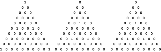
From the branching rules ${\cal A}_{5}\rightarrow{\cal E}_{5}$, we get the following induction rules:

$$\begin{array}[]{ccc}1_{0}\hookleftarrow(0,0),(2,2)&&2_{1}\hookleftarrow(1,0),(2,1),(1,3),(3,2)\\ 1_{1}\hookleftarrow(0,2),(3,2)&&2_{2}\hookleftarrow(0,1),(1,2),(3,1),(2,3)\\ 1_{2}\hookleftarrow(1,2),(5,0)&&2_{3}\hookleftarrow(1,1),(0,3),(2,2),(4,1)\\ 1_{3}\hookleftarrow(3,0),(0,3)&&2_{4}\hookleftarrow(0,2),(2,1),(4,0),(1,3)\\ 1_{4}\hookleftarrow(2,1),(0,5)&&2_{5}\hookleftarrow(2,0),(1,2),(3,1),(0,4)\\ 1_{5}\hookleftarrow(2,0),(2,3)&&2_{0}\hookleftarrow(1,1),(3,0),(2,2),(1,4)\end{array}$$

The same information can be gathered from the columns of matrix $E_{0}$ (see Fig 9: each triangle corresponds to a single column). The first rule can be interpreted as a manifestation of the existence of a non trivial quantum invariant of “degree” $(2,2)$.

4.2.3 Quantum symmetries

For each $1_{i}$, we can verify that the values of $T$ on the two corresponding $(\lambda_{1},\lambda_{2})$ coming from the induction are the same. This allows us to assign a fixed value of T to the $1_{i}$’s. We can also verify that we can not do the same for the other vertices $2_{i}$’s. We get in this way a characterization of the subalgebra $J$, spanned by the elements $1_{i}$’s.

$$\begin{array}[]{|c||c|c|c|c|c|c|c|c|c|c|c|c|}\hline\cr(\lambda_{1},\lambda_{2})&(0,0)&(1,0)&(2,0)&(3,0)&(4,0)&(5,0)&(1,1)&(2,1)&(3,1)&(4,1)&(2,2)&(3,2)\\ &{}\hfil&(0,1)&(0,2)&(0,3)&(0,4)&(0,5)&{}\hfil&(1,2)&(1,3)&(1,4)&{}\hfil&(2,3)\\ \hline\cr\hline\cr\hat{T}&5&1&19&11&1&13&20&13&4&17&5&19\\ \hline\cr\end{array}$$

Table 1: Values of $\hat{T}$ on the vertices of the $\mathcal{A}_{5}$ graph

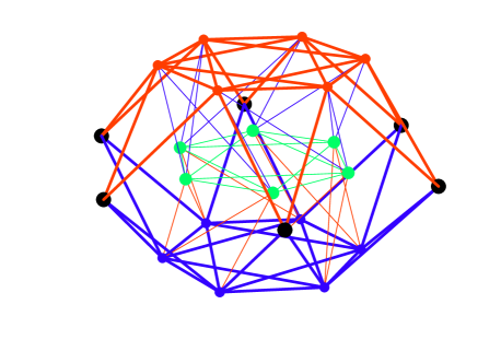
We therefore expect the algebra of quantum symmetries of ${\cal E}_{5}$ to be $Oc({\cal E}_{5})={\cal E}_{5}\otimes_{J}{\cal E}_{5}$. Its dimension is $12.12/6=24$. The left and right subalgebras are respectively spanned by $L=\{a\stackrel{{\scriptstyle\cdot}}{{\otimes}}1_{0}\}$ and $R=\{1_{0}\stackrel{{\scriptstyle\cdot}}{{\otimes}}a\}$, with $a$ equal to $2_{j}$ or $1_{j}$. Both left and right chiral subgraphs have $12$ points. The ambichiral subalgebra (of dimension $6$) is spanned by $A=\{1_{j}\stackrel{{\scriptstyle\cdot}}{{\otimes}}1_{0}=1_{0}\stackrel{{\scriptstyle\cdot}}{{\otimes}}1_{j}\}$ and the supplementary subspace (also $6$ points) is spanned by $C=\{2_{j}\stackrel{{\scriptstyle\cdot}}{{\otimes}}2_{k}=2_{0}\stackrel{{\scriptstyle\cdot}}{{\otimes}}2_{j+k}\}$. The Ocneanu graph can be displayed on the (three dimensional) picture (Fig 10) as two superposed stars kissing each other along the six ambichiral points, with the vertices spanning the supplement displayed “inside” the others. As usual, bold lines — of two different colors — refer to the chiral parts and thin lines to the corresponding quotients. Left chiral graph is blue (bold lines); right chiral graph is red (bold lines). Ambichiral points are black and points belonging to the suppplementary subspace are green. The action of the left generator $2_{1}\stackrel{{\scriptstyle\cdot}}{{\otimes}}1_{0}$ (right generator $1_{0}\stackrel{{\scriptstyle\cdot}}{{\otimes}}2_{1}$) on any point is a linear combination of blue (red) lines. Green lines (bold) are understood as both red and blue thin lines. This graph is oriented but we have not displayed the orientation of the edges in order not to clutter the picture; the interested reader should do it for himself.

Figure 10: Ocneanu graph of ${\cal E}_{5}$

4.2.4 Dimensions of blocks

The two multiplicative structures $\circ$ and $\star$ of the bialgebra ${\cal B}{\cal E}_{5}$ can be diagonalized.
Blocks corresponding to the first structure are labelled by the $21$ points of the ${\cal A}_{5}$ diagram. Dimension $d_{i}$ of the block $i$ is obtained by summing the matrix elements of $F_{i}$. We order the blocks $i=(\lambda,\mu)$ according to the level, i.e., $(\lambda,\mu)<(\lambda^{\prime},\mu^{\prime})$ if $\lambda<\lambda^{\prime}$ or $\lambda=\lambda^{\prime}$ and $\mu<\mu^{\prime}$, and find:

$${\{12\},\{24,24\},\{36,48,36\},\{36,60,60,36\},\{24,48,60,48,24\},\{12,24,36,36,24,12\}}$$

Dimension of the bialgebra is obtained by summing the square of these $21$ integers $d_{i}$: $dim({\cal B}{\cal E}_{5})=29376$. Dimension of the vector space of essential paths (graded by the Young frames of ${\cal A}_{5}$) is $\sum_{i}d_{i}=720$

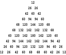
Blocks corresponding to the second structure are labelled by the $24$ points of the Ocneanu graph $Oc({\cal E}_{5})$. Dimension $d_{x}$ of the block $x$ is obtained by summing the matrix elements of matrices $S_{x}=G_{a}G_{b}$ when $x=a\stackrel{{\scriptstyle\cdot}}{{\otimes}}b$ runs over the points of $Oc({\cal E}_{5})$. One finds the following: the $6$ ambichiral blocks have dimension $12$, the six left chiral and the six right chiral blocks which are not ambichiral have dimension $24$, the six complementary blocks have dimension $60$. Dimension of the bialgebra is also obtained by summing the square of these $24$ integers $d_{x}$ and one finds the same total as before. Notice that writing $29376$ in two different ways as a sum of $21$ or $24$ squares constitutes, of course, a rather non trivial check. Notice that we find also $\sum_{x}d_{x}=720$.

We summarize the discussion as follows:

$$dim({\cal B}{\cal E}_{5})=\sum_{i\in{\cal A}_{5}}d_{i}^{2}=\sum_{x\in Oc({\cal E}_{5})}d_{x}^{2}=(2)^{6}(3)^{3}(17)^{1}\quad\text{and}\quad\sum_{i\in{\cal A}_{5}}d_{i}=\sum_{x\in Oc({\cal E}_{5})}d_{x}=(2)^{4}(3)^{2}(5)^{1}$$

4.2.5 Toric matrices and twisted partition functions

From the essential matrices $E_{a}$, we easily calculate the toric matrices (square matrices of dimension $21$) and the corresponding partition functions by the method described earlier. There is one such function for each point of the Ocneanu graph $Oc({\cal E}_{5})$. The one obtained from the identity $1_{0}\stackrel{{\scriptstyle\cdot}}{{\otimes}}1_{0}$ of the graph is the modular-invariant and agrees with the expression of [13] (there is a global shift of $(1,1)$ due to our conventions):

$$\begin{array}[]{lcc}{\cal Z}_{{\cal E}_{5}}\doteq{\cal Z}_{1_{0}\stackrel{{\scriptstyle\cdot}}{{\otimes}}1_{0}}&=&|\chi_{(0,0)}+\chi_{(2,2)}|^{2}+|\chi_{(0,2)}+\chi_{(3,2)}|^{2}+|\chi_{(2,0)}+\chi_{(2,3)}|^{2}\\ {}&+&|\chi_{(2,1)}+\chi_{(0,5)}|^{2}+|\chi_{(3,0)}+\chi_{(0,3)}|^{2}+|\chi_{(1,2)}+\chi_{(5,0)}|^{2}\end{array}$$

The others are interpreted as twisted partition functions (one defect line, in the interpretation of [31]). We give only the twisted partition functions associated with ambichiral points $1_{0}\stackrel{{\scriptstyle\cdot}}{{\otimes}}1_{i}$, for $i\in\{1,2,3,4,5\}$:

$$\begin{array}[]{ccl}{\cal Z}_{1_{0}\stackrel{{\scriptstyle\cdot}}{{\otimes}}1_{1}}&=&(\chi_{(0,3)}+\chi_{(3,0)}).(\overline{\chi}_{(0,5)}+\overline{\chi}_{2,1)})+(\chi_{(2,0)}+\chi_{(2,3)}).(\overline{\chi}_{(0,0)}+\overline{\chi}_{2,2)})+(\chi_{(0,5)}+\chi_{(2,1)}).(\overline{\chi}_{(2,0)}+\overline{\chi}_{2,3)})\\ &+&(\chi_{(1,2)}+\chi_{(5,0)}).(\overline{\chi}_{(0,3)}+\overline{\chi}_{3,0)})+(\chi_{(0,0)}+\chi_{(2,2)}).(\overline{\chi}_{(0,2)}+\overline{\chi}_{3,2)})+(\chi_{(0,2)}+\chi_{(3,2)}).(\overline{\chi}_{(1,2)}+\overline{\chi}_{5,0)})\\ {}\hfil&{}\hfil&{}\\ {\cal Z}_{1_{0}\stackrel{{\scriptstyle\cdot}}{{\otimes}}1_{2}}&=&(\chi_{(1,2)}+\chi_{(5,0)}).(\overline{\chi}_{(0,5)}+\overline{\chi}_{2,1)})+(\chi_{(0,5)}+\chi_{(2,1)}).(\overline{\chi}_{(0,0)}+\overline{\chi}_{2,2)})+(\chi_{(0,3)}+\chi_{(3,0)}).(\overline{\chi}_{(2,0)}+\overline{\chi}_{2,3)})\\ &+&(\chi_{(0,2)}+\chi_{(3,2)}).(\overline{\chi}_{(0,3)}+\overline{\chi}_{3,0)})+(\chi_{(2,0)}+\chi_{(2,3)}).(\overline{\chi}_{(0,2)}+\overline{\chi}_{3,2)})+(\chi_{(0,0)}+\chi_{(2,2)}).(\overline{\chi}_{(1,2)}+\overline{\chi}_{5,0)})\\ {}\hfil&{}\hfil&{}\\ {\cal Z}_{1_{0}\stackrel{{\scriptstyle\cdot}}{{\otimes}}1_{3}}&=&(\chi_{(0,2)}+\chi_{(3,2)}).(\overline{\chi}_{(0,5)}+\overline{\chi}_{2,1)})+(\chi_{(0,3)}+\chi_{(3,0)}).(\overline{\chi}_{(0,0)}+\overline{\chi}_{2,2)})+(\chi_{(1,2)}+\chi_{(5,0)}).(\overline{\chi}_{(2,0)}+\overline{\chi}_{2,3)})\\ &+&(\chi_{(0,0)}+\chi_{(2,2)}).(\overline{\chi}_{(0,3)}+\overline{\chi}_{3,0)})+(\chi_{(0,5)}+\chi_{(2,1)}).(\overline{\chi}_{(0,2)}+\overline{\chi}_{3,2)})+(\chi_{(2,0)}+\chi_{(2,3)}).(\overline{\chi}_{(1,2)}+\overline{\chi}_{5,0)})\\ {}\hfil&{}\hfil&{}\\ {\cal Z}_{1_{0}\stackrel{{\scriptstyle\cdot}}{{\otimes}}1_{4}}&=&(\chi_{(0,0)}+\chi_{(2,2)}).(\overline{\chi}_{(0,5)}+\overline{\chi}_{2,1)})+(\chi_{(1,2)}+\chi_{(5,0)}).(\overline{\chi}_{(0,0)}+\overline{\chi}_{2,2)})+(\chi_{(0,2)}+\chi_{(3,2)}).(\overline{\chi}_{(2,0)}+\overline{\chi}_{2,3)})\\ &+&(\chi_{(2,0)}+\chi_{(2,3)}).(\overline{\chi}_{(0,3)}+\overline{\chi}_{3,0)})+(\chi_{(0,3)}+\chi_{(3,0)}).(\overline{\chi}_{(0,2)}+\overline{\chi}_{3,2)})+(\chi_{(0,5)}+\chi_{(2,1)}).(\overline{\chi}_{(1,2)}+\overline{\chi}_{5,0)})\\ {}\hfil&{}\hfil&{}\\ {\cal Z}_{1_{0}\stackrel{{\scriptstyle\cdot}}{{\otimes}}1_{5}}&=&(\chi_{(2,0)}+\chi_{(2,3)}).(\overline{\chi}_{(0,5)}+\overline{\chi}_{2,1)})+(\chi_{(0,2)}+\chi_{(3,2)}).(\overline{\chi}_{(0,0)}+\overline{\chi}_{2,2)})+(\chi_{(0,0)}+\chi_{(2,2)}).(\overline{\chi}_{(2,0)}+\overline{\chi}_{2,3)})\\ &+&(\chi_{(0,5)}+\chi_{(2,1)}).(\overline{\chi}_{(0,3)}+\overline{\chi}_{3,0)})+(\chi_{(1,2)}+\chi_{(5,0)}).(\overline{\chi}_{(0,2)}+\overline{\chi}_{3,2)})+(\chi_{(0,3)}+\chi_{(3,0)}).(\overline{\chi}_{(1,2)}+\overline{\chi}_{5,0)})\end{array}$$

4.3 Second example: the ${\cal E}_{9}$ case

This diagram is illustrated on Fig 11 (notice that it would be better drawn three-dimensionally as a small starwars spaceship with two wings and a cockpit, because of the existing symmetries between the two wings, reminiscent of what happens for the $D_{2n}$ Dynkin diagrams).

Figure 11: Diagramme de Dynkin généralisé ${\cal E}_{9}$

The corresponding diagram of the $A$ series is ${\cal A}_{9}$. Altitude of both is $\kappa=9+3=12$. Their respective adjacency matrices are immediately read from the graphs. Their number of vertices are $12$ and $10\times 11/2=55$. Restriction and induction is studied as usual, and imposing constancy of the modular operator $T$ singles out the three circled vertices of Fig 11 as elements of the vector subspace $J$ that is used to characterize the ambichiral points of the Ocneanu graph. The fused adjacency matrices $F_{i}$ are obtained from the $su(3)$ recurrence formula; this determines the essential matrices $E_{a}$. We give on Fig 12 the columns of the $E_{0}$ matrix indexed by the three special points (these are the “ambichiral columns” of the intertwiner $E_{0}$); a consistent value of $T$ can be defined for these three points (and these three points only), one finds $\hat{T}=9$ for the vertex $0_{0}$ and $\hat{T}=21$ for $1_{0}$ and $2_{0}$.

Figure 12: Induction corresponding to the three upper vertices of ${\cal E}_{9}$

Blocks of the bialgebra ${\cal B}{\cal E}_{9}$, for its first associative law ($\circ$), are labelled by the $55$ vertices of ${\cal A}_{9}$ and their dimensions are given on Fig 13. The total dimension is the sum of corresponding squares: $dim({\cal B}{\cal E}_{9})=\sum_{i}d_{i}^{2}=518976=(2)^{6}(3)^{2}(17)^{1}(53)^{1}$.

Figure 13: Dimension of space of blocks (law $\circ$ ) for $\mathcal{E}_{9}$

Something special happens however for this graph (again reminiscent of a similar situation in the $D_{2n}$ case of Dynkin diagrams): first of all, the diagram itself is not sufficient to determine a unique associative algebra structure, and one has to impose positivity and integrality of the structure constants in order to determine a self-fusion structure (it is unique up to permutation of the two wings). Since the determination of the corresponding graph matrices is not totally straightforward, we give below the two matrices corresponding to the endpoints $1_{0}$ and $2_{0}$. We choose the following order for the vertices : $0_{0},1_{0},2_{0},3_{0};0_{1},1_{1},2_{1},3_{1};0_{2},1_{2},2_{2},3_{2}$. We also give the adjacency matrix $G_{0_{1}}$ whose determination is straightforward.

$$G_{{0}_{1}}=\left(\begin{array}[]{cccccccccccc}.&.&.&.&.&.&.&.&1&.&.&.\\ .&.&.&.&.&.&.&.&.&1&.&.\\ .&.&.&.&.&.&.&.&.&.&1&.\\ .&.&.&.&.&.&.&.&1&1&1&2\\ 1&.&.&1&.&.&.&.&.&.&.&.\\ .&1&.&1&.&.&.&.&.&.&.&.\\ .&.&1&1&.&.&.&.&.&.&.&.\\ .&.&.&2&.&.&.&.&.&.&.&.\\ .&.&.&.&1&.&.&1&.&.&.&.\\ .&.&.&.&.&1&.&1&.&.&.&.\\ .&.&.&.&.&.&1&1&.&.&.&.\\ .&.&.&.&1&1&1&1&.&.&.&.\\ \end{array}\right)$$

$$G_{{1}_{0}}=\left(\begin{array}[]{cccccccccccc}.&1&.&.&.&.&.&.&.&.&.&.\\ .&.&1&.&.&.&.&.&.&.&.&.\\ 1&.&.&.&.&.&.&.&.&.&.&.\\ .&.&.&1&.&.&.&.&.&.&.&.\\ .&.&.&.&.&1&.&.&.&.&.&.\\ .&.&.&.&.&.&1&.&.&.&.&.\\ .&.&.&.&1&.&.&.&.&.&.&.\\ .&.&.&.&.&.&.&1&.&.&.&.\\ .&.&.&.&.&.&.&.&.&1&.&.\\ .&.&.&.&.&.&.&.&.&.&1&.\\ .&.&.&.&.&.&.&.&1&.&.&.\\ .&.&.&.&.&.&.&.&.&.&.&1\end{array}\right)\quad G_{{2}_{0}}=\left(\begin{array}[]{cccccccccccc}.&.&1&.&.&.&.&.&.&.&.&.\\ 1&.&.&.&.&.&.&.&.&.&.&.\\ .&1&.&.&.&.&.&.&.&.&.&.\\ .&.&.&1&.&.&.&.&.&.&.&.\\ .&.&.&.&.&.&1&.&.&.&.&.\\ .&.&.&.&1&.&.&.&.&.&.&.\\ .&.&.&.&.&1&.&.&.&.&.&.\\ .&.&.&.&.&.&.&1&.&.&.&.\\ .&.&.&.&.&.&.&.&.&.&1&.\\ .&.&.&.&.&.&.&.&1&.&.&.\\ .&.&.&.&.&.&.&.&.&1&.&.\\ .&.&.&.&.&.&.&.&.&.&.&1\end{array}\right)$$

Next, and as expected, the operator $T$ does not distinguish between these two points, and we therefore expect, as in the $D_{2n}$ case of the $su(2)$ system, that the algebra $Oc({\cal E}_{9})$ of quantum symmetries will possess a non-commutative $2\times 2$ matrix component, encoding, in a “non-commutative geometrical spirit”, this indistinguishability. The presence of such a non commutative piece is also reflected in the presence of a coefficient $2$ in the (known) modular invariant partition function. We note, however, that ambichiral points are bound to be, in any case, $0_{0}\stackrel{{\scriptstyle\cdot}}{{\otimes}}0_{0}$, $1_{0}\stackrel{{\scriptstyle\cdot}}{{\otimes}}0_{0}=0_{0}\stackrel{{\scriptstyle\cdot}}{{\otimes}}1_{0}$ and $2_{0}\stackrel{{\scriptstyle\cdot}}{{\otimes}}0_{0}=0_{0}\stackrel{{\scriptstyle\cdot}}{{\otimes}}2_{0}$. The corresponding toric matrices $W$ and partition functions ${\cal Z}$ are computed as usual. We define the linear combination $U$ and $V$ of characters:

$$\begin{array}[]{rcl}U&=&\chi_{(2,2)}+\chi_{(2,5)}+\chi_{(5,2)}\\ V&=&\chi_{(0,0)}+\chi_{(0,9)}+\chi_{(9,0)}+\chi_{(1,4)}+\chi_{(4,1)}+\chi_{(4,4)}\end{array}$$

and find:

$$\begin{array}[]{rcl}{\cal Z}_{0_{0}\stackrel{{\scriptstyle\cdot}}{{\otimes}}0_{0}}&=&2\,U.\overline{U}+V.\overline{V}\\ {\cal Z}_{1_{0}\stackrel{{\scriptstyle\cdot}}{{\otimes}}0_{0}}={\cal Z}_{2_{0}\stackrel{{\scriptstyle\cdot}}{{\otimes}}0_{0}}&=&U.\overline{V}+V.\overline{U}\end{array}$$

The first one is modular invariant and agrees with the expression of Gannon [13]. The other one should be interpreted as a twisted partition function in a BCFT with defect lines.

Unfortunately, in this case, as it was for $D_{2n}$, the data provided by the eigenvalues of the modular operator $T$ does not seem to be sufficient to determine the full (non commutative in this case) structure of $Oc({\cal E}_{9})$ or the Ocneanu graph itself, and we decide to stop at this point.

4.4 Third example: the ${\cal E}_{21}$ case

The ${\cal E}_{21}$ diagram is illustrated in Fig 9. The corresponding ${\cal A}$ diagram with same norm is ${\cal A}_{21}$. The altitude of both is $\kappa=21+3=24$. Their respective adjacency matrices $G_{1}$ and $N_{1}$ are immediately obtained from the diagrams. The number of vertices of the two diagrams are respectively equal to $24$ and $22\times 23/2=253$.

Figure 14: The ${\cal E}_{21}$ generalized Dynkin diagram

4.4.1 Restriction and induction mechanism

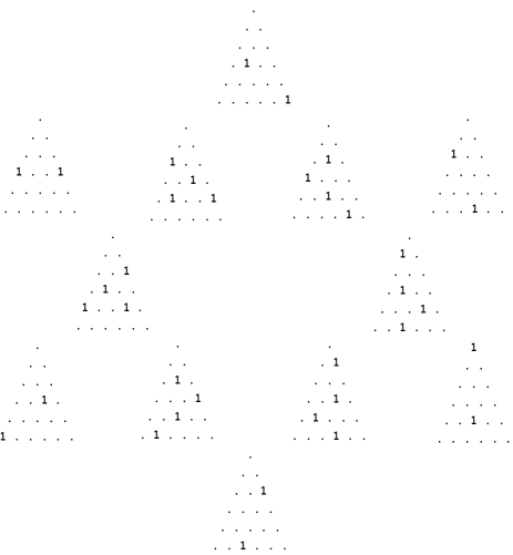
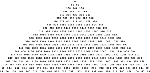
The easiest method is to determine first the fused matrices $F_{i}$ by using the recurrence formula for $su(3)$. Essential matrices $E_{a}$ – and in particular $E_{0}$ – are then obtained in the usual way from the $F_{i}$’s. The first column of $E_{0}$ gives the quantum invariants, it is displayed on the left array of Figure 15.

Figure 15: Induction corresponding to the two extreme points of ${\cal E}_{21}$

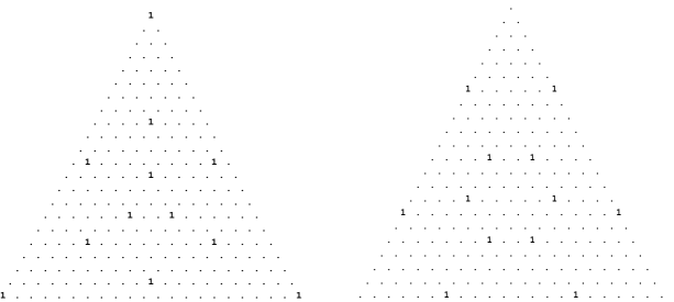
One can check that the values of the modular operator $T$, calculated for ${\cal A}_{21}$, are equal for all non-zero entries of this table. The same property is also true for the column of $E_{0}$ associated with the rightmost point of the ${\cal E}_{21}$ graph (right array of Figure 15). However, $T$, when evaluated on non-zero entries of the $22$ other columns of $E_{0}$, is not constant. We conclude that the set $J$ charactering the ambichiral points of $Oc({\cal E}_{21})$ is a set with two elements: the two extreme vertices of ${\cal E}_{21}$. The values of the modular exponent $\hat{T}$ obtained for these two points are $\hat{T}=21$ and $\hat{T}=39$.

The dimensions $d_{j}$, with $j=(\lambda_{1},\lambda_{2})$ of the $253$ blocks of the bialgebra ${\cal B}{\cal E}_{21}$, for the first law determined by composition of endomorphisms, are obtained by summing matrix elements of matrices $F_{j}$. We obtain: $dim({\cal B}{\cal E}_{21})=\sum_{j}d_{j}^{2}=480701952=(2)^{9}(3)^{4}(67)^{1}(173)^{1}$, and also $\sum_{j}d_{j}=288576=(2)^{6}(3)^{3}(167)^{1}$.

Figure 16: Dimensions of spaces of blocks (law $\circ$)

4.4.2 Determination of the graph algebra and of matrices $G_{a}$

The determination of graph matrices $G_{a}$ comes from the graph ${\cal E}_{21}$ itself. To ease the calculation, it is worth noticing that graph matrices associated with points symmetric with respect to the horizontal symmetry axis of the graph are transposed. We have for example $G_{5}=G_{1}.G_{1}-G_{2}$ so that $G_{4}=(G_{5})^{t}=G_{2}.G_{2}-G_{1}$. Their determination is straightforward from vertices $1$ to $9$. We then use the fact that $G_{6}.G_{21}=G_{9}$ to compute the matrix $G_{21}$ associated with the rightmost point of the graph. Multiplying a vertex $k$ by the vertex $21$ gives a vertex which is the symmetric of $k$ with respect to the center of the graph (the center of a star). In graph algebra terms, we get for example $G_{5}.G_{21}=G_{20}$ and $G_{8}.G_{21}=G_{17}$. It is then easy to compute the matrices associated with all the other vertices of the graph. The most important result, for what follows, is that $G_{21}.G_{21}=G_{0}$.

4.4.3 Quantum symmetries

As already discussed, the subspace $J$ of ${\cal E}_{21}$ determining the algebra of quantum symmetries is spanned by $0$ and $21$; we set $Oc({\cal E}_{21})={\cal E}_{21}\otimes_{J}{\cal E}_{21}$. This is a commutative algebra. The left and right subalgebras $L$ and $R$ are respectively spanned by $a\stackrel{{\scriptstyle\cdot}}{{\otimes}}0$ and by $0\stackrel{{\scriptstyle\cdot}}{{\otimes}}a$, where $a=0,1,\ldots 23$. Both left and right chiral subgraphs have $24$ points. The ambichiral subalgebra $A$, of dimension $2$ is spanned by $\{0\stackrel{{\scriptstyle\cdot}}{{\otimes}}0=21\stackrel{{\scriptstyle\cdot}}{{\otimes}}21\}$ and by $\{0\stackrel{{\scriptstyle\cdot}}{{\otimes}}21=21\stackrel{{\scriptstyle\cdot}}{{\otimes}}0\}$. The supplementary subspace $C$ is spanned by $u\stackrel{{\scriptstyle\cdot}}{{\otimes}}a$, where $u\in\{1,2,3,4,5,6,7,8,10,11,12\}$ and $a$ takes all possible values (but neither $0$ nor $21$). The total number of vertices of the Ocneanu graph is therefore $22+22+2+11\times 22=288$, as expected from the naive dimension count $24\times 24/2=288$. As usual, blocks corresponding to the second structure of the bialgebra ${\cal B}{\cal E}_{21}$ are labelled by the $288$ points of the Ocneanu graph, and the dimension $d_{x}$ of the block $x$ is obtained by summing the matrix elements of matrices $S_{x}=G_{a}G_{b}$ when $x=a\stackrel{{\scriptstyle\cdot}}{{\otimes}}b$ runs over the points of $Oc({\cal E}_{21})$. We find (subscript give multiplicities of the blocks):

$$\begin{array}[]{lcl}\text{Ambichiral}&:&(24)_{2}\\ \text{Left (not ambichiral)}&:&(60)_{4}(108)_{4}(132)_{4}(144)_{2}(168)_{2}(216)_{2}(252)_{4}\\ \text{Right (not ambichiral)}&:&(60)_{4}(108)_{4}(132)_{4}(144)_{2}(168)_{2}(216)_{2}(252)_{4}\\ \text{Supplement}&:&(168)_{8}(312)_{16}(384)_{16}(420)_{8}(492)_{8}(600)_{8}(636)_{8}(744)_{32}(804)_{8}(936)_{8}\\ {}&{}\hfil&(948)_{8}(996)_{8}(1080)_{2}(1188)_{8}(1236)_{8}(1272)_{4}(1440)_{16}(1512)_{2}(1548)_{8}\\ {}&{}\hfil&(1656)_{4}(1800)_{16}(1932)_{8}(1968)_{4}(2292)_{8}(2568)_{2}(2988)_{8}(3480)_{8}\end{array}$$

The quadratic and linear sum rules read:

$$\begin{array}[]{cccclcl}\sum d_{x}&=&\sum d_{i}&=&288576&=&(2)^{6}(3)^{3}(167)^{1}\\ \sum d_{x}^{2}&=&\sum d_{i}^{2}&=&480701952&=&(2)^{9}(3)^{4}(67)^{1}(173)^{1}\end{array}$$

4.4.4 Toric matrices and twisted partition functions

We define the linear combination $U$ and $V$ of characters as follows:

$$\begin{array}[]{ccc}U&=&\chi_{(0,0)}+\chi_{(0,21)}+\chi_{(1,10)}+\chi_{(4,4)}+\chi_{(4,13)}+\chi_{(6,6)}\\ {}\hfil&+&\chi_{(6,9)}+\chi_{(9,6)}+\chi_{(10,1)}+\chi_{(10,10)}+\chi_{(13,4)}+\chi_{(21,0)}\\ V&=&\chi_{(0,6)}+\chi_{(0,15)}+\chi_{(4,7)}+\chi_{(4,10)}+\chi_{(6,0)}+\chi_{(6,15)}\\ {}\hfil&+&\chi_{(7,4)}+\chi_{(7,10)}+\chi_{(10,4)}+\chi_{(10,7)}+\chi_{(15,0)}+\chi_{(15,6)}\end{array}$$

The modular-invariant partition function ${\cal Z}_{{\cal E}_{5}}$ (associated with the vertex $0\stackrel{{\scriptstyle\cdot}}{{\otimes}}0$) and the one associated with the vertex $0\stackrel{{\scriptstyle\cdot}}{{\otimes}}21$, that we call ${\cal Z}_{{\cal E}_{5}}^{{}^{\prime}}$ are:

$$\begin{array}[]{ccccl}{\cal Z}_{{\cal E}_{5}}&\doteq&{\cal Z}_{0\stackrel{{\scriptstyle\cdot}}{{\otimes}}0}&=&U.\overline{U}+V.\overline{V}\\ {\cal Z}_{{\cal E}_{5}}^{{}^{\prime}}&\doteq&{\cal Z}_{0\stackrel{{\scriptstyle\cdot}}{{\otimes}}21}&=&U.\overline{V}+V.\overline{U}\end{array}$$

The first one agrees with the expression of [13], the other, as explained in section 2.2, should be interpreted as a twisted partition function in a BCFT with one defect line [29]. There are $286$ other such functions for the ${\cal E}_{21}$ diagram but these two are the only ones that are ambichiral.

5 Appendices

5.1 About modular invariance

The expressions for $S$ and $T$ can be taken from the theory of quantum groups ${\cal U}_{q}({\cal G})$ at roots of unity, i.e., when $q=e^{\frac{i\pi}{\mu\kappa}}$. Here $\mu$ is half the length of a long root, so it is equal to $1$ when the Lie algebra ${\cal G}$ is simply laced, which is the case in particular for $su(2)$ and $su(3)$, and $\kappa$ is an arbitrary positive integer, larger or equal to $h$, the dual Coxeter number of $\cal G$. The equation $\kappa=h+k$ defines the “level” $k$. One should consider a particular category whose objects are the so-called tilting modules of ${\cal U}_{q}({\cal G})$ and whose morphisms are defined up to “negligible morphisms” (see for instance [1]); this is a semisimple ribbon and modular category. This implies, in particular, that a (projective) representation of $SL(2,\mathbb{Z})$ can be defined on the simple objects, thanks to two matrices $s$ and $t$ and a phase $\zeta$ which are such that $(st)^{3}=\zeta^{3}s^{2}$, $s^{2}=C$, $Ct=tC$ and $C^{2}=1$. The matrix $C$ is called “conjugation matrix” and $t$ is the “modular twist”. For this category, $\zeta=e^{2i\pi c/24}$ with $c=(\kappa-h)dim({\cal G})/\kappa$. The expression for the $t$ matrix, in the case of an arbitrary Lie algebra ${\cal G}$ is $t_{mn}=\delta_{mn}q^{<<n,n+2\rho>>}$ where $\rho$ is half the sum of positive roots and $m$, $n$ are elements of the weight lattice of ${\cal G}$ characterizing the representation $\tau_{m}$ and $\tau_{n}$. Here $<<.,.>>$ is an invariant bilinear form on $\cal G$ normalized by $<<\alpha,\alpha>>=2$ for a short root $\alpha$. The corresponding general expression for the $s$ matrix is more involved and we do not need it in our paper. The same expressions for the modular generators can be obtained from the Kac-Peterson formulae [16] for the modular transformations of characters of the affine Lie algebra $\widehat{\cal G}$, evaluated at the same value $q=e^{\frac{i\pi}{\mu\kappa}}$. Here $k=\kappa-h$ is indeed equal to the usual level.

In the case of $su(2)$, the modular generators $S$, $T$, are as follows: $S=s$ and $T=t/\zeta$. The $SL(2,\mathbb{Z})$ relations read then $(ST)^{3}=S^{2}=1$, with $s_{mn}=\sqrt{\frac{2}{\kappa}}\sin(\pi\frac{(m+1)(n+1)}{\kappa})$, for $0\leq m,n\leq\kappa-2$ and $t_{mn}=e^{\frac{i\pi}{2\kappa}n(n+2)}\delta_{mn}$. Still for $su(2)$ we have $c=3-6/\kappa$, so that $\zeta=e^{i\pi/4}e^{\frac{-i\pi}{2\kappa}}$ and therefore

$$T_{mn}=exp[2i\pi(\frac{(n+1)^{2}}{4\kappa}-\frac{1}{8})]\delta_{mn}$$

which is the expression used in the text. One can explicitly see that the previous $SL(2,\mathbb{Z})$ relations hold. It can be checked, from this expression that, $T^{8\kappa}=1$ when $\kappa$ is odd and $T^{4\kappa}=1$ when $\kappa$ is even. This, by itself, is not enough to imply the following property, which is nevertheless true, and was proven more than a hundred years ago [15]: the above representation of $SL(2,\mathbb{Z})$ factorizes over the finite group $SL(2,\mathbb{Z}/8\kappa\mathbb{Z})$ when $\kappa$ is odd, and factorizes over $SL(2,\mathbb{Z}/4\kappa\mathbb{Z})$ when $\kappa$ is even. So, in particular, $T^{40}=1$ for the $A_{4}$ graph ($40=8\times 5$), but $T^{48}=1$ for the $A_{11}$ graph ($48=4\times 12$). In the text, we use (for $su(2)$) a “modular exponent” defined by $\hat{T}=(n+1)^{2}$ mod $4\kappa$, but it is clear that we could use as well $n(n+2)$ mod $4\kappa$ or any other expression differing by a constant shift.

5.2 The general notion of essential paths on a graph $G$ of type ADE

The following definitions are not needed if we only want to count the number of essential paths on a graph. They are necessary if we want to obtain explicit expressions for them. These definitions are adapted from [23], see also several comments made in [7] and [6]. Call $\beta$ the norm of the graph $G$ (the biggest eigenvalue of its adjacency matrix ${\cal G}$) and $D_{i}$ the components of the (normalized) Perron Frobenius eigenvector. Call $\sigma_{i}$ the vertices of $G$ and, if $\sigma_{j}$ is a neighbour of $\sigma_{i}$, call $\xi_{ij}$ the oriented edge from $\sigma_{i}$ to $\sigma_{j}$. If $G$ is unoriented (the case for $ADE$ and affine $ADE$ diagrams), each edge should be considered as carrying both orientations. An elementary path can be written either as a finite sequence of consecutive (i.e., neighbours on the graph) vertices, $[\sigma_{a_{1}}\sigma_{a_{2}}\sigma_{a_{3}}\ldots]$, or, better, as a sequence $(\xi(1)\xi(2)\ldots)$ of consecutive edges, with $\xi(1)=\xi_{a_{1}a_{2}}=\sigma_{a_{1}}\sigma_{a_{2}}$, $\xi(2)=\xi_{a_{2}a_{3}}=\sigma_{a_{2}}\sigma_{a_{3}}$, etc. . Vertices are considered as paths of length $0$. The length of the (possibly backtracking) path $(\xi(1)\xi(2)\ldots\xi(p))$ is $p$. We call $r(\xi_{ij})=\sigma_{j}$, the range of $\xi_{ij}$ and $s(\xi_{ij})=\sigma_{i}$, the source of $\xi_{ij}$. For all edges $\xi(n+1)=\xi_{ij}$ that appear in an elementary path, we set ${\xi(n+1)}^{-1}\doteq\xi{ji}$. For every integer $n>0$, the annihilation operator $C_{n}$, acting on the vector space generated by elementary paths of length $p$ is defined as follows: if $p\leq n$, $C_{n}$ vanishes, whereas if $p\geq n+1$ then

$$C_{n}(\xi(1)\xi(2)\ldots\xi(n)\xi(n+1)\ldots)=\sqrt{\frac{D_{r(\xi(n))}}{D_{s(\xi(n))}}}\delta_{\xi(n),{\xi(n+1)}^{-1}}(\xi(1)\xi(2)\ldots{\hat{\xi}(n)}{\hat{\xi}(n+1)}\ldots)$$

Here, the symbol “hat” ( like in $\hat{\xi}$) denotes omission. The result is therefore either $0$ or a linear combination of paths of length $p-2$. Intuitively, $C_{n}$ chops the round trip that possibly appears at positions $n$ and $n+1$.

A path is called essential if it belongs to the intersection of the kernels of the anihilators $C_{n}$’s.

Here comes an example of calculation for the $E_{6}$ diagram (square brackets enclose $q$-numbers),

$$C_{3}(\xi_{01}\xi_{12}\xi_{23}\xi_{32}) = \sqrt{\frac{1}{[2]}}(\xi_{01}\xi_{12})$$

$$C_{3}(\xi_{01}\xi_{12}\xi_{25}\xi_{52}) = \sqrt{\frac{[2]}{[3]}}(\xi_{01}\xi_{12})$$

The following difference of non essential paths of length $4$ starting at $\sigma_{0}$ and ending at $\sigma_{2}$ is an essential path of length $4$ on $E_{6}$:

$$\sqrt{[2]}(\xi_{01}\xi_{12}\xi_{23}\xi_{32})-\sqrt{\frac{[3]}{[2]}}(\xi_{01}\xi_{12}\xi_{25}\xi_{52})=\sqrt{[2]}[0,1,2,3,2]-\sqrt{\frac{[3]}{[2]}}[0,1,2,5,2]$$

Remember the values of the $q$-numbers: $[2]=\frac{\sqrt{2}}{\sqrt{3}-1}$ and $[3]=\frac{2}{\sqrt{3}-1}$.

Acting on elementary path of length $p$, the creating operators $C^{{\dagger}}_{n}$ are defined as follows: if $n>p+1$, $C^{{\dagger}}_{n}$ vanishes and, if $n\leq p+1$ then, setting $j=r(\xi(n-1))$,

$$C^{{\dagger}}_{n}(\xi(1)\ldots\xi(n-1)\ldots)=\sum_{d(j,k)=1}\sqrt{(}\frac{D_{k}}{D_{j}})(\xi(1)\ldots\xi(n-1)\xi_{jk}\xi_{kj}\ldots)$$

The above sum is taken over the neighbours $\sigma_{k}$ of $\sigma_{j}$ on the graph. Intuitively, this operator adds one (or several) small round trip(s) at position $n$. The result is therefore either $0$ or a linear combination of paths of length $p+2$. For instance, on paths of length zero (i.e., vertices),

$$C^{{\dagger}}_{1}(\sigma_{j})=\sum_{d(j,k)=1}\sqrt{(}\frac{D_{k}}{D_{j}})\xi_{jk}\xi_{kj}=\sum_{d(j,k)=1}\sqrt{(}\frac{D_{k}}{D_{j}})\,[\sigma_{j}\sigma_{k}\sigma_{j}]$$

Jones’ projectors $e_{k}$ can be realized (as endomorphisms of $Path^{p}$) by

$$e_{k}\doteq\frac{1}{\beta}C^{{\dagger}}_{k}C_{k}$$

The reader can check that all Jones-Temperley-Lieb relations between the $e_{i}$ are satisfied. Essential paths can also be defined as elements of the intersection of the kernels of the Jones projectors $e_{i}$’s.

5.3 The structure of $\mathcal{B}G$

Paths on $G$ generate a vector space $Paths(G)$ which comes with a grading: paths of homogeneous grade $j$ are associated with Young diagrams of $SU(N)$. In the case of $su(2)$ this grading is just an integer (to be thought of as a length or as a point of a diagram of type ${\cal A}$).

What turns out to be most interesting is a particular vector subspace $\mathcal{E}=EssPaths(G)$ of $Paths$ whose elements are called “essential paths” (see above definition). This subspace is is itself graded in the same way as $Paths$.

We then consider the graded algebra of endomorphisms of essential paths

$$\mathcal{B}G=End_{\sharp}(EssPaths)=\bigoplus_{j=0,r-1}End(EssPaths^{j})$$

which, by definition, is an associative algebra. By using the fact that paths on the chosen diagram can be concatenated, one may define [23] another multiplicative associative structure on $\mathcal{B}G$ that we call convolution product (see our comments in the next subsection). This vector space with two algebra structures is called, by A. Ocneanu, the “Algebra of double triangles”.

Existence of a scalar product allows one to transmute one of the multiplications (for instance the convolution product) into a co-multiplication and it happens that the coproduct $\Delta$ is compatible with the product (in the sense that we have the homomorphism property $\Delta(uv)=\Delta u\otimes\Delta v$). $\mathcal{B}G$ is therefore a bialgebra. However, $\mathcal{B}G$ is not a Hopf algebra but a weak Hopf algebra (or quantum groupoid). This statement should be taken with a grain of salt: see our comments in the next subsection. General axioms for weak Hopf algebras are given in [3]. In the present case, the following axiom for Hopf algebras fails to be satisfied: the coproduct of the unit $\Delta\mbox{\rm 1}\hskip-2.8pt\mbox{\rm l}=\mbox{\rm 1}\hskip-2.8pt\mbox{\rm l}_{1}\otimes\mbox{\rm 1}\hskip-2.8pt\mbox{\rm l}_{2}$ is not equal to $\mbox{\rm 1}\hskip-2.8pt\mbox{\rm l}\otimes\mbox{\rm 1}\hskip-2.8pt\mbox{\rm l}$ (as usual, a summation is understood); several other axioms for Hopf algebras are also modified: the counit is not an homomorphism ($\epsilon(xy)=\epsilon(x\mbox{\rm 1}\hskip-2.8pt\mbox{\rm l}_{1})\epsilon(y\mbox{\rm 1}\hskip-2.8pt\mbox{\rm l}_{2})$) and, if $\Delta^{2}x=x_{1}\otimes x_{2}\otimes x_{3}$, the compatibility axiom for the antipode is modified as follows $S(x_{1})x_{2}\otimes x_{3}=\mbox{\rm 1}\hskip-2.8pt\mbox{\rm l}_{1}\otimes x\mbox{\rm 1}\hskip-2.8pt\mbox{\rm l}_{2}$.

5.4 Remarks and open questions

Essential paths for $ADE$ diagrams (i.e., the $su(2)$ system) have been defined in several published papers but their analogues for higher systems (for instance the Di Francesco - Zuber diagrams), although reasonably well understood by a few people, have never been described, as far as we know, in the litterature.

The general definition of the convolution product of $\mathcal{B}G$, for $ADE$ diagrams, was given “explicitly” by A. Ocneanu in [23] by a rather difficult formula involving several types of generalized quantum $6j$ symbols. It is certainly interesting to know this general formula, but, in our opinion, this expression is not very helpful for a practical investigation of the different cases.

The fact that $\mathcal{B}G$ is a weak Hopf algebra is a claim that belongs to the folklore, but we are not aware of any general reference showing that all the axioms of [3] are indeed verified in this situation. The authors (together with A. Garcia and R. Trinchero) have however checked that it is so in a number of particular cases belonging to the ADE series and are working on a general proof.

Another possibility for defining the convolution product of $\mathcal{B}G$ is to make use of the notion of cell systems. This general notion was defined in [22]; it is also described in [12] and it is used, in a particular context by [32]. We cannot summarize this theory here. Let us just mention that a cell system involves four graphs (top, bottom, left and right) with matching properties and that, in the present case, the top and bottom graphs are the same $ADE$ diagram $G$. Cells are rectangles with top and bottom edges which are also edges of the given graph(s). Macrocells have top and bottom edges (or “horizontal paths”) that coïncide with the essential paths on $G$; their left and right edges are called “vertical paths”. To every cell system one can associate “‘connections” which are particular maps associating complex numbers with cells or macrocells. These numbers, in turn, can be used to define the structure constants of the algebra we are looking for. For every point of the graph $Oc(G)$ there is an irreducible connection on the cell system (or an irreducible quantum symmetry). Although it seems to provide (at the time of this writing) the shortest road to the explicit construction of the bialgebra $\mathcal{B}G$, this construction is unfortunately not explicitely available in the litterature.

Among other results, and in the framework of statistical mechanics, the paper [31] gives many useful relations between the vertical product of $\mathcal{B}G$ (the product of endomorphisms acting on $EssPaths(G)$) and its horizontal product (or convolution product). There are indeed several families of numeral constants that appear as structure constants for these two products, or that appear as coefficients of a kind of Fourier transform relating the two. These constants look like generalized quantum 6j symbols and obey different types of (mixed) pentagon equations which themselves generalize the quantum group version of the Biedenharn - Elliot identity. As discussed in [3], any solution of this “Big Pentagon Equation” (involving six different types of generalized $6j$ symbols) determines the structural maps of a weak $C^{*}$ Hopf algebra. Unfortunately, we do not know a single reference that describes a practical implementation of this general construction (and gives the values of these structure constants) for the bialgebras $\mathcal{B}G$ associated with specific $ADE$ diagrams or with their higher generalizations.

Graphs $Oc(G)$, encoding the structure of the algebra of quantum symmetries of the diagram $G$, have been “conceptually” defined by A. Ocneanu in terms of the block structure of $\mathcal{B}G$ for its convolution product, but it is interesting to notice that, to our knowledge, they were never obtained in this way…Clearly, it would be interesting to do so. We repeat that our modest purpose, in the present paper, was to observe that known Ocneanu graphs (or algebras), in the ADE cases, could be recovered, in most cases, from the modular properties of the $T$ matrix; we then used this observation to study several cases belonging to the $su(3)$ system. The problem of deducing Ocneanu graphs from the explicit structure of the bialgebra $\mathcal{B}G$, in the different cases, is a much more difficult and interesting program that it would be nice to investigate.

Here comes a short list of open questions that, we hope, may trigger the interest of the reader:

• Give a simple definition – valid in all cases – of the convolution product of $\mathcal{B}G$.

• Show that this bialgebra is indeed a weak Hopf algebra in all cases.

• Is it possible to find a kind of multiplication on $EssPaths(G)$ that would allow one to construct $\mathcal{B}G$ in a functorial (and simple) way ?

• Determine explicitly the graphs $Oc(G)$ directly from the study of the corresponding bialgebra $\mathcal{B}G$.

• Find a simple algorithm allowing one to calculate all irreducible connections on cell systems (i.e., the values of cells) in all $ADE$ or generalized $ADE$ cases.

• Precise the relation (if any) between the generalized Coxeter-Dynkin systems and the finite subgroups of Lie groups.

• What is the interpretation of all these contructions in terms of the finite dimensional Hopf quotients of $U_{q}(SL2)$ at roots of unity ?

• Can one, in some sense, “supersymmetrize” these constructions ?

• What is the origin of the linear sum rules ?

• What is the origin of the quantum sum rules ?

• As we know, toric matrices (twisted or not) described in the text can be interpreted as partition functions (with or without defect lines) on a torus, at the critical point, for affine models (WZW models). Clearly this framework can be generalized in several directions: one may consider more general correlation functions, replace affine models by (generalized) minimal models, replace the torus by higher genus surfaces…

• We know explicitly how to generalize the $ADE$ diagrams in the cases of $su(3)$ and $su(4)$ and a definition of what are the “generalized Coxeter-Dynkin systems” was briefly mentionned in [24] but a detailed description of this notion is clearly needed.

• What kind of algebraic structures (generalizing the notion of Lie algebras) can one associate with a diagram belonging to such a generalized system ?

References

- [1] B. Bakalov, A. Kirillov Jr., Lectures on tensor categories and modular functors, AMS, Univ. Lect. Notes Series Vol.21(2001).
- [2] J. Böckenhauer and D. Evans, Modular invariants, graphs and induction for nets of subfactors II, Commun. Math. Phys. 197, 361-386(1998), 200, 57-103(1999), 205, 183-228200(1999).
- [3] G. Böhm, K. Szlachanyi, A coassociative -quantum group with non-integral dimensions, Lett. Math. Phys. 38 (1996) no 4, 437-456, q-alg/9509008.
- [4] A.Cappelli, C.Itzykson and J.B. Zuber, The ADE classification of minimal and conformal invariant theories, Comm. Math. Phys. 13(1987)1.
- [5] C. H. Otto Chui, C. Mercat, W. Orrick and P. A. Pearce, Integrable Lattice Realizations of Conformal Twisted Boundary Conditions, hep-th/0106182.
- [6] R. Coquereaux, Classical and quantum polyhedra: A fusion graph algebra point of view, AIP Conference Proceedings 589 (2001), 37th Karpacz Winter School of Theor. Phys., J. Lukierski and J. Rembielinski eds, 181-203, hep-th/0105239.
- [7] R. Coquereaux, Notes on the quantum tetrahedron, Moscow Math. J. vol2, n1, Jan.-March 2002, 1-40, hep-th/0011006.
- [8] R. Coquereaux, G. Schieber, Twisted partition functions for boundary conformal field theories and Ocneanu algebras of quantum symmetries, J. of Geom. and Phys. 781 (2002), 1-43, hep-th/0107001.
-
[9]
P. Di Francesco, J.-B. Zuber, in Recent Developments in Conformal Field
Theories, Trieste Conference 1989, S. Randjbar-Daemi, E Sezgin and J.-B. Zuber eds,
World Scientific 1990;
P. Di Francesco, Int. J. Mod. Phys. A7 (1992) 407-500. - [10] P.Di Francesco, P. Matthieu, D. Senechal, Conformal Field Theory (Springer, 1997).
- [11] F. Di Francesco, J.-B. Zuber, SU(N) Lattice integrable models associated with graphs, Nucl. Phys B338 (1990) 602-646.
- [12] : D. Evans and Y. Kawahigashi, Quantum symmetries and operator algebras, Clarendon Press, 1998.
- [13] T. Gannon, The Classification of affine su(3) modular invariants, Comm. Math. Phys. 161, 233-263 (1994).
- [14] F.M. Goodman, P. de la Harpe and V.F.R Jones, Coxeter graphs and towers of algebras, MSRI publications 14 (Springer, 1989).
- [15] A. Hurwitz, Über endliche Gruppen, welche in der Theory der elliptischen Transzendenten autraten; Math. Annalen 27, (1886), 183-233.
- [16] V.G. Kac and D.H. Peterson, Infinite dimensional Lie algebras, theta functions and modular forms, Adv in Maths. 53 (1984), no 2, 125-264.
- [17] A. Kirillov Jr. and V. Ostrik, On q-analog of McKay correspondence and classification of conformal field theories, math.QA/0101219.
- [18] F. Klein, Lectures on the Icosahedron and the solution of the equation of the fifth degree, Reprog. Nachdr. d. Ausg. Leipzig (1884), Teubner. Dover Pub, New York, Inc IX, 289p (1956).
[19]
I. Kostov, Nucl. Phys. B300 (1988) 559;
P. Fendley, P. Ginsparg, Nucl. Phys. B324 (1989) 549;
P. Fendley, New exactly solvable models, J. Phys. A22 (1989) 4633. - [20] J. McKay, Graphs, singularities and finite groups, Proc. Symp. Pure Math. 37(1980)183.
- [21] D. Nikshych, L. Vainerman, Finite Quantum Groupoïds and Their Applications, math.QA/0006057.
- [22] A. Ocneanu; Quantized groups, string algebras and Galois theory for algebras. Warwick (1987), in Operator algebras and applications, Lond Math Soc Lectures note Series 136, CUP (1988).
[23]
A. Ocneanu, Paths on Coxeter
diagrams: from Platonic solids and singularities to minimal models
and subfactors, Talks given at the Centre de Physique Théorique,
Luminy, Marseille, 1995.
Same title: notes taken by S. Goto, Fields Institute Monographs (Rajarama Bhat et al eds, AMS, 1999). -
[24]
A. Ocneanu, Higher Coxeter systems, Talk given at
MSRI,
http://www.msri.org/publications/ln/msri/2000/subfactors/ocneanu. - [25] A. Ocneanu, The Classification of subgroups of quantum SU(N), Lectures at Bariloche Summer School, Argentina, Jan.2000, AMS Contemporary Mathematics 294, R. Coquereaux, A. García and R. Trinchero eds.
- [26] V. Ostrik, Module categories, weak Hopf algebras, and modular invariance, math.QA/0111139.
- [27] V. Pasquier, Operator contents of the ADE lattice models, J. Phys A20 (1987) 5707.
- [28] V. Pasquier, Two-dimensional critical systems labeled by Dynkin diagrams, Nucl.Phys. B 285(1987)162.
[29]
V.B. Petkova and J.-B. Zuber, Generalized
twisted partition functions, Phys. Lett. B 504
(1-2)(2001)157, hep-th/0011021. - [30] V.B. Petkova and J.-B. Zuber, Conformal Field Theories, Graphs and Quantum Algebras, in MATHPHYS ODYSSEY2001, M. Kashiwara and T. Miwa eds, Progress in Math., Birkhauser, hep-th/0108236.
- [31] V.B. Petkova and J.-B. Zuber, The many faces of Ocneanu cells, Nucl. Phys. B 603(2001)449, hep-th/0101151.
- [32] Ph. Roche, Ocneanu cell calculus and integrable lattice models, Comm.Math.Phys. 127(1990)395.
[33]
P. Slodowy, A new A-D-E classification,
Bayreuther Mathematische Schriften 33 (1990),
197-213. -
[34]
E. Verlinde, Fusion rules and modular transformations in 2-D Conformal
Field Theory,
Nucl. Phys. B300: 360-376 (1988). - [35] J.-B. Zuber, Graphs algebras, conformal field theories and integrable models, Nucl. Phys. B (Proc. Supplement) 18B (1990), 313-326.
- [36] J.-B. Zuber, Generalized Dynkin diagrams and root systems and their foldings, Proc. of the Tanigushi Symposium, Kyoto, Dec. 1996, hep-th/9708046.
- [37] J.-B. Zuber, Graphs and reflection graphs, Comm. Math. Phys. 179 (1996) 265-294.
- [38] J.-B. Zuber, CFT, BCFT, and all that, Lectures at Bariloche Summer School, Argentina, Jan 2000, AMS Contemporary Mathematics 294, R. Coquereaux, A. García and R. Trinchero eds, hep-th/0006151.