Zeeman Spectroscopy of the Star Algebra

Abstract:

We solve the problem of finding all eigenvalues and eigenvectors of the Neumann matrix of the matter sector of open bosonic string field theory, including the zero modes, and switching on a background $B$-field. We give the discrete eigenvalues as roots of transcendental equations, and we give analytical expressions for all the eigenvectors.

1 Introduction

After Rastelli, Sen and Zwiebach calculated, in [1], the spectrum and all the eigenvectors of the zero-momentum Neumann matrix in the matter sector $M$, it has become clear that the knowledge of the spectrum is very useful to perform exact calculations in string field theory [2, 3, 4]. Also, it has recently been shown by Douglas, Liu, Moore and Zwiebach in [5] that this allows us to write the star-product of two zero-momentum string fields as a continuous tensor product of Moyal products, each of which corresponding to one eigenvalue in the spectrum of $M$. The noncommutativity parameter $\theta$ of each of these Moyal products is given as a function of the eigenvalue $\lambda$. For $\lambda=-{1\over 3}$, it is zero, and we therefore have one commutative product corresponding to the momentum carried by half of a string (which is conserved in this setup).

Because of this success, it has become a subject of interest to diagonalize Neumann matrices in diverse situations: In [6], Mariño and Schiappa diagonalized the Neumann matrices of superstring field theory. In a recent paper [7] we diagonalized $M^{\prime}$, the bosonic Neumann matrix in the matter sector including zero modes; the same work was done independently by Belov [8]. We found that the spectrum of $M^{\prime}$ has the same continuous part as that of $M$, that is the interval $[-{1\over 3},0)$, plus one doubly degenerate eigenvalue in the range $(0,1)$, whose value depends on the parameter $b$, defined by $a_{0}={1\over 2}\sqrt{b}\hat{p}-{1\over\sqrt{b}}i\hat{x}$.

The goal of this paper is to diagonalize the Neumann matrix ${\cal M}^{11}$ with zero modes in a nontrivial $B$-field background. The form of the star-product in the presence of a $B$-field was already studied in [9, 10, 11, 12, 13]. We will use here the formalism of Bonora, Mamone and Salizzoni [13] for the Neumann matrix ${\cal M}^{11}$ with nonzero $B$-field, which we can easily cast into the form introduced by Okuyama [3]. Therefore, it is merely an extension of our work [7] to give complete expressions for the eigenvalues and eigenvectors of ${\cal M}^{11}$.

In short, our results are as follows: We turn on a $B$-field $\left(\begin{array}[]{cc}0&B\\ -B&0\end{array}\right)$ in two spatial directions. First we find a scaling parameter $\xi=1+(2\pi\alpha^{\prime}B)^{2}$, such that our continuous spectrum is $[-{1\over 3\xi},0)$, the same as that of $M$ or $M^{\prime}$ but shrunk by $\xi$. Each eigenvalue in this interval is four times degenerate (they are twice more degenerate than the eigenvalues of $M^{\prime}$ simply because we are considering two spatial directions instead of a single one), except the point $\lambda=-{1\over 3\xi}$ which is only doubly degenerate when $B\neq 0$. Then we find two doubly degenerate discrete eigenvalues in the range $(0,{1\over\xi})$ (again the same range as for $M^{\prime}$ but shrunk by $\xi$). We give these two eigenvalues in terms of roots of transcendental equations depending on $b$ and $B$. When $B=0$, these eigenvalues are the same, whereas the role of turning on a $B$-field is just to split them and push one eigenvalue towards $0$ and the other one towards ${1\over\xi}$ (This is reminiscent of the Zeeman effect). Finally we give analytical expressions for all the eigenvectors.

This paper is organized as follows. We begin with nomenclature and some review of the known results in diagonalising the Neumann matrix, especially with the zero modes, in Section 2. Then in Section 3 we proceed to the basic setup of diagonalising the matrix in the presence of a $B$-field background. Here we reduce the problem to the solution of a $4\times 4$ linear system. We next address the case of the continuous spectrum in Section 4. Thereafter we focus on the properties of the determinant of the $4\times 4$ system in Section 5 so as to obtain a discrete spectrum in Section 6. To verify our analysis, we perform level truncation analysis in Section 7 and come to satisfying agreement. We end with conclusions and prospects in Section 8.

2 Notations and Some Review of Known Results

In a previous work [7], we generalised the results of [1, 2, 3] in studying the spectrum of the Neumann Matrix by including the zero mode. We recall that this is the matrix

$$M^{\prime}:=\left(\begin{array}[]{cc}M^{\prime}_{00}&M^{\prime}_{0m}\\ M^{\prime}_{n0}&M^{\prime}_{nm}\end{array}\right)=\left(\begin{array}[]{ll}1-\frac{2}{3}\frac{b}{\beta}&-\frac{2}{3}\frac{\sqrt{2b}}{\beta}\left\langle v_{e}\right|{}{}{}{}{}{}{}\\ -\frac{2}{3}\frac{\sqrt{2b}}{\beta}\left|v_{e}\right\rangle&M+\frac{4}{3}\frac{(-\left|v_{e}\right\rangle\left\langle v_{e}\right|+\left|v_{o}\right\rangle\left\langle v_{0}\right|)}{\beta}\end{array}\right),$$

with

$$\beta:=V_{00}^{rr}+\frac{b}{2}=\ln\frac{27}{16}+\frac{b}{2},\qquad\begin{array}[]{l}\left|v_{e}\right\rangle:=E^{-1}\left|A_{e}\right\rangle\\ \left|v_{o}\right\rangle:=E^{-1}\left|A_{o}\right\rangle,\end{array}\quad E_{mn}:=\sqrt{n}\delta_{mn}$$

and

$$\begin{array}[]{l}(A_{e})_{n}:=\frac{1+(-)^{n}}{2}A_{n}\\ (A_{o})_{n}:=\frac{1-(-)^{n}}{2}A_{n},\end{array}\quad\mbox{s.t.}~{}~{}(\frac{1+ix}{1-ix})^{1/3}:=\sum_{n=even}A_{n}x^{n}+i\sum_{n=odd}A_{n}x^{n}.$$

Now we recall that $M^{\prime}$ has a continuous spectrum in $[-1/3,0)$ with eigenvalue $M(k)=-\frac{1}{1+2\cosh\frac{\pi k}{2}}$, with a pair of degenerate twist-even and twist-odd eigenvalues under the twist operator $C_{mn}:=(-1)^{m}\delta_{mn}$. Moreover, $M^{\prime}$ has an isolated eigenvalue inside $(0,1)$ also with doubly degenerate eigenvectors.

We shall also adhere to the following definitions, as in [7]. All the vectors will ultimately be written in the basis

$$\left|k\right\rangle=(v_{1}^{k},v_{2}^{k},v_{3}^{k},...)^{T}$$

with the generating function

$$f_{k}(z)=\sum_{n=1}^{+\infty}\frac{v_{n}^{k}}{\sqrt{n}}z^{n}=\frac{1}{k}(1-e^{-k\arctan z}).$$

Defining $|z\rangle=(z,z^{2},z^{3},...)^{T}$, and the inner product

$$\langle z\left|k\right\rangle\equiv\sum_{n=1}^{+\infty}z^{n}v_{n}^{k},$$

we have orthonormality and closure conditions:

$$\langle k|p\rangle={\cal N}(k)\delta(k-p),\qquad{\cal N}(k):=\frac{2}{k}\sinh(\frac{\pi k}{2});\quad{\bf 1}=\int_{-\infty}^{+\infty}dk\frac{\left|k\right\rangle\left\langle k\right|}{{\cal N}(k)}.$$

Moreover under the twist action,

$$C\left|z\right\rangle=\left|-z\right\rangle,\qquad C\left|k\right\rangle=-\left|-k\right\rangle.$$

The $\left|v_{e}\right\rangle$ and $\left|v_{o}\right\rangle$ vectors above obey

$$\left\langle k\right|v_{e}\rangle=\frac{1}{k}\frac{\cosh(\frac{\pi k}{2})-1}{2\cosh(\frac{\pi k}{2})+1},~{}~{}~{}~{}\left\langle k\right|v_{o}\rangle=\frac{\sqrt{3}}{k}\frac{\sinh(\frac{\pi k}{2})}{2\cosh(\frac{\pi k}{2})+1}$$

and

$$C\left|v_{e}\right\rangle=\left|v_{e}\right\rangle,\qquad C\left|v_{o}\right\rangle=-\left|v_{o}\right\rangle.$$

Finally, with the inner product the generating functions can be written as

$$f_{k}(z)=\left\langle z\right|E^{-1}\left|k\right\rangle=\langle k|E^{-1}\left|z\right\rangle,$$

and we define also

$$G_{e}(z)\equiv\left\langle z\right|E^{-1}\frac{1}{\lambda-M}\left|v_{e}\right\rangle=\int_{-\infty}^{+\infty}dk{f_{k}(z)\left\langle k\right|v_{e}\rangle\over{\cal N}(k)(\lambda-M(k))},$$

$$G_{o}(z)\equiv\left\langle z\right|E^{-1}\frac{1}{\lambda-M}\left|v_{o}\right\rangle=\int_{-\infty}^{+\infty}dk{f_{k}(z)\left\langle k\right|v_{o}\rangle\over{\cal N}(k)(\lambda-M(k))},$$

whose explicit integrations were carried out in Equations (7.6) and (7.10) of [7].

2.1 The Presence of the Background $B$-Field

Now let us consider the presence of a background field $B^{\alpha\beta}$. We use the notation in [13]. The authors define the following matrices

$$G^{\alpha\beta}=({1\over\eta+2\pi\alpha^{\prime}B}\eta{1\over\eta-2\pi\alpha^{\prime}B})^{\alpha\beta},~{}~{}~{}~{}\theta^{\alpha\beta}=-(2\pi\alpha^{\prime})^{2}({1\over\eta+2\pi\alpha^{\prime}B}B{1\over\eta-2\pi\alpha^{\prime}B})^{\alpha\beta},$$ (1)

where they have chosen the simplest but easily generalizable case of $B$ non-vanishing in two directions ${\alpha\beta}$ equaling to, say 24 and 25, and $\eta^{\alpha\beta}$ is the flat metric in ${\bf R}^{2}$.

Adhering to their convention, we explicitly chose

$$B_{\alpha\beta}=\left(\begin{array}[]{cc}0&B\\ -B&0\end{array}\right),~{}~{}~{}~{}~{}~{}\eta_{\alpha\beta}=\left(\begin{array}[]{cc}1&0\\ 0&1\end{array}\right).$$ (2)

From (2) we can simplify (1) to

$$G^{\alpha\beta}={1\over\xi}\left(\begin{array}[]{cc}1&0\\ 0&1\end{array}\right),~{}~{}~{}~{}~{}\theta^{\alpha\beta}\equiv\theta\epsilon^{\alpha\beta}={-(2\pi\alpha^{\prime})^{2}B\over\xi}\left(\begin{array}[]{cc}0&1\\ -1&0\end{array}\right),$$ (3)

where we have defined

$$\xi=1+(2\pi\alpha^{\prime}B)^{2},~{}~{}~{}~{}\theta={-(2\pi\alpha^{\prime})^{2}B\over\xi}.$$

These immediately give us

$$\det(G)=\xi^{2},\qquad\theta\sqrt{\det(G)}=-(2\pi\alpha^{\prime})^{2}B.$$

For later usage and recalling $\beta:=V_{00}^{rr}+{b\over 2}$, we define two matrices

$$\chi^{rs}=\left(\begin{array}[]{ccc}0&1&-1\\ -1&0&1\\ 1&-1&0\end{array}\right),~{}~{}~{}~{}~{}~{}\phi^{rs}=\left(\begin{array}[]{ccc}1&-{1\over 2}&-{1\over 2}\\ -{1\over 2}&1&-{1\over 2}\\ -{1\over 2}&-{1\over 2}&1\end{array}\right),$$ (4)

as well as two parametres

$$\Omega={2\beta\over 4\pi^{4}{\alpha^{\prime}}^{2}B^{2}+3\beta^{2}},~{}~{}~{}~{}~{}\Xi={i(\pi\alpha^{\prime})^{2}B\over\beta\xi}.$$ (5)

We shall henceforth take $\alpha^{\prime}=1$.

Using these notations we can write the Neumann coefficients in the presence of the background $B$-field [13]: First the vertex is

$$|V_{3}\rangle=\int d^{26}p_{(1)}d^{26}p_{(2)}d^{26}p_{(3)}\delta^{(26)}(p_{(1)}+p_{(2)}+p_{(3)})\exp(-E)|0,p\rangle_{123}\,,$$ (6)

where $E=E_{\|}+E_{\perp}$ is split into a parallel part (for the directions in which $B=0$) which is the same as the vertex without $B$-field, and a perpendicular part (for the two spatial directions in which we switched on the $B$-field) which depends on $B$; it can be written

$$E_{\perp}=\sum_{r,s=1}^{3}\left({1\over 2}\sum_{m,n\geq 1}G_{\alpha\beta}a_{m}^{(r)\alpha\dagger}V_{mn}^{rs}a_{n}^{(s)\beta\dagger}+\sum_{n\geq 1}G_{\alpha\beta}p_{(r)}^{\alpha}V_{0n}^{rs}a_{n}^{(s)\beta\dagger}+{1\over 2}G_{\alpha\beta}p_{(r)}^{\alpha}V_{00}^{rs}p_{(s)}^{\beta}+{i\over 2}\sum_{r<s}p_{\alpha}^{(r)}\theta^{\alpha\beta}p_{\beta}^{(s)}\right)\,.$$ (7)

Here we notice that if we don’t include the zero-modes in our analysis, (7) would simply reduce to

$$\sum_{r,s=1}^{3}\left({1\over 2}\sum_{m,n\geq 1}G_{\alpha\beta}a_{m}^{(r)\alpha\dagger}V_{mn}^{rs}a_{n}^{(s)\beta\dagger}\right)\,.$$

We thus see immediately, from the form of $G_{\alpha\beta}={1\over\xi}\eta_{\alpha\beta}$ in (3), that in this case, the effect of $B$ is just to shrink the spectrum by $\xi$. We will thus include the zero-modes in our analysis. In this case, we write the vertex $|V_{3}\rangle=|V_{3,\perp}\rangle\otimes|V_{3,\|}\rangle$, where $|V_{3,\|}\rangle$ is the same as in the case without $B$-field and $|V_{3,\perp}\rangle=Ke^{-E}|\Omega\rangle$ where $|\Omega\rangle$ is annihilated by all $a_{m}$, $m\geq 0$, $K$ is some constant which depends on $b$ and $B$ [13], and $E$ is

$$E={1\over 2}\sum_{r,s=1}^{3}\sum_{m,n\geq 0}a_{m}^{(r)\alpha\dagger}{\cal V}_{mn}^{\alpha\beta,rs}a_{n}^{(s)\beta\dagger}\,,$$

where

$${\cal V}^{\alpha\beta,rs}_{00} = G^{\alpha\beta}\delta^{rs}-\Omega b(G^{\alpha\beta}\phi^{rs}+\Xi\epsilon^{\alpha\beta}\chi^{rs}),$$ (8)

$${\cal V}^{\alpha\beta,rs}_{0n} = \Omega\sqrt{b}\sum_{t=1}^{3}(G^{\alpha\beta}\phi^{rt}+\Xi\epsilon^{\alpha\beta}\chi^{rt})V_{0n}^{ts},$$ (9)

$${\cal V}^{\alpha\beta,rs}_{mn} = G^{\alpha\beta}V_{mn}^{rs}-\Omega\sum_{t,v=1}^{3}V_{m0}^{rv}(G^{\alpha\beta}\phi^{vt}+\Xi\epsilon^{\alpha\beta}\chi^{vt})V_{0n}^{ts}\,.$$ (10)

These coefficients satisfy the properties

$${\cal V}^{\alpha\beta,rs}_{mn}={\cal V}^{\beta\alpha,sr}_{nm},~{}~{}~{}~{}~{}{\cal V}^{\alpha\beta,rs}_{mn}={\cal V}^{\alpha\beta,(r+1)(s+1)}_{mn}\,.$$

To write these coefficients into a more compact form, we need to invoke from Appendix B [14] the following forms for the Neumann Coefficients, rewritten in our basis:

$$\begin{array}[]{cclccl}V_{n0}^{rr}&=&{-2\sqrt{2}\over 3}\left|v_{e}\right\rangle,&V_{0n}^{rr}&=&{-2\sqrt{2}\over 3}\left\langle v_{e}\right|,\\ V_{n0}^{21}&=&{\sqrt{2}\over 3}\left|v_{e}\right\rangle+{\sqrt{6}\over 3}\left|v_{o}\right\rangle,&V_{0n}^{12}&=&{\sqrt{2}\over 3}\left\langle v_{e}\right|+{\sqrt{6}\over 3}\left\langle v_{o}\right|,\\ V_{n0}^{12}&=&{\sqrt{2}\over 3}\left|v_{e}\right\rangle-{\sqrt{6}\over 3}\left|v_{o}\right\rangle,&V_{0n}^{21}&=&{\sqrt{2}\over 3}\left\langle v_{e}\right|-{\sqrt{6}\over 3}\left\langle v_{o}\right|.\end{array}$$

Substituting the above, (8), (9) and (10) simplify to

$$({\cal V}^{\alpha\beta}_{mn})^{11} = G^{\alpha\beta}[V_{mn}^{11}-2\Omega(\left|v_{e}\right\rangle\left\langle v_{e}\right|+\left|v_{o}\right\rangle\left\langle v_{o}\right|)]$$

$$- {4\over\sqrt{3}}\Omega\Xi\epsilon^{\alpha\beta}[\left|v_{e}\right\rangle\left\langle v_{o}\right|-\left|v_{o}\right\rangle\left\langle v_{e}\right|],$$

$$({\cal V}^{\alpha\beta}_{0n})^{11} = -\sqrt{2b}\Omega G^{\alpha\beta}\left\langle v_{e}\right|-{2\sqrt{6b}\over 3}\Omega\Xi\epsilon^{\alpha\beta}\left\langle v_{o}\right|,$$

$$({\cal V}^{\alpha\beta}_{n0})^{11} = ({\cal V}^{\beta\alpha}_{0n})^{11}$$

$$= -\sqrt{2b}\Omega G^{\alpha\beta}\left|v_{e}\right\rangle+{2\sqrt{6b}\over 3}\Omega\Xi\epsilon^{\alpha\beta}\left|v_{o}\right\rangle,$$

$$({\cal V}^{\alpha\beta}_{00})^{11} = G^{\alpha\beta}(1-\Omega b),$$

We can define two matrices

$$\Gamma := \left(\begin{array}[]{ll}1-\Omega b&-\sqrt{2b}\Omega\left\langle v_{e}\right|\\ -\sqrt{2b}\Omega\left|v_{e}\right\rangle{}{}{}&V^{11}-2\Omega(\left|v_{e}\right\rangle\left\langle v_{e}\right|+\left|v_{o}\right\rangle\left\langle v_{o}\right|)\end{array}\right)$$ (13)

$$\Sigma := \left(\begin{array}[]{ll}0&-{2\sqrt{6b}\over 3}\Omega\Xi\left\langle v_{o}\right|\\ {2\sqrt{6b}\over 3}\Omega\Xi\left|v_{o}\right\rangle{}{}{}&-{4\over\sqrt{3}}\Omega\Xi[\left|v_{e}\right\rangle\left\langle v_{o}\right|-\left|v_{o}\right\rangle\left\langle v_{e}\right|]\end{array}\right)$$ (16)

to simplify things further.

Using (16) we can finally write down the Neumann coefficients $({\cal V})^{11}$ in the presence of the $B$-Field into a $4\times 4$ matrix form

$$({\cal V})^{11}=\left(\begin{array}[]{ll}{1\over\xi}\Gamma&\Sigma\\ -\Sigma&{1\over\xi}\Gamma\end{array}\right)$$ (17)

2.2 The Matrix of Our Concern: $({\cal M})^{11}$

Combining all of the notation above, the matrix we wish to diagonalize is $({\cal V})^{11}$ multiplied by the twist operator $C$, i.e.,

$$({\cal M})^{11}\equiv C({\cal V})^{11}=\left(\begin{array}[]{ll}{1\over\xi}C\Gamma&C\Sigma\\ -C\Sigma&{1\over\xi}C\Gamma\end{array}\right)$$ (18)

where

$$C\Gamma:=\left(\begin{array}[]{ll}1-\Omega b&-\sqrt{2b}\Omega\left\langle v_{e}\right|\\ -\sqrt{2b}\Omega\left|v_{e}\right\rangle{}{}{}&M-2\Omega(\left|v_{e}\right\rangle\left\langle v_{e}\right|-\left|v_{o}\right\rangle\left\langle v_{o}\right|)\end{array}\right)$$

and

$$C\Sigma:=\left(\begin{array}[]{ll}0&-{2\sqrt{6b}\over 3}\Omega\Xi\left\langle v_{o}\right|\\ -{2\sqrt{6b}\over 3}\Omega\Xi\left|v_{o}\right\rangle{}{}{}&-{4\over\sqrt{3}}\Omega\Xi\left(\left|v_{e}\right\rangle\left\langle v_{o}\right|+\left|v_{o}\right\rangle\left\langle v_{e}\right|\right)\end{array}\right).$$

Note that since $\Xi$ from (5) is a purely imaginary number, $({\cal M})^{11}$ is Hermitian, so its eigenvalues are real. It is the diagonalisation of this matrix $({\cal M})^{11}$ with which we shall concern ourselves in the remainder of the paper.

3 Diagonalising $({\cal M})^{11}$: The Setup

Now we can solve the eigenvectors and eigenvalues, as what we did in [7], with the ansatz

$$v=\left(\begin{array}[]{c}g_{1}\\ \int dkh_{1}(k)\left|k\right\rangle\\ g_{2}\\ \int dkh_{2}(k)\left|k\right\rangle\end{array}\right)$$

Acting on $v$ by (18), we can write the eigen-equation into four parts as

$$\lambda g_{1} = {1-\Omega b\over\xi}g_{1}-{\sqrt{2b}\Omega\over\xi}{\cal C}^{(1)}_{e}-{2\sqrt{6b}\over 3}\Omega\Xi{\cal C}^{(2)}_{o},$$

$$\int_{-\infty}^{+\infty}dk\lambda h_{1}(k)\left|k\right\rangle = -{\sqrt{2b}\Omega\over\xi}\left|v_{e}\right\rangle g_{1}+\int_{-\infty}^{+\infty}dk{M(k)\over\xi}h_{1}(k)\left|k\right\rangle-{2\Omega\over\xi}[\left|v_{e}\right\rangle{\cal C}^{(1)}_{e}-\left|v_{o}\right\rangle{\cal C}^{(1)}_{o}]$$

$$- {2\sqrt{6b}\over 3}\Omega\Xi\left|v_{o}\right\rangle g_{2}-{4\over\sqrt{3}}\Omega\Xi[\left|v_{e}\right\rangle{\cal C}^{(2)}_{o}+\left|v_{o}\right\rangle{\cal C}^{(2)}_{e}],$$

$$\lambda g_{2} = {2\sqrt{6b}\over 3}\Omega\Xi{\cal C}^{(1)}_{o}+{1-\Omega b\over\xi}g_{2}-{\sqrt{2b}\Omega\over\xi}{\cal C}^{(2)}_{e},$$

$$\int_{-\infty}^{+\infty}dk\lambda h_{2}(k)\left|k\right\rangle = {2\sqrt{6b}\over 3}\Omega\Xi\left|v_{o}\right\rangle g_{1}+{4\over\sqrt{3}}\Omega\Xi[\left|v_{e}\right\rangle{\cal C}^{(1)}_{o}+\left|v_{o}\right\rangle{\cal C}^{(1)}_{e}]-{\sqrt{2b}\Omega\over\xi}\left|v_{e}\right\rangle g_{2}$$ (19)

$$+ \int_{-\infty}^{+\infty}dk{M(k)\over\xi}h_{2}(k)\left|k\right\rangle-{2\Omega\over\xi}[\left|v_{e}\right\rangle{\cal C}^{(2)}_{e}-\left|v_{o}\right\rangle{\cal C}^{(2)}_{o}]$$

where we have defined

$${\cal C}^{(1)}_{e} = \int_{-\infty}^{+\infty}dkh_{1}(k)\left\langle v_{e}\right|k\rangle,$$

$${\cal C}^{(1)}_{o} = \int_{-\infty}^{+\infty}dkh_{1}(k)\langle v_{o}|k\rangle,$$

$${\cal C}^{(2)}_{e} = \int_{-\infty}^{+\infty}dkh_{2}(k)\left\langle v_{e}\right|k\rangle,$$

$${\cal C}^{(2)}_{o} = \int_{-\infty}^{+\infty}dkh_{2}(k)\langle v_{o}|k\rangle.$$

Now we solve $g_{1},g_{2}$ from the first and third equations of (19):

$$g_{1} = [-{\sqrt{2b}\Omega\over\xi}{\cal C}^{(1)}_{e}-{2\sqrt{6b}\over 3}\Omega\Xi{\cal C}^{(2)}_{o}]/(\lambda-{1-\Omega b\over\xi}),$$

$$g_{2} = [{2\sqrt{6b}\over 3}\Omega\Xi{\cal C}^{(1)}_{o}-{\sqrt{2b}\Omega\over\xi}{\cal C}^{(2)}_{e}]/(\lambda-{1-\Omega b\over\xi}).$$

Putting these back into the second and fourth equations of (19) we obtain

$$\int_{-\infty}^{+\infty}dkh_{1}(k)\left|k\right\rangle[\lambda-{M(k)\over\xi}] = \left|v_{e}\right\rangle[{\cal C}^{(1)}_{e}d_{ee}+{\cal C}^{(2)}_{o}d_{oe}]+\left|v_{o}\right\rangle[{\cal C}^{(1)}_{o}d_{oo}+{\cal C}^{(2)}_{e}d_{oe}]$$

$$\int_{-\infty}^{+\infty}dkh_{2}(k)\left|k\right\rangle[\lambda-{M(k)\over\xi}] = \left|v_{o}\right\rangle[{\cal C}^{(2)}_{o}d_{oo}-{\cal C}^{(1)}_{e}d_{oe}]+\left|v_{e}\right\rangle[{\cal C}^{(2)}_{e}d_{ee}-{\cal C}^{(1)}_{o}d_{oe}],\qquad$$ (20)

where to simplify notation, we have defined

$$d_{ee} = -{2\Omega(\xi\lambda-1)\over\xi(\xi\lambda-1+\Omega b)},$$

$$d_{oo} = {-2\Omega\over 3\xi}[-3+{4b\Omega\Xi^{2}\xi^{2}\over\xi\lambda-1+\Omega b}],$$

$$d_{oe} = -{4\Omega\Xi(\xi\lambda-1)\over\sqrt{3}(\xi\lambda-1+\Omega b)}.$$

We note that $d_{ee},d_{oo}$ are reals while $d_{oe}$ is purely imaginary.

We can expand $\left|v_{e}\right\rangle,\left|v_{o}\right\rangle$ as in (4.7) of [7]

$$\left|v_{e}\right\rangle=\int_{-\infty}^{+\infty}dk\left|k\right\rangle\frac{\left\langle k\right|v_{e}\rangle}{{\cal N}(k)},\qquad\left|v_{o}\right\rangle=\int_{-\infty}^{+\infty}dk\left|k\right\rangle\frac{\left\langle k\right|v_{o}\rangle}{{\cal N}(k)}.$$

Subsequently, (20) can be re-written as

$$h_{1}(k) = {1\over\lambda-{M(k)\over\xi}}[{\langle k|v_{e}\rangle\over{\cal N}(k)}(d_{ee}{\cal C}^{(1)}_{e}+d_{oe}{\cal C}^{(2)}_{o})+{\langle k|v_{o}\rangle\over{\cal N}(k)}(d_{oo}{\cal C}^{(1)}_{o}+d_{oe}{\cal C}^{(2)}_{e})+\delta(k-k_{1})r_{1}(k)],$$

$$h_{2}(k) = {1\over\lambda-{M(k)\over\xi}}[{\langle k|v_{e}\rangle\over{\cal N}(k)}(d_{ee}{\cal C}^{(2)}_{e}-d_{oe}{\cal C}^{(1)}_{o})+{\langle k|v_{o}\rangle\over{\cal N}(k)}(d_{oo}{\cal C}^{(2)}_{o}-d_{oe}{\cal C}^{(1)}_{e})+\delta(k-k_{2})r_{2}(k)]$$ (21)

with yet undetermined parameters $k_{1},k_{2}$ and functions $r_{1}(k),r_{2}(k)$ with zeros respectively at $k_{1},k_{2}$. Again, as in [7], we define

$$A_{ee}(\lambda) = \int_{-\infty}^{+\infty}dk\frac{\left\langle k\right|v_{e}\rangle\langle v_{e}\left|k\right\rangle}{{\cal N}(k)(\lambda-{M(k)\over\xi})}=\left\langle v_{e}\right|\frac{1}{\lambda-{M\over\xi}}\left|v_{e}\right\rangle,$$

$$A_{eo}(\lambda) = \int_{-\infty}^{+\infty}dk\frac{\left\langle k\right|v_{o}\rangle\langle v_{e}\left|k\right\rangle}{{\cal N}(k)(\lambda-{M(k)\over\xi})}=\left\langle v_{e}\right|\frac{1}{\lambda-{M\over\xi}}\left|v_{o}\right\rangle=0,$$

$$A_{oo}(\lambda) = \int_{-\infty}^{+\infty}dk\frac{\left\langle k\right|v_{o}\rangle\langle v_{o}\left|k\right\rangle}{{\cal N}(k)(\lambda-{M(k)\over\xi})}=\left\langle v_{o}\right|\frac{1}{\lambda-{M\over\xi}}\left|v_{o}\right\rangle,$$

$$B_{e}^{(1)}(\lambda) = \int_{-\infty}^{+\infty}dk\frac{\delta(k-k_{1})r_{1}(k)\langle v_{e}\left|k\right\rangle}{\lambda-{M(k)\over\xi}},$$

$$B_{o}^{(1)}(\lambda) = \int_{-\infty}^{+\infty}dk\frac{\delta(k-k_{1})r_{1}(k)\langle v_{o}\left|k\right\rangle}{\lambda-{M(k)\over\xi}},$$

$$B_{e}^{(2)}(\lambda) = \int_{-\infty}^{+\infty}dk\frac{\delta(k-k_{2})r_{2}(k)\langle v_{e}\left|k\right\rangle}{\lambda-{M(k)\over\xi}},$$

$$B_{o}^{(2)}(\lambda) = \int_{-\infty}^{+\infty}dk\frac{\delta(k-k_{2})r_{2}(k)\langle v_{o}\left|k\right\rangle}{\lambda-{M(k)\over\xi}}.$$ (22)

Finally, we can write the eigen-equation (19) we wish to solve into matrix form:

$$\left(\begin{array}[]{cccc}1-d_{ee}A_{ee}{}{}&0&0&-d_{oe}A_{ee}\\ 0&1-d_{oo}A_{oo}{}{}&-d_{oe}A_{oo}&0\\ 0&d_{oe}A_{ee}&1-d_{ee}A_{ee}{}{}&0\\ d_{oe}A_{oo}&0&0&1-d_{oo}A_{oo}\end{array}\right)\left(\begin{array}[]{l}{\cal C}^{(1)}_{e}\\ {\cal C}^{(1)}_{o}\\ {\cal C}^{(2)}_{e}\\ {\cal C}^{(2)}_{o}\end{array}\right)=\left(\begin{array}[]{l}B^{(1)}_{e}\\ B^{(1)}_{o}\\ B^{(2)}_{e}\\ B^{(2)}_{o}\end{array}\right).$$ (23)

To solve this equation we need to consider the determinant $Det$ of the $4\times 4$ matrix in (23). We will leave this discussion to section 5. For now let us address the case when $Det\neq 0$ so that we can invert (23); this gives us the continuous spectrum.

4 The Continuous Spectrum

As we will see from Section 5, only a few $\lambda$’s make the determinant zero. For other $\lambda$, the determinant is non-zero and we can invert to solve ${\cal C}$’s. Just as what we did in [7], to get the nonzero solution, $\lambda$ must be in the region ${1\over\xi}[-1/3,0)$. This is what is going to give us the continuous spectrum.

4.1 The Continuous Eigenvalues

To see the above discussion more clearly, let us write down the explicit form of $B_{e}$ from (22):

$$B_{e}^{(1)}=\int_{-\infty}^{+\infty}dk\frac{1}{k}\frac{\cosh(\frac{\pi k}{2})-1}{2\cosh(\frac{\pi k}{2})+1}\frac{\delta(k-k_{1})r_{1}(k)}{\lambda-{M(k)\over\xi}},$$

Since $r_{1}(k_{1})=0$, the above integration will be zero unless the denominator $\lambda-{M(k)\over\xi}$ also has a zero at $k=k_{1}$:

$$\lambda-{M(k_{1})\over\xi}=0\,.$$

Because $M(k_{1})\in[-1/3,0)$ for any $k_{1}$, we know immediately that we have a continuous spectrum for any

$$\lambda={M(k)\over\xi}\in{1\over\xi}[-1/3,0);$$ (24)

this is our continuous eigenvalue. Comparing with the result in [7] we see that in the background of $B$, the continuous spectrum is simply scaled by a factor of ${1\over\xi}$.

4.2 The Continuous Eigenvectors

Now let us construct the eigenvector for the given $\lambda$ from (24) but not equal to ${-1\over 3\xi}$. We will consider this special point in Subsection 4.3.

Now let us set

$$\lambda={M(k_{0})\over\xi}=-\frac{1}{\xi}\frac{1}{1+2\cosh\frac{\pi k_{0}}{2}}$$ (25)

for our eigenvalue from (24). we expand $\lambda-M(k)/\xi$ around $k_{0}$ as

$$\lambda-{M(k)\over\xi} = {1\over\xi}[M(k_{0})-M(k)]={1\over\xi}[-\frac{dM}{dk}|_{k_{0}}(k-k_{0})-\frac{1}{2}\frac{d^{2}M}{dk^{2}}|_{k_{0}}(k-k_{0})^{2}+....]$$

$$= {1\over\xi}[-\frac{\pi\sinh\frac{\pi k_{0}}{2}}{(1+2\cosh\frac{\pi k_{0}}{2})^{2}}(k-k_{0})-\frac{1}{2}\frac{\pi^{2}+\frac{\pi^{2}}{2}\cosh\frac{\pi k_{0}}{2}-\pi^{2}\sinh^{2}\frac{\pi k_{0}}{2}}{(1+2\cosh\frac{\pi k_{0}}{2})^{3}}(k-k_{0})^{2}+....]$$

Recall that we have two independent pairs of parameters $(k_{1},r_{1}(k))$ and $(k_{2},r_{2}(k))$ with $r_{i}(k_{i})=0$. We freely choose $k_{1}=k_{2}=k_{0}$, $r_{1}(k)=D_{1}\cdot(k-k_{0})$ and $r_{1}(k)=D_{2}\cdot(k-k_{0})$, where $D_{i=1,2}$ are arbitrary constants. Then we have

$$B_{e}^{(1)} = -\frac{\xi D_{1}(\cosh(\frac{\pi k_{0}}{2})-1)(2\cosh(\frac{\pi k_{0}}{2})+1)}{\pi k_{0}\sinh\frac{\pi k_{0}}{2}}:=B_{e,k_{0}}D_{1},$$

$$B_{o}^{(1)} = -\sqrt{3}\frac{\xi D_{1}(2\cosh(\frac{\pi k_{0}}{2})+1)}{\pi k_{0}}:=B_{o,k_{0}}D_{1},$$

$$B_{e}^{(2)} = -\frac{\xi D_{2}(\cosh(\frac{\pi k_{0}}{2})-1)(2\cosh(\frac{\pi k_{0}}{2})+1)}{\pi k_{0}\sinh\frac{\pi k_{0}}{2}}:=B_{e,k_{0}}D_{2},$$

$$B_{o}^{(2)} = -\sqrt{3}\frac{\xi D_{2}(2\cosh(\frac{\pi k_{0}}{2})+1)}{\pi k_{0}}:=B_{o,k_{0}}D_{2}.$$ (26)

From this we can solve

$$\left(\begin{array}[]{l}{\cal C}^{(1)}_{e}\\ {\cal C}^{(1)}_{o}\\ {\cal C}^{(2)}_{e}\\ {\cal C}^{(2)}_{o}\end{array}\right) = {1\over\Delta}\left(\begin{array}[]{l}(1-d_{oo}A_{oo})B_{e}^{(1)}+d_{oe}A_{ee}B_{o}^{(2)}\\ (1-d_{ee}A_{ee})B_{o}^{(1)}+d_{oe}A_{oo}B_{e}^{(2)}\\ -d_{oe}A_{ee}B_{o}^{(1)}+(1-d_{oo}A_{oo})B_{e}^{(2)}\\ -d_{oe}A_{oo}B_{e}^{(1)}+(1-d_{ee}A_{ee})B_{o}^{(2)}\end{array}\right)$$

$$= {D_{1}\over\Delta}\left(\begin{array}[]{l}(1-d_{oo}A_{oo})B_{e,k_{0}}\\ (1-d_{ee}A_{ee})B_{o,k_{0}}\\ -d_{oe}A_{ee}B_{o,k_{0}}\\ -d_{oe}A_{oo}B_{e,k_{0}}\end{array}\right)+{D_{2}\over\Delta}\left(\begin{array}[]{l}d_{oe}A_{ee}B_{o,k_{0}}\\ d_{oe}A_{oo}B_{e,k_{0}}\\ (1-d_{oo}A_{oo})B_{e,k_{0}}\\ (1-d_{ee}A_{ee})B_{o,k_{0}}\end{array}\right)$$

where we have defined

$$\Delta:=(1-d_{ee}A_{ee})(1-d_{oo}A_{oo})+d_{oe}^{2}A_{ee}A_{oo}$$

so that $\Delta^{2}=Det$.

Now recalling that we can solve the $h_{i}$ from (21) from the ${\cal C}$’s and the $g_{i}$ as well; whence substituting back into (19), we obtain the eigenvector. We see that the general solutions are just the linear combinations of the $D_{1}$ and $D_{2}$ terms:

$$v(k_{0}) = {D_{1}\over\Delta}\left(\begin{array}[]{l}-{\sqrt{2b}\Omega\over(\lambda\xi-1+\Omega b)}(1-d_{oo}A_{oo})B_{e,k_{0}}+{2\sqrt{6b}\Omega\Xi\xi\over 3(\lambda\xi-1+\Omega b)}d_{oe}A_{oo}B_{e,k_{0}}\\ \\ {B_{e,k_{0}}(d_{ee}-(d_{ee}d_{oo}+d_{oe}^{2})A_{oo})\over\lambda-{M\over\xi}}\left|v_{e}\right\rangle+{B_{o,k_{0}}(d_{oo}-(d_{ee}d_{oo}+d_{oe}^{2})A_{ee})\over\lambda-{M\over\xi}}\left|v_{o}\right\rangle-{\xi\Delta\over\frac{dM}{dk}|_{k_{0}}}\left|k_{0}\right\rangle\\ \\ {2\sqrt{6b}\Omega\Xi\xi\over 3(\lambda\xi-1+\Omega b)}(1-d_{ee}A_{ee})B_{o,k_{0}}+{\sqrt{2b}\Omega\over(\lambda\xi-1+\Omega b)}d_{oe}A_{ee}B_{o,k_{0}}\\ \\ {-d_{oe}B_{o,k_{0}}\over\lambda-{M\over\xi}}\left|v_{e}\right\rangle+{-d_{oe}B_{e,k_{0}}\over\lambda-{M\over\xi}}\left|v_{o}\right\rangle\end{array}\right)+$$ (36)

$$+ {D_{2}\over\Delta}\left(\begin{array}[]{l}-{\sqrt{2b}\Omega\over(\lambda\xi-1+\Omega b)}d_{oe}A_{ee}B_{o,k_{0}}-{2\sqrt{6b}\Omega\Xi\xi\over 3(\lambda\xi-1+\Omega b)}(1-d_{ee}A_{ee})B_{o,k_{0}}\\ \\ {d_{oe}B_{o,k_{0}}\over\lambda-{M\over\xi}}\left|v_{e}\right\rangle+{d_{oe}B_{e,k_{0}}\over\lambda-{M\over\xi}}\left|v_{o}\right\rangle\\ \\ {2\sqrt{6b}\Omega\Xi\xi\over 3(\lambda\xi-1+\Omega b)}d_{oe}A_{oo}B_{e,k_{0}}-{\sqrt{2b}\Omega\over(\lambda\xi-1+\Omega b)}(1-d_{oo}A_{oo})B_{e,k_{0}}\\ \\ {B_{e,k_{0}}(d_{ee}-(d_{ee}d_{oo}+d_{oe}^{2})A_{oo})\over\lambda-{M\over\xi}}\left|v_{e}\right\rangle+{B_{o,k_{0}}(d_{oo}-(d_{ee}d_{oo}+d_{oe}^{2})A_{ee})\over\lambda-{M\over\xi}}\left|v_{o}\right\rangle-{\xi\Delta\over\frac{dM}{dk}|_{k_{0}}}\left|k_{0}\right\rangle\end{array}\right)$$ (44)

Since for a given $\lambda$ there are two corresponding $k$-values in solving (25), viz., $k_{0}$ and $-k_{0}$, we get two degenerate states $v(k_{0}),v(-k_{0})$ (in fact, the degeneracy is four because for each we have one corresponding to $D_{1}$ and another to $D_{2}$). Using

$$B_{e,k_{0}}=B_{e,-k_{0}},~{}~{}~{}~{}~{}B_{o,k_{0}}=-B_{o,-k_{0}},~{}~{}~{}~{}~{}~{}\frac{dM}{dk}|_{k_{0}}=-\frac{dM}{dk}|_{-k_{0}}$$

we can write the eigenstates which are even and odd with respect to $k_{0}$:

$$v_{1,\lambda}={v(k_{0})+v(-k_{0})\over 2} = {D_{1}\over\Delta}\left(\begin{array}[]{l}-{\sqrt{2b}\Omega\over(\lambda\xi-1+\Omega b)}(1-d_{oo}A_{oo})B_{e,k_{0}}+{2\sqrt{6b}\Omega\Xi\xi\over 3(\lambda\xi-1+\Omega b)}d_{oe}A_{oo}B_{e,k_{0}}\\ \\ {B_{e,k_{0}}(d_{ee}-(d_{ee}d_{oo}+d_{oe}^{2})A_{oo})\over\lambda-{M\over\xi}}\left|v_{e}\right\rangle-{\xi\Delta\over 2\frac{dM}{dk}|_{k_{0}}}(\left|k_{0}\right\rangle-\left|-k_{0}\right\rangle)\\ \\ 0\\ \\ {-d_{oe}B_{e,k_{0}}\over\lambda-{M\over\xi}}\left|v_{o}\right\rangle\end{array}\right)$$ (52)

$$+ {D_{2}\over\Delta}\left(\begin{array}[]{l}0\\ \\ {d_{oe}B_{e,k_{0}}\over\lambda-{M\over\xi}}\left|v_{o}\right\rangle\\ \\ {2\sqrt{6b}\Omega\Xi\xi\over 3(\lambda\xi-1+\Omega b)}d_{oe}A_{oo}B_{e,k_{0}}-{\sqrt{2b}\Omega\over(\lambda\xi-1+\Omega b)}(1-d_{oo}A_{oo})B_{e,k_{0}}\\ \\ {B_{e,k_{0}}(d_{ee}-(d_{ee}d_{oo}+d_{oe}^{2})A_{oo})\over\lambda-{M\over\xi}}\left|v_{e}\right\rangle-{\xi\Delta\over 2\frac{dM}{dk}|_{k_{0}}}(\left|k_{0}\right\rangle-\left|-k_{0}\right\rangle)\end{array}\right)$$ (60)

$$\equiv {D_{1}\over\Delta}\,v^{e}_{1,\lambda}+{D_{2}\over\Delta}\,v^{o}_{1,\lambda}$$ (61)

and

$$v_{2,\lambda}={v(k_{0})-v(-k_{0})\over 2} = {D_{1}\over\Delta}\left(\begin{array}[]{l}0\\ \\ {B_{o,k_{0}}(d_{oo}-(d_{ee}d_{oo}+d_{oe}^{2})A_{ee})\over\lambda-{M\over\xi}}\left|v_{o}\right\rangle-{\xi\Delta\over 2\frac{dM}{dk}|_{k_{0}}}(\left|k_{0}\right\rangle+\left|-k_{0}\right\rangle)\\ \\ {2\sqrt{6b}\Omega\Xi\xi\over 3(\lambda\xi-1+\Omega b)}(1-d_{ee}A_{ee})B_{o,k_{0}}+{\sqrt{2b}\Omega\over(\lambda\xi-1+\Omega b)}d_{oe}A_{ee}B_{o,k_{0}}\\ \\ {-d_{oe}B_{o,k_{0}}\over\lambda-{M\over\xi}}\left|v_{e}\right\rangle\end{array}\right)$$ (69)

$$+ {D_{2}\over\Delta}\left(\begin{array}[]{l}-{\sqrt{2b}\Omega\over(\lambda\xi-1+\Omega b)}d_{oe}A_{ee}B_{o,k_{0}}-{2\sqrt{6b}\Omega\Xi\xi\over 3(\lambda\xi-1+\Omega b)}(1-d_{ee}A_{ee})B_{o,k_{0}}\\ \\ {d_{oe}B_{o,k_{0}}\over\lambda-{M\over\xi}}\left|v_{e}\right\rangle\\ \\ 0\\ \\ {B_{o,k_{0}}(d_{oo}-(d_{ee}d_{oo}+d_{oe}^{2})A_{ee})\over\lambda-{M\over\xi}}\left|v_{o}\right\rangle-{\xi\Delta\over 2\frac{dM}{dk}|_{k_{0}}}(\left|k_{0}\right\rangle+\left|-k_{0}\right\rangle)\end{array}\right)$$ (77)

$$\equiv {D_{1}\over\Delta}\,v^{o}_{2,\lambda}+{D_{2}\over\Delta}\,v^{e}_{2,\lambda}\,.$$ (78)

However, we see that $v_{i,\lambda}$ are neither twist-even nor twist-odd under the $C$-operator. The twist-even (odd) states in the first direction of our 2-dimensions chosen for the $B$-field are mixed with the twist-odd (even) states in the second direction. This behaviour is of course a result of turning on the background $B$-field.

4.3 The Special Case of $\lambda=-1/(3\xi)$

Now, as promised, we discuss the special case of $\lambda=-1/(3\xi)$ which was excluded from the above. For general $B\neq 0$, $\lambda=-1/(3\xi)$ does not make the determinant zero. Then we can solve the equation as before and find the coefficients ${\cal C}$ and subsequently the eigenvector.

However, one thing is special for this point: this is that $\frac{dM}{dk}|_{k_{0}=0}$ when $k_{0}=0$. In another words, we should choose $r(k)=D\cdot k^{2}$ instead of the linear $r(k)=D\cdot(k-k_{0})$. Under such a choice, we have $B_{e,0}=0$ and $B_{o,0}=-6\sqrt{3}\xi/\pi$. So the solution is

$$v(k_{0}) = {\xi D_{1}\over\Delta}\left(\begin{array}[]{l}0\\ {B_{o,0}(d_{oo}-(d_{ee}d_{oo}+d_{oe}^{2})A_{ee})\over-1/3-M}\left|v_{o}\right\rangle-{36\Delta\over\pi^{2}}\left|0\right\rangle\\ {2\sqrt{6b}\Omega\Xi\xi\over 3\xi(\lambda\xi-1+\Omega b)}(1-d_{ee}A_{ee})B_{o,0}+{\sqrt{2b}\Omega\over\xi(\lambda\xi-1+\Omega b)}d_{oe}A_{ee}B_{o,0}\\ {-d_{oe}B_{o,0}\over-1/3-M}\left|v_{e}\right\rangle\end{array}\right)+$$ (83)

$$+ {\xi D_{2}\over\Delta}\left(\begin{array}[]{l}-{\sqrt{2b}\Omega\over\xi(\lambda\xi-1+\Omega b)}d_{oe}A_{ee}B_{o,0}-{2\sqrt{6b}\Omega\Xi\xi\over 3\xi(\lambda\xi-1+\Omega b)}(1-d_{ee}A_{ee})B_{o,0}\\ \\ {d_{oe}B_{o,0}\over-1/3-M}\left|v_{e}\right\rangle\\ 0\\ {B_{o,0}(d_{oo}-(d_{ee}d_{oo}+d_{oe}^{2})A_{ee})\over-1/3-M}\left|v_{o}\right\rangle-{36\Delta\over\pi^{2}}\left|0\right\rangle\end{array}\right).$$ (89)

Now at $k_{0}=0$ we get only two independent eigenvectors instead of the four as discussed at the end of the last subsection. This may seem a little surprising because when $B=0$, we do have four eigenvectors (since we have two spatial directions instead of one in [7]: two of $v_{+,-{1\over 3}}$ and two of $v_{-,-{1\over 3}}$). However, after a careful analysis we see that the two eigenvectors $v_{+,-{1\over 3}}$ arise because when $B=0$, $\lambda=-1/3$ gives zero determinant. But this is not the case here and we thus lose these two vectors. More concretely, every point $\lambda$ in the continuous region which makes the determinant zero will kill two eigenvectors while adding another two eigenvectors. At $B=0$ case, the eigenvectors which should be killed are not there, so the net effect is to add two more eigenvectors.

5 The Determinant

Having addressed the continuous, let us proceed with the discrete spectrum. This corresponds to the few cases when $Det$ becomes zero. Therefore in this section we shall determine the roots of $Det$. We see that the determinant $Det$ can be written as

$$Det(\lambda)=[(1-d_{ee}A_{ee})(1-d_{oo}A_{oo})+d_{oe}^{2}A_{ee}A_{oo}]^{2},$$ (90)

so that any root $\lambda$ of $Det$ will always be at least a double-root.

Now we have the evaluations of all the pieces of $Det$ from [7]; the reader is referred to the sections on $A_{ee}$ and $A_{oo}$ therein. Using these results from equations (5.1) and the one at the beginning of subsection 5.2 in cit. ibid., we have the following analytic expressions for $Det$. We have set $x:=\xi\lambda$. Then for $-\frac{1}{3}\leq x<0$,

$$Det = \left(b^{2}\,\left(1+3\,x\right)+4\,b\,\left(-1+3\,x\right)\,\log(\frac{27}{16})+4\,\left(-1+x\right)\,\left(4\,B^{2}\,{\pi}^{4}+3\,{\log(\frac{27}{16})}^{2}\right)\right)^{-2}\times$$

$$\left\{b^{2}\,\left(1+3\,x\right)-4\,b\,\left(1+3\,x\right)\,\left(2\,\gamma+f(x)+\log(16)\right)+\right.$$

$$4\,\left(4\,B^{2}\,{\pi}^{4}\,\left(-1+x\right)+4\,{\gamma}^{2}\,\left(1+3\,x\right)+f(x)^{2}\,\left(1+3\,x\right)+16\,\left(1+3\,x\right)\,{\log(2)}^{2}+\right.$$

$$\left.\left.8\,f(x)\,\left(\log(2)+x\,\log(8)\right)+4\,\gamma\,\left(1+3\,x\right)\,\left(f(x)+\log(16)\right)\right)\right\}^{2}$$

where $\gamma$ is the Euler constant,

$$f(x):=\psi(g(x))+\psi(-g(x)),\qquad g(x):=\frac{i}{2\pi}{\rm arcsech}\left(-\frac{2x}{1+x}\right),$$

and $\psi(x)$ is the digamma function. From this expression, we see immediately two results: (1) When $B=0$, $x=-1/3$ makes the determinant zero; (2) When $B\neq 0$, $x=-1/3$ is not a root of the determinant. This shows that when $B\neq 0$, the point at $x=-1/3$ has a different behavior.

On the other hand for $x$ not in the region, viz., $x<-\frac{1}{3}$ or $x\geq 0$, we have the form of $Det$ as in (5), but with $f(x)$ replaced by

$$h(x):=\psi(-g(x))+\psi(1+g(x)).$$

5.1 Zeros of $Det$ Between $-1/3$ and $0$

We observe from (5), that $Det$ inside $[-\frac{1}{3},0)$ is actually an algebraic equation in the transcendental function $f(x)$ and $x$. Therefore we can solve $Det=0$ by bringing it into the form where one side is $f(x)$ and the other, an algebraic function of $x$ (i.e., by solving for $f(x)$); this gives us

$$2f(x)=\frac{\mp 4\,B\,{\pi}^{2}\,{\sqrt{1-x}}\,{\sqrt{1+3\,x}}-\left(1+3\,x\right)\,\left(-b+4\,\gamma+\log(256)\right)}{1+3x}.$$ (92)

As an immediate check we can see that when $B\rightarrow 0$, $x=-1/3$ is a solution; this is of course in perfect agreement with the case seen in [7]. Now for nonzero values of $B$, $x=-1/3$ is no longer a solution. In the interior region when $x\neq-1/3$, we can safely cancel the $(1+3x)$ factor and the right-hand side simply becomes a (square-root) hyperbola whose size is governed by $B$ and whose position is shifted by $b$, i.e.,

$$2f(x)=\mp 4B\pi^{2}\sqrt{{1-x\over 1+3x}}-(-b+4\gamma+8\log 2)$$ (93)

Now we have 2 cases, the one with the minus sign in front of $B$ in (92) and the other, with a plus sign.

Case 1: $2f(x)=-4(\gamma+\log 4)+b-\frac{4\,B\,{\pi}^{2}\,{\sqrt{1-x}}}{{\sqrt{1+3\,x}}}$

Let us examine the left graph in Figure 1. Indeed for sufficiently small $b$ the RHS drops below the left and there are no solution. At a critical value $b_{0}(B)$, the two curves touch at a single point (and no more because the LHS is an increasing function whose derivative is also increasing while the RHS is an increasing function whose derivative is decreasing.) Above this critical point, there will always be two solutions, which is the case we have drawn in the plot. To find the critical point we equate the derivatives of both sides which gives

$$-\frac{i(1+3x)}{8\pi^{3}x}\left(\psi^{\prime}(g(x))-\psi^{\prime}(-g(x))\right)=B$$

From this equation we can solve $x_{0}(B)$ as a function of $B$. Then we can find the critical value $b_{0}(B)$ by substituting back into the original intersection problem to yield

$$2f(x_{0}(B))=-4(\gamma+\log 4)+b-\frac{4\,B\,{\pi}^{2}\,{\sqrt{1-x_{0}(B)}}}{{\sqrt{1+3\,x_{0}(B)}}}.$$

The solution of this transcendental equation is then the critical value $b_{0}(B)$ which we seek.

Case 2: $2f(x)=-4(\gamma+\log 4)+b+\frac{4\,B\,{\pi}^{2}\,{\sqrt{1-x}}}{{\sqrt{1+3\,x}}}$

For the other solution with $+$ in front of $B$ we refer to the right plot of Figure 1. Here the situation is easier. The RHS is always a decreasing function so there is always a solution between $-1/3$ and 0.

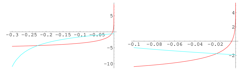
Figure 1: The intersection showing the roots of $Det$ inside the region $x\in(-1/3,0)$. The (red) convex ascending curve in both cases is that of $2f(x)$. In the graph to the left, we have chosen $b=11.2,B=0.1$ and have shown a typical intersection of $2f(x)$ with the (blue) $-4(\gamma+\log 4)+b-\frac{4\,B\,{\pi}^{2}\,{\sqrt{1-x}}}{{\sqrt{1+3\,x}}}$. There could be $0,1$ or $2$ points of intersection depending on the shift parametre $b$; the case shown is with 2 points of intersection. On the graph to the right, we have chosen $b=2,B=0.1$ and the (blue) curve is now $-4(\gamma+\log 4)+b+\frac{4\,B\,{\pi}^{2}\,{\sqrt{1-x}}}{{\sqrt{1+3\,x}}}$. There is always 1 point of intersection.

5.1.1 Comparison Between the $B=0$ and $B\neq 0$ Cases

Now let us compare the roots found here with the ones found in [7] for the case $B=0$. There the determinant is reduced to the diagonal form $\left|\begin{array}[]{ll}1-d_{ee}A_{ee}&0\\ 0&1-d_{oo}A_{oo}\end{array}\right|$. It has a root at $\lambda=-1/3$ where $1-d_{ee}A_{ee}=0$ but $1-d_{oo}A_{oo}\neq 0$. Furthermore, there is a critical value $b_{0}=8\log 2$, above which we have doubly degenerate roots where both $1-d_{ee}A_{ee}=0$ and $1-d_{oo}A_{oo}=0$.

In our general $B\neq 0$ case here. Firstly we have a root in the case 2 above no matter what $b$ is. This root obviously corresponds to $\lambda=-1/3$ at $B=0$. Secondly, there is a critical value $b_{0}(B)$, above which we have two roots. These two roots obviously correspond to the doubly degenerate roots when $B=0$. Therefore, we observe that when $B\neq 0$ the doubly degenerate roots are split (Zeeman effect). This will be a general picture which we will meet again when we discuss the root in the region $(0,1)$.

5.2 Zeros of $Det$ between 0 and 1

We recall the form of $Det$ from (5). Here as in the previous subsection we reduce the problem of finding its zeros to the intersection of a transcendental function with an algebraic one:

$$2h(x)=b\mp\frac{4\,B\,{\pi}^{2}\,{\sqrt{1-x}}}{{\sqrt{1+3\,x}}}-4\,\left(\gamma+\log(4)\right)$$ (94)

We see immediately that for $x\notin[0,1]$, the function $h(x)$ is real while the RHS is complex (with non-vanishing imaginary part) whence there are no solutions there. We therefore focus on the solutions between 0 and 1 where both sides become real. Again we must analyse the minus and the plus cases.

Case 1: $2h(x)=b-\frac{4\,B\,{\pi}^{2}\,{\sqrt{1-x}}}{{\sqrt{1+3\,x}}}-4\,\left(\gamma+\log(4)\right)$

In the region $(0,1]$, the LHS is a monotonically decreasing function while the RHS, a monotonically increasing one. At the endpoint $x=1$, the RHS equals $b-4(\gamma+\log 4)$ and the LHS is $-4(\gamma+\log 4)$. Therefore at the lower limit of $b=0$ there is a solution at $x=1$. For any other value of positive $b$, the RHS gets shifted upwards and there will always be a solution. The situation is illustrated in the left part of Figure 2.

Case 2: $2h(x)=b+\frac{4\,B\,{\pi}^{2}\,{\sqrt{1-x}}}{{\sqrt{1+3\,x}}}-4\,\left(\gamma+\log(4)\right)$

Now in the interesting region both functions are monotonically decreasing, but the LHS, from $\infty$ and the RHS, from a finite value. Once again if $b=0$ there is an intersection at $x=1$, but now there is another point of intersection in $(0,1)$. For positive $b$ however, the $x=1$ endpoints no longer meet but the intersection at another point in between still exists.

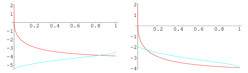
Figure 2: The intersection showing the roots of $Det$ inside the region $x\in(0,1]$. The (red) convex descending curve in both cases is that of $2h(x)$. In the graph to the left, we have chosen $b=1,B=0.1$ and have shown a typical intersection of $2f(x)$ with the (blue) $b-\frac{4\,B\,{\pi}^{2}\,{\sqrt{1-x}}}{{\sqrt{1+3\,x}}}-4\,\left(\gamma+\log(4)\right)$. There is always 1 point of intersection. On the graph to the right, we have chosen the limiting case $b=0,B=0.1$ and the (red) curve is now $b+\frac{4\,B\,{\pi}^{2}\,{\sqrt{1-x}}}{{\sqrt{1+3\,x}}}-4\,\left(\gamma+\log(4)\right)$. There is always 1 point of intersection in between and here there is another at the endpoint $x=1$. For any other value of $b$, $x=1$ would no longer be an intersection point.

Let us compare to the case of $B=0$ in [7] again. There, we had doubly degenerate roots in $(0,1)$. Here for general $B\neq 0$, we have two roots which are not degenerate. It is obvious that these two roots here correspond to the two doubly degenerate roots at $B=0$ and $B\neq 0$ lifts the degeneracy and splits the roots (Zeeman effect). The bigger the value of $B$ the further they split.

6 The Discrete Spectrum

Having addressed the case of the continuous spectrum corresponding to $Det\neq 0$ in the preceding section, here we focus on the case when $\lambda$ makes $Det$ zero. This will give us a Discrete Spectrum.

6.1 The Region ${1\over\xi}(0,1)$

As we have seen before in this region, there are two values $\lambda=\lambda_{1,2}$ making $Det=0$. For both these values, $d_{oe}A_{ee}$ and $d_{oe}A_{oo}$ are nonzero because they are zero only when $B=0$ or $\lambda={1\over\xi}$. Furthermore, since $\lambda\in{1\over\xi}(0,1)$, $\lambda-{M(k)\over\xi}$ can not have a zero to cancel the ones from $r_{1}(k)$ and $r_{2}(k)$ in (22) and we get

$$B_{e}^{(1)}=B_{o}^{(1)}=B_{e}^{(2)}=B_{o}^{(2)}=0.$$

This must indeed be so for (23) to have solutions for $Det=0$.

Now we can solve the ${\cal C}$’s, which must be in the nullspace of the $4\times 4$ matrix in (23); we find two independent vectors:

$$\left(\begin{array}[]{l}{\cal C}^{(1)}_{e}\\ {\cal C}^{(1)}_{o}\\ {\cal C}^{(2)}_{e}\\ {\cal C}^{(2)}_{o}\end{array}\right)=D_{1}\left(\begin{array}[]{l}d_{oe}A_{ee}\\ 0\\ 0\\ 1-d_{ee}A_{ee}\end{array}\right)+D_{2}\left(\begin{array}[]{l}0\\ 1-d_{ee}A_{ee}\\ -d_{oe}A_{ee}\\ 0\end{array}\right)$$

Substituting this back into (21) and (19) as was done before, we have:

$$v=D_{1}\left(\begin{array}[]{l}-{2\sqrt{6b}\Omega\Xi\xi\over 3(\lambda\xi-1+\Omega b)}\\ {d_{oe}\over\lambda-{M\over\xi}}\left|v_{e}\right\rangle\\ 0\\ {d_{oo}-A_{ee}(d_{oo}d_{ee}+d_{oe}^{2})\over\lambda-{M\over\xi}}\left|v_{o}\right\rangle\end{array}\right)+D_{2}\left(\begin{array}[]{l}0\\ {d_{oo}-A_{ee}(d_{oo}d_{ee}+d_{oe}^{2})\over\lambda-{M\over\xi}}\left|v_{o}\right\rangle\\ {2\sqrt{6b}\Omega\Xi\xi\over 3(\lambda\xi-1+\Omega b)}\\ -{d_{oe}\over\lambda-{M\over\xi}}\left|v_{e}\right\rangle\end{array}\right)$$ (95)

where $\lambda=\lambda_{1,2}$, the two solutions of $Det$ in ${1\over\xi}(0,1)$ given in the previous section.

6.2 The Region ${1\over\xi}[-1/3,0)$

When $\lambda\in{1\over\xi}[-1/3,0)$ makes $Det$ zero, things become a little more complex since in this case, we can choose the parameters $k_{1},k_{2},r_{1}(k),r_{2}(k)$ properly to have nonzero $B_{e,o}^{(1,2)}$. This opens a door to new solutions. Let us discuss it in more detail. First, we choose the parameters such that $B_{e,o}^{(1,2)}=0$. In this case, we have two solutions given by the same form as (95).

We need two more solutions and they can be found by choosing nonzero values of $B_{e,o}^{(1,2)}\neq 0$. Let us discuss this case in more detail. To find these two more solutions we need to generalize our method a little bit. The idea is that when we had $\int dkf(k)\left|k\right\rangle=0$ before, in general we should require

$$f(k)=\sum_{k_{i}}\delta(k-k_{i})r_{i}(k),~{}~{}~{}~{}~{}r_{i}(k_{i})=0.$$

Since the equation is linear, if we find a single solution, we can get the general one by linear combination. This method works well for the analysis in the previous sections. However, in the case at hand, such a simplification does not work. Let us explain a little bit. Assume there is a solution for $k_{1}=k_{2}=k_{0}$, $r_{1}(k)=D_{1}(k-k_{0})$ and $r_{2}(k)=D_{2}(k-k_{0})$ with $\lambda=M(k_{0})/\xi$. Consistency requires that

$${d_{oe}A_{ee}\over 1-d_{oo}A_{oo}}=-{B_{e,k_{0}}D_{1}\over B_{o,k_{0}}D_{2}}={B_{e,k_{0}}D_{2}\over B_{o,k_{0}}D_{1}},~{}~{}~{}~{}\Rightarrow~{}~{}~{}D_{1}^{2}=-D_{2}^{2}$$

which have solutions only when $D_{1}=\pm iD_{2}$ and are perfectly consistent since $d_{oe}$ is a purely imaginary number. Now the crucial thing is to check if

$${d_{oe}A_{ee}\over 1-d_{oo}A_{oo}}=-i{B_{e,k_{0}}\over B_{0,k_{0}}}~{}~{}~{}~{}\mbox{or}~{}~{}~{}{d_{oe}A_{ee}\over 1-d_{oo}A_{oo}}=i{B_{e,k_{0}}\over B_{0,k_{0}}}$$

for the given $\lambda$ which makes $Det=0$. We do not have an analytic proof to show this is not true, but it is easy to check numerically and was found that it indeed does not hold. In other words, if we keep only a single term we do not have any solution.

In our case, the generalization is obvious: we just replace $\delta(k-k_{1})r_{1}(k)$ by $\delta(k-k_{1})r_{1}(k)+\delta(k+k_{1})\tilde{r}_{1}(k)$. This then modifies (23) to

$$\left(\begin{array}[]{cccc}1-d_{ee}A_{ee}{}{}&0&0&-d_{oe}A_{ee}\\ 0&1-d_{oo}A_{oo}{}{}&-d_{oe}A_{oo}&0\\ 0&d_{oe}A_{ee}&1-d_{ee}A_{ee}{}{}&0\\ d_{oe}A_{oo}&0&0&1-d_{oo}A_{oo}\end{array}\right)\left(\begin{array}[]{l}{\cal C}^{(1)}_{e}\\ {\cal C}^{(1)}_{o}\\ {\cal C}^{(2)}_{e}\\ {\cal C}^{(2)}_{o}\end{array}\right)=\left(\begin{array}[]{l}B_{e,k_{0}}D_{1}+B_{e,-k_{0}}\widetilde{D}_{1}\\ B_{o,k_{0}}D_{1}+B_{o,-k_{0}}\widetilde{D}_{1}\\ B_{e,k_{0}}D_{2}+B_{e,-k_{0}}\widetilde{D}_{2}\\ B_{o,k_{0}}D_{2}+B_{o,-k_{0}}\widetilde{D}_{2}\end{array}\right).$$ (96)

Now consistency requires

$${d_{oe}A_{ee}\over 1-d_{oo}A_{oo}}=-{B_{e,k_{0}}D_{1}+B_{e,-k_{0}}\widetilde{D}_{1}\over B_{o,k_{0}}D_{2}+B_{o,-k_{0}}\widetilde{D}_{2}}={B_{e,k_{0}}D_{2}+B_{e,-k_{0}}\widetilde{D}_{2}\over B_{o,k_{0}}D_{1}+B_{o,-k_{0}}\widetilde{D}_{1}}.$$

Using $B_{e,k_{0}}=B_{e,-k_{0}}$ and $B_{o,k_{0}}=B_{o,-k_{0}}$ we can solve

$$D_{2}={1\over 2}[(\rho-{1\over\rho})D_{1}-(\rho+{1\over\rho})\widetilde{D}_{1}],~{}~{}~{}~{}~{}\widetilde{D}_{2}={1\over 2}[(\rho-{1\over\rho})D_{1}-(\rho-{1\over\rho})\widetilde{D}_{1}],$$

where we have defined $\rho={d_{oe}A_{ee}\over 1-d_{oo}A_{oo}}{B_{o,k_{0}}\over B_{e,k_{0}}}$. Notice that we have two independent parameters $D_{1},\widetilde{D}_{1}$ which give us the missing two eigenstates. However, the most convenient way is to choose

$$D_{i;+}=D_{i}+\widetilde{D}_{i},~{}~{}~{}~{}~{}D_{i;-}=D_{i}-\widetilde{D}_{i}.$$

Then (96) becomes

$$\left(\begin{array}[]{cccc}1-d_{ee}A_{ee}{}{}&0&0&-d_{oe}A_{ee}\\ 0&1-d_{oo}A_{oo}{}{}&-d_{oe}A_{oo}&0\\ 0&d_{oe}A_{ee}&1-d_{ee}A_{ee}{}{}&0\\ d_{oe}A_{oo}&0&0&1-d_{oo}A_{oo}\end{array}\right)\left(\begin{array}[]{l}{\cal C}^{(1)}_{e}\\ {\cal C}^{(1)}_{o}\\ {\cal C}^{(2)}_{e}\\ {\cal C}^{(2)}_{o}\end{array}\right)=\left(\begin{array}[]{l}D_{1,+}B_{e,k_{0}}\\ D_{1,-}B_{o,k_{0}}\\ \rho D_{1,-}B_{e,k_{0}}\\ -{1\over\rho}D_{1,+}B_{o,k_{0}}\end{array}\right),$$

from which we have two solutions

$$\left(\begin{array}[]{l}{\cal C}^{(1)}_{e}\\ {\cal C}^{(1)}_{o}\\ {\cal C}^{(2)}_{e}\\ {\cal C}^{(2)}_{o}\end{array}\right)=\left(\begin{array}[]{l}0\\ 0\\ 0\\ -{D_{1,+}B_{e,k_{0}}\over d_{oe}A_{ee}}\end{array}\right),~{}~{}~{}~{}~{}~{}\left(\begin{array}[]{l}{\cal C}^{(1)}_{e}\\ {\cal C}^{(1)}_{o}\\ {\cal C}^{(2)}_{e}\\ {\cal C}^{(2)}_{o}\end{array}\right)=\left(\begin{array}[]{l}0\\ {\rho D_{1,-}B_{e,k_{0}}\over d_{oe}A_{ee}}\\ 0\\ 0\end{array}\right).$$ (97)

Our final eigenvectors then become

$$v_{+}=\left(\begin{array}[]{l}-{\sqrt{2b}\xi\over 2(\lambda\xi-1)}{B_{e,k_{0}}D_{1,+}\over A_{ee}}\\ \\ -{B_{e,k_{0}}D_{1,+}\over A_{ee}(\lambda-{M\over\xi})}\left|v_{e}\right\rangle-{\xi D_{1,+}\over 2\frac{dM}{dk}|_{k_{0}}}(\left|k_{0}\right\rangle-\left|-k_{0}\right\rangle)\\ \\ 0\\ \\ -{d_{oo}B_{e,k_{0}}D_{1,+}\over d_{oe}A_{ee}(\lambda-{M\over\xi})}\left|v_{o}\right\rangle+{\xi{1\over\rho}D_{1,+}\over 2\frac{dM}{dk}|_{k_{0}}}(\left|k_{0}\right\rangle+\left|-k_{0}\right\rangle)\end{array}\right)$$ (98)

and

$$v_{-}=\left(\begin{array}[]{l}0\\ \\ {\rho d_{oo}B_{e,k_{0}}D_{1,-}\over d_{oe}A_{ee}(\lambda-{M\over\xi})}\left|v_{o}\right\rangle-{\xi D_{1,-}\over 2\frac{dM}{dk}|_{k_{0}}}(\left|k_{0}\right\rangle+\left|-k_{0}\right\rangle)\\ \\ {-\rho\sqrt{2b}\xi\over 2(\lambda\xi-1)}{B_{e,k_{0}}D_{1,-}\over A_{ee}}\\ \\ {-\rho B_{e,k_{0}}D_{1,-}\over A_{ee}(\lambda-{M\over\xi})}\left|v_{e}\right\rangle-{\xi\rho D_{1,-}\over 2\frac{dM}{dk}|_{k_{0}}}(\left|k_{0}\right\rangle-\left|-k_{0}\right\rangle)\end{array}\right)\,.$$ (99)

7 Level truncation analysis

Here we want to compare some of our predictions with the results of level truncation. First, we do observe a continuous spectrum in the range $\xi^{-1}[-{1\over 3},0)$. Next, we want to check our analytical expressions for the eigenvalues in the interval $(0,\xi^{-1})$. For this, we show in the following table these rescaled eigenvalues $\xi\lambda_{1}$ and $\xi\lambda_{2}$ (defined such that $\lambda_{1}\leq\lambda_{2}$), for $b=1$ and for various values of $B$, to levels 5, 20 and 100. We compare these results to the exact values calculated from (94), shown in the last column.

	Level 5	Level 20	Level 100	Exact value
$\xi\lambda_{1}(B=0.001)$	0.394832	0.397808	0.397969	0.397976
$\xi\lambda_{2}(B=0.001)$	0.408028	0.410125	0.410283	0.41029
$\xi\lambda_{1}(B=0.01)$	0.340706	0.343376	0.343537	0.343544
$\xi\lambda_{2}(B=0.01)$	0.463391	0.465736	0.465892	0.465899
$\xi\lambda_{1}(B=0.1)$	0.0353826	0.036406	0.0364938	0.0364979
$\xi\lambda_{2}(B=0.1)$	0.83877	0.839611	0.839684	0.839688
$\xi\lambda_{1}(B=0.5)$	$-0.000444917$	$-3.03731\cdot 10^{-15}$	$7.39318\cdot 10^{-18}$	$4.08988\cdot 10^{-69}$
$\xi\lambda_{2}(B=0.5)$	0.989926	0.98998	0.989986	0.989986

We see a remarkable agreement between the level truncation and our analytical values. As was already observed in [7], level truncation converges very fast for the isolated eigenvalues.

This also illustrates our discussion in section 5.2 on how turning on a $B$-field breaks the degeneracy between $\lambda_{1}$ and $\lambda_{2}$. Indeed we see that $\xi\lambda_{2}$ goes to one as $B$ is increased, whereas $\xi\lambda_{1}$ goes to zero. This last convergence being very fast, as can be measured from the asymptotic expansions of our analytical expressions [7].

Next we want to check our formulas (61) and (78) for the eigenvectors in the continuous spectrum $v^{e}_{1,\lambda}$, $v^{o}_{1,\lambda}$, $v^{o}_{2,\lambda}$ and $v^{e}_{2,\lambda}$. Here some care is needed: Due to the block-matrix form (18) of $({\cal M})^{11}$, its eigenvalues in the level truncation will always be twice exactly degenerate; indeed if (in block notation) $\left(\begin{array}[]{c}a\\ b\end{array}\right)$ is an eigenvector, then so is $\left(\begin{array}[]{c}b\\ -a\end{array}\right)$. This degeneracy is undesirable because the numerical algorithm which finds the level-truncated eigenvectors will, for each eigenvalue, give two eigenvectors which will be in a mixed state. In other words, for some eigenvalue $\lambda$, the algorithm will output two vectors $w_{1}=a_{1}v^{e}_{1,\lambda}+a_{2}v^{o}_{1,\lambda}+a_{3}v^{o}_{2,\lambda}+a_{4}v^{e}_{2,\lambda}$ and $w_{2}=b_{1}v^{e}_{1,\lambda}+b_{2}v^{o}_{1,\lambda}+b_{3}v^{o}_{2,\lambda}+b_{4}v^{e}_{2,\lambda}$, and we will have no control on the parameters $a_{i}$ and $b_{i}$. We can remedy to this by artificially breaking this degeneracy in the following way: We consider $({\cal M})^{11}_{\epsilon}\equiv({\cal M})^{11}+\epsilon J$, where $J\equiv\left(\begin{array}[]{cc}1&0\\ 0&-1\end{array}\right)$, and $\epsilon$ is a small number (we will typically choose $\epsilon=10^{-7}$. We observe that adding this small perturbation to $({\cal M})^{11}$ breaks the degeneracy in the level truncation. moreover, $J$ commutes with $\left(\begin{array}[]{cc}C&0\\ 0&-C\end{array}\right)$, we thus expect the level-truncated eigenvectors to be of the form $\left(\begin{array}[]{c}{\rm even}\\ {\rm odd}\end{array}\right)$ which we will call even, or $\left(\begin{array}[]{c}{\rm odd}\\ {\rm even}\end{array}\right)$ which we will call odd. If we further constraint all eigenvectors to be of the form $\left(\begin{array}[]{c}{\rm real}\\ {\rm imaginary}\end{array}\right)$, we expect the even level-truncated eigenvectors $w^{e}_{\lambda}$ to be close to some linear combination $a_{1}v^{e}_{1,\lambda}+a_{2}v^{e}_{2,\lambda}$ with $a_{1}$ and $a_{2}$ being real parameters. Similarly, we expect the odd level-truncated eigenvectors $w^{o}_{\lambda}$ to be close to some linear combination $a_{1}v^{o}_{1,\lambda}+a_{2}v^{o}_{2,\lambda}$.

In the next tables, we consider 4 eigenvectors of the level-truncated matrix $({\cal M})^{11}_{\epsilon}$ with $b=1$, $B=0.2$, $\epsilon=10^{-7}$ and we work at level $L=100$. We find the parameters $a_{1}$ and $a_{2}$ by minimizing

$${\rm err}(a_{1},a_{2})={\left(\sum_{i=0}^{5}{|(a_{1}v^{e,o}_{1,\lambda}+a_{2}v^{e,o}_{2,\lambda}-w^{e,o}_{\lambda})_{i}|^{2}}+\sum_{i=L+1}^{L+6}{|(a_{1}v^{e,o}_{1,\lambda}+a_{2}v^{e,o}_{2,\lambda}-w^{e,o}_{\lambda})_{i}|^{2}}\right)^{1\over 2}\over\|a_{1}v^{e,o}_{1,\lambda}+a_{2}v^{e,o}_{2,\lambda}\|}\,,$$

where we have chosen, for simplicity, to compare only the 6 first components of the upper block and the 6 first components of the lower block (remember that each block has size $L+1$). Also, all the vectors appearing in the above formula are normalized to unit norm before being plugged in the formula. Here are the results of this fit for two different eigenvalues which appear in the level truncation.

$\lambda=-0.110388$, even vector	Level truncation	Exact value
component 0	0.158253	0.158271
component 2	$-0.314559$	$-0.314559$
component 4	0.206995	0.206947
component $L+2$	$-0.583525\,i$	$-0.583576\,i$
component $L+4$	$0.313203\,i$	$0.313186\,i$
component $L+6$	$-0.228656\,i$	$-0.22858\,i$
$a_{1}$	$-0.0289756$
$a_{2}$	0.884282
err	$0.0107\%$

$\lambda=-0.110388$, odd vector	Level truncation	Exact value
component 1	0.583524	0.583575
component 3	$-0.313202$	$-0.313185$
component 5	0.228656	0.228578
component $L+1$	$-0.158253\,i$	$-0.158271\,i$
component $L+3$	$0.314561\,i$	$0.314561\,i$
component $L+5$	$-0.206996\,i$	$-0.206948\,i$
$a_{1}$	$-0.0289793$
$a_{2}$	0.884282
err	$0.0107\%$

$\lambda=-0.0716535$, even vector	Level truncation	Exact value
component 0	0.0342766	0.0342883
component 2	0.280389	0.280447
component 4	$-0.260653$	$-0.260619$
component $L+2$	$-0.107005\,i$	$-0.107033\,i$
component $L+4$	$0.201759\,i$	$0.201769\,i$
component $L+6$	$-0.185215\,i$	$-0.185146\,i$
$a_{1}$	0.673384
$a_{2}$	$-0.100719$
err	$0.0102\%$

$\lambda=-0.0716536$, odd vector	Level truncation	Exact value
component 1	0.107009	0.107037
component 3	$-0.20176$	$-0.20177$
component 5	0.185216	0.185147
component $L+1$	$-0.0342776\,i$	$-0.0342892\,i$
component $L+3$	$-0.280388\,i$	$-0.280446\,i$
component $L+5$	$0.260652\,i$	$0.260619\,i$
$a_{1}$	$0.673384$
$a_{2}$	$-0.100714$
err	$0.0102\%$

We see that the errors are of the order of $0.01\%$. This is therefore a very good test of the validity of our formulas.

At last, let us do the same kind of test for one discrete eigenvalue in order to check (95). With the same parameters as before, we have the two following discrete eigenvalues: $\lambda_{1}=0.0000900753$ and $\lambda_{2}=0.366192$. In the following two tables, we compare the eigenvectors related to $\lambda_{2}$. Here, half of the degeneracy is already broken by the $B$-field. Adding the perturbation will further break the degeneracy completely, and we don’t need to use a fit.

$\lambda=0.366192$, even vector	Level truncation	Exact value
component 0	0.97589	0.975946
component 2	0.0115766	0.0115736
component 4	$-0.00544373$	$-0.00543968$
component $L+2$	$0.21255\,i$	$0.212556\,i$
component $L+4$	$-0.0404268\,i$	$-0.0404213\,i$
component $L+6$	$0.0186439\,i$	$0.0186363\,i$
err	$0.0026\%$

$\lambda=0.366192$, odd vector	Level truncation	Exact value
component 1	0.212551	0.212556
component 3	$-0.0404268$	$-0.0404213$
component 5	0.0186439	0.0186363
component $L+1$	$0.97589\,i$	$0.975946\,i$
component $L+3$	$0.0115766\,i$	$0.0115737\,i$
component $L+5$	$-0.00544373\,i$	$-0.00543973\,i$
err	$0.0141\%$

Again, there is a remarkable agreement between numerical and analytical results. These calculation also show that level truncation gives very precise results for the eigenvectors; this observation was already made in [1].

8 Conclusions and Discussions

We analytically solved the problem of finding all eigenvalues and eigenvectors of the Neumann matrix ${\cal M}^{11}$ of the bosonic star-product in the matter sector including zero-modes and with a nontrivial $B$-field background. In particular we see, as was already observed in [13], that turning on a $B$-field does not seem to obstruct the possibility of finding exact solutions.

Starting from the spectrum of ${\cal M}^{11}$ with $B=0$, we found that turning on the $B$-field has three effects on the spectrum:

1. It shrinks the whole spectrum by $\xi=1+(2\pi\alpha^{\prime}B)^{2}$.

2. It splits the discrete eigenvalue into two different ones (Zeeman effect), still in the range $(0,{1\over\xi})$.

3. As we are considering two spatial directions, the eigenvalues in $(-{1\over 3\xi},0)$ are now four times degenerate. Surprisingly, when $B\neq 0$, the eigenvalue $-{1\over 3\xi}$ is only doubly degenerate. Also the isolated eigenvalues in the range $(0,{1\over\xi})$ are both doubly degenerate.

In the discussion of $Det$ we also found some discrete values inside the interval $[-{1\over 3\xi},0)$, depending on the parameters $b$ and $B$, for which the expressions of the eigenvectors differ from those of the continuous eigenvectors. However, it is merely an artifact of the basis in which we are expanding our eigenvectors, and if we renormalize the expression by a proper factor it will be continuous in the whole region $[{-1\over 3\xi},0)$. Furthermore, using the same trick as in [1] and [7], it is an obvious task to calculate the spectra of ${\cal M}^{12}$ and ${\cal M}^{21}$ from the spectrum of ${\cal M}^{11}$ since the three of them satisfy the same algebra relations [13].

The physical meaning of the discrete eigenvalues is still mysterious. It seems however that, unlike the continuous ones, the discrete eigenvectors are $\ell^{2}({\bf N})$-normalizable; this hints us that they are particularly interesting. It thus seems very important to try to understand the meaning of these eigenvectors. We can actually get some clue about it by considering the large $B$-field limit [11, 12]. Indeed if we write the expansion of ${\cal M}^{11}$ in powers of ${1\over B}$, using (5) and (18), we find, up to order two:

$$\xi{\cal M}^{11}=\left(\begin{array}[]{ll|ll}1&0&0&0\\ 0&M&0&0\\ \hline\cr 0&0&1&0\\ 0&0&0&M\end{array}\right)+$$ (104)

$$+{1\over B}{i\over\sqrt{3}\pi^{2}}\left(\begin{array}[]{ll|ll}0&0&0&-\sqrt{2b}\langle v_{o}|\\ 0&0&-\sqrt{2b}|v_{o}\rangle&-2(|v_{e}\rangle\langle v_{o}|+|v_{o}\rangle\langle v_{e}|)\\ \hline\cr 0&\sqrt{2b}\langle v_{o}|&0&0\\ \sqrt{2b}|v_{o}\rangle&2(|v_{e}\rangle\langle v_{o}|+|v_{o}\rangle\langle v_{e}|)&0&0\end{array}\right)+$$ (109)

$$+{1\over B^{2}}{-\beta\over 2\pi^{4}}\left(\begin{array}[]{ll|ll}b&\sqrt{2b}\langle v_{e}|&0&0\\ \sqrt{2b}|v_{e}\rangle&2(|v_{e}\rangle\langle v_{e}|-|v_{o}\rangle\langle v_{o}|)&0&0\\ \hline\cr 0&0&b&\sqrt{2b}\langle v_{e}|\\ 0&0&\sqrt{2b}|v_{e}\rangle&2(|v_{e}\rangle\langle v_{e}|-|v_{o}\rangle\langle v_{o}|)\end{array}\right)+{\cal O}\left(\left({1\over B}\right)^{3}\right)\,.$$ (114)

If we look only to order zero, we see immediately that the spectrum of $\xi{\cal M}^{11}$ is two copies of the spectrum of $M$ and another two eigenvectors with the eigenvalue one. The one with unit eigenvalue obviously is one of our discrete eigenvalues (the other one is sent to zero as $B\rightarrow\infty$). On the other hand, we know from [11, 12], that in the large $B$-field limit, the star-algebra factorizes into a zero-momentum star-algebra (represented here by the spectrum of $M$) and one non-commutative algebra (which must therefore be related to the discrete eigenvalue) corresponding to the momentum of the string. Putting it another way, the discrete eigenvalues should be related to the momentum of the string. All these discussions of the limiting case give us a hint on the physical meaning of these discrete eigenvectors we met in [7] and here.

There is another thing we can observe from equation (114). In the limit of large $B$, the mixing of the two spatial directions happens only at the first order. In other words, comparing with the non-commutativity from the star-product in string field theory (both the zero mode and non-zero modes), the non-commutativity from the $B$-field in the spatial directions is small at large $B$ limit. This may be a little of surprising and deserves better understanding.

There are some immediate follow-up works, for example, to calculate the spectrum of the Neumann matrices in the ghost sector in the light of [5]. This will clarify some subtle points, such as the infinite coefficients mentioned therein. Another interesting direction is to discuss the Moyal product corresponding to the case of $B$ fields. From our eigenvectors we see a mixing of even (odd) state in first direction with the odd (even) in the second. This pattern tells us how the noncommutativities from the star-product and from the $B$-field mix up. Understanding this mix-up will help us better comprehend the noncommutativity.

References

• [1] L. Rastelli, A. Sen and B. Zwiebach, “Star algebra spectroscopy,” arXiv:hep-th/0111281.
• [2] K. Okuyama, “Ghost kinetic operator of vacuum string field theory,” JHEP 0201, 027 (2002) [arXiv:hep-th/0201015].
• [3] K. Okuyama, “Ratio of tensions from vacuum string field theory,” arXiv:hep-th/0201136.
• [4] T. Okuda, “The equality of solutions in vacuum string field theory,” arXiv:hep-th/0201149.
• [5] M. R. Douglas, H. Liu, G. Moore and B. Zwiebach, “Open string star as a continuous Moyal product,” arXiv:hep-th/0202087.
• [6] M. Marino and R. Schiappa, “Towards vacuum superstring field theory: The supersliver,” arXiv:hep-th/0112231.
• [7] B. Feng, Y. H. He and N. Moeller, “The spectrum of the Neumann matrix with zero modes,” arXiv:hep-th/0202176.
• [8] D. Belov, Soon-to-appear work and private communications.
• [9] Fumihiko Sugino, “Witten’s Open String Field Theory in Constant B-Field Background”, hep-th/9912254 , JHEP 0003 (2000) 017.
• [10] Teruhiko Kawano, Tomohiko Takahashi, “Open String Field Theory on Noncommutative Space”, hep-th/9912274, Prog.Theor.Phys. 104 (2000) 459
• [11] E. Witten, “Noncommutative tachyons and string field theory,” arXiv:hep-th/0006071.
• [12] Martin Schnabl, “String field theory at large B-field and noncommutative geometry”, hep-th/0010034, JHEP 0011 (2000) 031.
• [13] L.Bonora, D.Mamone, M.Salizzoni, “B field and squeezed states in Vacuum String Field Theory”, hep-th/0201060.
• [14] L. Rastelli, A. Sen and B. Zwiebach, “Classical solutions in string field theory around the tachyon vacuum,” arXiv:hep-th/0102112.
• [15] E. Witten, “Noncommutative Geometry And String Field Theory,” Nucl. Phys. B 268, 253 (1986).
• [16] G. Moore and W. Taylor, “The singular geometry of the sliver,” JHEP 0201, 004 (2002) [arXiv:hep-th/0111069].