DYNAMICS OF BLACK HOLE FORMATION IN AN EXACTLY SOLVABLE MODEL

Abstract

We consider the process of black hole formation in particle collisions in the exactly solvable framework of 2+1 dimensional Anti de Sitter gravity. An effective Hamiltonian describing the near horizon dynamics of a head on collision is given. The Hamiltonian exhibits a universal structure, with a formation of a horizon at a critical distance. Based on it we evaluate the action for the process and discuss the semiclassical amplitude for black hole formation. The derived amplitude is seen to contain no exponential suppression or enhancement. Comments on the CFT description of the process are made.

I Introduction

The process of black hole formation in high energy collisions has been of major theoretical interest [1-4]. Recent scenarios in which the Planck mass might be of the order of a TeV [5-7] have lead to enhanced study of the subject [3-10]. Estimates for producing black holes at LHC were given very recently in [7-10]. Considerations of black hole production in cosmic ray processes [11-13] were also given.

Simple estimates of black hole formation are based on the hoop conjecture which results in a geometric cross section related to the horizon area [15-17]. More exact numerical studies show that black holes indeed form classically at both zero and nonzero impact parameter collisions [18-20]. Nevertheless there have also been discussions on the possible exponential suppression of the black hole formation process [21-24]. One is generally interested in describing the collision process in terms of CFT and the corresponding Hilbert space language. For all the reasons mentioned above, a further analytical study of black hole formation is of certain interest.

The basic quantity of interest is the amplitude for black hole formation in the collision of two energetic particles. At the semiclassical level, the amplitude is given through the exponential of the Minkowski action

$${\cal A}\sim e^{{i\over\hbar}S{cl}}.$$ (1)

Even though various studies of classical collisions (and formation of the black hole horizon) have been given, the actual amplitude has not been fully evaluated. In the present paper, we consider the process in the exactly solvable framework of 2+1 dimensional gravity [30-35]. Using the known classical solution, we present a Hamiltonian description of the collision at the moment when the horizon forms. This allows for an evaluation of the action which provides information on the question of a possible exponential suppression (or enhancement) in the formation process.

The content of the paper is as follows. In Section 2, we review the case of a single particle in black hole background with an emphasis on the near horizon dynamics. In Section 3, we use the known solution of the 2-body problem in AdS space-time and describe the time evolution of a relative coordinate. In Section 4, we evaluate the corresponding Hamiltonian and the action. In Section 5, we make comments on the differences with the case of a particle in black hole background and comparisons with other works.

II Particle in a Black Hole Background

One could think of an approximate procedure of estimating the action by concentrating on the relative coordinate describing the distance between the colliding particles. In head on collisions, at a critical distance $\,r_{H}\,$ determined by the total CM energy, a horizon forms and one could then imagine an analogy with a case of a particle in a black hole background. In the case of a particle in a black hole background of fixed mass, the well known semiclassical analysis of Hartle and Hawking [36] provides an approximation for the amplitude (and the propagator). An aspect of the semiclassical calculation is the appearance of an imaginary term in action.

Let us consider the case of a three dimensional BTZ black hole.

$$dS^{2}|_{BH}=-dt^{2}\left({r^{2}\over l^{2}}-8GM\right)+{dr^{2}\over{r^{2}\over l^{2}}-8GM}+r^{d}\varphi^{2}$$ (2)

(This will be the main example considered in our study.) Concentrating on the radial part

$$ds^{2}=-f(r)dt^{2}+{dr^{2}\over f(r)}$$ (3)

$$f(r)=r^{2}-r_{H}^{2}$$ (4)

the action for a particle of mass $\,m\,$ is

$$S=-m\int\sqrt{f(r)-{\dot{r}^{2}\over f(r)}}dt.$$ (5)

It is sufficient in what follows to consider a case of massless particle whose Hamiltonian is

$$H=f(r)|p|.$$ (6)

The classical value of the action is then given by

$$S_{cl}=-ET+\int_{r_{0}}^{r}\,dr\,p(r,E).$$ (7)

Taking into account the sign ambiguity appropriate for an ingoing/outgoing particle one has

$$S_{cl}=-ET\pm E\int_{r_{0}}^{r}\,{dr\over f(r)}.$$ (8)

As $r\rightarrow r_{H}$,

$$\qquad f(r)\sim 2r_{H}\,\,(r-r_{H})$$ (9)

so the classical action diverges. Near the horizon, the momentum itself diverges:

$$p\propto{E\over r-r_{H}}.$$ (10)

The velocity on the other hand goes to zero as

$$\dot{r}=r^{2}-r_{H}^{2}$$ (11)

The divergence in the $r$-integration can be avoided by deformation of the contour [32-34] which results in imaginary contributions to the action. More precisely

$$\Delta S({\rm in})\!\!\! = \!\!\!-{i\pi E\over 2r_{H}}$$ (12)

$$\Delta S({\rm out})\!\!\! = \!\!\!+{i\pi E\over 2r_{H}}$$ (13)

Evaluating the modulus square of the amplitudes, one has

$$P_{\it emission}=e^{-{E\over T_{H}}}\;P_{\it absorption}$$ (14)

with the associated Hawking temperature. The origin of the the exponential term (and the Hawking effect) is clearly related to the divergence of the classical action (see [36-40] for detailed studies). A more familiar appearance of this effect would be through a full Euclidean continuation.

When we consider the process of black hole formation, we can ask if there is a similarity of the dynamics involved in the collision with that of a particle in a fixed black hole background. In order to understand that aspect we will construct the relative Hamiltonian for head on collision. It will be seen that even though there are strong similarities between the two processes (at the level of equations of motion), some significant differences will occur at the Hamiltonian level and in the process of evaluation of the action itself.

III Two Particle Collision

As we have said, we will consider the dynamics of particle collision in $2+1$ dimensional AdS space-time. AdS₃ is given by the constraint

$$-x_{-1}^{2}-x_{0}^{2}+x_{1}^{2}+x_{2}^{2}=-\ell^{2}$$ (15)

where $-\ell^{2}$ is the negative cosmological constant.

Let us first summarize some properties of particle-like and black hole solutions in this theory. A point particle of mass $\,m\,$ produces a metric

$$dS^{2}=-dt^{2}\left({r^{2}\over l^{2}}+\gamma^{2}\right)+{dr^{2}\over r^{2}/l^{2}+\gamma^{2}}+r^{2}d\varphi^{2}$$ (16)

with

$$\gamma=1-4Gm.$$ (17)

This represents a cone with the angle

$$\alpha=2\pi\gamma$$ (18)

or a defect angle of

$$\Delta\alpha=2\pi(1-\gamma).$$ (19)

We have that,

$$\Delta\alpha=0\,\,{\rm for}\,\,m\!\!\! = \!\!\!0,$$ (20)

$$\Delta\alpha=2\pi\,\,{\rm for}\,\,m\!\!\! = \!\!\!{1\over 4G}.$$ (21)

To obtain the the metric of a BTZ black hole we identify,

$$\gamma^{2}=-8GM.$$ (22)

From this relation, one sees that a black hole can be obtained for imaginary values of $\,\gamma\,$. Indeed, for a complex value of the particle mass such that,

$$\gamma_{BH}=i\sqrt{8GM}$$ (23)

we have the metric of the BTZ black hole. The process of continuing the particle mass to complex values is obviously not a physical one but an identical situation is achieved through collision of two sufficiently energetic particles.

The dynamics of black hole formation through particle collision in anti-de Sitter space has been studied in detail by Matschull. In [31] the time dependence of particle trajectories was given and the formation of a black hole horizon was established. We will use these results to construct the relative Hamiltonian that reproduces the head on dynamics. For addressing the questions raised in the introduction we will only need the dynamics in the vicinity of the horizon and that is what we will concentrate on. By following the geodesic distance between the two particles, we will deduce the relative Hamiltonian for the formation.

Let us write AdS space in terms of cylindrical coordinates $\chi$, $\varphi$, and $t$.

$$x_{-1}\!\!\! = \!\!\!\ell\cosh\chi\cos t$$ (24)

$$x_{0}\!\!\! = \!\!\!\ell\cosh\chi\sin t$$ (25)

$$x_{1}\!\!\! = \!\!\!\ell\sinh\chi\cos\varphi$$ (26)

$$x_{2}\!\!\! = \!\!\!\ell\sinh\chi\sin\varphi$$ (27)

In these coordinates, the metric is

$$ds^{2}=-\cosh^{2}\chi\,dt^{2}+d\chi^{2}+\sinh^{2}\chi\,d\varphi^{2}$$ (28)

so $t$ is a time-like coordinate, $\chi$ is radial coordinate, and $\varphi$ is an angular coordinate. The collision of two massless particles studied in [31] is first considered in the so-called rest frame of the the black hole. One can identify the horizon in this frame already, but the full physical picture of the process is best seen in the so-called BTZ frame [34]. We will make this explicit by performing the transformation of the particle trajectories into BTZ coordinates.

Following [31], the trajectories of two colliding massless particles are given by

$$\begin{array}[]{l}\mbox{{\it Particle 1:}}\hskip 10.84006pt\tanh\chi=\sin t\hskip 10.84006pt\varphi=0\\ \mbox{{\it Particle 2:}}\hskip 10.84006pt\tanh\chi=\sin t\hskip 10.84006pt\varphi=\theta\hskip 10.84006pt\sin\theta=\tanh\mu\end{array}$$ (29)

The energies of the particles are parameterized as

$$E_{1}\!\!\! = \!\!\!\tan\epsilon_{1}=\coth\frac{\mu}{2}\cosh\mu$$ (30)

$$E_{2}\!\!\! = \!\!\!\tan\epsilon_{2}=\coth\frac{\mu}{2}$$ (31)

and $\mu$ will represent the half length of the black hole horizon. The geodesic that connects the two particles is described by

$$\tanh\chi\sin(\epsilon_{2}+\varphi)=-\sin t\sin\epsilon_{2}.$$ (32)

Because the part of the geodesic for which we are concerned runs from $\varphi=0$ to $\varphi=\theta$, it is convenient to parameterize the geodesic in terms of $\varphi$. Thus, the geodesic length will be

$$S(t)=\int_{0}^{\theta}d\varphi\;\sqrt{\left(\frac{d\chi}{d\varphi}\right)^{2}+\sinh^{2}\chi}.$$ (33)

To find $\frac{d\chi}{d\varphi}$ we can differentiate the equation describing the geodesic implicitly with respect to $\varphi$. Substituting this into the integral, we find the following geodesic distance:

$$S(t)=-2\;\mathop{\mathrm{arctanh}}\nolimits\left(\frac{\sin t}{\sqrt{1+\cos^{2}t\coth\mu/2}}\right)$$ (34)

Time runs from $t=-\pi/2$ to $t=0$ and we can see from Figure 1 that as $t$ goes to $0$, $S(t)$ smoothly approaches $0$.

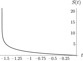
FIG. 1.: Graph of $S(t)$ for $\coth\mu/2=2$.

We will now perform the change to the BTZ coordinate. It is in that coordinate system that the formation of the horizon can be explicitly seen. We follow [34] and denote the metric (which is the same as the usual BTZ metric) as

$$ds^{2}=-\left(\frac{\tilde{r}^{2}}{\ell^{2}}-8GM\right)d\tilde{t}^{\,2}+\frac{d\tilde{r}^{2}}{\frac{\tilde{r}^{2}}{\ell^{2}}-8GM}+\tilde{r}^{2}d\tilde{\phi}^{2}.$$ (35)

with the tilde introduced to avoid confusion with a fixed black hole case. Consider a change from the coordinates $\tilde{r}$, $\tilde{\phi}$, and $\tilde{t}$, to new coordinates $R$, $\Phi$, and $T$ given by

$$R=\frac{\tilde{r}}{\mu},\hskip 21.68121pt\Phi=\mu\tilde{\phi},\hskip 21.68121ptT=\mu\left(\tilde{t}+\frac{\pi}{2}\right).$$ (36)

For the region outside of the horizon $\tilde{r}=\mu$, the range of these coordinates are

$$1<R<\infty,\hskip 21.68121pt-\mu<\Phi<\mu,\hskip 21.68121pt\frac{\mu\pi}{2}<T<\infty.$$ (37)

The metric is now

$$ds^{2}=-(R^{2}-1)dT^{2}+\frac{dR^{2}}{R^{2}-1}+R^{2}d\Phi^{2}.$$ (38)

This exhibits the connection between the BTZ black hole and the AdS space itself. In fact, in terms of the $x_{i}$ variables:

$$x_{-1}\!\!\! = \!\!\!\sqrt{R^{2}-1}\sinh T$$ (39)

$$x_{0}\!\!\! = \!\!\!R\cosh\Phi$$ (40)

$$x_{1}\!\!\! = \!\!\!\sqrt{R^{2}-1}\cosh T$$ (41)

$$x_{2}\!\!\! = \!\!\!R\sinh\Phi$$ (42)

As a consequence, one has a relationship between the cylindrical AdS coordinates with the BTZ coordinates. The trajectories of the particles in the new frame read

$$\begin{array}[]{l}\mbox{{\it Particle 1:}}\hskip 21.68121ptR=\coth T\hskip 21.68121pt\Phi=0\\ \mbox{{\it Particle 2:}}\hskip 21.68121ptR=\coth T\hskip 21.68121pt\Phi=\mu\end{array}$$ (43)

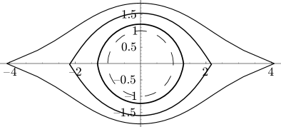
FIG. 2.: Graph of BTZ geodesic for $w=2$, and $T=.25,.50,1.00$.

The geodesic connecting the particles in the BTZ coordinates is given by

$$R^{2}=\frac{w^{2}\cosh^{2}T}{w^{2}\cosh^{2}T-(\sinh\Phi+w\cosh\Phi)^{2}}$$ (44)

where we have introduced the parameter $w=\coth\mu/2$. (This is both the geodesic obtained by solving the geodesic equation and the transformation of the geodesic from AdS space.)

In figure 2, we have plotted the geodesic for various times $T$ using $R$ as a radial coordinate and $\Phi$ as an angular coordinate. The dashed line represents the horizon of the black hole at $R=1$. We can see from this figure that at $T\to\infty$, the particles get closer to the black hole horizon but never enter. Because $\Phi$ runs from $-\mu$ to $\mu$, the length of the horizon is $2\mu$, so $\mu$ has the same meaning in our BTZ coordinates as in AdS space.

We are now ready to derive the geodesic distance in the BTZ metric. In analogy with the AdS case, it is convenient to parameterize the geodesic in terms of the variable $\Phi$. The spacial geodesic distance is given by

$$D(T)=\int_{0}^{\mu}d\Phi\;\sqrt{\frac{1}{R^{2}-1}\left(\frac{dR}{d\Phi}\right)^{2}+R^{2}}.$$ (45)

Again using implicit differentiation to find $\frac{dR}{d\Phi}$, we find the relative distance to be

$$D(T)\!\!\! = \!\!\!\mathop{\mathrm{arctanh}}\nolimits\left(\frac{3+w^{2}+2w^{2}\cosh^{2}T}{(1+w^{2})\cosh T\sqrt{1+w^{2}\sinh^{2}T}}\right)$$ (47)

$$\mbox{ }-\mathop{\mathrm{arctanh}}\nolimits\left(\frac{1}{\cosh T\sqrt{1+w^{2}\sinh^{2}T}}\right).$$

As we can see from Figure 3, $D(T)$ approaches the limiting value of $\mu$ as $T\to\infty$.

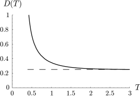
FIG. 3.: Graph of $D(T)$ for $w=8$.

IV The Hamiltonian and the Action

In the above sections, we have constructed an exact solution for the time evolution of our particles in the BTZ coordinates. From this, we will now deduce the Hamiltonian describing the relative dynamics of the particles as they approach the near horizon limit.

The Hamiltonian is to reproduce the equation of motion through

$$\dot{D}=\frac{\partial H}{\partial P_{D}}.$$ (48)

Let us therefore first find the appropriate expression for $\dot{D}$ in the limit of $D\to\mu$ or equivalently $T\to\infty$.

We can expand $D(T)$ in powers of $e^{T}$ about the point $T=\infty$.

$$D(T) = \mathop{\mathrm{arctanh}}\nolimits\left(\frac{2w}{1+w^{2}}\right)+\left(\frac{4(1+6w^{2}+w^{4})}{w(w^{2}-1)^{2}}\right)e^{-2T}$$ (50)

$$+O(e^{-4T}).$$

Recalling that $w=\coth\mu/2$, we have:

$$D(T)\approx\mu+4\cosh 2\mu\tanh\frac{\mu}{2}e^{-2T}$$ (51)

$$\dot{D}(T)\approx-8\cosh 2\mu\tanh\frac{\mu}{2}e^{-2T}$$ (52)

As $T\to\infty$, we have the relation (up to order $e^{-2T}$)

$$\dot{D}=\frac{\mu^{2}-D^{2}}{\mu}.$$ (53)

This result looks much like the case of particle falling into a black hole background as given by eq.(11). As we will now show, the Hamiltonian is very different.

We know that the mass of the (effective) black hole is the total energy of the system. For the BTZ black hole, $\mu=\ell\sqrt{8GM}$ so in units where $8G\ell^{2}=1$, the Hamiltonian $H=\mu^{2}$. It is the fact that in the collision case, the black hole mass is given by the Hamiltonian itself which leads to a difference from the situation in the case of a single particle. Now the horizon radius is a dynamical variable (related to the Hamiltonian). The Hamiltonian is consequently to be self consistently determined.

We can reproduce the above equation taking a Hamiltonian of the form

$$H=D^{2}\tanh^{2}\frac{P}{2D}.$$ (54)

In the limit $D^{2}\to\mu^{2}=H$, this Hamiltonian will give the desired relation for $\dot{D}$. Indeed

$$\dot{D}=\frac{\partial H}{\partial P}=\frac{\sqrt{H}}{D^{2}}(H-D^{2})\approx\frac{H-D^{2}}{\sqrt{H}}$$ (55)

The relative Hamiltonian clearly exhibits the formation of the horizon. Consider the Hamiltonian for large momenta $\,P\,$, when it takes the form:

$$H-D^{2}=-4D^{2}\,e^{-{P\over D}}$$ (56)

We see that for distances $\,D\sim H^{1/2}$, one has a typical behavior associated with an horizon of a black hole. We comment that eq.(48) can also be taken as giving the Hamiltonian (one should remember that we are working in the near horizon limit). Let us study the growth of momenta near the horizon. Even though the equation of motion for the velocity

$$\dot{D}\propto D^{2}-H$$ (57)

appears to be the same as in the particle case, the behavior of the momentum is very different. We have

$$P\approx-D\ln\,{D^{2}-H\over 4D^{2}}$$ (58)

Compared with the particle case, where the momentum was diverging linearly (eq. 10), we now have a milder logarithmic divergence.

Now we can evaluate the action for the classical process of black hole formation. Apart from the energy term responsible for energy conservation, we have

$$\bar{S}=\int^{\mu}PdD.$$ (59)

We evaluate this quantity for our effective Hamiltonian. We have

$$P=-2D\mathop{\mathrm{arctanh}}\nolimits\frac{\mu}{D}$$ (60)

The following change of variables will be helpful for evaluating the integral:

$$z=\frac{\mu}{D}\hskip 21.68121ptdz=-dD\frac{\mu}{D^{2}}\hskip 21.68121ptdD=-dz\frac{\mu}{z^{2}}$$ (61)

We find

$$\int^{\mu}PdD\!\!\! = \!\!\!2\mu^{2}\int^{1}\frac{dz}{z^{3}}\mathop{\mathrm{arctanh}}\nolimits z$$ (62)

$$= \!\!\!\left.2\mu^{2}\left(\frac{1}{2}\left(1-\frac{1}{z^{2}}\right)\mathop{\mathrm{arctanh}}\nolimits z-\frac{1}{2z}\right)\right|^{1}$$ (64)

$$=-\mu^{2}$$

and thus no divergence from near the horizon. So we have the result that the action for the classical process is finite and it does not have imaginary contribution. As a consequence, the amplitude is a pure phase.

$${\cal A}\propto\,e^{{i\over\hbar}S_{ce}}=e^{{i\over\hbar}\Delta}$$ (65)

This implies that of the semiclassical level, there is no exponential suppression (or enhancement) of this process.

V Comments

In the main body of this paper we have described the near horizon dynamics of the two body problem in AdS gravity in terms of an effective Hamiltonian. Even though the Hamiltonian is derived in the particular framework of $2+1$ dimensional Anti de Sitter gravity we believe that it contains some universal features which will be there in any dimensions. We have seen that this effective Hamiltonian predicts a particular logarithmic growth of the relative momentum in the near horizon limit. As we have emphasized this represents a difference from the case of a particle in a fixed mass black hole background. The effective Hamiltonian that we are lead to differs from some other approaches, for example [23].

As a consequence of a softer, logarithmic growth of the near horizon momentum there appears no divergence when integrating to the action. The action for the proces is seen to be finite implying a pure phase contribution to the semiclassical amplitude. Consequently we do not find in this analysis a possibility for an imaginary contribution or exponential suppression of the kind advocated in [21,24].

Concerning the form of the effective Hamiltonian, we would like to comment on one other relevant issue. Its form exhibits a higher nonlinearity in the momentum (and relative coordinate). In that sense we have a similarity with studies of Unruh [41] and Corley and Jacobson [42] where modifications to the energy momentum dispersion were considered. It was shown that that nonlinearities introduced do not modify the Hawking effect at least at low energies. In our case, we have seen that the nonlinearities of the effective Hamiltonian do modify the near horizon growth of the momentum. One should remember that in the case of a black hole formation, one deals with high energies and consequently there is no obvious discrepancy with the findings of [42].

Our final comment concerns the very interesting problem of formulating the process of black hole formation in a conformal field theory (CFT) framework. This question is of major interest and the main trust of the AdS/CFT correspondence (see [33,34] for example and the corresponding references). The relative Hamiltonian that we have presented can be of direct relevance for understanding this issue. In particular it should be possible to obtained this Hamiltonian from CFT. A way in which we can see this happening is by extracting the corresponding “collective” degrees of freedom [43] from the analogue CFT. Results along this line will be given in [44].

Acknowledgements

We would like to acknowledge helpful discussions with Robert De Mello Koch, Joao Rodrigues, Lenny Susskind and David Lowe. We would in particular like to thank Sumit Das for his help and Steven Corley for clarifications concerning the role of high frequency modes. A. J. would like to thank Prof. J. Rodrigues for his hospitality at the University of Witwatersrand and Prof. Hendrik Geyer for his hospitality at the Stellenbosch Institute for Advanced Study, South Africa, where part of this work was done.

This work is supported in part by Department of Energy Grant # DE-FG02-91ER40688 - Task A.

REFERENCES

- [1] G. t’Hooft, Phys. Lett. B 198. 61 (1987).
- [2] H. Verlinde and E. Verlinde, Nucl. Phys. B 371, 246 (1992).
- [3] T. Banks and W. Fischler, hep-th/9906038.
- [4] R. Emparan, G. Horowitz and R. C. Myers, hep-th/0003118.
- [5] N. Arkani-Hamed, S. Dimopoulos and G. R. Dvali, Phys. Lett. B 429, 263 (1998).
- [6] I. Antoniadis, N. Arkani-Hamed, S. Dimopoulos and G. R. Dvali, Phys. Lett. B 436, 257 (1998).
- [7] L. Randall and R. Sundrum, Phys. Rev. Lett. 83, 3370 (1999).
- [8] S. Dimopoulos and G. Landsberg, Phys. Rev. Lett. 87, 161602 (2001).
- [9] S. B. Giddings and S. Thomas, hep-ph/0106219.
- [10] S. Dimopoulos and R. Emparan, hep-ph/0108060.
- [11] J. L. Feng and A. D. Shapere, Phys. Rev. Lett. 88, 021303 (2002).
- [12] L. Anchordoqui and H. Goldberg, Phys. Rev. D 65 047502 (2002).
- [13] R. Emparan, M. Masip, and R. Rattazzi, hep-ph/0109287.
-
[14]
A. Ringwald and H. Tu, hep-ph/0111042;
M. Kowalski, A. Ringwald and H. Tu, hep-ph/0201139. - [15] K. S. Thorne, in “J. Klauder, Magic Without Magic,” S. Francisco, 1972.
- [16] K. A. Khan and R. Penrose, Nature 229, 185(1971).
- [17] S. R. Das, G. W. Gibbons and S. D. Mathur, Phys. Rev. Lett. 78, 417 (1997).
- [18] P. D. D’Eath and P. N. Payne, Phys. Rev. D 46, 658 (1992).
- [19] P. D. D’Eath and P. N. Payne, Phys. Rev. D 46, 675 (1992).
- [20] D. M. Eardley and S. B. Giddings, gr- qc/0201034.
- [21] M. B. Voloshin, Phys. Lett. B 518, 137 (2001).
- [22] M. B. Voloshin, hep-ph/0111099.
- [23] S. N. Solodukhin, hep-th/0201248.
- [24] K. Krasnov, hep-th/0202117 .
- [25] S. Deser, R. Jackiw and G. ’t Hooft, Ann. Phys. 152, 220 (1984).
- [26] M. Banados, C. Teitelboim and J. Zanelli, Phys. Rev. Lett. 69, 1849 (1992).
- [27] S. Deser and R. Jackiw, Ann. Phys. 153, 405 (1984); J. R. Gott and M. Alpert,Gen. Relativ. Gravit. 16, 243 (1984); S. Giddings, J. Abbot and K. Kuchar, Gen. Relativ. Gravit. 16 751 (1984).
- [28] S. F. Ross and R. B. Mann, hep-th/9208036.
- [29] M. W. Choptnik, Phys. Rev. Lett 70. 9 (1993).
- [30] S. Deser, J. G. McCarthy and A. Steif, Nucl. Phys. B412, 305 (1994).
- [31] H. J. Matschull, Class. Quant. Grav. 16, 1069 (1999).
- [32] J. Louko and H. J. Matschull, Class. Quant. Grav. 17, 1847 (2000).
- [33] U. H. Danielsson, E. Keseki-Vakkuri and M. Kruczenski, hep-th/9905227.
- [34] V. Balasubramanian and S. F. Ross, hep-th/9906226.
- [35] D. Birmingham and S. Sen, Phys. Rev. Lett. 84 1074 (2000).
- [36] J. B. Hartle and S. W. Hawking, Phys. Rev. D 13, 2752 (1976).
- [37] M. K. Parikh and F. Wilczek, Phys. Rev. Lett. 85, 5042 (2000).
- [38] S. Shankaranaranayan, T. Padmanabhan and K. Srinivasan, gr-qc/0010042.
- [39] E. C. Vagenas, hep-th/0108147.
- [40] V. Cardoso and J. Lemos, gr-yg/0202019.
- [41] W. G. Unruh, gr-qc/9409008.
- [42] S. Corley and T. Jacobson, Phys. Rev. D 54, 1568 (1996).
- [43] J-L. Gervais, A. Jevicki and B. Sakita, Phys. Rept. 23, 281-293 (1976).
- [44] A. Jevicki and J. K. Thaler, to appear.