1 Introduction

Over the last two decades, there has been some interest in and speculation on the existence of a finite upper bound on accelerations in fundamental physics, motivated from results in quantum field theory [3] and string theory [4]. Both of these theories build on special relativity as a kinematical framework, but upon quantization, a finite upper bound on accelerations apparently enters through the back door [10].
There are interesting results on the promise that the inclusion of a maximal acceleration on the classical level already, will positively modify the convergence behaviour of loop diagrams in quantum field theory [2]. These calculations, however, use an ad-hoc introduction of a maximal acceleration and the authors point out that a rigorous check would require a consistent classical framework which their approach is lacking.

In this paper, we present such a maximal acceleration extension of special and general relativity, obtained by ’kinematization’ of dynamical symmetries of the Born-Infeld action, as explained in the next section.

This leads to a non-trivial lift of special and general relativity to the tangent bundle, or equivalently, the cotangent bundle, of spacetime. Born [5], among others, remarked that in contrast to our deep understanding of non-relativistic mechanics in the Hamiltonian formulation on phase space, special and general relativity are formulated on spacetime only, and the structure of the associated phase space is only poorly understood and thus little used. Clearly, this is likewise true for all dynamical theories based on the kinematical framework of special and general relativity, most notably quantum field theory and string theory. In view of the importance of the non-relativistic phase space structure for the transition to quantum theory, Born regards a phase space formulation of general relativity as a necessary step towards a reconciliation of gravity and quantum mechanics on a descriptional level.
Following the observation of Caianiello [14] that the (co-)tangent bundle of spacetime might be an appropriate stage for a maximal acceleration extension of special relativity, several attempts have been made to equip the tangent bundle with a complex structure, both in the case of flat [8] and curved [7] spacetime. These approaches are all inconsistent, as we will show in section 5.7 that a complex structure is incompatible with the metric geometry needed to impose an upper bound on accelerations.

Anticipating this negative result, we develop the theory of pseudo-complex modules and later generalize to pseudo-complex manifolds. This is then demonstrated to provide the appropriate phase space geometry circumventing the above mentioned no-go theorem. We obtain a lift of the Einstein field equations to the tangent bundle, thus enabling us to formulate a theory of gravity with finite upper bound on accelerations due to non-gravitational forces. Spacetime concepts are regarded as derived ones, and indeed the existence of a finite maximal acceleration is seen to give rise to a non-commutative geometry on spacetime, which becomes commutative again in the limit of infinite maximal acceleration.
In dynamical theories featuring a maximal acceleration, second order derivatives seemed an inconvenient but necessary evil [16, 17] in order to dynamically enforce the maximal acceleration. Exploiting pseudo-complexification techniques, however, we achieve to recast Lagrangians with second order derivatives into first order form. Rather than being just a notational trick, the dynamical information on the maximal acceleration is absorbed into the extended kinematics. This is shown in detail in section 7.

Putting the full machinery for generally curved pseudo-complex manifolds to work allows a rigorous discussion of a Kaluza-Klein induced coupling of a submaximally accelerated particle to Born-Infeld theory.

The last chapter presents a thought on the implications of the pseudo-complex phase spacetime structure for the transition to quantum theory. One lesson there is that the pseudo-complex structure embraces the complex structure, rather than being in opposition to it.

2 Dynamics Goes Kinematics

Prior to Einstein’s formulation of special relativity, the (at the time) peculiar role of the speed of light in electrodynamics was regarded a consequence of the particular dynamics given by Maxwell theory,

$$\mathcal{L}_{\textrm{Maxwell}}=-\frac{1}{4}F_{\mu\nu}F^{\mu\nu}.$$ (1)

In modern parlance, one would say that the boost-invariance of (1) was considered to be a dynamical symmetry of this particular theory, not necessarily present in other fundamental theories of nature.
Einstein’s idea, however, was to regard the symmetries of Maxwell theory as kinematical symmetries, i.e. due to the structure of the underlying spacetime, and hence necessarily present in any theory acting on this stage. Convinced of the correctness of special relativity, we think today that all sensible dynamics must be Poincaré covariant.
Born-Infeld electrodynamics [1]

$$\mathcal{L}_{\textrm{BI}}=\det\left(\eta+bF\right)^{\frac{1}{2}},$$ (2)

although indistinguishable from Maxwell theory at large distances, modifies its short range behaviour essentially. In particular, Born-Infeld theory features a maximal electric field strength

$$E_{\textrm{max}}=b^{-1},$$ (3)

controlled by the parameter $b$. Hence, coupling a massive particle of charge $e$ to Born-Infeld theory,

$$\mathcal{L}=\mathcal{L}_{\textrm{BI}}+\mathcal{L}_{\textrm{free particle}}+\mathcal{L}_{int},$$ (4)

where

$$\mathcal{L}_{\textrm{free particle}} = p^{\mu}\dot{x}^{\mu}-\frac{1}{2}\lambda\left(p_{\mu}p^{\mu}-m^{2}\right),$$ (5)

$$\mathcal{L}_{int} = -e\dot{x}^{\mu}A^{\mu},$$ (6)

we see from the equations of motion that such a particle can at most experience an acceleration

$$\mathfrak{a}=\frac{eb^{-1}}{m}.$$ (7)

Clearly, this is a feature solely due to the particular dynamics of the model (4). But one may well ask whether one can redo Einstein’s trick and convert the dynamical feature of a maximal acceleration into a kinematical one. Taking the resulting framework seriously, viable dynamics are then required to be covariant under the induced symmetry group, which will turn out to include the Lorentz group.
In order to make an educated guess of how the kinematization of the Born-Infeld symmetries could be achieved, consider the Born-Infeld Lagrangian

$$\mathcal{L}={\det}^{1/2}\left(\eta_{\mu\nu}+\frac{e}{m\mathfrak{a}}F_{\mu\nu}\right),$$ (8)

where the parameter $b$ is fixed according to relation (7). It is fairly easy to verify that this can be written

$${\det}^{1/4}\left(\eta_{\mu\nu}\right){\det}^{1/4}\left(\eta_{\mu\nu}+\frac{e^{2}}{m^{2}\mathfrak{a}^{2}}F_{\mu\rho}{F_{\nu}}^{\rho}\right)={\det}^{1/4}\left(H_{mn}\right),$$ (9)

where the we defined the matrix

$$H\equiv\left(\begin{array}[]{cc}\frac{e}{m\mathfrak{a}}F_{\mu\nu}&-\eta_{\mu\nu}\\ \eta_{\mu\nu}&-\frac{e}{m\mathfrak{a}}F_{\mu\nu}\end{array}\right),$$ (10)

and used the determinant identity for $n\times n$ matrices $A,B$,

$$\left|\begin{array}[]{cc}A&-B\\ B&-A\end{array}\right|=\left|B\right|\left|B+AB^{-1}A\right|.$$ (11)

Let $x$ be the worldline of a particle of mass $m$ in spacetime, and $u$ its four-velocity. Denoting the corresponding curve in ’velocity phase spacetime’

$$Y^{m}\equiv\left(\mathfrak{a}x^{\mu},u^{\mu}\right),$$ (12)

we recognize that

$$H^{mn}=\frac{i\,m}{\mathfrak{a}}\left[Y^{m},Y^{n}\right]$$ (13)

corresponds to the canonical commutation relations in presence of an electromagnetic field

$$\left[x^{\mu},x^{\nu}\right] = -iem^{-2}\mathfrak{a}^{-2}F^{\mu\nu},$$ (14)

$$\left[x^{\mu},p^{\nu}\right] = -i\eta^{\mu\nu},$$ (15)

$$\left[p^{\mu},p^{\nu}\right] = ieF^{\mu\nu},$$ (16)

with an additional $\mathfrak{a}^{-2}$-suppressed coordinate non-commutativity, also controlled by the electromagnetic field strength tensor. Hence, assuming this highly suppressed non-commutativity, we have the surprising result

$$\mathcal{L}_{\textrm{BI}}={\det}^{1/4}\left(\left[Y^{m},Y^{n}\right]\right),$$ (17)

suggesting an encoding of the dynamical symmetries of Born-Infeld theory in an appropriate geometry of the tangent or cotangent bundle of Minkowski spacetime.

Conventionally, the complex structure of the cotangent bundle is the key to a geometrical understanding of Hamiltonian systems [6], and leads to commutation relations in the transition to bosonic quantum theory. However, in section 5.7, we show that unless the underlying spacetime is flat, a complex structure of the associated phase space is incompatible with a finite upper bound on accelerations. Hence, even the slightest perturbation of Minkowski spacetime renders such approaches [7, 8] inconsistent, and hence we deem them unphysical at all.
Fortunately, there is a way round this negative result in form of equipping phase spacetime with a pseudo-complex structure, which naturally leads to anticommutation relations for the associated quantum theory, as shown in section 8. The key mathematical ingredient is the ring of pseudo-complex numbers, and the module and algebra structures built upon them. The following chapter is devoted to these mathematical developments.

3 Pseudo-Complex Modules

This section introduces the concept of pseudo-complex numbers, explores some properties and then focuses on the somewhat subtle pseudo-complexification of real vectorspaces and Lie algebras.

3.1 Ring of Pseudo-Complex Numbers

The pseudo-complex ring is the set

$$\mathbb{P}\equiv\left\{a+Ib\,|\,a,b\in\mathbb{R}\right\},$$ (18)

equipped with addition and multiplication laws induced by those on $\mathbb{R}$, where $I\notin\mathbb{R}$ is a pseudo-complex structure, i.e. $I^{2}=1$. There is a matrix representation

$$1\equiv\left(\begin{array}[]{cc}1&0\\ 0&1\end{array}\right),\qquad\qquad I\equiv\left(\begin{array}[]{cc}0&1\\ 1&0\end{array}\right),$$ (19)

such that addition and multiplication on $\mathbb{P}$ are given by matrix addition and multiplication. It is easily verified that $\mathbb{P}$ is a commutative unit ring with zero divisors

$$\mathbb{P}^{0}_{\pm}\equiv\left\{\lambda(1\pm I)\,|\,\lambda\in\mathbb{R}\right\}.$$ (20)

$\mathbb{P}^{0}_{+},\mathbb{P}^{0}_{-}\triangleleft\mathbb{P}$ are the only multiplicative ideals in $\mathbb{P}$, thus they are both maximal ideals. Hence the only fields one can construct from $\mathbb{P}$ are

$$\mathbb{P}/\mathbb{P}^{0}_{+} \cong \mathbb{P}^{0}_{-}\cong\mathbb{R},$$

$$\mathbb{P}/\mathbb{P}^{0}_{-} \cong \mathbb{P}^{0}_{+}\cong\mathbb{R},$$ (21)

which are too trivial for our purposes. Hence we have to stick to $\mathbb{P}$ and deal with its ring structure.
For $p=a+Ib\in\mathbb{P}$, define the pseudo-complex conjugate

$$\bar{p}\equiv a-Ib.$$ (22)

The map

$$|\cdot|^{2}:\mathbb{P} \longrightarrow \mathbb{R}$$

$$|p|^{2} \equiv p\bar{p}=a^{2}-b^{2}$$ (23)

is a semi-modulus on the ring $\mathbb{P}$, which now decomposes into three classes

$$\mathbb{P}=\mathbb{P}^{+}\cup\mathbb{P}^{-}\cup\mathbb{P}^{0},$$ (24)

according to the sign of the modulus:

$$\mathbb{P}^{+} \equiv \left\{p\in\mathbb{P}:|p|^{2}>0\right\},$$

$$\mathbb{P}^{-} \equiv \left\{p\in\mathbb{P}:|p|^{2}<0\right\},$$ (25)

$$\mathbb{P}^{0} \equiv \left\{p\in\mathbb{P}:|p|^{2}=0\right\}=\mathbb{P}^{0}_{\pm}.$$

Define the exponential map

$$\exp:\mathbb{P} \longrightarrow \mathbb{P}^{+}$$

$$\exp(p) \equiv \sum_{n=0}^{\infty}\frac{p^{n}}{n!}.$$ (26)

In terms of $p=a+Ib$ this yields

$$\exp(a+Ib)=\exp(a)\left\{\cosh(b)+I\sinh(b)\right\}$$ (27)

and hence $\exp$ converges on all of $\mathbb{P}$ and is one-to-one. As $\mathbb{P}$ is commutative, the functional identity

$$\exp(p)\exp(q)=\exp(p+q)$$ (28)

holds for all pseudo-complex numbers $p,q\in\mathbb{P}$. Note, in particular, that for any $\exp(p)$, there is always a unique multiplicative inverse, namely $\exp(-p)$.
Using the exponential map, we get the ’polar’ representations

$$\mathbb{P}^{+} = \left\{r\exp(I\psi)|r,\psi\in\mathbb{R}\right\},$$

$$\mathbb{P}^{-} = \left\{Ir\exp(I\psi)|r,\psi\in\mathbb{R}\right\},$$ (29)

$$\mathbb{P}^{0}_{\pm} = \left\{\lambda(1\pm I)|\lambda\in\mathbb{R}\right\}.$$

It is easily verified that the symmetry transformations on $\mathbb{P}$ preserving the semi modulus are the $(1+1)$-dimensional Lorentz group:

$$O_{\mathbb{P}}(1)\cong O_{\mathbb{R}}(1,1)$$ (30)

3.2 $\mathbb{P}$-Modules and Lie Algebras

Usually, the Lie algebras occuring in physical applications are real or complex vector spaces. However, the most general algebraic definition [11] of a Lie algebra only demands it be a module over a commutative ring. Hence we can sensibly define the pseudo-complex extension $L_{\mathbb{P}}$ of a real Lie algebra $L$ by

$$L_{\mathbb{P}}\equiv\left\{t+Is|t,s\in L\right\},$$ (31)

which is a free $\mathbb{P}$-module, as $L$ is a vector space. The Lie bracket on $L_{\mathbb{P}}$ is induced by that on $L$. Its multilinearity follows directly from the commutativity of $\mathbb{P}$. Clearly,

$$\dim_{\mathbb{P}}(L_{\mathbb{P}})=\dim_{\mathbb{R}}(L)=\frac{1}{2}\dim_{\mathbb{R}}(L_{\mathbb{P}}).$$

Let $T_{i}$ with $i=1,\dots,\dim_{\mathbb{R}}(L)$ be the generators of the real Lie algebra $L$. Then we have

$$L_{\mathbb{P}}=\left<T_{i}\right>_{\mathbb{P}}=\left<T_{i},IT_{i}\right>_{\mathbb{R}},$$ (32)

and we will switch between these two pictures where appropriate. As $\mathbb{P}$ is commutative, we have

$$\left[\exp(p_{i}T_{i})\right]^{-1}=\exp(-p_{i}T_{i}).$$ (33)

Hence we can obtain the connection component $G^{id}$ of the associated Lie group $G$ by exponentiation of the algebra

$$G^{id}=\exp\left(\mathbb{P}L\right)=\exp\left(\mathbb{R}L_{\mathbb{P}}\right).$$ (34)

Let the real vector space $V$ be a representation of the real Lie group $L$. Then $L_{\mathbb{P}}$ acts naturally on the pseudo-complexification of $V$,

$$V_{\mathbb{P}}\equiv\left\{x+Iu|x,u\in V\right\}$$ (35)

which is a free $\mathbb{P}$-module of dimension $\dim_{\mathbb{R}}V$. $V_{\mathbb{P}}$ also being an $\mathbb{R}$-vectorspace of dimension $2\dim_{\mathbb{R}}$, we can identify $V_{\mathbb{P}}$ with the tangent bundle $TV$ via

$$V_{\mathbb{P}}=\left\{x+Iu|x\in V,u\in T_{x}V\right\}.$$ (36)

The bundle projection is then given in this language by

$$\pi:TV\equiv V_{\mathbb{P}} \longrightarrow V$$

$$\pi(X) \equiv \frac{1}{2}(X+\bar{X})$$ (37)

3.3 The Pseudo-Complex Lorentz Group

Let $\eta\equiv\textrm{diag}\left(1,-1,\dots,-1\right)$ have signature $(1,n-1)$ and consider the pseudo-complex extension $so_{\mathbb{P}}(1,n-1)$ of the real Lorentz algebra $so_{\mathbb{R}}{(1,n-1)}$. Exponentiation gives the pseudo-complex Lorentz group

$$SO_{\mathbb{P}}(1,n-1)\equiv\left\{\Lambda\in\textrm{Mat}\left(n,\mathbb{P}\right)|\Lambda^{T}\eta\Lambda=\eta,det\Lambda=1\right\}$$ (38)

Clearly, for any $U\in T\mathbb{P}^{n}$, the expression

$$\eta\left(U,U\right)\equiv U^{\mu}U^{\nu}\eta_{\mu\nu}$$ (39)

is invariant under the action of $SO_{\mathbb{P}}(1,n-1)$. Expanding (39) using $U^{\mu}=u^{\mu}+Ia^{\mu}$, $u,a\in\mathbb{R}^{r+s}$ yields

$$\eta\left(U,U\right)=\left(u^{\mu}u_{\mu}+a^{\mu}a_{\mu}\right)+I\left(2u^{\mu}a_{\mu}\right).$$ (40)

Let $M^{\mu\nu}$ be the standard generators of the real Lorentz-group, then

$$so_{\mathbb{P}}(1,n-1)=\left<M^{\mu\nu},IM^{\mu\nu}\right>_{\mathbb{R}}$$ (41)

and the pseudo-complex linear combinations

$$G^{\mu\nu}\equiv\frac{1}{2}(M^{\mu\nu}+IM^{\mu\nu}),\quad\bar{G}^{\mu\nu}\equiv\frac{1}{2}(M^{\mu\nu}-IM^{\mu\nu})$$ (42)

generate two decoupled real Lorentz algebras, and hence

$$so_{\mathbb{P}}(1,n-1)\cong so_{\mathbb{R}}(1,n-1)\oplus so_{\mathbb{R}}(1,n-1).$$ (43)

Note that the real and pseudoimaginary part of (40) are preserved separately under the action of $O_{\mathbb{P}}(1,n-1)$. Hence, we can switch between the picture of a metric module and a bimetric vector space:

$$\left(\mathbb{P}^{n},\eta\right)\cong\left(T\mathbb{R}^{n},\eta^{D},\eta^{H}\right),$$ (44)

where $\eta^{D}=\eta\otimes 1$ and $\eta^{H}=\eta\otimes I$ denote the diagonal and horizontal lifts to the tangent bundle [9], respectively, of the Minkowski metric.

3.4 The Pseudo-Complex Sequence

Define inductively, for all $n\in\mathbb{N}$,

$$\mathbb{P}^{(0)} \equiv \mathbb{R},$$ (45)

$$\mathbb{P}^{(n+1)} \equiv \left\{1\otimes a+I\otimes b\,|\,a,b\in\mathbb{P}^{(n)}\right\},$$ (46)

the sequence of pseudo-complex rings. $\mathbb{P}^{(n)}$ is called the pseudo-complex ring of rank $n$. Commutativity is easily shown by induction. Clearly, $\mathbb{P}^{(n)}$ is a vector space of dimension $2^{n}$, with canonical basis

$$1\otimes 1\otimes\dots\otimes 1,1\otimes 1\otimes\dots\otimes I,\dots,I\otimes I\otimes\dots\otimes I.$$

Identifying the $b$-th canonical basis vector $\mathbf{b}$ in $\mathbb{P}^{(n)}$ with a binary number $0\leq b\leq 2^{n}-1$ via $1=0$, $I=\mathsf{l}$, multiplication between basis elements corresponds to the ’exclusive or’ operation $\sqcup$

$$\begin{array}[]{c|cc}\sqcup&0&\mathsf{l}\\ \hline\cr 0&0&\mathsf{l}\\ \mathsf{l}&\mathsf{l}&0\end{array}$$ (47)

Hence the multiplication of two $n$-th rank pseudo-complex numbers

$$p=\sum_{b=0}^{2^{n}-1}p_{b}\,\mathbf{b},\qquad q=\sum_{b=0}^{2^{n}-1}q_{c}\,\mathbf{c}$$

is given by

$$pq = \sum_{b,c}^{2^{n}-1}p_{b}q_{c}\,\mathbf{b}\sqcup\mathbf{c}$$ (48)

$$= \sum_{b,d}^{2^{n}-1}p_{b}q_{b\sqcup d}\,\mathbf{d},$$

observing that $b\sqcup c=d$ if and only if $b\sqcup d=c$. We use the extension of this result to the infinite-dimensional case to define the multiplication law on

$$\mathbb{P}^{(\infty)}\equiv\left\{p:\mathbb{N}\longrightarrow\mathbb{R}\right\},$$ (49)

the set of all real sequences.
From the binary representation, the sets $\mathbb{P}^{(n)}$ and $\mathbb{P}^{(\infty)}$ are seen to be commutative rings with unit $\mathbf{0}$. Hence on can define the $n$-th rank pseudo-complexification of a real Lie algebra $L$

$$L_{\mathbb{P}^{(n)}}\equiv\left\{\sum_{b=0}^{2^{n}-1}t_{b}\mathbf{b}\,|\,t_{b}\in L\right\}$$ (50)

which is a free module of dimension

$$\dim_{\mathbb{P}}^{(n)}(L_{\mathbb{P}^{(n)}})=\dim_{\mathbb{R}}(L)=2^{-n}\dim_{\mathbb{R}}(L_{\mathbb{P}^{(n)}}),$$ (51)

and the $n$-th rank pseudo-complexification of a real vectorspace $V$,

$$V_{\mathbb{P}^{(n)}}\equiv\left\{\sum_{b=0}^{2^{n}-1}x_{b}\mathbf{b}\,|\,x_{b}\in V\right\}$$ (52)

being a free $\mathbb{P}^{(n)}$-module, or a real vectorspace of dimension $2^{n}\dim_{\mathbb{R}}(V)$. We can identify $V_{\mathbb{P}^{(n)}}$ with the $n$-th tangent bundle $T^{n}V$, i.e. the bundle of $n$-jets [9].

4 Maximal Acceleration Extension of Special Relativity

We obtain a maximal acceleration extension of special relativity by pseudo-complexification of Minkowski spacetime

$$\mathbb{R}^{1,3}\longrightarrow\mathbb{P}^{1,3}$$ (53)

and appropriate lifts of all spacetime concepts to the resulting module. Alternatively to pseudo-complexification, all this can be understood in terms of lifts to the tangent bundle of spacetime, at the cost of having to deal with two metrics.
That the geometry obtained in this way indeed encodes the Born-Infeld kinematics, is shown in section 4.5. The theory is formulated entirely independent of spacetime concepts. This involves the slight paradigm shift of thinking of the objects defined on pseudo-complexified spacetime as primary, rather than being induced from the familiar spacetime concepts, which will be regarded as derived ones.

4.1 Mathematical Structure

We introduce a fundamental constant $\mathfrak{a}$ of dimension length^-1, called maximal acceleration. The stage for extended relativistic physics is pseudo-complexified Minkowski spacetime

$$\mathbb{P}^{1,3}\equiv\left(\mathbb{P}^{4},\eta\right),$$

equipped with a pseudo-complex valued two-form

$$\eta:\mathbb{P}^{4}\times\mathbb{P}^{4}\longrightarrow\mathbb{P}$$ (54)

of signature $(1,3)$. Note that without further restriction, $\eta$ is not a real-valued semi-norm on $\mathbb{P}^{1,3}$, as its pseudo-imaginary part is non-vanishing in general.
The symmetry algebra of $\mathbb{P}^{1,3}$ is, by construction, the pseudo-complexified Lorentz algebra

$$o_{\mathbb{P}}(1,3).$$

We introduce a preferred class of coordinate systems, generalizing the inertial frames of special relativity. A basis $\left\{e_{(\mu)}\right\}$ of $T\mathbb{P}^{1,3}$ with

$$\eta\left(e_{(\mu)},e_{(\nu)}\right)=\eta_{\mu\nu}\equiv\textrm{diag}\left(1,-1,-1,-1\right)$$ (55)

is called a uniform basis or uniform frame. Coordinates of $\mathbb{P}^{1,3}$ given with respect to such a basis are called uniform coordinates.
We will always work in uniform coordinates in this chapter. Clearly, under the action of $SO_{\mathbb{P}}(1,3)$, a uniform basis is transformed to a uniform basis.

Let $x:\mathbb{R}\longrightarrow\mathbb{R}^{1,3}$ be a timelike curve in real Minkowski spacetime. Then the natural lift $X\equiv x^{*}$ to pseudo-complexified spacetime

$$x:\mathbb{R} \longrightarrow \mathbb{R}^{1,3}$$

$$\downarrow*$$

$$X:\mathbb{R} \longrightarrow \mathbb{P}^{1,3}$$ (56)

is defined by

$$X\equiv x^{*}\equiv\mathfrak{a}x+Iu$$ (57)

where $u\equiv\frac{dx}{d\tau}$ and $d\tau^{2}\equiv\eta(dx,dx)$. Let $X:\mathbb{R}\longrightarrow\mathbb{P}^{1,3}$ be a curve in configuration space. $X$ is called an orbit iff there exists a uniform frame $\Sigma$ such that

$$X=\pi(X)^{*},$$ (58)

where $*$ denotes the natural lift (57) and $\pi$ the projection (3.2). The frame $\Sigma$ is called an inertial frame.
The line element of the projection $\pi(X)$ of an arbitrary orbit $X$ in a particular uniform (not necessarily inertial) frame is denoted by $d\tau$ and given by

$$d\tau^{2}\equiv\eta\left(d\pi(X),d\pi(X)\right).$$ (59)

Note that this quantity is frame-dependent.
It is clear that for an orbit $X$ given in inertial coordinates $X^{\mu}=x^{\mu}+Iu^{\mu}$, we always have the relation $u=\frac{dx}{d\tau}$. Further it follows that the projection $\pi(X)$ is necessarily timelike in inertial coordinates. Now consider an orbit $X$ in an inertial frame. The orthogonality of $dx$ and $du=d\frac{dx}{d\tau}$ yields

$$\eta\left(dX,dX\right)\in\mathbb{R}$$ (60)

in inertial coordinates, but due to the $SO_{\mathbb{P}}(1,3)$-invariance of (60) this result even holds in any uniform frame. Hence, along an orbit, the generically $\mathbb{P}$-valued two-form $\eta$ provides a real-valued semi inner product, allowing the following classification: An orbit $X$ is called submaximally accelerated, if

$$d\omega^{2}\equiv\left(dX,dX\right)>0$$ (61)

everywhere along the orbit. Note that the line element $d\omega$ is an $O_{\mathbb{P}}(1,3)$ scalar. Observe that an orbit $X$ is submaximally accelerated if and only if the projection $\pi(X)$ has Minkowski curvature $g<\mathfrak{a}$. This is seen as follows. In an inertial frame, let $x\equiv\pi(X)$, $u\equiv\frac{dx}{d\tau}$ and $a\equiv\frac{du}{d\tau}$. Then $X=\mathfrak{a}x+Iu$ and we have from (40)

$$d\omega^{2}=\left(1-\mathfrak{a}^{-2}g^{2}\right)\mathfrak{a}^{2}d\tau^{2}$$ (62)

where $g$ is the Minkowski-scalar acceleration of the trajectory $x$. Hence,

$$d\omega^{2}>0\Leftrightarrow g<\mathfrak{a}$$

as $d\tau^{2}>0$ as $x=\pi(X)$ is timelike everywhere. As $d\omega^{2}$ is $SO_{\mathbb{P}}(1,3)$-invariant, the result holds in any uniform frame.
This gives us the interpretation of the constant $\mathfrak{a}$ as the upper bound for accelerations in this theory, and thus justifies the terminology.

In analogy to the notion of rapidity in special relativity, it is useful to introduce a convenient non-compact measure for accelerations. This will clear up notation later on. Let $X$ be a submaximally accelerated orbit, and $g$ be the Minkowski curvature of the projection $\pi(X)$ for a particular uniform observer. Then the accelerity $\alpha$ of the trajectory is given by

$$\tanh(\alpha)=\frac{g}{\mathfrak{a}}.$$ (63)

Hence the relation between the $O_{\mathbb{P}}(1,3)$-invariant line element $d\omega$ of an orbit and the Minkowski line element $d\tau$ of the projection $\pi(X)$ is

$$d\omega=\frac{\mathfrak{a}}{\cosh(\alpha)}d\tau.$$ (64)

Note that although $d\tau$ and $\alpha$ are frame dependent, the combination on the right hand side above is manifestly frame independent, as $d\omega$ is.
Finally, we define the eight-velocity $U$ of a submaximally accelerated orbit $X$ as

$$U:\mathbb{R} \longrightarrow T\mathbb{P}^{1,3}$$ (65)

$$U \equiv \frac{dX}{d\omega}.$$ (66)

This is well-defined due to the $O_{\mathbb{P}}(1,3)$-invariance of $d\omega$. Sometimes we will consider the real and pseudo-imaginary part of $U$ in uniform coordinates, which we will denote

$$U\equiv\tilde{u}+I\tilde{a}=\cosh(\alpha)\left(u+I\mathfrak{a}^{-1}a\right),$$ (67)

where $u$ and $a$ are the four-velocity and acceleration of the corresponding spacetime trajectory $\pi(X)$.

4.2 Linear Uniform Acceleration in Extended Special Relativity

It is instructive to study orbits which project to trajectories of linear uniform acceleration, i.e. constant accelerity $\alpha$. Let $U$ be the eight-velocity of such an orbit. From $\eta(U,U)=1$ and using (63), (67), we get

$$\tilde{u}^{\mu}\tilde{u}_{\mu} = 1+\sinh^{2}(\alpha),$$ (68)

$$\tilde{u}^{\mu}\tilde{a}_{\mu} = 0.$$ (69)

Choosing a Lorentz frame such that

$$u^{2}=u^{3}=a^{2}=a^{3}=0,$$

(69) becomes

$$\tilde{u}^{0}\tilde{a}^{0}-\tilde{u}^{1}\tilde{a}^{1}=0,$$ (70)

which is solved by

$$\tilde{a}^{0} = \gamma\tilde{u}^{1},$$ (71)

$$\tilde{a}^{1} = \gamma\tilde{u}^{0},$$ (72)

for some function $\gamma$. Constant accelerity gives

$$\tilde{a}^{\mu}\tilde{a}_{\mu}=-\cosh^{2}(\alpha)\frac{g^{2}}{\mathfrak{a}^{2}}=-\sinh^{2}(\alpha).$$

On the other hand,

$$\tilde{a}^{\mu}\tilde{a}_{\mu}=-\gamma^{2}\tilde{u}^{\mu}\tilde{u}_{\mu}=-\gamma^{2}\left(1+\sinh^{2}(\alpha)\right).$$

Hence for linear uniform acceleration of modulus $g$,

$$\tilde{a}^{0} = \frac{g}{\mathfrak{a}}\tilde{u}^{1},$$ (73)

$$\tilde{a}^{1} = \frac{g}{\mathfrak{a}}\tilde{u}^{0},\qquad\textrm{ where }g<\mathfrak{a}.$$ (74)

Now consider the projections

$$\pi_{01}(\tilde{u}^{0},\tilde{u}^{1},\tilde{a}^{0},\tilde{a}^{1}) = (\tilde{u}^{0},\tilde{a}^{1}),$$ (75)

$$\pi_{10}(\tilde{u}^{0},\tilde{u}^{1},\tilde{a}^{0},\tilde{a}^{1}) = (\tilde{u}^{1},\tilde{a}^{0})$$ (76)

from $T\mathbb{P}^{1,3}$ to the $\tilde{u}^{0}-\tilde{a}^{1}$ and $\tilde{u}^{1}-\tilde{a}^{0}$ planes, respectively (see figure 1). From (73) and (74), we see that an orbit corresponding to a spacetime trajectory of constant Minkowski curvature $g$ projects under $\pi_{01}$ and $\pi_{10}$ to straight lines through the origin of slope ${\mathfrak{a}g^{-1}}$ in the ${\tilde{u}^{0}-\tilde{a}^{1}}$ and ${\tilde{u}^{1}-\tilde{a}^{0}}$ planes. Special relativity allows arbitrarily high accelerations, hence there the spectrum of uniformly accelerated spacetime curves is given by all straight lines through the origin in these planes, with the same slope in both planes for one particular curve.
In the framework presented here, however, $g$ is bounded from above by $\mathfrak{a}$.

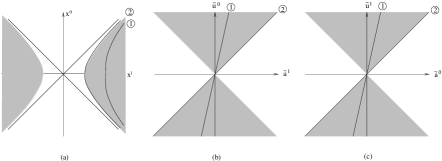
Figure 1: Spectrum of uniformly accelerated curves in ESR

Using the conversion formula (67), we see that in the spacetime projection, (73-74) gives the familiar hyperbolae of Minkowski curvature $g$, but only for $g<\mathfrak{a}$. This determines the spectrum of uniformly accelerated curves in extended special relativity up to Poincare transformations (see figure 1).

4.3 Special Transformations in $SO_{\mathbb{P}}(1,3)$

Exponentiation of the generators $M^{\mu\nu}$ (cf. section 3.3) yields the familiar real Lorentz transformations acting on $T\mathbb{P}^{1,3}$. The group elements generated by the $IM^{\mu\nu}$ are given by the ordinary Lorentz transformations evaluated with purely pseudo-imaginary arguments. For notational simplicity, we exhibit their properties in a $(1+1)$-dimensional theory. The pseudo-boost of accelerity $\beta$ is then given by

$$\Lambda_{\textrm{boost}}(I\beta)=\left(\begin{array}[]{cc}\,\,\cosh(\beta)&I\sinh(\beta)\\ I\sinh(\beta)&\,\,\cosh(\beta)\end{array}\right),$$ (77)

and its action on the eight-velocity $U=\tilde{u}+I\tilde{a}$ is

$$\left(\begin{array}[]{c}\tilde{u}^{0}\\ \tilde{u}^{1}\\ \tilde{a}^{0}\\ \tilde{a}^{1}\end{array}\right)\mapsto\left(\begin{array}[]{c}\cosh(\beta)\,\tilde{u}^{0}+\sinh(\beta)\,\tilde{a}^{1}\\ \cosh(\beta)\,\tilde{u}^{1}+\sinh(\beta)\,\tilde{a}^{0}\\ \cosh(\beta)\,\tilde{a}^{0}+\sinh(\beta)\,\tilde{u}^{1}\\ \cosh(\beta)\,\tilde{a}^{1}+\sinh(\beta)\,\tilde{u}^{0}\end{array}\right).$$ (78)

This hyperbolically rotates a straight line of hyperbolic angle $\beta$ in the $\tilde{u}^{0}-\tilde{a}^{1}$ and $\tilde{u}^{1}-\tilde{a}^{0}$ plane to another straight line of hyperbolic angle $\alpha+\beta$ in the respective plane. One can check that the the two remaining pseudo-boosts do exactly the same with respect to the other space directions. Hence the pseudo-boosts acting on the eight-velocity map the projections (75-76) of a $U$-curve to the projection of another uniformly accelerated curve $U^{\prime}$. We still have to check whether it maps the whole curve U to a uniformly accelerated curve $U^{\prime}$. But this is easily seen by counting degrees of freedom: for a pseudo-boost in 1-direction, the projections of the transformed curve give us the two constraints

$$\tilde{a^{\prime}}^{0} = \tanh(\alpha+\beta)\tilde{u^{\prime}}^{1}$$ (79)

$$\tilde{a^{\prime}}^{1} = \tanh(\alpha+\beta)\tilde{u^{\prime}}^{0}$$ (80)

and we know that

$$\tilde{a^{\prime}}^{2} = a^{2}$$ (81)

$$\tilde{a^{\prime}}^{3} = a^{3}$$ (82)

$$\tilde{u^{\prime}}^{2} = u^{2}$$ (83)

$$\tilde{u^{\prime}}^{3} = u^{3}$$ (84)

Further we know that any submaximally accelerated timelike curve lies in the hypersurface

$$\eta(U,U)=1$$

in $U$-space. Being $O_{\mathbb{P}}(1,3)$-transformations, pseudo-boosts respect this condition, and thus it is still true for the transformed curve $U^{\prime}$. This leaves us with $8-(2+4+1)=1$ degrees of freedom, uniquely determining $U^{\prime}$.
The pseudo-boosts transform the eight-velocity of a submaximally accelerated orbit in one frame to the eight-velocity in a relatively accelerated frame.
As $U=\frac{dX}{d\omega}$ and $d\omega$ is an $SO_{\mathbb{P}}(1,3)$-invariant, the pseudo-Lorentz group acts also linearly on the orbit $X$. The action is non-linear, however, on the spacetime curve $\pi(X)$. Note that the pseudo-Lorentz transformations with not purely real parameter only induce a well-defined action on the space of motions on spacetime, but cannot be understood as a map $M\longrightarrow M$ of spacetime onto itself. This is so because the components projected out by $\pi:TM\longrightarrow M$ mix with the spacetime coordinates under such transformations. Hence spacetime coordinates fail to be well-defined under changes to uniformly accelerated frames. Thus extended relativity anticipates the Unruh [3] effect on a classical level already. This also presents another manifestation of the non-commutative geometry on spacetime induced by a finite upper bound on accelerations, as first tentatively noted in (14).
Pseudo-boosts in an arbitrary space direction can be composed from the pseudo-boosts in the coordinate directions and an appropriate rotation, exactly like for real boosts:

$$\textrm{rotation}^{-1}_{R}\quad\textrm{boost}_{\mathbf{n}}\quad\textrm{rotation}_{R}\quad = \quad\textrm{boost}_{R\mathbf{n}},$$

$$\textrm{rotation}^{-1}_{R}\quad\textrm{p-boost}_{\mathbf{n}}\quad\textrm{rotation}_{R}\quad = \quad\textrm{p-boost}_{R\mathbf{n}}.$$

The role played by the pseudo-rotations is illuminated by the identity

$$\textrm{p-rot}^{-1}_{i}\left(\frac{\pi}{2}\right)\quad\textrm{boost}_{i}\quad\textrm{p-rot}_{i}\left(\frac{\pi}{2}\right)\quad=\quad\textrm{p-boost}_{i}.$$

The pseudo-rotations rotate velocities into accelerations and vice versa, thus showing explicitly that there is no well-defined distinction between velocities and accelerations, like in canonical classical mechanics due to symplectic symmetry. We will see this mechanism at work explicitly when discussing point particle dynamics in chapter 7.

4.4 Physical Postulates of Extended Special Relativity

Equipped with the machinery developed above, we can now concisely formulate the physical postulates of the maximal acceleration extension of special relativity.
Postulate I.
Massive particles are described by submaximally accelerated orbits $X$, i.e.

$$\eta\left(dX,dX\right)>0$$ (85)

everywhere along $X$.
Postulate II. (modified clock postulate, [10])
The physical time measured by a clock with submaximally accelerated orbit $X$ is given by the integral over the line element,

$$\Omega=\mathfrak{a}^{-1}\int d\omega=\mathfrak{a}^{-1}\int\sqrt{\eta\left(\frac{dX}{d\lambda},\frac{dX}{d\lambda}\right)}\,d\lambda.$$ (86)

For curves of uniform accelerity $\alpha$, the modified clock postulate gives a departure from the special relativity prediction by a factor of

$$\cosh^{-1}(\alpha)=\sqrt{1-\frac{g^{2}}{\mathfrak{a}^{2}}}.$$ (87)

Hence experiments testing the clock postulate and involving accelerations $|g|<g_{exp}$ give a lower bound on the hypothetical maximal acceleration $\mathfrak{a}$.
Farley et al. [12] have measured the decay rate of muons with acceleration $g_{\textrm{exp}}=5\times 10^{18}ms^{-2}$ within an accuracy of $2$ percent. This corresponds to a measurement of the lifetime within the same accuracy $\Delta=0.02$. Hence the factor (87) must deviate from unity less than $\Delta$:

$$\sqrt{1-\frac{g^{2}}{\mathfrak{a}^{2}}}>1-\Delta,$$ (88)

thus leading to an experimental lower bound for the maximal acceleration

$$\mathfrak{a}>\frac{g}{\sqrt{\Delta\left(2-\Delta\right)}}\approx 2.5\times 10^{19}ms^{-2}.$$ (89)

From the extended relativistic correction to the Thomas precession, one obtains a much better upper bound $\mathfrak{a}\geq 10^{22}ms^{-2}$, as shown in [19].

Correspondence Principle
From the postulates above, we recognize that in the limit $\mathfrak{a}\rightarrow\infty$, we have $d\omega\rightarrow d\tau$, and $U\rightarrow u$, i.e. extended special relativity becomes special relativity.

4.5 Born-Infeld Theory Revisited

After the formal developments in the last two chapters, we return to the starting point of our investigations, the Born-Infeld action. We demonstrate that the transformation of the commutation relations (13) as a second rank tensor of the pseudo-complex Lorentz group is well-defined, and hence Born-Infeld theory is compatible with the extended specially relativistic kinematics developed earlier in this chapter. This shows that the pseudo-complexification procedure was indeed successful in the kinematization of the Born-Infeld symmetries associated with the maximal acceleration.

In section 2, we assumed a particular coordinate non-commutativity in order to recast the Born-Infeld action in the suggestive form (17). Now we are in a position to prove that this is is the only well-defined non-commutative geometry admitted by $SO_{\mathbb{P}}(1,3)$ symmetry. Assume the commutation relations in the background of an electromagnetic field are more generally given by

$$\left[x^{\mu},x^{\nu}\right] = -ieK^{\mu\nu},$$ (90)

$$\left[x^{\mu},p^{\nu}\right] = -i\eta^{\mu\nu},$$ (91)

$$\left[p^{\mu},p^{\nu}\right] = ieF^{\mu\nu},$$ (92)

with an antisymmetric, otherwise (so far) arbitrary $K^{\mu\nu}$. Using the notation ${X^{m}=\left(\mathfrak{a}x^{\mu},u^{\mu}\right)}$, we define the tensor $\tilde{H}$ through

$$\left[X^{m},X^{n}\right]=-i\frac{\mathfrak{a}}{m}\underbrace{\left(\begin{array}[]{cc}-e\mathfrak{a}mK^{\mu\nu}&-\eta^{\mu\nu}\\ \eta^{\mu\nu}&-\frac{e}{am}F^{\mu\nu}\end{array}\right)}_{\equiv\tilde{H}^{mn}}$$ (93)

and require it transforms as a second rank tensor under $SO_{\mathbb{P}}(1,3)$:

$$H^{mn}\longrightarrow{S^{m}}_{a}H^{ab}{S^{n}}_{b}={S^{m}}_{a}H^{ab}{\left(S^{t}\right)_{b}}^{n}.$$ (94)

The transformation rule (94) is consistent with what we expect from the action of real Lorentz-transformations on $F$, $K$ and $g$:

$$\left(\begin{array}[]{cc}\hat{K}&g\\ -g&\hat{F}\end{array}\right)\longrightarrow\left(\begin{array}[]{cc}\Lambda\hat{K}\Lambda^{t}&\Lambda g\Lambda^{t}\\ -\Lambda g\Lambda^{t}&\Lambda\hat{F}\Lambda^{t}\end{array}\right).$$ (95)

Now we calculate the action on $\tilde{H}$ of a pseudo-boost with accelerity $\beta$ in spatial $1$-direction. Consider the special case of $F=K=0$ and $g=\eta$, i.e.

$$\tilde{H}^{ab}=\left(\begin{array}[]{cc}0&{\eta^{\alpha}}_{\bar{\beta}}\\ -{\eta_{\bar{\alpha}}}^{\beta}&0\end{array}\right).$$ (96)

For calculational simplicity, we only consider the $(1+1)$-dimensional case and we get from (96) using the transformation law (94):

$$\tilde{H}^{ab}\longrightarrow\left(\begin{array}[]{cc|cc}0&2\,sh\,ch&sh^{2}+ch^{2}&0\\ -2\,sh\,ch&0&0&-(sh^{2}+ch^{2})\\[5.0pt] \hline\cr-(sh^{2}+ch^{2})&0&0&-2\,sh\,ch\\ 0&sh^{2}+ch^{2}&2\,sh\,ch&0\end{array}\right),$$ (97)

where $ch=\cosh(\beta)$, $sh=\sinh(\beta)$ and $\beta>0$, i.e. $S$ is a prop in the negative (!) $x_{1}$ direction.
We observe two related points

1. the $SO_{\mathbb{P}}(1,3)$-transformation preserves the antisymmetry of $H$, which is of course crucial for the interpretation of the component blocks $K$, $F$ and $g$, and in turn for the well-definition of $H$.

2. the mixing behaviour shows that, for reasons of consistency, it is necessary to identify the mixed parts of $K$ and $F$ up to constant factors:

   $$K^{0i}=\frac{-1}{{m_{0}}^{2}\mathfrak{a}^{2}}F^{0i}\qquad i=1,2,3\,.$$ (98)

Hence we recognise that either the presence of an electromagnetic field or the change to a relatively accelerated frame introduces a ($\mathfrak{a}^{-2}$-suppressed) time-position non-commutativity, of exactly the form required to give (17).
It is easy to see that the expression

$$\det\left(H\right)$$ (99)

is invariant under the $SO_{\mathbb{P}}(1,3)$-transformation (94). Hence the Born-Infeld Lagrangian

$$\mathcal{L}_{\textrm{BI}}=\sqrt{\det\left(g_{\mu\nu}+bF_{\mu\nu}\right)}$$ (100)

can be written as the manifestly $SO_{\mathbb{P}}(1,3)$-invariant expression

$$\mathcal{L}_{\textrm{BI}}=\det\left(H\right)^{\frac{1}{4}}$$ (101)

for a distinguished choice of the Born-Infeld parameter, i.e. $b=|e|m^{-1}\mathfrak{a}^{-1}$, so that relation (7) now follows from pseudo-complex Lorentz invariance!

5 Pseudo-Complex Manifolds

Our findings in the flat case $\mathbb{R}^{1,3}$ motivate a generalization to a generally curved $n$-dimensional manifold $M$. In particular, the isomorphism (44)

$$\left(\mathbb{P}^{n},\eta\right)\cong\left(T\mathbb{R}^{n},\eta^{D},\eta^{H}\right),$$ (102)

suggests to consider the tangent bundle $TM$, equipped with two metrics of signature $(2,2n-2)$ and $(n,n)$, respectively. Remarkably, much of such a mathematical framework has already been developed by Yano and others [9] from a pure mathematical point of view, which we can now give a physical interpretation from our insights gained in the flat case.

5.1 Lifts to the Tangent Bundle

Several kinds of lifts of geometrical objects from a base manifold $M$ to its tangent bundle $TM$ are introduced, and some of their properties essential for our purposes are explored. We use local coordinates for all our definitions, but everything can be made coordinate-free as shown in e.g. [9].

Throughout this chapter, $M$ denotes a differentiable manifold, $g$ a metric and $\nabla$ a linear connection on $M$. $\pi:TM\longrightarrow M$ denotes the canonical bundle projection. Let $\{x^{\mu}\}$ be local coordinates on $M$. The induced coordinates for a point $(x,y=y^{\mu}\partial_{\mu})\in TM$ are $(x^{\mu},y^{\mu})$. The shorthand notations

$$\partial_{\mu}\equiv\frac{\partial}{\partial x^{\mu}}\qquad\partial_{\bar{\mu}}\equiv\frac{\partial}{\partial y^{\mu}}\qquad dx^{\bar{\mu}}\equiv dy^{\mu}$$ (103)

are useful to clear up notation.
We now define the action of vertical and horizontal lifts of functions, vectors and one-forms, and then algebraically extend these definitions to tensors of arbitrary type [9].

Vertical Lifts

are defined on any differentiable manifold.

1. $f^{V}\equiv f\circ\pi$

2. $\left(\partial_{\mu}\right)^{V}\equiv\partial_{\bar{\mu}}$

3. $\left(dx^{\mu}\right)^{V}\equiv dx^{\mu}$

4. algebraic extension via

   $$\left(P+Q\right)^{V}=P^{V}+Q^{V}$$

   $$\left(P\otimes Q\right)^{V}=P^{V}\otimes Q^{V}$$

Horizontal Lifts

are defined on manifolds carrying a linear connection $\nabla$ with Christoffel symbols ${{\Gamma_{\sigma}}^{\mu}}_{\tau}$.

1. $f^{H}\equiv 0$

2. $\left(\partial_{\mu}\right)^{H}\equiv\partial_{\mu}-{\Gamma^{\tau}}_{\mu}\partial_{\bar{\tau}}$

3. $\left(dx^{\mu}\right)^{H}\equiv dx^{\bar{\mu}}+{\Gamma^{\mu}}_{\tau}dx^{\tau}$

4. algebraic extension via

   $$\left(P+Q\right)^{H}=P^{H}+Q^{H}$$

   $$\left(P\otimes Q\right)^{H}=P^{H}\otimes Q^{V}+P^{V}\otimes Q^{H}$$

where ${\Gamma^{\mu}}_{\tau}\equiv y^{\sigma}{{\Gamma_{\sigma}}^{\mu}}_{\tau}$.
A third type of lifts to the tangent bundle, diagonal lifts, are only defined for $(0,2)$ tensors on a manifold with symmetric affine connection:

Diagonal Lift

Let $G$ be a $(0,2)$ tensor on $\left(M,\Gamma\right)$

$$G^{D}\equiv\left(G_{\mu\nu}\right)^{V}\left(dx^{\mu}\right)^{V}\otimes\left(dx^{\nu}\right)^{V}+\left(G_{\mu\nu}\right)^{V}\left(dx^{\nu}\right)^{H}\otimes\left(dx^{\mu}\right)^{H}$$ (104)

As in the flat case, the natural lift $x^{*}$ of a curve $x:\mathbb{R}\longrightarrow M$ plays an important rôle. It is given in induced coordinates by

$$X:\mathbb{R} \longrightarrow TM$$

$$X^{m} \equiv \left(\mathfrak{a}x^{\mu},\frac{dx^{\mu}}{d\tau}\right),$$ (105)

where $d\tau$ is the arc length of the curve $x$ on $(M,g)$.

5.2 Adapted Frames

The induced frame on $TM$,

$$\partial_{\mu},\qquad\partial_{\bar{\mu}}$$ (106)

allows an easy interpretation of a tangent bundle vector, but for many calculational purposes, the so-called adapted frame is more convenient. The $2n$ local vector fields

$$e_{(\mu)}\equiv\left(\partial_{\mu}\right)^{H},\qquad e_{(\bar{\mu})}\equiv\left(\partial_{\mu}\right)^{V}$$ (107)

constitute a basis of the tangent space $T_{X}(TM)$ of the tangent bundle at point $X\in TM$, the so-called adapted frame. The components of these basis vectors in induced coordinates are

$$e_{(\mu)}=\left(\begin{array}[]{c}\delta_{\mu}^{\nu}\\ -{\Gamma_{\mu}}^{\nu}\end{array}\right),\qquad e_{(\bar{\mu})}=\left(\begin{array}[]{c}0\\ \delta_{\mu}^{\nu}\end{array}\right).$$ (108)

The dual coframe is

$$\epsilon^{\mu}\equiv\left(dx^{\mu}\right)^{H},\qquad\epsilon^{\bar{\mu}}\equiv\left(dx^{\mu}\right)^{V}.$$ (109)

In the adapted frame, horizontal and vertical lifts are similarly easy to perform. Consider the vector $X=X^{\mu}\partial_{\mu}$ and the one-form $\omega=\omega_{\mu}dx^{\mu}$. In the adapted frame,

$$X^{H}=\left(\begin{array}[]{c}X^{\mu}\\ 0\end{array}\right), X^{V}=\left(\begin{array}[]{c}0\\ X^{\mu}\end{array}\right)$$ (114)

$$\omega^{H}=(0,\omega_{\mu}),\quad \omega^{V}=(\omega_{\mu},0).$$ (115)

The transformation between induced and adapted coordinates has unit determinant, as follows from [9].

5.3 Lifts of the Spacetime Metric

The above definitions allow to calculate the component form of the horizontal and diagonal lifts of the metric $g$ of a semi-Riemannian manifold $\left(M,g\right)$ with the connection being the Levi-Cività connection.
In induced coordinates,

$$g^{D} = \left(\begin{array}[]{cc}g_{ij}+g_{ts}{\Gamma^{t}}_{i}{\Gamma^{s}}_{j}&{\Gamma^{t}}_{j}g_{ti}\\ {\Gamma^{t}}_{i}g_{tj}&g_{ij}\end{array}\right),$$ (118)

$$g^{H} = \left(\begin{array}[]{cc}\partial g_{ij}&g_{ij}\\ g_{ji}&0\end{array}\right),$$ (121)

where $\partial\equiv y^{i}\partial_{i}$.
Using the adapted frame, this becomes

$$g^{D} = \left(\begin{array}[]{cc}g_{\mu\nu}&0\\ 0&g_{\mu\nu}\end{array}\right)=g_{\mu\nu}\otimes 1,$$ (124)

$$g^{H} = \left(\begin{array}[]{cc}0&g_{\mu\nu}\\ g_{\mu\nu}&0\end{array}\right)=g_{\mu\nu}\otimes I.$$ (127)

One can check that for a metric $g$ of signature $(p,q)$ on $M$, both $g^{D}$ and $g^{H}$ are globally defined, non-degenerate metrics on $TM$ with signature $(2p,2q)$ and $(p+q,p+q)$, respectively. Observe that in the flat case $g\equiv\eta$, we have

$$g^{D} = \eta\otimes 1,$$ (128)

$$g^{H} = \eta\otimes I,$$ (129)

also in the induced frame, which we used throughout chapter 4.

5.4 Connections on the Tangent Bundle

Let $\tilde{\nabla}$ be the (torsion free) Levi-Cività connection on $TM$ with respect to $g^{H}$, i.e.

$$\tilde{\nabla}g^{H}=0.$$ (130)

Denote the Christoffel symbols $\tilde{\Gamma}$. In terms of the Christoffel symbols $\Gamma$ formed with the metric $g$ on $M$, we find

$${\tilde{\Gamma}}_{\mu\,\,\nu}^{\,\,\tau} = {\Gamma}_{\mu\,\,\nu}^{\,\,\tau},$$

$${\tilde{\Gamma}}_{\mu\,\,\nu}^{\,\,\bar{\tau}} = \partial{\Gamma}_{\mu\,\,\nu}^{\,\,\tau},$$

$${\tilde{\Gamma}}_{\mu\,\,\bar{\nu}}^{\,\,\bar{\tau}} = {\Gamma}_{\mu\,\,\nu}^{\,\,\tau},$$ (131)

$${\tilde{\Gamma}}_{\bar{\mu}\,\,\nu}^{\,\,\bar{\tau}} = {\Gamma}_{\mu\,\,\nu}^{\,\,\tau},$$

all unrelated symbols of $\tilde{\Gamma}$ being zero.
The serious drawback of this connection is that in general

$$\tilde{\nabla}g^{D}\neq 0.$$ (132)

At the expense of introducing torsion on the tangent bundle, however, we can find a connection $\nabla^{H}$ which makes both metrics simultaneously covariantly constant:

$$\nabla^{H}g^{H} = 0,$$ (133)

$$\nabla^{H}g^{D} = 0.$$ (134)

Denoting its Christoffel symbols $\hat{\Gamma}$, they are in terms of the Christoffel symbols $\Gamma$:

$${\hat{\Gamma}}_{\mu\,\,\nu}^{\,\,\tau} = {\Gamma}_{\mu\,\,\nu}^{\,\,\tau},$$

$${\hat{\Gamma}}_{\mu\,\,\nu}^{\,\,\bar{\tau}} = \partial{\Gamma}_{\mu\,\,\nu}^{\,\,\tau}-{R_{\sigma\mu\nu}}^{\tau}y^{\sigma},$$

$${\hat{\Gamma}}_{\mu\,\,\bar{\nu}}^{\,\,\bar{\tau}} = {\Gamma}_{\mu\,\,\nu}^{\,\,\tau},$$ (135)

$${\hat{\Gamma}}_{\bar{\mu}\,\,\nu}^{\,\,\bar{\tau}} = {\Gamma}_{\mu\,\,\nu}^{\,\,\tau},$$

all unrelated components of $\hat{\Gamma}$ being zero, and $R$ is the Riemann curvature of $\Gamma$.
The torsion on $TM$ is then

$$2{\hat{\Gamma}}_{[\nu\,\,\mu]}^{\,\,\bar{\tau}}={R_{\mu\nu\sigma}}^{\tau}y^{\sigma}\qquad\textrm{(all unrelated vanishing)}$$ (136)

in induced coordinates.
The connection $\nabla^{H}$ has the further nice properties

1. $\nabla^{H}$ has vanishing Riemann tensor iff $\nabla$ has vanishing Riemann tensor. [13]

2. $\nabla^{H}$ has vanishing Ricci tensor iff $\nabla$ has vanishing Ricci tensor. ([9], IV.4.3)

3. $\nabla^{H}$ has $g^{D}$-Ricci scalar $R$ if $\nabla$ has Ricci scalar $R$ (see section 6.2).

4. $\nabla^{H}$ has vanishing $g^{H}$-Ricci scalar. ([9], IV.4.4)

We will make use of these curvature properties when lifting the Einstein field equations in section 6.2.

5.5 Orbidesics

Exactly as in the flat case, a curve $X:\mathbb{R}\longrightarrow TM$ is called an orbit, if there exists a frame such that

$$X=\pi(X)^{*},$$ (137)

i.e. if the natural lift of its bundle projection recovers the curve. Again, in induced coordinates $X^{m}=\left(x^{\mu},y^{\mu}\right)$, this is equivalent to $y^{\mu}=\frac{dx^{\mu}}{d\tau}$, where $\tau$ is the arc length of the curve $x$ in $(M,g)$.
As we are dealing with real manifolds, the orbital condition (137) also ensures that the projection $\pi(X)$ is always timelike. However, in the general curved case, the distinguished rôle of the orbits will be seen of much wider importance. We therefore introduce the notions of orbidesics and orbiparallels. An orbit $X$ which is also an autoparallel with respect to some connection $\nabla$ is called a $\nabla$-orbiparallel. If, more specially, the connection is the Levi-Cività connection of some metric $G$, then $X$ is called a $G$-orbidesic.
The following statements follow from ([9],I.9.1 and I.9.2)

1. Let $X$ be a $g^{H}$-orbidesic on $TM$. Then $\pi(X)$ is a geodesic on $\left(M,g\right)$.

2. Let $x$ be a geodesic on $\left(M,g\right)$. Then $x^{*}$ is a $g^{H}$-orbidesic and a $g^{D}$-orbidesic.

A direct corollary is that any $g^{H}$-orbidesic is a $g^{D}$-orbidesic, but the converse does not hold.
Diagrammatically,

The $g^{D}$-line element of an orbit $X$ is denoted $d\omega$ and given by

$$d\omega^{2}=g^{D}\left(dX,dX\right).$$ (138)

The spacetime line element of a bundle projection of an orbit $X$ is given by

$$d\tau^{2}=g(d\pi(X),d\pi(X)).$$ (139)

An important observation are the relations

$$g^{H}(u^{H},u^{H}) = 0,\qquad\qquad\qquad\textrm{(\cite[cite]{[\@@bibref{}{Yano1973}{}{}]},p. 140)}$$ (140)

$$g^{D}(u^{H},v^{H}) = \left[g(u,v)\right]^{V},\qquad\,\textrm{(\cite[cite]{[\@@bibref{}{Yano1973}{}{}]},IV.5.1)}$$ (141)

for vector fields $u,v$ on $M$. These relations allow to recognize that the unit tangent vector to a $g^{H}$-orbidesic $X$ is just the horizontal lift of the four-velocity of $\pi(X)$,

$$\frac{dX}{d\omega}=\left(\frac{dx}{d\tau}\right)^{H}.$$ (142)

This can be seen as follows.

$$\left(\frac{dx}{d\tau}\right)^{H}=\left(\frac{dx^{\mu}}{d\tau},-\frac{dx^{\alpha}}{d\tau}{{\Gamma_{\alpha}}^{\mu}}_{\beta}\frac{dx^{\beta}}{d\tau}\right)=\frac{dX}{d\tau}$$ (143)

using the geodesic property of $x=\pi(X)$. Hence,

$$d\omega^{2}=g^{D}\left(\frac{dX}{d\tau},\frac{dX}{d\tau}\right)\,d\tau^{2}=g\left(\frac{dx}{d\tau},\frac{dx}{d\tau}\right)d\tau^{2}=d\tau^{2}$$ (144)

using the second relation above. Thus,

$$g^{D}\left(dX,dX\right)>0\qquad\textrm{for any }g^{H}-\textrm{orbidesic}.$$ (145)

For orbits which are not $g^{H}$-orbidesical, this is neither generally true nor generally false. This allows the following classification: An orbit $X$ is called submaximally accelerated, if $g^{D}\left(dX,dX\right)>0$ everywhere along the orbit. The result (145) is reassuring, as orbidescial motion will represent unaccelerated motion.

5.6 Orbidesic Equivalence

We found that there is a one-to-one correspondence between $g$-geodesics and $g^{H}$-orbidesics. However, in the next section we will explain why $\nabla^{H}$ rather than $\tilde{\nabla}$ is the appropriate connection on $TM$, and it is desirable to learn about the relation between $g$-geodesics and $\nabla^{H}$-orbiparallels. The remarkable observation of this short section will be that the $g^{H}$-orbidesics are the $\nabla^{H}$-orbiparallels, and vice versa.
The following statements are shown in ([9], II.9.1 and II.9.2).

1. Let $X$ be an $\nabla^{H}$-orbiparallel. Then $\pi(X)$ is a $g$-geodesic.

2. Let $x$ be a $g$-geodesic. Then $x^{*}$ is a $\nabla^{H}$-orbiparallel.

This completes the diagram from the last section to

5.7 The Tachibana-Okumura No-Go Theorem

In 1981, Caianiello observed that requiring positivity of tangent bundle curves with respect to the metric

$$\left(\begin{array}[]{cc}\eta&0\\ 0&\eta\end{array}\right),$$ (146)

which generalizes to $g^{D}$ in the curved case, introduces an upper bound on worldline accelerations [14]. Given the importance of the complex structure of the phase space in Hamiltonian mechanics, it seemed quite sensible to establish a complex structure also on the tangent or cotangent bundle of Minkowski spacetime, and several attempts have been made in both the flat [8] and the curved case [7].

We are now in a position to prove that a complex structure $F$ on the tangent bundle is incompatible with the assumption of a maximal acceleration introduced by $g^{D}$ in the sense explained above. This statement is true under the physical assumption that a strong principle of equivalence between the flat and the curved case holds, or in mathematical terms, that the structures $g^{D}$ and $F$ are required to be simultaneously covariantly constant:

$$\bar{\nabla}g^{D} \stackrel{{\scriptstyle!}}{{=}} 0,$$ (147)

$$\bar{\nabla}F\,\,\, \stackrel{{\scriptstyle!}}{{=}} 0.$$ (148)

In this approach, $g^{D}$ is the only metric on $TM$, and so we take $\bar{\nabla}$ to be the Levi-Cività connection with respect to $g^{D}$. The globally defined one-form on $TM$

$$\Theta\equiv-g_{\mu\nu}y^{\mu}dx^{\nu}$$ (149)

has an exterior differential

$$d\Theta=\frac{1}{2}F_{mn}dX^{m}dX^{n}.$$ (150)

Raising and lowering indices with $g^{D}$, we can easily verify that

$${F_{a}}^{m}{F_{n}}^{a}=-\delta^{m}_{n},$$ (151)

hence ${F_{m}}^{n}$ defines an almost complex structure on $TM$. The covariant derivative of ${F_{m}}^{n}$ with respect to $\bar{\nabla}$ evaluates to [9]

$$\bar{\nabla}_{\mu}{F_{\nu}}^{\alpha}=-\bar{\nabla}_{\mu}{F_{\bar{\nu}}}^{\bar{\alpha}} = \frac{1}{2}\left({R^{\alpha}}_{\mu\sigma\nu}+{R_{\mu\nu\sigma}}^{\alpha}\right)y^{\sigma},$$ (152)

$$\nabla_{\bar{\mu}}{F_{\nu}}^{\alpha}=\nabla_{\bar{\mu}}{F_{\nu}}^{\alpha} = \frac{1}{2}{R^{\alpha}}_{\nu\sigma\mu}y^{\sigma},$$ (153)

and all other terms vanish. This immediately gives the

Tachibana-Okumura No-Go Theorem

[15]
The tangent bundle $TM$ of a semi-Riemannian manifold $M$ has simultaneously covariantly constant metric $g^{D}$ and complex structure $F$ if and only if the base manifold $M$ is flat.

This makes all past approaches in this direction physically questionable. As pointed out in section 2, even though for flat Minkowski spacetime, equipping the tangent bundle with a complex structure is compatible with a maximal acceleration, the slightest perturbation would render the theory inconsistent, and a generalization to the curved case is entirely frustrated.

Clearly, the pseudo-complex approach presented in this paper circumvents the Tachibana-Okumura no-go theorem.

6 Maximal Acceleration Extension of General Relativity

The stage of extended general relativity is the tangent bundle $TM$ of curved spacetime $M$, equipped with the horizontal and diagonal lift of the spacetime metric $g$, $\left(TM,g^{H},g^{D}\right)$. As the linear connection we take $\nabla^{H}$. Then both metrics are covariantly constant:

$$\nabla^{H}\,g^{H} = 0,$$ (154)

$$\nabla^{H}\,g^{D} = 0,$$ (155)

and we know that $\nabla^{H}$ has the same orbidesics as $\tilde{\nabla}$, the Levi-Cività connection of $g^{H}$. Hence we can establish the strong principle of equivalence within this framework, circumventing the Tachibana-Okumura no-go-theorem.

6.1 Physical Postulates of Extended General Relativity

We require for all orbits representing submaximally accelerated particle motion that

1. $g^{H}(dX,dX)=0$,

2. $g^{D}(dX,dX)>0$.

For orbidesics, we saw these conditions are automatically satisfied.

We measure physical time along a submaximally accelerated orbit $X$ by

$$d\omega=\left[g^{D}(dX,dX)\right]^{-\frac{1}{2}}.$$

Particles, under the influence of gravity only, travel along $g^{H}$ (null) orbidesics, or equivalently, $\nabla^{H}$-orbiparallels.

Hence for particles in a gravitational field only, the orbits are also $g^{D}$-geodesics, and their proper time is measured with $g^{D}$ as well. One could say that we only really need the two metrics $g^{H}$ and $g^{D}$ if it comes to non-geodesic orbits. This is an explanation, why in general relativity on spacetime with small (non-gravitational) acceleration, one metric always seemed to be enough.
In the absence of any force besides gravity, extended general relativity is exactly equivalent to general relativity, as desired.

6.2 Field Equations

In order to achieve a formulation of extended general relativity entirely in terms of tangent bundle concepts, it is certainly necessary to lift the field equations for $g$ on spacetime to field equations for $g^{H}$ and $g^{D}$ on the tangent bundle.
The Ricci tensor $\hat{R}$ of the connection $\nabla^{H}$ evaluates to

$$\hat{R}_{ab}=\left(\begin{array}[]{cc}R_{\alpha\beta}&0\\ 0&0\end{array}\right),$$ (156)

in induced and adapted coordinates alike. We recognize that

$$\hat{R}_{ab}=\left(R_{\alpha\beta}\right)^{V}.$$ (157)

Unlike the Ricci tensor, the Ricci scalar depends on the metric used for its contraction,

$$\hat{R}_{ab}\left(g^{H}\right)^{ab}=0,$$ (158)

$$\hat{R}_{ab}\left(g^{D}\right)^{ab}=R,$$ (159)

where $R\equiv R_{\alpha\beta}g^{\alpha\beta}$ is the curvature scalar on $M$. This can be immediately seen in the adapted frame. Thus it is sensible to define the Ricci scalar $\hat{R}$ on $TM$ as

$$\hat{R}\equiv\hat{R}_{ab}\left(g^{D}\right)^{ab}.$$ (160)

Now consider the Einstein field equations on $M$,

$$R^{\alpha\beta}-\frac{1}{2}g^{\alpha\beta}R=8\pi GT^{\alpha\beta}.$$ (161)

’Duplication’ trivially gives an equivalent set of equations

$$\left(\begin{array}[]{cc}R^{\alpha\beta}&0\\ 0&R^{\alpha\beta}\end{array}\right)-\frac{1}{2}\left(\begin{array}[]{cc}g^{\alpha\beta}&0\\ 0&g^{\alpha\beta}\end{array}\right)R=\left(\begin{array}[]{cc}T^{\alpha\beta}&0\\ 0&T^{\alpha\beta}\end{array}\right)$$ (162)

Observe that the first term on the left can be interpreted in the adapted frame as

$$\left[\left(g^{D}\right)^{am}\left(g^{D}\right)^{bn}+\left(g^{H}\right)^{am}\left(g^{H}\right)^{bn}\right]\hat{R}_{mn}.$$ (163)

The second term equals

$$-\frac{1}{2}\left[\left(g^{D}\right)^{ab}\left(g^{D}\right)^{mn}+\underbrace{\left(g^{H}\right)^{ab}\left(g^{H}\right)^{mn}}_{=0}\right]\hat{R}_{mn}.$$ (164)

Defining the ’double metric’

$$G^{abcd}\equiv\left(g^{D}\right)^{ab}\left(g^{D}\right)^{cd}+\left(g^{H}\right)^{ab}\left(g^{H}\right)^{cd},$$ (165)

we find from (162) the tangent bundle tensor equation

$$\left(G^{ambn}-\frac{1}{2}G^{abmn}\right)\hat{R}_{mn}=8\pi G\,\hat{T}^{ab},$$ (166)

where

$$\hat{T}^{ab}\equiv\left(T^{\alpha\beta}\right)^{D}.$$ (167)

The equations (166) are fully equivalent to the Einstein field equations (161), and we call them the lifted field equations. Being a tensor equation, (166) is valid in any frame, not just the adapted frame we used for its derivation.

7 Point Particle Dynamics

7.1 Free Massive Particles

In a series of carefully written papers, Nesterenko et al. [2, 16, 17] investigate into the Lorentz invariant action

$$S=\int\sqrt{\mathfrak{a}^{2}-g^{2}}d\tau,\qquad\textrm{where }d\tau^{2}=dx^{\mu}dx^{\mu},\quad g^{2}=-\frac{d^{2}x^{\mu}}{d\tau^{2}}\frac{d^{2}x_{\mu}}{d\tau^{2}}$$ (168)

within the framework of special relativity. As the associated Lagrangian depends on first and second order derivatives,

$$L=L\left(\dot{x}^{\mu},\ddot{x}^{\mu}\right),\qquad\dot{}\equiv\frac{d}{dt},$$ (169)

the Euler-Lagrange equations are

$$\frac{d^{2}}{dt^{2}}\frac{\partial L}{\partial\ddot{x}^{\mu}}-\frac{d}{dt}\frac{\partial L}{\partial\dot{x}^{\mu}}+\frac{\partial L}{\partial x^{\mu}}=0,$$ (170)

and transition to the Hamiltonian formalism is more complicated as for first order Lagrangians, though possible. It is shown in [16, 17] that the action (168) provides viable specially relativistic dynamics for a free massive particle, consistent with the assumption of an upper bound $\mathfrak{a}$ on accelerations.
Nevertheless, the appearance of Lagrangians with second order derivatives is a considerable inconvenience, and makes the theory look prone to encountering difficulties at a later stage, e.g. quantization, even if it can be shown to be consistent in particular cases as above.
However, the second order derivatives in (168) were introduced in order to dynamically enforce a maximal acceleration in the framework of special relativity. Writing the action in the manifestly $O_{\mathbb{P}}(1,3)$-invariant form

$$S=\int d\omega=\int\sqrt{\dot{X}^{\mu}\dot{X}^{\mu}}dt,\qquad X^{\mu}\equiv x^{\mu}+Iu^{\mu},$$ (171)

and, sloppily speaking, leaving the rest to the extended relativistic kinematics, ’miraculously’ solves the problems mentioned above: the relation between the four-velocity and four-acceleration is absorbed in the pseudo-complex tangent bundle geometry, and hence (171) is not just a notational trick. Moreover, the pseudo-complexification prescription

$$\mathbb{R}^{1,3}\longrightarrow\mathbb{P}^{1,3}$$ (172)

turns out to be equally applicable to Lagrangians, in the present case converting the action of a free relativistic point particle to the extended relativistic action (171), automatically generating the necessary constraints!
Start with a specially relativistic point particle of mass $m$,

$$S=m\int\sqrt{\dot{x}^{\mu}\dot{x}^{\mu}}dt.$$ (173)

It is convenient to rewrite the Lagrangian in ’Hamiltonian form’, explicitly including the constraint on the associated canonical momenta:

$$L=p_{\mu}\dot{x}^{\mu}-\frac{1}{2}\lambda\left(p_{\mu}p^{\mu}-m^{2}\right).$$ (174)

We apply the pseudo-complexification prescription (172) and replace

$$x^{\mu}\longrightarrow X^{\mu} \equiv x^{\mu}+Iu^{\mu},$$ (175)

$$p^{\mu}\longrightarrow P^{\mu} \equiv p^{\mu}+If^{\mu},$$ (176)

obtaining

$$L_{\textrm{MSR}}=P_{\mu}\dot{X}^{\mu}-\frac{1}{2}\lambda\left(P_{\mu}P^{\mu}-m^{2}\right).$$ (177)

Note that naively performing derivatives

$$\frac{\partial}{\partial X^{\mu}}\qquad\textrm{\qquad}\frac{\partial}{\partial\dot{X}^{\mu}}$$ (178)

will lead into trouble, as $\mathbb{P}$ is only a ring, and hence the differential quotient is not generally defined. However, from the fully equivalent tangent bundle point of view, the definition

$$\frac{\partial}{\partial X^{\mu}}\equiv\frac{1}{2}\left(\frac{\partial}{\partial x^{\mu}}+I\frac{\partial}{\partial u^{\mu}}\right)$$ (179)

is easily understood, and turns out to be a useful one. Thus we see that

$$\frac{\partial L}{\partial\dot{X}^{\mu}}=p_{\mu}+If^{\mu}=P_{\mu}$$ (180)

really gives $P_{\mu}$ as the canonical momentum conjugate to $X^{\mu}$, as suggested by the notation.
We obtain the equations of motion from (177) by variation with respect to $e$, $P$, and $X$:

$$P_{\mu}P^{\mu} = m^{2},$$ (181)

$$\dot{X}^{\mu}-\lambda P^{\mu} = 0,$$ (182)

$$\frac{d}{dt}P^{\mu} = 0.$$ (183)

Relations (182) and (183) immediately give

$$\ddot{X}^{\mu}=0,$$ (184)

and from (181) and (182)

$$\dot{X}^{\mu}\dot{X}_{\mu}=\lambda^{2}P^{\mu}P_{\mu}=\lambda^{2}m^{2}>0,$$ (185)

hence the particle is submaximally accelerated! We choose the gauge $\lambda=m^{-1}$, corresponding to natural parameterization $\omega$, with $d\omega^{2}=dX^{\mu}dX_{\mu}$. Then from (184),

$$\dot{X}^{\mu}=c^{\mu}+Id^{\mu},$$ (186)

for constant real four-vectors $c,d\in\mathbb{R}^{1,3}$ satisfying

$$c^{\mu}c_{\mu}+d^{\mu}d_{\mu} = 1$$ (187)

$$c^{\mu}d_{\mu} = 0.$$ (188)

We remark in passing that (188) means we are looking for $\eta^{H}$-null geodesics (cf. section 6.1) Note that this set of conditions is $O_{\mathbb{P}}(1,3)$ invariant. These conditions enforce that exactly one of $c$ and $d$ must be timelike, and the other one spacelike or vanishing. As the equations (187-188) are invariant under exchange of $c$ and $d$, we can assume without loss of generality that $c$ be timelike. If then $d$ is vanishing, we get the solution

$$\dot{X}^{\mu}=c^{\mu},\qquad c\textrm{ unit timelike}.$$ (189)

If $d$ is spacelike, we can (due to the $O_{\mathbb{P}}(1,3)$-invariance of the conditions) perform a boost such as to get $c=\left(\gamma,0,0,0\right)$, and thus because of (188), $d=\left(0,\delta_{1},\delta_{2},\delta_{3}\right)$, which we can rotate to $d=\left(0,\delta,0,0\right)$ without changing $c$. Then the pseudo-rotation

$$\left(\begin{array}[]{cccc}1&0&0&0\\ 0&0&-I&0\\ 0&I&0&0\\ 0&0&0&1\end{array}\right)$$ (190)

will also give a solution of the form (189). Using the pseudo-complex Lorentz symmetry of the equations, we find from (189) all other solutions satisfying the contraints:

$$\dot{X}^{\mu}=c^{\mu}+Id^{\mu}.$$ (191)

This may look strange, but is easily understood as a consequence of the pseudo-complex Lorentz invariance of the theory, as the transfomations

$$O_{\mathbb{P}}(1,3)\backslash O_{\mathbb{R}}(1,3)$$ (192)

are the analoga of symplectic transformations in classical canonical mechanics, where symplectic symmetry also does not allow for a well-defined distinction between coordinates and momenta!

It is interesting to note that pseudo-complexification of the unconstrained relativistic Lagrangian yields

$$L_{\textrm{SR}}\equiv\dot{x}^{\mu}\dot{x}_{\mu}\longrightarrow L_{\textrm{ESR}}\equiv\dot{X}^{\mu}\dot{X}_{\mu}=(\dot{x}^{\mu}\dot{x}_{\mu}+\dot{u}^{\mu}\dot{u}_{\mu})+2I\dot{x}^{\mu}\dot{u}_{\mu},$$ (193)

allowing us to enforce the orthogonality constraint by a reality condition

$$L_{\textrm{ESR}}\stackrel{{\scriptstyle!}}{{=}}\bar{L}_{\textrm{ESR}}.$$ (194)

7.2 Kaluza-Klein induced coupling to Born-Infeld theory

The discussion of a free submaximally accelerated particle in the previous section seems somewhat academic, as if there is no external force present, the particle is trivially submaximally accelerated, as it is moving along a geodesic. Still, the exercise was worthwile as we obtained a manifestly $O_{\mathbb{P}}(1,3)$-invariant first order Lagrangian for a free massive particle. Born-Infeld electrodynamics (2), having sparked the whole investigation, provides a suitable candidate for an extended specially relativistic external force. We now set out to construct an interaction term, coupling a massive particle to Born-Infeld electrodynamics. Conventional minimal coupling

$$L_{\textrm{m.c.}}=-e\dot{x}^{\mu}A_{\mu},$$ (195)

as provisionally assumed in (4), does not do the job, as it is not $O_{\mathbb{P}}(1,3)$-invariant. It is well-known that for a specially relativistic point particle, coupling to the electromagnetic field can be achieved using the Kaluza-Klein approach

$$L=-\left(\dot{z}-A_{\mu}\dot{x}^{\mu}\right)^{2}+g_{\mu\nu}\dot{x}^{\mu}\dot{x}^{\nu},$$ (196)

where $(x^{\mu},z)\in\mathbb{R}^{1,3}\times S^{1}$, and the conserved momentum conjugate to the cyclic variable $z$,

$$e\equiv\frac{\partial L}{\partial\dot{z}}=-2\left(\dot{z}-A_{\mu}\dot{x}^{\mu}\right)$$ (197)

is interpreted as the electric charge of the particle, as (196) leads to the equations of motion

$$\ddot{x}^{\mu}+{\Gamma^{\mu}}_{\alpha\beta}\dot{x}^{\alpha}\dot{x}^{\beta}=e{F^{\mu}}_{\alpha}\dot{x}^{\alpha},$$ (198)

giving the Lorentz force law.
In case of small electromagnetic fields, (196) can be written

$$L=\left(\begin{array}[]{c|c}g_{\mu\nu}&A_{\mu}\\ \hline\cr A_{\nu}&-1\end{array}\right)_{mn}dx^{m}dx^{n}\equiv g_{mn}dx^{m}dx^{n},$$ (199)

where $x^{m}\equiv(x^{\mu},z)$, and the dilaton was set to $-1$ (as the extra dimension must be spatial for reasons of causality). When coupling to Maxwell theory, the restriction to small electromagnetic fields is quite problematic due to the well-known field singularities. With Born-Infeld theory providing the external force, on the other hand, we are much better off in this respect. For flat background spacetime geometry, it is therefore tempting to simply pseudo-complexify the relativistic Lagrangian (196), as this was so successful in obtaining the extended relativistic version of the free particle. But the fact that even for flat spacetime $g=\eta$ the Kaluza-Klein manifold is curved, is a clear enough caveat and we choose to be careful and use the full machinery of the generally curved case. Remarkably, it will turn out that for slowly varying vector potential $A$, pseudo-complexification would have done the job equally well.
In order to facilitate interpretation of the following results, we take the burden to calculate the diagonal lift of the Kaluza-Klein metric in induced coordinates, i.e.

$$\left(g_{mn}\right)^{D}=\left(\begin{array}[]{cc}g_{mn}+g_{ts}{\Gamma^{t}}_{m}{\Gamma^{s}}_{n}&{\Gamma^{t}}_{n}g_{tm}\\ {\Gamma^{t}}_{m}g_{tn}&g_{mn}\end{array}\right).$$ (200)

The $(4+1)$-dimensional Levi-Cività connection evaluates for flat spacetime $g=\eta$ to

$${\Gamma^{a}}_{\beta\gamma} = \frac{1}{2}g^{a4}D_{\beta\gamma},$$ (201)

$${\Gamma^{a}}_{4\gamma} = \frac{1}{2}g^{a\mu}F_{\mu\gamma},$$ (202)

$${\Gamma^{a}}_{44} = 0,$$ (203)

where

$$F_{\mu\nu} \equiv A_{\mu,\nu}-A_{\nu,\mu},$$ (204)

$$D_{\mu\nu} \equiv A_{\mu,\nu}+A_{\nu,\mu}.$$ (205)

Denote points of the tangent bundle of the Kaluza-Klein manifold

$$X^{M}\equiv\left(x^{m},u^{m}\right)\equiv\left((x^{\mu},z),(u^{\mu},w)\right).$$ (206)

Defining

$$E_{\phi rs}\equiv D_{\nu\phi}\delta_{r}^{\nu}\delta_{s}^{4}+F_{s\phi}\delta_{r}^{4},\qquad F_{4\pi}\equiv 0\equiv F_{44},$$ (207)

we obtain

$$g_{st}{\Gamma^{t}}_{\phi} = \frac{1}{2}E_{\phi rs}u^{r},$$ (208)

$$g_{st}{\Gamma^{t}}_{4} = \frac{1}{2}F_{s\nu}u^{\nu},$$ (209)

determining the off diagonal blocks of (200). Further, one finds

$$\left[g_{st}{\Gamma^{t}}_{i}{\Gamma^{s}}_{j}\right]_{\stackrel{{\scriptstyle i=\phi}}{{j=\psi}}} = \frac{1}{4}g^{rp}E_{\phi sr}E_{\psi tp}u^{s}u^{t},$$ (210)

$$\left[g_{st}{\Gamma^{t}}_{i}{\Gamma^{s}}_{j}\right]_{\stackrel{{\scriptstyle i=\phi}}{{j=4}}} = \frac{1}{4}g^{rt}E_{\phi sr}F_{t\nu}u^{s}u^{\nu},$$ (211)

$$\left[g_{st}{\Gamma^{t}}_{i}{\Gamma^{s}}_{j}\right]_{\stackrel{{\scriptstyle i=4}}{{j=\psi}}} = \frac{1}{4}g^{rs}E_{\psi tr}F_{s\nu}u^{t}u^{\nu},$$ (212)

$$\left[g_{st}{\Gamma^{t}}_{i}{\Gamma^{s}}_{j}\right]_{\stackrel{{\scriptstyle i=4}}{{j=4}}} = \frac{1}{4}g^{\sigma\mu}F_{\sigma\nu}F_{\mu\rho}u^{\nu}u^{\rho},$$ (213)

determining the left upper block in (200). Observing that $E_{\phi r\psi}=-E_{\psi r\phi}$, we get

$$L = \left(g^{D}\right)_{MN}dX^{M}dX^{N}$$ (214)

$$= g_{ij}\left(\dot{x}^{i}\dot{x}^{j}+\dot{u}^{i}\dot{u}^{j}\right)$$ (219)

$$+\frac{1}{2}\left(D_{\nu\phi}u^{\nu}\dot{x}^{\phi}\dot{w}+F_{\phi\nu}u^{\nu}\dot{z}\dot{u}^{\phi}\right)$$

$$+\frac{2}{2}\left(D_{\nu\psi}u^{\nu}\dot{u}^{\psi}\dot{z}+F_{\psi\nu}u^{\nu}\dot{w}\dot{x}^{\psi}\right)$$

$$+\frac{1}{4}\left(g^{rp}E_{\phi sr}E_{\psi tp}u^{s}u^{t}\dot{x}^{\phi}\dot{x}^{\psi}+g^{\sigma\mu}F_{\sigma\nu}F_{\mu\rho}u^{\nu}u^{\rho}\dot{z}^{2}\right)$$

$$+\frac{1}{2}g^{tr}F_{t\nu}E_{\phi sr}u^{\nu}u^{s}\dot{x}^{\phi}\dot{z}.$$

For slowly varying vector potential $A$, all terms $D$, $F$, and hence $E$ are small, and to lowest order, we get

$$L_{0}=-\left(\dot{z}-A_{\mu}\dot{x}^{\mu}\right)^{2}-\left(\dot{w}-A_{\mu}\dot{u}^{\mu}\right)^{2}+\eta_{\mu\nu}\left(\dot{x}^{\mu}\dot{x}^{\nu}+\dot{u}^{\mu}\dot{u}^{\nu}\right),$$ (220)

the Lagrangian for a free extended specially relativistic particle, plus an $O_{\mathbb{P}}(1,3)$-invariant coupling term! This result justifies to push the analysis for slowly varying vector potentials $A$ a bit further: We will redo the calculation, now using the pseudo-complexification prescription to obtain the extension of (196), thus being able to take care of constraints by imposing the reality condition (194).
Direct pseudo-complexification

$$x^{\mu} \longrightarrow x^{\mu}+Iu^{\mu},$$ (221)

$$z \longrightarrow z+Iw,$$ (222)

of the Lagrangian (196) yields

$$L_{0}^{\textrm{constr}}=L_{0}+I\left\{-\left(\dot{z}-A_{\mu}\dot{x}^{\mu}\right)\left(\dot{w}-A_{\mu}\dot{u}^{\mu}\right)+g_{\mu\nu}\dot{x}^{\mu}\dot{u}^{\nu}\right\},$$ (223)

generating an additional pseudo-imaginary part compared with (220), which we will come back to in a moment.
The conserved quantities

$$e_{1} \equiv -2\left(\dot{z}-A_{\mu}\dot{x}^{\mu}\right),$$ (224)

$$e_{2} \equiv -2\left(\dot{w}-A_{\mu}\dot{u}^{\mu}\right),$$ (225)

are easily interpreted from the equations of motion for (223),

$$\ddot{X}^{\mu}=\left(e_{1}+Ie_{2}\right)F_{\mu\nu}\left(\dot{x}^{\mu}+I\dot{u}^{\mu}\right).$$ (226)

Additional to the familiar coupling of the velocity to the electromagnetic field, controlled by $e_{1}$, there is now also an a priori possible coupling of the acceleration, controlled by $e_{2}$. However, if we now impose the reality condition on (223),

$$L\stackrel{{\scriptstyle!}}{{=}}\bar{L},$$ (227)

in order to generate the constraints, we find

$$g_{\mu\nu}\dot{x}^{\mu}\dot{u}^{\nu}=\frac{e_{1}e_{2}}{4}.$$ (228)

In contrast, the orthogonality condition

$$g^{H}\left(\dot{X},\dot{X}\right)=0$$ (229)

for any orbits representing submaximally accelerated particles shows that for electrically charged particles, we must set $e_{2}\equiv 0$, i.e. there is no such ’acceleration coupling’ possible in the framework of extended relativity. So from (226) we obtain the equation of motion for a submaximally accelerated particle coupled to a (Born-Infeld) electromagnetic field as

$$\ddot{X}^{\mu}=e{F^{\mu}}_{\nu}\dot{X}^{\nu},\qquad(e\textrm{ being the electric charge})$$ (230)

which, of course, is roughly speaking just two ’copies’ of the Lorentz force law in the real and pseudo-imaginary part. This leads to the remarkable conclusion that the Lorentz force law as such is also extended specially relativistic, without any modification!

8 Quantization

Classical Hamiltonian mechanics is the study of (non-relativistic) phase space functions and their evolution in time determined by the Hamiltonian $H$ of the system at hand. Classical phase space carries a complex structure $\omega^{ij}$, satisfying

$${\omega^{a}}_{j}{\omega^{j}}_{b}=-\delta^{a}_{b}.$$ (231)

It is well-known that defining the Poisson bracket

$$\left[F,G\right]_{\textrm{P.B.}}\equiv\omega^{ij}\partial_{i}F\,\partial_{j}G,$$ (232)

where indices run over all phase space axes, the time evolution of a classical observable $F=F(X)$ is determined by

$$\left[H,F\right]=\frac{dF}{dt}.$$ (233)

In particular, the classical Poisson bracket relations for the phase space coordinates follow from Hamilton’s equations as

$$\left[q^{m},q^{n}\right]_{\textrm{P.B.}} = 0,$$ (234)

$$\left[q^{m},p_{n}\right]_{\textrm{P.B.}} = \delta^{m}_{n},$$ (235)

$$\left[p_{m},p_{n}\right]_{\textrm{P.B.}} = 0.$$ (236)

Wigner’s prescription for the transition to quantum mechanics simply consists of a one-parameter ($\hbar$) deformation of the classical Poisson bracket. Notably, it does not involve promotion of classical phase space functions to operators acting on a Hilbert space, but is nevertheless a fully equivalent description, as shown in e.g. [18].
Defining the star product

$$*\equiv\exp\left(\frac{i\hbar}{2}\stackrel{{\scriptstyle\leftarrow}}{{\partial_{i}}}\omega^{ij}\stackrel{{\scriptstyle\rightarrow}}{{\partial_{j}}}\right),$$ (237)

the Moyal bracket

$$\left[F,G\right]_{\textrm{M.B.}}\equiv\frac{1}{i\hbar}\left(F*G-G*F\right)$$ (238)

provides the desired deformation, as can be seen from its expansion in $\hbar$:

$$\left[F,G\right]_{\textrm{M.B.}}=\left[F,G\right]_{\textrm{P.B.}}+\mathcal{O}(\hbar).$$ (239)

Note that all contributions from even powers of the star product (237) cancel in the definition of the Moyal bracket (238). In the Wigner formalism, the anti-symmetric Moyal bracket plays a rôle analogous to the commutation relations in the operator formalism. Hence the commutation relations in the quantum theory stem from the complex structure of classical phase space.

Now consider extended special relativity and the associated phase space

$$\left(\mathbb{P}^{4},\eta\right)\cong\left(T\mathbb{R}^{4},\eta^{H},\eta^{D}\right),$$ (240)

featuring the pseudo-complex structure $\eta^{H}$, satisfying

$${\left(\eta^{H}\right)^{a}}_{m}{\left(\eta^{H}\right)^{m}}_{b}=+\delta^{a}_{b}.$$ (241)

In view of what we found above, this apparently does not give rise to commutation relations. However, define the moon product

$$\odot\equiv\sinh\left(\frac{i\hbar}{2}\stackrel{{\scriptstyle\leftarrow}}{{\partial_{i}}}\left(n^{H}\right)^{ij}\stackrel{{\scriptstyle\rightarrow}}{{\partial_{j}}}\right),$$ (242)

dropping all even powers compared to the star product (237). This enables us to define an anti-Moyal bracket

$$\left\{F,G\right\}_{\textrm{M.B.}}\equiv\frac{1}{i\hbar}\left(F\odot G+G\odot F\right),$$ (243)

whose expansion in $\hbar$ yields

$$\left\{F,G\right\}_{\textrm{M.B.}}=\left(n^{H}\right)^{ij}\partial_{i}F\,\partial_{j}G+\mathcal{O}(\hbar).$$ (244)

The lowest order term of this expansion can be interpreted as an anti-Poisson bracket. We conclude that the pseudo-complex structure of phase space in extended relativity gives rise to anti-commutation relations after transition to the quantized theory. Spinors being more fundamental than tensors, one can construct commuting tensors from anticommuting spinors, but not the other way around.
In this sense, the pseudo-complex structure proves to embrace the structures which are always thought of as being intimately related to a complex structure on classical phase space.

9 Conclusion

The dynamical symmetries of Born-Infeld theory associated with the maximal acceleration of particles coupled to it can be encoded in a pseudo-complex geometry of the tangent bundle of spacetime.
Considering the theory on this space, we classify these symmetries then as kinematical, and indeed the corresponding symmetry group preserving the geometrical structures contains transformations to uniformly accelerated frames and a relativistic analog of the classical symplectic transformations.
A particularly concise prescription for the implementation of an upper bound on worldline accelerations is the pseudo-complexification of real Minkowski vector space to a metric module. Iteration of the pseudo-complexification process, as mathematically developed in section 3.4, can be shown to put upper bounds on arbitrarily many higher worldline derivatives beyond acceleration.
The applicability of this prescription likewise to vector spaces, algebras and groups acting on them on one hand, and merely Lorentz invariant Lagrangians on the other, in order to translate them to their extended relativistic counterparts, makes the formalism so worthwile.
In the generally curved case, the pseudo-complex structure surfaces again manifestly in the adapted frames. For the purposes of this essay, however, we made use of the numerous results from differential geometry of tangent bundles and thus illustrated the bimetric real manifold point of view.
The lift of the Einstein field equations, and notably the recasting of Lagrangians with second order derivatives (’dynamically enforcing’ maximal acceleration) into first order form, were only possible because of the identification and use of the pseudo-complex phase spacetime structure.
The lifted Kaluza-Klein mechanism proved successful in generating an extended specially relativistic coupling of an electrically charged particle to Born-Infeld theory, making essential use of the relevant constructions for generally curved pseudo-complex manifolds.
The pseudo-complex structure leading to anti-commutation relations in the transition to the associated quantum theory sheds a new light on the ’origin’ of anticommutation relations, which are more fundamental than commutation relations, in the same sense as spinors are more fundamental than tensors. These results, however, certainly deserve further investigation.

References

• [1] M. Born and L. Infeld (1934), Foundations of the new Field Theory, Proc.Roy.Soc.Lond. A144, 425-451
• [2] V.V. Nesterenko, A. Feoli, G. Lambiase and G. Scarpetta (1999), Regularizing Property of the Maximal Acceleration Principle in Quantum Field Theory, Phys. Rev. D60, 065001, hep-th/9812130
• [3] W.G. Unruh (1968), Phys. Rev. D14, 870;
R. Hagedorn (1965), Nuovo Cimento Suppl. 3, 147; (1968) 6, 311; (1967) Nuovo Cimento 52A, 1336; (1968), 56A, 1027
• [4] M. McGuigan (1994), Finite black hole entropy and string theory, Phys. Rev. D50, 5225.
• [5] M. Born (1938), A suggestion for unifying quantum theory and relativity, Proc. Roy. Soc A165, 291
• [6] V. I. Arnold (1989), Mathematical Methods of Classical Mechanics, second edition, Springer
• [7] H.E. Brandt (1991), Structure of Spacetime Tangent Bundle, Found. Phys. Lett. 4 (6)
• [8] S.G. Low (1997), Canonically Relativistic Quantum Mechanics: Representations of the Unitary Semidirect Heisenberg Group, $U(1,3)\otimes_{s}H(1,3)$, J.Math.Phys. 38 2197-2209
• [9] K. Yano and S. Ishihara (1973), Tangent and Cotangent Bundles, Marcel Dekker, New York
• [10] H. E. Brandt (1989), Maximal Proper Acceleration and the Structure of Spacetime, Found. Phys. Lett., Vol. 2, No. 1
• [11] S. Lang (2002), Algebra, Springer Graduate Texts in Mathematics, New York
• [12] F.J.M. Farley et al. (1966), The anomalous magnetic moment of the negative muon, Nuovo Cimento 45, 281-286
• [13] K. Yano and S. Ishihara (1967), Horizontal Lifts of Tensor Fields and Connections to Tangent Bundles, Jour. Math. and Mech., 16, 1015-1030
• [14] E.R. Caianiello (1981), Is there a maximal acceleration, Lett. Nuovo Cimento 32, 65
• [15] S. Tachibana and M. Okumura (1962), On the Almost-Complex Structure of Tangent Bundles of Riemannian Spaces, Tohoku Math. Jour. 14, 156-161
• [16] V.V. Nesterenko (1989), Singular Lagrangians with higher derivatives, J. Phys. A: Math. Gen. 22, 1673-1687
• [17] V.V. Nesterenko, A. Feoli and G. Scarpetta, (1995) Dynamics of relativistic particles with Lagrangians dependent on acceleration, J. Math. Phys. 36 (10), 5552
• [18] C. K. Zachos (2001), Deformation Quantization: Quantum Mechanics Lives and Works in Phase-Space, hep-th/0110114
• [19] F. P. Schuller (2002), Born-Infeld Kinematics and Correction to the Thomas precession, subm. Phys. Lett. B