Long-lived oscillons from asymmetric bubbles: existence and stability

Abstract

The possibility that extremely long-lived, time-dependent, and localized field configurations (“oscillons”) arise during the collapse of asymmetrical bubbles in 2+1 dimensional $\phi^{4}$ models is investigated. It is found that oscillons can develop from a large spectrum of elliptically deformed bubbles. Moreover, we provide numerical evidence that such oscillons are: a) circularly symmetric; and b) linearly stable against small arbitrary radial and angular perturbations. The latter is based on a dynamical approach designed to investigate the stability of nonintegrable time-dependent configurations that is capable of probing slowly-growing instabilities not seen through the usual “spectral” method.

I Introduction

The existence of classical field configurations exhibiting soliton-like properties is not only an interesting consequence of nonlinear effects in field theory, but also an important ingredient in the understanding of nonperturbative effects in particle physics rajaraman . Apart from one-dimensional kinks, examples of these structures in 3+1 dimensions include nontopological solitons (NTS) lee and $Q$ balls coleman : in both cases, choosing a simple harmonic time-dependence for the scalar field allows one to obtain a static solution of the field equations, describing a spherically-symmetric configuration which, for a range of parameters, may be the lowest energy state. Such configurations may be found in extensions of the standard model, supersymmetric or not, as has been suggested recently nts-obs . They may be sufficiently stable as to allow for a quantization procedure and form a legitimate bound state (see e.g. lee ). NTSs and Q-balls have also been of great interest to applications of particle physics to the early universe, often being proposed as possible candidates for dark matter nontop-cosm . A time-dependent, long-lived, and localized configuration in 3+1 dimensional $\phi^{4}$ scalar field theory was re-discovered and thoroughly studied by one of us and collaborators some years ago osc1 ; osc2 . It was shown that these configurations, named in Ref. osc1 “oscillons,” naturally arise from collapsing unstable spherically-symmetric bubbles in models with symmetric and asymmetric double-well potentials, being mainly characterized by a rapid oscillation of the field at the bubble’s core. Their relevant feature is that, albeit not strictly periodic, they possess a very long lifetime, of order $10^{3}-10^{4}m^{-1}$ ($\hbar=c=1$ in this work). Oscillons may be thought of as the higher-dimensional cousins of one-dimensional breather states found from kink-antikink bound states breathers . Just as kink-antikink pairs may be thermally or quantum-mechanically nucleated through nonperturbative processes, so may oscillon states, although here the calculation must be done in real and not Euclidean time. More recently, Gleiser and Sornborger investigated whether oscillons are present in 2+1 dimensions, finding not only that they do exist, but also that their lifetime is at least of order $10^{7}m^{-1}$ sornb . Motivated by this result, in the present paper we investigate two important related questions: first, if oscillons still appear during the collapse of asymmetric – as opposed to symmetric – initial configurations; and, second, if they are stable against small angular and radial fluctuations. Since this implies that we will be dealing with a higher-dimensional parameter space, we restrict ourselves here to 2+1 dimensional oscillons. Apart from being of interest in their own right, we expect that our results will be indicative of the behavior of 3+1 dimensional oscillons. We also note that it should be quite easy to build oscillons from more complicated field theories, including interactions between the “oscillon” field and other scalar or fermionic fields. The robustness of these configurations, as demonstrated here, should provide enough motivation for a careful search of such generalized oscillons (and possibly more realistic) in the near future.

The paper is organized as follows. By means of a numerical scheme suited to tackle long-lived configurations (described in the Appendix), in Sec. II we show that oscillons quickly appear during the collapse of most elliptically deformed bubbles and, moreover, that they are all circularly symmetric and extremely long-lived, leaving no trace of the initial asymmetry. This suggests that oscillons can be understood as attractors in field-configuration space, ordered spatio-temporal structures that emerge during the nonlinear evolution of a wide variety of initial configurations. In fact, in 2+1 dimensions, the attractor basin is quite deep, as was initially hinted in Ref. sornb and will be further shown here. We then move on to study, through a dynamical approach, whether these symmetric configurations are stable against small asymmetric perturbations, finding no indication of spectral instability (Sec. III). We conclude in Sec. IV summarizing our results and pointing out future avenues of research.

II Oscillons from asymmetrical bubbles

The Lagrangian density for our 2+1 dimensional scalar field theory is:

$${\cal L}=\frac{1}{2}(\partial_{\mu}\phi)(\partial^{\mu}\phi)-\frac{\lambda}{4}\left(\phi^{2}-\frac{m^{2}}{\lambda}\right)^{2},$$ (1)

with $\mu=0,1,2$. We introduce dimensionless variables by rescaling the coordinates and the field as $x^{\prime}_{\mu}=x_{\mu}m$ and $\phi^{\prime}=\phi\sqrt{\lambda}/m$ (henceforth we drop the primes). The energy and the equation of motion are

$$E[\phi]=\frac{m^{2}}{\lambda}\int{\text{d}}^{2}x\left[\frac{1}{2}(\partial\phi/\partial t)^{2}+\frac{1}{2}(\nabla\phi)^{2}+\frac{1}{4}(\phi^{2}-1)^{2}\right],$$ (2)

and

$$\frac{\partial^{2}\phi}{\partial t^{2}}=\nabla^{2}\phi-(\phi^{3}-\phi),$$ (3)

respectively. So far, all previous studies have obtained oscillons from symmetric initial configurations, with either thick or thin walls (Gaussian or tanh profiles, respectively). We will restrict our investigation to Gaussian initial profiles, as these proved to be the most interesting in 2+1 dimensions (cf. sornb ). For convenience, we will follow Ref. sornb and restrict the initial field configuration to interpolate between the two minima of the potential. Of course, one could select different values for the initial value of the field at the core [$\phi(t=0,r=0,\theta)$]: as it was argued in Ref. osc2 , as long as the value of the field at the core probes the nonlinearity of the potential, and the initial configuration has an energy above the “plateau” energy (the energy of the oscillon configuration), oscillons are bound to appear.

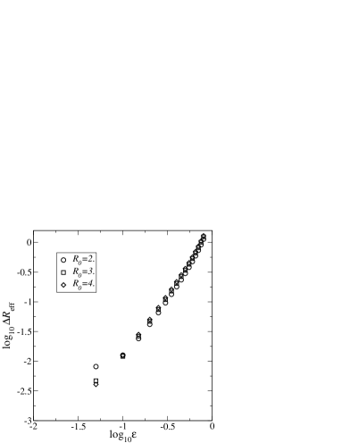
Figure 1: Logarithm of the “effective radial dispersion” $\Delta R_{\text{eff}}(t=0)$ vs. eccentricity $\varepsilon$ for the ansatz (4). $\Delta R_{\text{eff}}$ is clearly a good measure of asymmetry, increasing always monotonically with $\varepsilon$.

The asymmetry in the initial field configuration is introduced by means of an elliptical deformation:

$$\phi(\rho,\theta,0)=-2\exp\left[-\frac{r^{2}(\rho,\theta)}{R_{0}^{2}}\right]+1,$$ (4)

where:

$$r^{2}(\rho,\theta)=\frac{\rho^{2}}{1-\varepsilon^{2}\cos^{2}\theta},$$ (5)

with $\varepsilon:[0,1)$ the bubble eccentricity, $R_{0}$ the bubble “radius” and $\rho,\theta$ polar coordinates (notice that this expression reduces to the usual symmetric ansatz when $\varepsilon=0$). We note in passing that a similar parameterization was adopted in the study of eccentric pulsons in the sine-Gordon theory chris .

Figure 2: Oscillon energy in a shell of radius $R_{s}=5R_{0}$ for $R_{0}=2.0$ and $0.1\leq\varepsilon\leq 0.8$, from bottom to top (only integer multiples of $\varepsilon=0.1$ are shown).

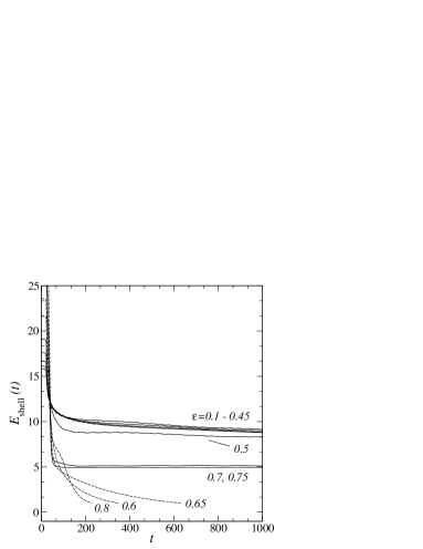
Figure 3: Oscillon energy in a shell of radius $R_{s}=5R_{0}$, now for $R_{0}=3.0$ and $0.1\leq\varepsilon\leq 0.8$, with steps $\Delta\varepsilon=0.05$. Dashed lines indicate unstable configurations.

In order to measure the asymmetry of the field configuration, we take advantage of the effective radius $R_{\text{eff}}$ defined in Ref. osc2 and introduce an “effective radial dispersion” $\Delta R_{\text{eff}}$ (see below). The effective radius could be recast in the form:

$$R_{\text{eff}}(t)\equiv\langle R(\theta,t)\rangle_{\theta},$$ (6)

where $\langle\cdot\rangle_{\theta}=(2\pi)^{-1}\int_{0}^{2\pi}{\text{d}}\theta$ is an angular average and $R(\theta,t)$ is a $\theta$-dependent effective radius defined by (compare Eq. (28) of Ref. osc2 ):

$$R(\theta,t)=\frac{\int_{0}^{R_{\text{s}}}{\text{d}}\rho~{}\rho^{2}\left[\frac{1}{2}(\nabla\phi)^{2}+V(\phi)\right]}{(2\pi)^{-1}\int_{0}^{2\pi}{\text{d}}\theta\int_{0}^{R_{\text{s}}}{\text{d}}\rho~{}\rho\left[\frac{1}{2}(\nabla\phi)^{2}+V(\phi)\right]},$$ (7)

with $R_{\text{s}}$ the “shell radius” (i.e. the radius within which we integrate all the quantities relative to the oscillon). This notation allows us to construct angular averages and dispersions in a manner analogous to time averages. We therefore define the effective radial dispersion as the relative root-mean-square deviation from the average radius:

$$\Delta R_{\text{eff}}(t)\equiv\frac{\sqrt{\langle R^{2}(\theta,t)\rangle_{\theta}-\langle R(\theta,t)\rangle_{\theta}^{2}}}{\langle R(\theta,t)\rangle_{\theta}}.$$ (8)

As shown in Figure 1, the above quantity is indeed a good measure of asymmetry, i.e. it increases monotonically with $\varepsilon$. It is approximately independent of the bubble size, being the limiting case $\Delta R_{\text{eff}}=0$ an indication of a symmetrical state (though not exactly zero on a lattice due to its finite resolution). We now turn to the presentation of the main numerical experiments obtained by solving Eq. (3) with the initially asymmetrical bubbles (4) for eccentricities $\varepsilon$ ranging from $0.1$ to $0.8$ and $R_{0}$ from $2.0$ to $5.0$. This investigation can easily be extended to greater values of $R_{0}$, although this would require much longer computational times without generating results of much physical interest. [The computational time ${\mathcal{C}}_{\text{time}}$ is proportional to $L^{2}$, which in turn is proportional to $(R_{0})^{2}$, see Appendix].

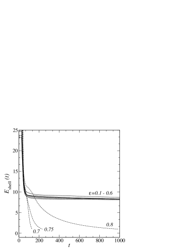
Figure 4: Oscillon energy for $R_{0}=4.0$ and different $\varepsilon$, with steps $\Delta\varepsilon=0.05$ (dashed lines are for unstable configurations).

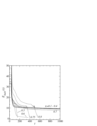
Figure 5: Shell energy for bubbles of radius $R_{0}=5.0$ and steps $\Delta\varepsilon=0.05$ (dashed lines for unstable cases).

Figures 2-5 show the time evolution of the total energy within a shell of radius $R_{\text{s}}=5R_{0}$ surrounding the initial configuration for different values of $R_{0}$ and $\varepsilon$. It is seen that, in general, initially asymmetric bubbles tend to decay into coherent field configurations with an approximately constant energy plateau similar to those found in Ref. sornb , which focused on the evolution of symmetric configurations. With the help of the effective radial dispersion $\Delta R_{\text{eff}}$, we can investigate whether these configurations correspond to “excited” states of an oscillon (i.e., non-spherically symmetric configurations analogous to an excited state of a hydrogen atom for $\ell\neq 0$) or if the bubble asymmetry is completely lost and the system decays into a “ground” (i.e. symmetric) state.

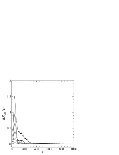
Figure 6: $\Delta R_{\text{eff}}$ for $R_{0}=4.0$ and $0.1\leq\varepsilon\leq 0.6$, from bottom to top (only integer multiples of $\varepsilon=0.1$ are shown). Notice how the initial asymmetric bubble decays into a circularly symmetric configuration.

In Fig. 6 we show the time evolution of $\Delta R_{\text{eff}}$ for the $R_{0}=4.0$ case. It is clearly seen that the initially asymmetric bubble decays into a $\Delta R_{\text{eff}}=0$, symmetric configuration, after a brief asymmetric pulsation. A similar pattern was observed for all initial radii investigated here, suggesting that whenever an oscillon stage is set, the resulting configuration is circularly symmetric. The peaks in this figure also suggest that $\Delta R_{\text{eff}}$ might follow a scaling law for different values of $\varepsilon$. Indeed, a collapse of these curves using the scaling $\Delta R_{\text{eff}}(\varepsilon,t)=\varepsilon^{\alpha}f(t),$ where $\alpha$ is a real constant and $f(t)$ is a function of time only, is shown in Figure 7.

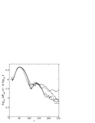
Figure 7: Collapse of $\Delta R_{\text{eff}}$ in Figure 6 using $\Delta R_{\text{eff}}(\varepsilon,t)=\varepsilon^{\alpha}f(t)$ for $\alpha\approx 2.05$. Note that the time domain is restricted to $t\leq 250$, since $\Delta R_{\text{eff}}\rightarrow 0$ for $t\gtrsim 250$ (causing the log scale to be ill behaved).

As the reader must have noticed, an intriguing feature of these results is the presence of some “instability windows” for some values of $\varepsilon$. These can be observed here in the cases $R_{0}=3.0$ and $R_{0}=5.0$. Thus, oscillons do not always appear as the asymmetric configurations decays. A finer investigation of the parameter space for the elliptical deformations, generalizing what was done in great detail for spherically-symmetric 3+1 dimensional oscillons honda , will quite possibly reveal a very rich and detailed substructure of stable and unstable windows. It is important to stress that once $\Delta R_{\rm eff}\rightarrow 0$ (cf. fig. 6), the field does settle into an oscillon, as the phase space portrait of Fig. 8 exemplifies. This justifies our earlier claim that oscillons are attractors in field-configuration space.

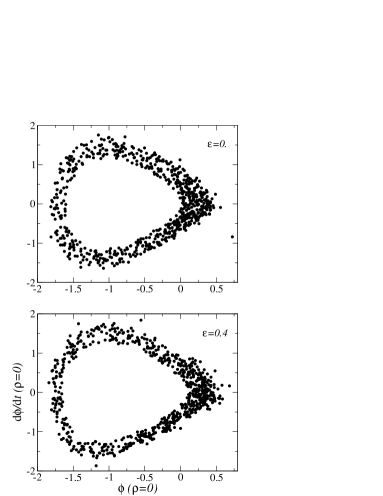
Figure 8: Phase portrait between $t=0$ and $t=1000$ at $\rho=0$ of a bubble entering an oscillon stage for $R_{0}=2.0$ and $\varepsilon=0$ (top) and $\varepsilon=0.4$ (bottom): the symmetric configuration to which asymmetric bubbles decay is an oscillon.

A crucial step not yet studied is the stability analysis against small but arbitrary asymmetric perturbations. The oscillon stability with regard to these perturbations is fundamental for the computation of quantum corrections around the classical solution rajaraman ; lee and is the subject of the next session.

III Stability analysis

Our task now is to investigate whether symmetric oscillons are stable against small radial and angular perturbations $\delta\phi(\rho,\theta,t)$, i.e. to probe the “linear stability” of the oscillon. We are unaware of any previous study where the stability of a field configuration with a time-dependent amplitude has been tested against small fluctuations. So far, stability investigations have been restricted to either time-independent configurations, such as bounce solutions coleman2 , or to configurations with a linear time-dependence in the phase, such as $Q$-balls coleman ). The stability analysis in these two situations is greatly simplified by the fact that the dynamical equation dictating the behavior of the fluctuations is separable into its spatial and temporal parts; the resulting problem reduces to finding the eigenvalues $\omega_{n}^{2}$ of a time-independent operator (an alternative approach based on the so-called “Bogomolnyi bound” bogomolnyi can also be applied in the time-independent case, see e.g. calberto ). The existence of at least one negative eigenvalue $\omega_{n}^{2}$ (and thus of a complex eigenfrequency $\omega_{n}$) signals the presence of an exponentially-growing instability jackiw (a well-known example is the so-called “bounce” solution, which we will investigate further below coleman2 ). The present problem, however, is not amenable to such treatment due to the anharmonic time-dependence of the oscillon; we must consider both the space- and time-dependence of the background field, making the stability analysis of oscillon-type configurations considerably more challenging both analytically and numerically, as we will now discuss.

In order to appreciate these difficulties, let us write (in polar coordinates) the linearized equation of motion that follows from Eq. (3) through the substitution $\phi(\rho,\theta,t)\rightarrow\phi_{0}(\rho,t)+\delta\phi(\rho,\theta,t)$, where $\phi_{0}$ is the symmetric oscillon solution and $\delta\phi\ll\phi_{0}$ is the perturbation, i.e.,

$$\frac{\partial^{2}}{\partial t^{2}}\delta\phi=\frac{\partial^{2}}{\partial\rho^{2}}\delta\phi+\frac{1}{\rho}\frac{\partial}{\partial\rho}\delta\phi+\frac{1}{\rho^{2}}\frac{\partial^{2}}{\partial\theta^{2}}\delta\phi-(3\phi_{0}^{2}-1)\delta\phi.$$ (9)

Here one might be tempted to separate the variables as $\delta\phi\equiv R(\rho)\Theta(\theta)T(t)$. However, the resulting equations show that one cannot get rid of the simultaneous radial and temporal dependence of the background configuration, $\phi_{0}(\rho,t)$ . This situation should be contrasted to the usual case where $\phi_{0}$ is a time-independent solution, e.g. the bounce, or to the case where the time-dependence of $\phi_{0}$ is in a phase factor $\exp(i\omega t)$, and thus immediately eliminated in the full equation of motion coleman . A considerable simplification can nevertheless be accomplished by writing $\delta\phi\equiv\Phi(\rho,t)\Theta(\theta)$, isolating at least the angular part of the problem. Performing such substitution gives the pair of equations,

$$\ddot{\Phi}-\Phi^{\prime\prime}-\frac{1}{\rho}\Phi^{\prime}+\left(U_{0}(\rho,t)+\frac{\ell^{2}}{\rho^{2}}\right)\Phi=0,$$ (10)

and

$$\frac{d^{2}\Theta(\theta)}{d\theta^{2}}=-\ell^{2}\Theta(\theta),$$ (11)

with overdots and primes indicating time and radial derivatives, respectively. Here $U_{0}(\rho,t)\equiv 3\phi_{0}^{2}-1$ and $\ell$ is a separation constant. The solutions for $\Theta$ are trivial, viz. $\Theta\propto\exp(\pm i\ell\theta)$, and by requiring $\delta\phi$ to be single-valued we have $\ell=0,1,2,...$. Our original (2+1)-dimensional problem, Eq. (9), reduces therefore to solving the above (1+1)-dimensional one, Eq. (10), since the time-dependence is present only in $\Phi$.

Our goal is to probe the linear stability of the oscillon by solving Eq. (10) for arbitrary initial conditions. The strategy is to monitor the time evolution of the perturbations $\delta\phi$, which should grow without bounds in the case of a linearly unstable configuration merkin ; morrison . An obvious limitation of this approach is that it is impossible to scan all initial values of perturbations, viz. $\delta\phi(\rho,0)$ with $\ell=0,1,2,...$. The method thus is only indicative of stability, not being able to provide conclusive proof. The more thorough the search, the more one is guaranteed to show stability, at least against most types of perturbation. This unavoidable limitation should be contrasted with the simpler case for time-independent background configurations based on a harmonic decomposition $T(t)\propto\exp(i\omega_{n}t)$ (see e.g. coleman ; jackiw ), where the existence of exponentially unstable modes is clearly related to imaginary eigenvalues. However, we would like to point out a limitation of the spectral method that is often overlooked. By restricting the analysis to an exponential time-dependence, as in $T(t)$ above, one can obtain only spectral instabilities of a configuration, leaving aside other possible forms of instabilities, for example, linear (or power-law) ones. In other words, a system that is spectrally stable may still be unstable against slower growing modes morrison ; lichtenberg . Since we are here essentially watching the full time-dependence of $\delta\phi$, we should be able to detect any sort of instability by observing its long-time behavior, although in practice the infinite-time limit or a complete scan of possible fluctuations cannot be achieved numerically. Fortunately, we shall shortly see that typical spectral instabilities (such as that of the bounce) do not require a long-time integration or a very wide search, being therefore bound to be observed through our method. Before we do so, it is worth testing the reliability of the numerical implementation itself.

III.1 Linear test

The first step is to compare the numerical solution of Eq. (10) with a closed-form analytical one in order to prepare and test our numerical implementation, since the singular behavior at the origin requires a careful treatment. This can be done most easily by setting $U_{0}(\rho,t)=0$, in which case Eq. (10) becomes linear and separable, with $\Phi=R(\rho)T(t)$. This gives $T\propto\exp(\pm i\omega t)$, where $\omega$ is a separation constant, and the equation for $R$,

$$R^{\prime\prime}+\frac{1}{\rho}R^{\prime}+\left(\omega^{2}-\frac{\ell^{2}}{\rho^{2}}\right)R=0,$$ (12)

which we recognize as Bessel’s equation. By requiring regularity at the origin and $\dot{\Phi}(\rho,0)=0$, the solution can be written as

$$\Phi_{\ell}(\rho,t)=\int_{0}^{\infty}\!\!d\omega f(\omega)J_{\ell}(\omega\rho)\cos(\omega t),$$ (13)

where $f(\omega)$ is determined by the initial condition. Choosing $\Phi(\rho,0)=AJ_{\ell}(a\rho)$ we have

$$f(\omega)=A\omega\int_{0}^{\infty}\!\!d\rho\,\rho J_{\ell}(a\rho)J_{\ell}(\omega\rho)=A\delta(\omega-a),$$ (14)

and therefore

$$\Phi_{\ell}(\rho,t) = A\int_{0}^{\infty}\!\!d\omega\,\delta(\omega-a)J_{\ell}(\omega\rho)\cos(\omega t)$$ (15)

$$= AJ_{\ell}(a\rho)\cos(at).$$

The above solution maintains its shape but oscillates harmonically with period $2\pi/a$. We have verified that our numerical implementation reproduces correctly this analytical solution for various values of $a$ and $\ell$.

Figure 9: Semi-log plot of the maximum amplitude $\Phi_{max}$ versus time for the bounce solution (showing here three different initial conditions). The slope denotes the common unstable mode eigenvalue, $\omega_{n}$.

III.2 The bounce

As a first application of our method we investigate the stability of the so-called “bounce” solution coleman2 , which is guaranteed to be spectrally unstable in any dimension greater than (1+1) due to Derrick’s theorem derrick . (In fact, Coleman has showed that only one negative eigenvalue exists coleman3 ). Should our method be reliable, the solution $\delta\phi$ for the case where $\phi_{0}$ is a bounce solution will grow exponentially at late times, indicating the presence of an unstable mode.

The bounce solution $\phi_{b}(\rho)$ is the $O(2)$-symmetric static configuration that solves the equation

$$\frac{d^{2}\phi}{d\rho^{2}}+\frac{1}{\rho}\frac{d\phi}{d\rho}=V^{\prime}(\phi),$$ (16)

with the asymmetric potential

$$V(\phi)=\frac{\beta}{2}\phi^{2}-\frac{1}{3}\phi^{3}+\frac{1}{4}\phi^{4}.$$ (17)

In order to detect the instability, we solved Eq. (10) with $U_{0}(\rho)=\beta-2\phi_{b}(\rho)+3\phi_{b}^{2}(\rho)$ and various initial conditions, sweeping the lattice at every time step to find the maximum value of the perturbation, $\Phi_{max}$. In Fig. 9, we show our results for $\beta=0.011$ [the initial conditions are Eq. (18) with $n=0,1$ and $m=2$, and Eq. (20) for $m=2$, both with $\ell=0$]; one can clearly identify the exponential growth of $\delta\phi$ even at early times $t<100$. Also shown is the slope of the curve, which should match the unstable eigenvalue $\omega_{n}$ obtained with the usual spectral method. [We have attempted to obtain such eigenvalue by solving numerically the associated Schrödinger-like equation. However, in two spatial dimensions the severe singularity at the origin causes a numerical instability which we were unable to control even with sophisticated methods liu . Since this is not the focus of this paper, we will leave this question aside.]

III.3 The oscillon

We are now ready to apply our method to the stability of the oscillon, which was obtained here by solving Eq. (3) with the symmetrical version ($\varepsilon=0$) of the ansatz Eq. (4). We have essentially followed the same procedure described above for the bounce, but now evolving both $U_{0}$ and $\Phi$ in Eq. (10). Since the dimensionality of the configuration space is infinite, we chose arbitrarily the initial profiles of the fluctuations $\Phi(\rho,t_{0})$, with the only constraint that they should vanish at $\rho\rightarrow\infty$ to ensure localization around the oscillon. The time $t_{0}$ was chosen to be about $200$, since that is roughly when the initial bubbles have just decayed into an oscillon (cf. Figs. 2-5). Some examples of the initial configurations investigated here are

$$\Phi_{\ell}(\rho,t_{0}) =x^{n}\exp\left(-\frac{\rho^{m}}{R_{0}^{m}}\right),$$ (18)

$$\Phi_{\ell}(\rho,t_{0}) =\sin\left(\frac{2n\pi\rho}{R_{0}}\right)\exp\left(-\frac{\rho^{m}}{R_{0}^{m}}\right),$$ (19)

$$\Phi_{\ell}(\rho,t_{0}) =J_{\ell}(\rho)\exp\left(-\frac{\rho^{m}}{R_{0}^{m}}\right),$$ (20)

for various integer values of $n,m$ and $\ell$ (namely, $n=0,1,2$, $m=2,3$ and $\ell=0,1,2,3$).

Figure 10: A typical outcome of the linear stability analysis of the oscillon, showing here $\Phi_{max}$ vs. time for $\ell=0$, $n=0$ and $m=2$ in Eq. (18). The radius of the initial bubble is $R_{0}=2$.

In Figure 10 we show a typical outcome of our search. In all cases investigated we found that the fluctuations $\Phi_{max}$ are bounded from above, as one would expect from a linearly stable configuration. We conclude that if, indeed, there are any unstable modes, they are sufficiently slow-growing to justify the use of the oscillon as a stable bound state. [We have integrated the linearized equations of motion up to $t=10^{4}$; see also discussion below]. Note that the large amplitude of $\Phi$, e.g. $\sim 1000$ in Fig. 10, does not mean that the condition $\delta\phi\ll\phi_{0}$ is violated: since the resulting equation is linear, any solution can always be rescaled without changing its shape by choosing a different constant prefactor for the initial conditions.

Although not as systematic and transparent as the investigation above, another approach to check the stability of oscillons is to superimpose the perturbation to the full (2+1)-dimensional oscillon dynamics discussed in Sec. II. One can then probe the oscillon stability simply by checking the persistence of the energy plateau: if the added energy from the perturbations is radiated away, the oscillon is stable. Due to the dimensionality of the problem, the numerical treatment is quite more challenging than the one use above within the linear method. Nevertheless, we have investigated the stability of oscillons against superimposed fluctuations for similar initial conditions. In Fig. 11 we present the outcome of a particular choice of initial condition for three different initial radii. The results are consistent with the previous stability analysis, as can be seen by the persistence of the energy plateau.

On the basis of our extensive search with many different initial conditions and long integration times, we find it very unlikely that an exponentially-growing mode exists. If it does, it would be either very small and/or related to a very “rare” excitation; the oscillon configuration would still be stable for large times and could be considered a legitimate (or at least a very long-lived) bound state in semi-classical quantization.

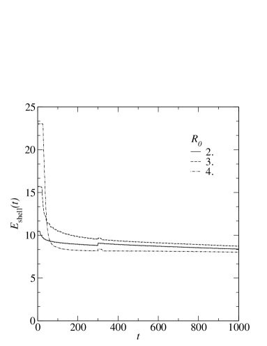
Figure 11: An example of the full dynamics of the oscillon when subject to a perturbation of the form in Eq. (18) for $n=0$ and $m=2$ at $t=300$. The maximum amplitude of the initial perturbation - here the prefactor in Eq. (18) - was constrained to either $0.01$ or $0.05$, although the results do not change appreciably even for $0.1$. The stability is evident through the persistence of the energy plateau.

IV Conclusions

We have investigated, in 2+1 dimensions, two key questions concerning the properties of oscillons – time-dependent, localized field configurations that emerge during the deterministic evolution of $\phi^{4}$ models. First, we have shown that initially asymmetric configurations evolve, for a wide range of elliptic deformations, into symmetric oscillons states. Thus, oscillons are not just particular to symmetric initial states. This result led us to propose that oscillons are attractors in field configuration space, with a very deep attractor basin, at least in 2+1 dimensions. Second, we have shown that oscillons are stable against a wide range of asymmetric small perturbations. This result was obtained by two distinct approaches, one solving the linearized equation for the perturbations and the other by superimposing the perturbations on the oscillons and evolving the perturbed configurations with the full equation of motion. Clearly, both methods are restricted to the choice of initial fluctuations. However, after an extensive search, we were unable to find any unstable fluctuation with either approach. To the best of our knowledge, this is the first dynamical investigation of the stability of explicitly time-dependent scalar field configurations. We expect that both of these results will carry on to 3+1 dimensions, although probably the attractor basin will be shallower in this case.

These results suggest the importance time-dependent spatio-temporal structures may have in a wide range of physical systems, from condensed matter to early universe cosmology. Although we have restricted our study to simple $\phi^{4}$ models, we expect, as suggested in Refs. osc2 ; sornb , that oscillons will be present whenever there is a bifurcation instability related to the negative curvature of the nonlinear potential. Oscillons will emerge in a wide variety of dynamical systems, possibly representing a bottleneck to equipartition of energy, thus delaying the approach to equilibrium.

One possible arena for oscillons in early universe cosmology is during the reheating supposed to occur after inflation. Oscillons may be thermally nucleated with a probability proportional to $\exp[-E_{\rm osc}/T]$, where $E_{\rm osc}$ is the energy of the oscillon configuration. They will act as “entropy sinks”, confining several degrees of freedom to an ordered state, delaying the thermalization of the universe. Eventually, when they decay into radiation, they will dump more entropy to the early universe, possibly changing the final reheating temperature.

Finally, it would be interesting to compute the spectrum of quantum fluctuations around oscillon states, to investigate their effect on oscillon stability. Time-dependent bound states may have much to add to our knowledge of nonperturbative quantum field theory, which has traditionally focused on time-independent configurations, such as instantons.

*

Appendix A Numerical method

The integration scheme adopted here is a standard leapfrog algorithm, which ensures second-order precision in time numrec (the spatial discretization used is fourth-order). We have adopted the “adiabatic damping method” (or simply the damping method) of Ref. sornb together with Higdon’s first-order boundary conditions higdon . Their combined use turned out to be very effective and of easy implementation, allowing us to tackle this otherwise demanding numerical problem with current workstations.

Put briefly, the leapfrog equations with the damping method read:

$$\dot{\phi}^{n+1/2}_{i,j} = \frac{(1-\eta_{i,j}\Delta t/2)\dot{\phi}^{n-1/2}_{i,j}+\Delta t[\nabla^{2}\phi^{n}_{i,j}-V^{\prime}(\phi^{n}_{i,j})]}{1+\eta_{i,j}\Delta t/2},$$

$$\phi^{n+1}_{i,j} = \phi^{n}_{i,j}+\Delta t\dot{\phi}^{n+1/2}_{i,j},$$ (21)

where superscripts (subscripts) denote temporal (spatial) indices, $\eta_{i,j}$ is the damping function of Ref. sornb and $V^{\prime}(\phi)$ is a first partial derivative of the potential with respect to the field. The second spatial derivatives in the Laplacian are discretized with a fourth-order scheme (to wit, $\partial_{xx}\phi_{i,j}\approx[16(\phi_{i+1,j}+\phi_{i-1,j})-\phi_{i+2,j}-\phi_{i-2,j}-30\phi_{i,j}]/12\Delta x^{2}$ and analogously for $\partial_{yy}\phi_{i,j}$), which gives an energy conservation of one part in $10^{3}$ for $\Delta x=0.1$ and $\Delta t=0.06$ (and, of course, with $\eta_{i,j}\equiv 0$). A better energy conservation could be obtained with smaller $\Delta x$ or $\Delta t$, but this comes with a high price tag since, as remarked below, the computational time is inversely proportional to both $\Delta x^{2}$ and $\Delta t$. Despite this fact, with the above parameters we were able to reproduce quite accurately the results of Gleiser and Sornborger sornb . Even though the damping method is already a major improvement over more naive methods (such as huge lattices or even moving boundary conditions), for the problem at hand it is still demanding. As an example, for small oscillons of radius $R_{0}\approx 2.0$, the required lattice of radial dimension $R\approx 200$ adopted in Ref. sornb (and thus $L\approx 400$ in our square grid, where $L$ is the lattice edge), would already demand a total of $N\sim 10^{7}$ sites for $\Delta x=0.1$, as opposed to the $N\sim 10^{3}$ used in the latter reference. Another aggravating fact comes from the large integration times $\tau$ involved in such problems [notice that the required computational time for this problem goes roughly as ${\mathcal{C}}_{\text{time}}\sim(\tau/\Delta t)N=(\tau/\Delta t)(L/\Delta x)^{2}$]. We note in passing that there has been some effort to find a more natural and efficient discretization for the $\phi^{4}$ theory which might reduce significantly the computational time of such problems speight . Motivated by this possibility, two of us have recently investigated these lattices and have found that, unfortunately, they are of limited practical use even for simple dynamical problems kinkdyn . It was seen, however, that if the above scheme is supplied with the boundary conditions of Ref. higdon :

$$\left.\left(\partial_{t}\pm\partial_{\alpha}\right)\phi\right|_{\partial\Omega}=0,$$ (22)

where $\alpha$ is either $x$ or $y$, then a significantly smaller lattice could be used, resulting in an energy error smaller than (or equal to) the error due to numerical energy fluctuations. [These first-order “absorbing boundary conditions” were obtained for the rather simple (linear) wave equation. We expect, however, that the damping introduced before the boundaries could reduce the amplitude of the outgoing waves such that Eq. (3) is effectively linearized in that region, and thus that the boundary condition (22) becomes applicable]. With regard to the example in the previous paragraph, we have found that the required lattice with this “mixed” method needs only $L\approx 140$ (in contrast to the former $L\approx 400$), such that $N$ (and thus ${\mathcal{C}}_{\text{time}}$) is roughly one order of magnitude smaller than the previous one (this trend is also found for greater $R_{0}$). For the sake of completeness, we quote here the parameters of the damping method used throughout our simulations (we use the same functional form for $\eta(\rho)$ as Ref. sornb ): $k=0.005$ (damping constant), $\rho_{0}=10R_{0}$ (initial radius of the damping) and $\rho_{\ell}=50$ (damping length), these latter two being defined such that $L=2(\rho_{0}+\rho_{\ell})$.

We expect that the method adopted here might be useful not only in higher dimensional systems (the two methods above do not really make any dimensional requirement), but also in other finite-domain problems not necessarily related to oscillons.

References

- (1) R. Rajaraman, Solitons and Instantons (North-Holland, Amsterdam, 1987).
- (2) T. D. Lee and Y. Pang, Phys. Rep. 221, 251 (1992).
- (3) S. Coleman, Nucl. Phys. B262, 263 (1985).
- (4) A. Kusenko, Nucl. Phys. B (Proc. Suppl.) 62A/C, 248 (1998); A. Kusenko, M. Shaposhnikov, and P. Tinyakov, Pisma Zh.Eksp.Teor.Fiz. 67, 229 (1998); JETP Lett. 67, 247 (1998); M. Axenides, E. Floratos, and A. Kehagias, Phys. Lett. B 444, 190 (1998).
- (5) J. A. Frieman, G. B. Gelmini, M. Gleiser, and E. W. Kolb, Phys. Rev. Lett. 60, 2101 (1988); J. A. Frieman, A. V. Olinto, M. Gleiser, and C. Alcock, Phys. Rev. D 40, 3241 (1989); R. Friedberg, T. D. Lee, and Y. Pang, ibid. 35, 3658 (1987), and references therein. More recently, important consequences of NTS and balls in cosmology were advanced by A. Kusenko and M. Shaposhnikov, Phys. Lett. B 418, 46 (1998); A. Kusenko, V. Kuzmin, and M. Shaposhnikov, P. G. Tinyakov, Phys. Rev. Lett. 80, 3185 (1998); K. Enqvist and J. McDonald, Phys. Lett. B 425, 309 (1998). D. Metaxas, Phys. Rev. D 63, 083507 (2001); A. Kusenko and P. J. Steinhardt, Phys. Rev. Lett. 87, 141301 (2001).
- (6) M. Gleiser, Phys. Rev. D 49, 2978 (1994).
- (7) E. J. Copeland, M. Gleiser and H.-R. Muller, Phys. Rev. D 52, 1920 (1995). Oscillons at finite temperature were investigated by M. Gleiser and R. M. Haas, Phys. Rev. D 54, 1626 (1996).
- (8) S. Flach and C. R. Willis, Phys. Rep. 295, 181 (1998); D. K. Campbell, J. F. Schonfeld, and C. A. Wingate, Physica 9D, 1 (1983).
- (9) M. Gleiser and A. Sornborger, Phys. Rev. E 62, 1368 (2000).
- (10) P. L. Christiansen, N. Gronbech-Jensen, P. S. Lomdahl, and B. A. Malomed, Phys. Scripta 55, 131 (1997).
- (11) E. Honda and M. Choptuik, Phys. Rev. D 68, 084037 (2002).
- (12) E. B. Bogomol’nyi, Sov. J. Nucl. Phys. 24, 449 (1976).
- (13) F. S. A. Cavalcante, M. S. Cunha, and C. A. S. Almeida, Phys. Lett. B 475, 315. (2000).
- (14) R. Jackiw, Rev. Mod. Phys. 49, 681 (1977).
- (15) S. Coleman, Phys. Rev. D 15, 2929 (1977).
- (16) D. R. Merkin, Introduction to the Theory of Stability (Springer, New York, 1997).
- (17) P. J. Morrison, Rev. Mod. Phys. 70, 467 (1998).
- (18) A. J. Lichtenberg, M. A. Lieberman, Regular and Chaotic Dynamics, 2nd Ed. (Springer, New York, 1992).
- (19) G. H. Derrick, J. Math. Phys. 5, 1252 (1964).
- (20) S. Coleman, Aspects of Symmetry, Cambridge University Press (Cambridge, UK 1985).
- (21) X. Liu, L. Su, P. Ding, Int. J. Quant. Chem. 87, 1 (2002).
- (22) W. H. Press, et al., Numerical Recipes, 2nd Ed. (Cambridge University Press. News York, 1992).
- (23) G. B. Arfken and H. J. Weber, Mathematical Methods for Physicists, 4th Ed. (Academic Press, 1995).
- (24) R. L. Higdon, Math. Comp. 47 (1986), 437.
- (25) J. M. Speight, Nonlinearity 10, 1615 (1997). See also: J. M. Speight and R. Ward, Nonlinearity 8, 517 (1994); J. M. Speight, Nonlinearity 12, 1373 (1999).
- (26) A. B. Adib and C. A. S. Almeida, Phys. Rev. E 64, 037701 (2001).