Scalar fields: from domain walls to nanotubes and fulerenes

Abstract

In this work we review some features of topological defects in field theory models for real scalar fields. We investigate topological defects in models involving one and two or more real scalar fields. In models involving a single field we examine two different subclasses of models, which support one or more topological defects. In models involving two or more real scalar fields, we explore the presence of defects that live inside topological defects, and junctions and networks of defects. In the case of junctions of defects we investigte structures that simulate nanotubes and fulerenes. Our investigations may also be used to describe nonlinear properties of polymers, Langmuir films and optical solitons in fibers.

]

I Introduction

Research on topological defects in Field Theory was iniciated almost three decades ago, and some of the main investigations may be found for instance in Refs. [1, 2, 3, 4, 5]. In the case of topological defects that appears in models described by real scalar fields in $(1,1)$ space-time dimensions, they are usually named kinks, and are classical static solutions of the equations of motion. Their topological behavior is related to the asymptotic form of the field configurations, which has to differ in both the positive and negative space directions. To ensure that the classical solutions have finite energy, one requires that the asymptotic behavior of the solutions is identified with minima of the potential that defines the system under consideration, so in general the potential has to include at least two distinct minima for the system to support topological solutions.

We can investigate real scalar fields in $(3,1)$ space-time dimensions, and now the topological solutions are named domain walls. These domain walls are bidimensional structures that carry surface tension, which is identified with the energy of the classical solutions that spring in $(1,1)$ space-time dimensions. The domain wall structures are supposed to play a role in applications to several different contexts, ranging from the low energy scale of condensed matter [6, 7, 8] up to the high energy scale required in the physics of elementary particles, fields and cosmology [1, 2, 3, 4, 5].

There are at least three classes of models that support kinks or domain walls. In the first class one deals with a single real scalar field, and the topological solutions are structureless. Examples of this are the sine-Gordon and $\phi^{4}$ models. In the second class of models one also deals with a single real scalar field, but now the systems comprise at least two distinct domain walls. An example of this is the double sine-Gordon model, which has been investigated for instance in Refs. [9, 10, 11]. In the third class of models we deal with systems defined by two real scalar fields, and now one opens two new possibilities: domain walls that admit internal structure [12, 13, 14, 15, 16, 17, 18, 19, 20], and junctions of domain walls, which appear in models of two fields when the potential contains non-colinear minima, as recently investigated for instance in Refs.[21, 22, 23, 24, 25, 26, 27, 28, 29, 30, 31, 32, 33, 34, 35].

There are other motivations to investigate domain walls in models of field theory, one of them being related to the fact that the low energy world volume dynamics of branes in string and M theory may be described by standard models in field theory [36, 37, 38]. Besides, one knows that field theory models of scalar fields may also be used to investigate properties of quasi-linear polymeric chains, as for instance in the applications of Refs. [39, 40, 41, 42], to describe solitary waves in ferroelectric crystals, the presence of twistons in polyethylene, and solitons in Langmuir films.

In the present work, in Sec. II we review some known facts about models described by real scalar fields. The investigations follow in Secs. III and IV, where we search for topological structures that generate kinks and walls, in models involving a single real scalar field, and two or more fields, respectively.

II General Considerations

In this work we are interested in field theory models that describe real scalar fields and support topological solutions of the Bogomol’nyi-Prasad-Sommerfield (BPS) type [43, 44]. In the case of a single real scalar field $\phi$, we consider the Lagrange density

$${\cal L}=\frac{1}{2}\partial_{\alpha}\phi\partial^{\alpha}\phi-V(\phi)$$ (1)

Here $V(\phi)$ is the potential, which identifies the particular model under consideration. We write the potential in the form $V(\phi)=(1/2)\,W^{2}_{\phi}$, where $W=W(\phi)$ is a smooth function of the field $\phi$, and $W_{\phi}=dW/d\phi$. In a supersymmetric theory $W$ is the superpotential, and this is the way we name $W$ in this work.

The equation of motion for $\phi=\phi(x,t)$ has the general form

$$\frac{\partial^{2}\phi}{\partial t^{2}}-\frac{\partial^{2}\phi}{\partial x^{2}}+\frac{dV}{d\phi}=0$$ (2)

and for static solutions we get

$$\frac{d^{2}\phi}{dx^{2}}=W_{\phi}W_{\phi\phi}$$ (3)

It was recently shown in Ref. [45] that this equation of motion is equivalent to the first order equations

$$\frac{d\phi}{dx}=\pm W_{\phi}$$ (4)

if one is searching for solutions that obey the boundary conditions $\lim_{x\to-\infty}\phi(x)={\bar{\phi}}_{i}$ and $\lim_{x\to-\infty}(d\phi/dx)=0$, where ${\bar{\phi}}_{i}$ is one among the several vacua $\{{\bar{\phi}}_{1},{\bar{\phi}}_{2},...\}$ of the system. In this case the topological solutions are BPS (+) and anti-BPS (-) solutions. Their energies get minimized to the value $t^{ij}=|\Delta W_{ij}|$, where $\Delta W_{ij}=W_{i}-W_{j}$, with $W_{i}$ standing for $W({\bar{\phi}}_{i})$. The BPS and anti-BPS solutions are defined by two vacuum states belonging to the set of minima that identify the several topological sectors of the model.

In the case of two real scalar fields $\phi$ and $\chi$ the potential is written in terms of the superpotential, in a way such that $V(\phi,\chi)=(1/2)\,W^{2}_{\phi}+(1/2)\,W^{2}_{\chi}$. The equations of motion for static fields are

$$\frac{d^{2}\phi}{dx^{2}}=W_{\phi}W_{\phi\phi}+W_{\chi}W_{\chi\phi}$$ (5)

$$\frac{d^{2}\chi}{dx^{2}}=W_{\phi}W_{\phi\chi}+W_{\chi}W_{\chi\chi}$$ (6)

which are solved by the first order equations

$$\frac{d\phi}{dx}=\pm W_{\phi}\,\;\;\;\;\;\;\;\;\frac{d\chi}{dx}=\pm W_{\chi}$$ (7)

Solutions to these first order equations are BPS (+) and anti-BPS (-) states. They solve the equations of motion, and have energy minimized to $t^{ij}=|\Delta W^{ij}|$ as in the case of a single field; here, however, $\Delta W^{ij}=W(\phi_{i},\chi_{i})-W(\phi_{j},\chi_{j})$, since now we need a pair of numbers $(\phi_{i},\chi_{i})$ to represent each one of the vacuum states in the system of two fields. In the plane $(\phi,\chi)$ we may have minima that are non colinear, openning the possibility for junctions of defects. In the case of two real scalar fields, we can find a family of first order equations that are equivalent to the pair of second order equations of motion, but this requires that the superpotential is harmonic, obeying $W_{\phi\phi}+W_{\chi\chi}=0$ [45].

III Models involving a single real scalar field

We now turn attention to kinks and domain walls. A well known example is given by the $\phi^{4}$ model, defined by the potential $V(\phi)=(1/2)\,(\phi^{2}-1)^{2}$. Here we are using natural units, and dimensionless fields and coordinates. In this model the domain wall can be represented by the solution $\phi_{s}(x)=\pm\tanh(x)$. The above potential can be written with the superpotential $W(\phi)=\phi-\phi^{3}/3$, and the domain wall is of the BPS or anti-BPS type. The wall tension corresponding to the BPS wall is $t_{s}=4/3$.

We can also find structureless domain walls in other models, for instance in the $\phi^{6}$ model, which is described by the potential $V(\phi)=(1/2)\,\phi^{2}\,(\phi^{2}-1)^{2}$. Here we have $W(\phi)=(1/2)\phi^{2}-(1/4)\phi^{4}$, and the wall configurations are also of the BPS type, and are given by ${\bar{\phi}}^{2}_{s}=(1/2)[1\pm\tanh(x)]$. The wall tension is now ${\bar{t}}_{s}=1/4$. This potential was investigated for instance in Ref. [46].

We can build another class of models where the domain walls engender other features. The next class is yet described by a single field, but the systems may now support two or more different walls. An interesting example of this is the double sine-Gordon model, which is defined by the potential

$$V_{r}(\phi)=\frac{1}{r+1}\bigl{[}4\,r\,\cos(\phi)+\cos(2\phi)\bigr{]}$$ (8)

where $r$ is a parameter, real and positive. This potential is periodic, with period $2\pi$; for simplicity in the following we consider the interval $-2\pi<\phi<2\pi$. The value $r=1$ distinguishes two regions, the region $r\in(0,1)$ where the potential contains four minima, and the region $r\geq 1$, where the potential contains two minima. For $r\in(0,1)$ the system supports two distinct wall configurations, the large wall and the small wall, which distinguish the two different barrier the model comprises in this case. The limits $r\to 0$ and $r\to\infty$ lead us back to the sine-Gordon model. The double sine-Gordon model has been considered in several distinct applications, as for instance in Ref. [9, 10, 11], where one investigates magnetic solitons in superfluid ³He, kink propagation in a model for poling in polyvinylidine fluoride, and properties related to the two different kinks that appear in such polymeric chain.

To expose new features of the double sine-Gordon model we rewrite Eq. (8) in the form [47]

$$V_{r}(\phi)=\frac{2}{1+r}[\cos(\phi)+r\,]^{2}$$ (9)

where we have omitted an unimportant r-dependent constant. The model can be described by the superpotential

$$W(\phi)=\frac{2}{\sqrt{1+r}}[\sin(\phi)+r\,\phi]$$ (10)

For $r$ in the interval $r\in(0,1)$ the minima of the potential are the singular points of the superpotential, $dW/d\phi=0$. They are periodic, and for $-2\pi<\phi<2\pi$ there are four minima, at the points ${\bar{\phi}}=\pm\pi\pm\,\alpha(r)$, where $\alpha(r)=\cos^{-1}(r)$. For $r\geq 1$ the minima are at ${\bar{\phi}}=\pm\pi$, in the interval $-2\pi<\phi<2\pi$. A closer inspection shows that for $0<r<1$ the local maxima at $\pm\pi$ and the minima $\pm\pi\pm\alpha(r)$ degenerate to the minima $\pm\pi$ for $r=1$, and remain there for $r>1$. Thus, the parameter $r$ induces a transition in the behavior of the double sine-Gordon model. The value $r=1$ is the critical value, since it is the point where the system changes behavior: for $r\in(0,1)$ this model supports minima that desapear for $r\geq 1$. We illustrate the double sine-Gordon model in Fig. 1, where we depict the potential of Eq. (9) for $r=1/3,2/3$ and for $r=1$.

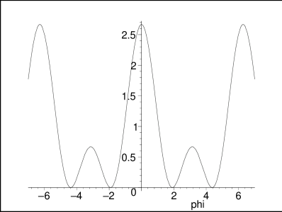
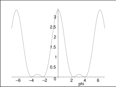
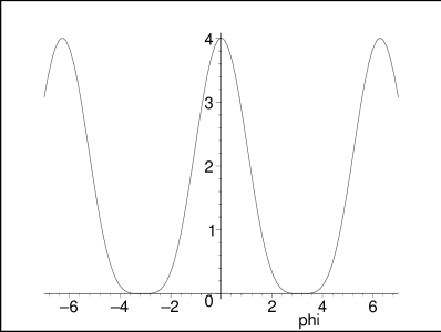
FIG. 1.: The double sine-Gordon potential, depicted for $r=1/3,2/3$ and $1$ from above to below respectively, to illustrate how the behavior of the model changes with $r$.

We get a better view of the phase transition in the double sine-Gordon model by examining the order parameter ${\bar{\phi}}(r)$, which is given by $\pm\pi\pm\,\alpha(r)$ for $0<r\leq 1$, so it goes continuously to $\pm\pi$ for $r\geq 1$. Also, the (squared) mass of the field can be obtained via the relation

$$V_{r}^{\prime\prime}({\bar{\phi}})=W^{2}_{{\bar{\phi}}{\bar{\phi}}}+W_{{\bar{\phi}}}W_{{\bar{\phi}}{\bar{\phi}}{\bar{\phi}}}$$ (11)

where ${\bar{\phi}}$ is the corresponding minimum of the potential. For $0<r\leq 1$ we get $m^{2}(r)=4-4r$, and for $r\geq 1$ we have $m^{2}(r)=4(r-1)/(r+1)$. We plot ${\bar{\phi}}(r)$ and $m^{2}(r)$ in Fig. 2. We see that $m(r)$ vanishes in the limit $r\to 1$. These results indicate that $r$ drives a second order phase transition, a transition where the system goes from the case of two distinct phases to another one, engendering a single phase.

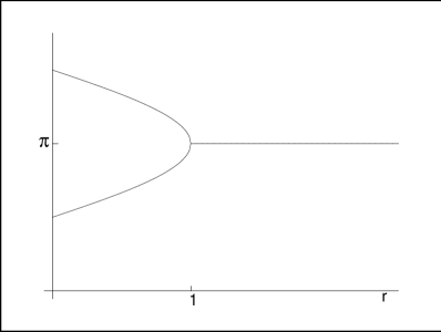
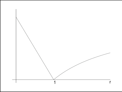
FIG. 2.: Plots of ${\bar{\phi}}(r)$ (above) and $m^{2}(r)$ (below) for the double sine-Gordon potential, which illustrate how the behavior of the model changes with $r$.

We consider $0<r\leq 1$. The energies of the BPS solutions are given as follows. For solutions connecting the minima $-\pi+\alpha(r)$ and $\pi-\alpha(r)$ the defect is large since it joins minima separated by a higher and wider barrier. We have

$$t^{l}_{dsG}=4\sqrt{1-r}+4r\frac{\pi-\alpha(r)}{\sqrt{1+r}}$$ (12)

In the case of the minima $\pi-\alpha(r)$ and $\pi+\alpha(r)$ the defect is small and we get

$$t^{s}_{dsG}=4\sqrt{1-r}-4r\frac{\alpha(r)}{\sqrt{1+r}}$$ (13)

We notice that $t^{l}_{dsG}=t^{s}_{dsG}+4\pi r/\sqrt{1+r}$, and that the limit $r\to 1$ sends $t^{l}_{dsG}\to 2\sqrt{2}\pi$ and $t^{s}_{dsG}\to 0$, as expected. For the BPS states we can write the solutions explicitly. For instance, for solutions that connect the minima $-\pi+\alpha(r)$ and $\pi-\alpha(r)$ we get large kink solutions, which are of the form

$$\phi_{l}(x)=\pm 2\tan^{-1}\Biggl{[}\sqrt{\frac{1+r}{1-r}}\,\tanh\left(\sqrt{1-r}\;x\right)\Biggr{]}$$ (14)

For solutions that connect the minima $\pi\pm\alpha(r)$ and the minima $-\pi\pm\alpha(r)$ we get small kink solutions. They are given by

$$\phi_{s}(x)=\pm\pi-2\tan^{-1}\Biggl{[}\sqrt{\frac{1-r}{1+r}}\,\tanh\left(\sqrt{1-r}\,x\right)\Biggr{]}$$ (15)

The potential in Eq. (9) in the limit $r\to 0$ goes to

$$V_{0}(\phi)=1+\cos(2\phi)$$ (16)

which leads us back to the sine-Gordon model. Thus, we can suppose $r$ small and use $V_{r}(\phi)$ to explore the double sine-Gordon model as a model controlled by a small parameter, in the vicinity of the sine-Gordon model. This feature may be of some use for investigations that follow the lines of Ref. [48], and also in the case concerning the presence of internal modes of solitary waves, which seems to appear when one slightly modifies some integrable model – see for instance Ref. [49].

IV Models involving two or more real scalar fields

We now turn attention to the third class of models, which is described by two real scalar fields. In this case the domain walls may engender internal structure. This line of investigation follows as in Refs. [14, 15, 16] and we illustrate such possibility with the system defined by the potential

$$V(\phi,\chi) = \frac{1}{2}(\phi^{1}-1)^{2}+\frac{1}{2}r^{2}\left(\chi^{2}-\frac{1}{r}\right)^{2}+$$ (18)

$$r(1+2r)\phi^{2}\chi^{2}$$

where the parameter $r\neq 0$ is real. This model was first investigated in Ref. [50], and can be used to modify the internal structure of domain walls – see Refs. [16, 51]. This potential follows from the superpotential

$$W(\phi,\chi)=\phi-\frac{1}{3}\phi^{3}-r\phi\chi^{2}$$ (19)

and the system supports two-field solutions. An explicit solution is

$$\phi(x) = \tanh(2rx)$$ (20)

$$\chi(x) = a(r)\,{\rm sech}(2rx)$$ (21)

with $a^{2}(r)=1/r-2$. This is a BPS solution, and now the parameter $r$ is restricted to the interval $r\in(0,1/2)$. The limit $r\to 1/2$ lead us to the one-field solution $\phi(x)=\tanh(x)$ and $\chi(x)=0$. As we know, all the BPS solutions are linearly stable [52].

The two-field solutions obey

$$\phi^{2}+\chi^{2}/a^{2}=1$$ (22)

which describes an elliptic arc connecting the two minima $(\pm 1,0)$ of the corresponding potential in the $(\phi,\chi)$ plane. The one-field solutions represent standard domain walls, while the two-field solutions may be seen as domain walls having internal structure: the vector $(\phi,\chi)$ in configuration space describes an straight line segment for the one-field solution, and an elliptic arc for the two-field solution, resembling light in the linearly and elliptically polarized cases, respectively. The same solutions appear in condensed matter, in the anysotropic $XY$ model used to describe ferromagnetic transition in magnetic systems, and there they are named Ising and Bloch walls, respectively – see for instance Ref. [8], chapter 7.

We recall that domain walls may be seen as seeds [4, 5] for the formation of non-topological structures. This possibility appears in Refs. [53, 54, 55, 56], where the discrete symmetry is changed to an approximate symmetry, or in Ref. [57], with the discrete symmetry biased so that domains of distinct but degenerate vacua spring unequally. Domain walls that appear in models involving two real scalar fields present features that are not seen in the case of a single field. Thus, we are now investigating other extensions of the above model, defined by the superpotential of Eq. (19). In the work in Ref. [58] we are investigating the possibility of changing the elliptic arc to a more general orbit, that may find applications in condensed matter. In another work [59] we are investigating other superpotentials, non-polynomial, in an effort to extend the model studied in [60, 61, 62] to the case of two or more fields. The model defined by the superpotential of Eq. (19) present other interesting features, recently explored in Ref. [63], which deserve further investigations.

We now turn our attention to polynomial potentials that engenders the $Z_{3}$ symmetry, and that supports stable three-junctions that generate a regular hexagonal network of defects. Investigations on the presence of junctions [64] of defects in supersymmetric models have been given in Refs. [21, 22, 23], and in Ref. [25] we have found the fourth-order polynomial potential

$$V(\phi,\chi) = \lambda^{2}\phi^{2}\left(\phi^{2}-\frac{9}{4}\right)+\lambda^{2}\chi^{2}\left(\chi^{2}-\frac{9}{4}\right)$$ (24)

$$+\,2\,\lambda^{2}\,\phi^{2}\,\chi^{2}-\lambda^{2}\phi\,(\phi^{2}-3\,\chi^{2})+\frac{27}{8}\lambda^{2}$$

This potential does not allow for supersymmetric extensions. The equations of motion for static configurations that follows in this case are

$$\frac{d^{2}\phi}{dx^{2}} = \lambda^{2}\phi\left(4\phi^{2}+4\chi^{2}-3\,\phi-\frac{9}{2}\right)+3\lambda^{2}\chi^{2}$$ (25)

$$\frac{d^{2}\chi}{dx^{2}} = \lambda^{2}\chi\left(4\phi^{2}+4\chi^{2}+6\,\phi-\frac{9}{2}\right)$$ (26)

The potential has three degenerate minima, at the points $v_{1}=(3/2)\,(1,0)$ and $v_{2,3}=(3/4)\,(-1,\pm\sqrt{3})$. These minima form an equilateral triangle, invariant under the $Z_{3}$ symmetry. The distance between the minima is $(3/2)\sqrt{3}$.

We can obtain the topological solutions explicitly. The easiest way to do this follows by first examining the sector that connects the vacua $v_{2}$ and $v_{3}$. This is so because in this case we set $\phi=-3/4$, searching for a strainght-line segment in the $(\phi,\chi)$ plane. This is compatible with the Eq. (25), and reduces the other Eq. (26) to the form

$$\frac{d^{2}\chi}{dx^{2}}=\lambda^{2}\left(4\chi^{3}-\frac{27}{4}\chi\right)$$ (27)

This implies that the orbit connecting the vacua $v_{2}$ and $v_{3}$ is a straight line. It is such that, along the orbit the $\chi$ field feels the potential $\lambda^{2}\,[\chi^{2}-(27/16)]^{2}$. This shows that the model reduces to a model of a single field, and the solution satisfies the first-order equation

$$\frac{d\chi}{dx}=\sqrt{2}\lambda\left(\chi^{2}-\frac{27}{16}\right)$$ (28)

The solution is

$$\chi(x)=-\frac{3}{4}\sqrt{3}\tanh\left(\sqrt{\frac{27}{8}}\lambda\,x\right)$$ (29)

The other solutions can be obtained by rotations obeying the $Z_{3}$ symmetry of the model.

The full set of solutions of the equations of motion are collected below. In the sector connecting the minima $v_{2}$ and $v_{3}$ they are

$$\phi^{(\pm)}_{(2,3)} = -\frac{3}{4}$$ (30)

$$\chi^{(\pm)}_{(2,3)} = \pm\frac{3}{4}\sqrt{3}\,\tanh\left(\sqrt{\frac{27}{8}}\,\lambda\,x\right)$$ (31)

In the sector connecting the minima $v_{1}$ and $v_{2}$ they are

$$\phi^{(\pm)}_{(1,2)} = \frac{3}{8}\pm\frac{9}{8}\,\tanh\left(\sqrt{\frac{27}{8}}\,\lambda\,x\right)$$ (32)

$$\chi^{(\pm)}_{(1,2)} = \frac{3}{8}\sqrt{3}\mp\frac{3}{8}\sqrt{3}\,\tanh\left(\sqrt{\frac{27}{8}}\,\lambda\,x\right)$$ (33)

In the sector connecting the minima $v_{1}$ and $v_{3}$ they are

$$\phi^{(\pm)}_{(1,3)} = \frac{3}{8}\mp\frac{9}{8}\,\tanh\left(\sqrt{\frac{27}{8}}\,\lambda\,x\right)$$ (34)

$$\chi^{(\pm)}_{(1,3)} = -\frac{3}{8}\sqrt{3}\mp\frac{3}{8}\sqrt{3}\,\tanh\left(\sqrt{\frac{27}{8}}\,\lambda\,x\right)$$ (35)

The label $(\pm)$ is used to identify kink and antikink. All the solutions have the same energy, $(9/4)\,\sqrt{27/8}\,|\lambda|$.

We examine how the bosonic fields behave in the background of the classical solutions. We do this by considering fluctuations around the static solutions $\phi(x)$ and $\chi(x)$. We use the equations of motion to see that the fluctuations depend on the potential

$${\bf U}(x)={{V_{\phi\phi}\,\,\,V_{\phi\chi}}\choose{V_{\chi\phi}\,\,\,V_{\chi\chi}}}$$ (36)

Evidently, after obtaining the derivatives we substitute the fields by their classical static values $\phi(x)$ and $\chi(x)$. The model under consideration is defined by the potential (50). In this case we use (30) and (31) to obtain two decoupled equations for the fluctuations. The potentials of the corresponding Schrödinger-like equations are

$$U_{11}(x) = \frac{27}{8}\lambda^{2}\Biggl{[}4-2\,{\rm sech}^{2}\left(\sqrt{\frac{27}{8}}\lambda\,x\right)\Biggr{]}$$ (37)

$$U_{22}(x) = \frac{27}{8}\lambda^{2}\Biggl{[}4-6\,{\rm sech}^{2}\left(\sqrt{\frac{27}{8}}\lambda\,x\right)\Biggr{]}$$ (38)

The eigenvalues can be obtained explicitly: in the $\chi$ direction we get $w^{\chi}_{0}=0$ and $w^{\chi}_{1}=(9/2)\sqrt{\lambda^{2}/2}$, and in the $\phi$ direction we have $w^{\phi}_{0}=(9/2)\sqrt{\lambda^{2}/2}$. This shows that the pair $(\ref{sol11})$ and $(\ref{sol12})$ is stable, and by symmetry we get that all the three topological solutions are stable solutions.

The classical solutions present the nice property of having energy evenly distributed in their gradient (g) and potential (p) portions. In terms of energy density they are

$${\rm g}(x)={\rm p}(x)=\frac{1}{4}\left(\frac{27}{8}\right)^{2}\,\lambda^{2}\,{\rm sech}^{4}\left(\sqrt{\frac{27}{8}}\lambda\,x\right)$$ (39)

To understand this feature we recall the calculation done explicitly in the sector with $\phi=-3/4$, constant. There the model is shown to reduce to a model of a single field, a model that supports BPS solutions. Within this context, the above solutions are very much like the non-BPS solutions that appear in supersymmetric systems [26]. We use this property and the topological current

$$J^{\alpha}=\varepsilon^{\alpha\beta}\partial_{\beta}{\phi\choose\chi}$$ (40)

It obeys $\partial_{\alpha}J^{\alpha}=0$, and it is also a vector in the $(\phi,\chi)$ plane. For static configurations we have $J^{t}_{\alpha}\,J^{\alpha}=\rho^{t}\,\rho$, where $\rho=\rho(\phi,\chi)$ is the charge density. This charge density allows writing $\rho^{t}\rho=\varepsilon(x)$, where $\varepsilon(x)={\rm g}(x)+{\rm p}(x)$ is the (total) energy density of the solution. We use this result and the notation $ij$, to identify the sector connecting the vacua $(\phi_{i},\chi_{i})$ and $(\phi_{j},\chi_{j})$, to show that for any two different sectors $ij$ and $jk$, $i,j,k=1,2,3$ we get that

$$(\rho_{ij}+\rho_{jk})^{t}\,(\rho_{ij}+\rho_{jk})<\rho_{ij}^{t}\rho_{ij}+\rho_{jk}^{t}\rho_{jk}$$ (41)

This condition shows that the three-junction is a process of fusion of defects that occurs exothermically, providing stability of junctions in the present model. This result is more general than the one in Ref. [64], which appears within the context of supersymmetry. Evidently, our result also works for BPS and non-BPS solutions that appears in supersymmetric models, with the property of having energy evenly distributed in their gradient and potential portions [26].

We notice that the orbits corresponding to the stable defect solutions form an equilateral triangle in the $(\phi,\chi)$ plane. This is so because the solutions are straight-line segments joining the three vacuum states in configuration space. They are degenerate in energy, and this allows associating to each defect the same tension

$$t=\frac{9}{4}\,\sqrt{\frac{27}{8}}\,\,|\lambda|$$ (42)

This makes $t_{ij}<t_{jk}+t_{ki},i,j,k=1,2,3$, and now the inequality is strictly valid in this case, stabilizing the three-junction that appears in this model when one enlarges the space-time to three spatial dimensions.

We consider the possibility of junctions in the plane, which may give rise to a planar network of defects. We work in $(2,1)$ space-time dimensions, in the plane $(x,y)$. We identify the plane $(x,y)$ with the space of configurations, the plane $(\phi,\chi)$. We illustrate this situation by considering, for instance, the solutions we have already obtained. They are collected in Eqs. (30)-(35) in (1,1) dimensions. In the planar case they change to

$$\phi^{(\pm)}_{(2,3)} = -\frac{3}{4}$$ (43)

$$\chi^{(\pm)}_{(2,3)} = \pm\frac{3}{4}\sqrt{3}\tanh\left(\sqrt{\frac{27}{8}}\,\lambda\,y\right)$$ (44)

and

$$\phi^{(\pm)}_{(1,2)} = \frac{3}{8}\mp\frac{9}{8}\tanh\left(\frac{1}{2}\sqrt{\frac{27}{8}}\,\lambda\,(y+\sqrt{3}x)\right)$$ (45)

$$\chi^{(\pm)}_{(1,2)} = \frac{3}{8}\sqrt{3}\pm\frac{3}{8}\sqrt{3}\tanh\left(\frac{1}{2}\sqrt{\frac{27}{8}}\,\lambda\,(y+\sqrt{3}x)\right)$$ (46)

and

$$\phi^{(\pm)}_{(1,3)} = \frac{3}{8}\pm\frac{9}{8}\tanh\left(\frac{1}{2}\sqrt{\frac{27}{8}}\,\lambda\,(y-\sqrt{3}x)\right)$$ (47)

$$\chi^{(\pm)}_{(1,3)} = -\frac{3}{8}\sqrt{3}\pm\frac{3}{8}\sqrt{3}\tanh\left(\frac{1}{2}\sqrt{\frac{27}{8}}\,\lambda\,(y-\sqrt{3}x)\right)$$ (48)

These planar defects are domain walls, and can be used to represent the three-junction in the limit of thin walls.

The three-junction that appears in this $Z_{3}$-symmetric model allows building a network of defects, precisely in the form of a regular hexagonal network, as depicted in Fig. 3 in the thin wall approximation. In this network the tension associated to the defect is the tipical value of the energy in this tiling of the plane with a regular hexagonal network, which seems to be the most efficient way of tiling the plane. As we have shown, our model behaves standardly in $(3,1)$ dimensions. It supports stable three-junctions that generate a stable regular hexagonal network of defects.

FIG. 3.: A regular hexagonal network of defects, formed by three-junctions surrounded by domains representing the vacua $v_{1}=1,v_{2}=2$, and $v_{3}=3$.

In Ref. [25] the idea of nesting a network of defects inside a domain wall has been presented. A model that contains the basic mechanisms behind this idea was introduced in Ref. [31]. It is described by three real scalar fields $\sigma$, $\phi$, and $\chi$, and is defined by the (dimensionless) potential,

$$V(\sigma,\phi,\chi) = \frac{2}{3}\,\left(\sigma^{2}-\frac{9}{4}\right)^{2}+\left(r\,\sigma^{2}-\frac{9}{4}\right)\,(\phi^{2}+\chi^{2})$$ (50)

$$+(\phi^{2}+\chi^{2})^{2}-\phi\,(\phi^{2}-3\,\chi^{2})$$

Here $r$ couples $\sigma$ to the pair of fields $(\phi,\chi)$. This potential is polynomial, and contains up to the fourth order power in the fields. Thus, it behaves standardly in $(3,1)$ space-time dimensions. Also, it presents discrete $Z_{2}\times Z_{3}$ symmetry. We set $(\phi,\chi)\to(0,0)$, to get the projection $V(\sigma,0,0)\to V(\sigma)=(2/3)\,(\sigma^{2}-9/4)^{2}$. The projected potential presents $Z_{2}$ symmetry, and can be written with the superpotential $W(\sigma)=(2\sqrt{3}/9)\sigma^{3}-(3\sqrt{3}/2)\sigma$, in the form $V=(1/2)(dW/d\sigma)^{2}$. The reduced model supports the explicit configurations $\sigma_{h}(z)=\pm\,(3/2)\,\tanh(\sqrt{3}z)$. The tension of the host wall is $t_{h}=3\,\sqrt{3}=(3/2)\,m_{h}$, where $m_{h}$ represents the mass of the elementary $\sigma$ meson. Also, the width of the wall is such that $l_{h}\sim 1/\sqrt{3}$.

The potentials projected inside $(\sigma\to 0)$ and outside $(\sigma\to\pm\,3/2)$ the host domain wall are $V_{in}(\phi,\chi)$ and $V_{out}(\phi,\chi)$. Inside the wall we have

$$V_{in}(\phi,\chi) = (\phi^{2}+\chi^{2})^{2}-\phi\,(\phi^{2}-3\,\chi^{2})$$ (52)

$$-\frac{9}{4}(\phi^{2}+\chi^{2})+\frac{27}{8}$$

This potential engenders the $Z_{3}$ symmetry, and there are three global minima, at the points $v^{in}_{1}=(3/2)(1,0)$ and $v^{in}_{2,3}=(3/4)(-1,\pm\sqrt{3})$, which define an equilateral triangle. Outside the wall we get

$$V_{out}(\phi,\chi) = (\phi^{2}+\chi^{2})^{2}-\phi\,(\phi^{2}-3\,\chi^{2})$$ (54)

$$+\frac{9}{4}\,(r-1)\,(\phi^{2}+\chi^{2})$$

$V_{out}$ also engenders the $Z_{3}$ symmetry, but now the minima depend on $r$. We can adjust $r$ such that $r>9/8$, which is the condition for the fields $\phi$ and $\chi$ to develop no non-zero vacuum expectation value outside the host domain wall, ensuring that the model supports no domain defect outside the host domain wall. The restriction of considering quartic potentials forbids the possibility of describing the $Z_{3}$ portion of the model with the complex superpotential used in [21].

We investigate the masses of the elementary $\phi$ and $\chi$ mesons. Inside the wall they degenerate to the single value $m_{in}=3\sqrt{3/2}$. Outside the wall, for $r>9/8$ they also degenerate to a single value, $m_{out}(r)=3\sqrt{(r-1)/2}$, which depends on $r$. We see that $m_{out}(r=4)=m_{in}$. Also, $m_{out}(r)>m_{in}$ for $r$ bigger than 4, and $m_{out}(r)<m_{in}$ for $r$ in the interval $(9/8,4)$.

We study linear stability of the classical solutions $\sigma=\sigma_{h}(z)$ and $(\phi,\chi)=(0,0)$. The fields $\phi$ and $\chi$ vanish classically, and their fluctuations $(\eta_{n},\xi_{n})$ decouple. The procedure leads to two equations for the fluctuations, that degenerate to the single Schrödinger-like equation

$$-\,\frac{d^{2}\psi_{n}(z)}{dz^{2}}+\frac{9}{2}\,V(z)\;\psi_{n}(z)=\,w_{n}^{2}\,\psi_{n}(z)$$ (55)

Here $V(z)=-1+r\,\tanh^{2}{\sqrt{3}z}$. This equation is of the modified Pöschl-Teller type, and can be examined analytically. The lowest eigenvalue is $w_{0}^{2}=(3/2)\sqrt{6\,r+1\,}-6$. There is instability for $r<5/2$, showing that the host domain wall with $(\phi,\chi)=(0,0)$ is unstable and therefore relax to lower energy configurations, with $(\phi,\chi)\neq(0,0)$ for $r<5/2$. Inside the host domain wall the sigma field vanishes, and the model is governed by the potential $V_{in}(\phi,\chi)$, which consequently may allow the presence of non-trivial $(\phi,\chi)$ configurations. The host domain wall entraps the system described by $V_{in}(\phi,\chi)$ for the parameter $r$ in the interval $(9/8,5/2)$. In this interval we have $m_{out}<m_{in}$, showing that it is not energetically favorable for the elementary $\phi$ and $\chi$ mesons to live inside the wall for $r\in(9/8,5/2)$. The model automatically suppress backreactions of the $\phi$ and $\chi$ mesons into the defects that may appear inside the host domain wall.

In Ref. [25] the potential inside the wall was shown to admit a network of domain walls, in the form of a hexagonal array of domain walls. In the thin wall approximation the network may be represented by the solutions

$$\phi_{{}_{1}} = \frac{3}{8}+\frac{9}{8}\tanh\left(\frac{1}{2}\sqrt{\frac{27}{8}}\,(y+\sqrt{3}x)\right)$$ (56)

$$\chi_{{}_{1}} = \frac{3}{8}\sqrt{3}-\frac{3}{8}\sqrt{3}\tanh\left(\frac{1}{2}\sqrt{\frac{27}{8}}\,(y+\sqrt{3}x)\right)$$ (57)

and by $(\phi_{k},\chi_{k})$, obtained by rotating the pair $(\phi_{1},\chi_{1})$ by $2(k-1)\pi/3$, for $k=2,3$. We identify the space $(\phi,\chi)$ with $(x,y)$, so rotations in $(\phi,\chi)$ also rotates the plane $(x,y)$ accordingly. The energy or tension of the individual defects in the network is given by, in the thin wall approximation, $t_{n}=(27/8)\sqrt{3/2}=(9/8)\;m_{in}$. In the nested network, the width of each defect obeys $l_{n}\sim\sqrt{8/27}$. This shows that $l_{h}/l_{n}=3/2\sqrt{2}$, and so the host domain wall is slightly thicker than the defects in the nested network. In the thin wall approximation, the potential $V_{in}(\phi,\chi)$ allows the formation of three-junctions as reactions that occur exothermically, and the nested array of thin wall configurations is stable. In Fig. 4 we depict the hexagonal network of defects inside the domain wall, in the thin wall approximation; the dashed lines show equilateral triangles, that belong to the dual lattice. Both the hexagonal network and the dual triagular network are composed of equilateral polygons, a fact that follows in accordance with the $Z_{3}$ symmetry.

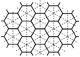
FIG. 4.: The equilateral hexagonal network of defects, that may live inside the host domain wall. The dashed lines show the dual lattice, formed by equilateral triangles.

We now explore the breaking of the $Z_{2}\times Z_{3}$ symmetry of the model. The simplest case refers to the breaking of the $Z_{3}$ symmetry, without breaking the remaining $Z_{2}$ symmetry. We consider the case of breaking the internal $Z_{3}$ symmetry in the following way. We take for instance the vacuum state $v_{1}^{in}=(3/2)\,(1,0)$, and change its position to a location farther from or closer to the other minima of the system, increasing or decreasing the angle between two of the three defects; see Fig. 5. We can do this with the inclusion in the potential of another term, proportional to the second-order power on $\phi$. We notice that the energy of the defect depends on the distance between the two minima the defect connects, and goes with the cube of it. Thus, if the vacuum state deviates significantly from its $Z_{3}$-symmetric position, we cannot neglect the correction to the energy of the defects. This changes the regular hexagonal pattern of Fig. 4 to two other hexagonal patterns, composed of thicker or thinner hexagons. We recall that hexagonal patterns may appear in chemical systems [65], and in fluid convection [66] where they may also involve non-equilateral hexagons.

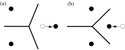
FIG. 5.: The vacuum states (black dots) and the junction that forms the nested network. (a) and (b) illustrate the only two ways of breaking the $Z_{3}\to Z_{2}$ symmetry.

We explore the presence of local defects in the hexagonal network by introducing penta-hepta pair of cells, in a local deformation of the network that disorganize its otherwise regular pattern. The mechanism is similar to that of Refs. [67, 68]. However, if the $Z_{2}$ symmetry that governs the host domain wall is effective, local deformations may only appear in a flat surface, requiring the pentagons and heptagons are not regular polygons. This possibility may be seen in Bénard-Marangoni convection; see Ref. [69] for a report on the experimental observation of such paterns. But if together with the slight breaking of the $Z_{3}$ symmetry of the internal network, one slightly breaks the $Z_{2}$ symmetry of the host domain wall locally, this will ultimately favor the appearence of local deformations composed of pair of equilateral pentagons and heptagons. Since in the network of equilateral hexagons, the presence of equilateral pentagons and heptagons introduce local curvature, positive and negative, respectively, we can understand these local defects as a mechanism for roughening the planar surface that contains the network. To break the symmetry of the nested network, one requires a slight change of position of one of the three minima of the nested system, so we can neglect the difference in energy and consider the tension as in the regular hexagonal network. We see that the roughening springs to generate higher energy states from the planar regular hexagonal structure.

We now concentrate on breaking the $Z_{2}$ symmetry of the host domain wall. We can do this with the inclusion in the potential of a term odd in $\sigma$, that slightly removes the degeneracy of the two minima $\sigma=\pm 3/2$. Thus, the host domain wall bends trying to involve the local minimum, the false vacuum. To stabilize the non-topological structure we include charged fields into the system. The way one couples the charged fields is not unique, but if we choose to add fermions, we can couple them to the $\sigma$ field in a way such that the projection with $(\phi,\chi)\to(0,0)$ may leave the model supersymmetric. This is obtained with the superpotential $W(\sigma)$, with the Yukawa coupling $d^{2}W/d\sigma^{2}=(4/3)\sqrt{3}\,\sigma$. In this case massless fermions bind [70] to the host domain wall, and contribute to stabilize [56] the non-topological defect that emerges with the breaking of the $Z_{2}$ symmetry.

The breaking of the $Z_{2}$ symmetry can be done breaking or not the remaining $Z_{3}$ symmetry of the model. We examine these two possibilities supposing that the host domain wall bends under the assumption of spherical symmetry, becoming a non-topological defect with the standard spherical shape. This is the minimal surface of genus zero, and according to the Euler theorem we can only tile the spherical surface with three-junctions as a regular polygonal network in the three different ways: with 4 triangles, or 6 squares, or yet 12 pentagons. They are the tetrahedron, cube, and dodecahedron, respectively. They are three of the five different ways of tiling the sphere with regular polygons, known as the Platonic solids [71]. These three cases preserve the $Z_{3}$ symmetry of the original network, locally, at the three-junction points. However, if locally one slightly breaks the $Z_{3}$ symmetry of the network to the $Z_{2}$ one, the three-junctions can now tile the spherical surface with 12 pentagons and 20 hexagons. We think of breaking the $Z_{3}$ symmetry minimally, to the $Z_{2}$ symmetry, through the same mechanism presented in Fig. 5. Thus, if the symmetry is broken slightly we can consider the defect tensions as in the regular hexagonal network.

The tiling with 12 pentagons and 20 hexagons generates a spherical structure that resembles the fullerene, the buckyball composed of sixty carbon atoms [72, 73]. This is the truncated icosahedron, one among thirteen different possibilities of tiling the sphere with regular polygons of two or more distinct types, known as the Archimedean solids [71]. The truncated icosahedron is one of the seven Archimedean solids constructed with triple junctions, and it is the one that breaks the $Z_{3}$ symmetry very slightly. We visualize the symmetries involved in the spherical structures thinking of the corresponding dual lattices, which are triangular lattices, but in the three first cases the triangles are equilateral, while in the fourth case they are isosceles. We recall that regular heptagons introduce negative curvature, so they cannot appear when the genus zero surface is minimal. However, they may for instance spring to generate higher energy states from the fullerene-like structure, locally roughening the otherwise smooth spherical surface.

We write the energy of the non-topological structure as $E^{n}_{nt}=E^{s}_{nt}+E_{n}$, where $E^{s}_{nt}$ stands for the energy of the standard non-topological defect, and $E_{n}$ is the portion due to the nested network. We use $E^{s}_{nt}=E_{q}+E_{h}$, which shows the contributions of the charged fields and of the host domain wall, respectively. We have $E_{h}=S\,t_{h}$, and $E_{n}=N\,d\,t_{n}$, where $S$ is the area of the spherical surface, and $N$ and $d$ are the number and length of segments in the nested network. We introduce the ratio $E^{n}_{nt}/E^{s}_{nt}=1+[N/(1+r)](t_{n}/t_{h})(d/S)$, with $r=E_{q}/E_{h}$. The non-topological structure nests a network of defects, which modifies the scenario one gets with the standard domain wall. The modification depends on the way one couples charged bosons and fermions to the $\sigma,\phi$, and $\chi$ fields. However, if the $Z_{3}$ symmetry is locally broken to the $Z_{2}$ one, the most probable defect corresponds to the fullerene or buckyball structure. But if the $Z_{3}$ symmetry is locally effective, there may be three equilateral structures, the most probable arising as follows. We consider the simpler case of plane polygonal structures, identifying the tetrahedron ($i=3$), cube ($i=4$), and dodecahedron ($i=5$). We introduce $r_{ij}$ as the energy ratio for the $i$ and $j$ structures. We get $r_{ij}=(1+r+t_{n}/h_{i}\,t_{h})/(1+r+t_{n}/h_{j}\,t_{h})$, for $i,j=3,4,5$. Here $h_{3},h_{4}$, and $h_{5}$ stand for the radius of the incircle of the triangle, square, and pentagon, respectively. Energy favors the triangular lattice as the nested network. This configuration is self-dual, because the network and its dual are the very same triangular lattice. The two other configurations (that add to give the five Platonic solids) are the octahedron, dual to the cube, and the icosahedron, dual to the dodecahedron. They do not appear in the $Z_{2}\times Z_{3}$ model because they require four- and five-junctions, respectively.

Our work can be extended in several directions. For instance, we could use the $Z_{2}\times Z_{k}$ symmetry $(k=4,5,6)$, getting to $k$-junctions. This allows to tile the plane with squares $(k=4)$, or triangles $(k=6)$, and the spherical surface with triangles, as the octahedron $(k=4)$ or the icosahedron $(k=5)$. This direction seems appropriate to model the recent experimental observations of squares in specific Rayleigh-Bénard and Bénard-Marangoni convections [74, 75]. Also, in the $Z_{2}\times Z_{3}$ model, if the host domain wall bends cylindrically, one may get to nanotube-like configurations [76, 77]. As one knows, in certain types of nanotubes one can find polarons [78], so we are using this idea to investigate the presence of chiral polarons in chiral nanotubes. Another line of investigations concern the use of real scalar fields to map laser beams interacting inside nonlinear fiber optics, as for instance in the model we have already presented in Ref. [79], where laser beams that generate black solitons are used to give rise to a vector soliton of the black and bright type.

We would like to thank C.A.G. Almeida, B. Baseia, F.A. Brito, W. Freire, L. Losano, J.M.C. Malbouisson, J.R.S. Nascimento, R.F. Ribeiro, M.M. Santos, and C. Wotzasek for invaluable discussions, and CAPES, CNPq, PROCAD and PRONEX for financial support.

REFERENCES

- [1] R. Rajaraman, Solitons and Instantons (North-Holland, Amsterdam, 1982).
- [2] C. Rebbi and Soliani, Solitons and Particles (World Scientific, Singapore, 1984).
- [3] S. Coleman, Aspects of Symmetry (Cambridge, Cambridge/UK, 1985).
- [4] E.W. Kolb and M.S. Turner, The Early Universe (Addison-Wesley, Redwood/CA, 1990).
- [5] A. Vilenkin and E.P.S. Shellard, Cosmic Strings and Other Topological Defects (Cambridge, Cambridge/UK, 1994).
- [6] A.H. Eschenfelder, Magnetic Bubble Technology (Springer-Verlag, Berlin, 1981).
- [7] B.A. Strukov and A.P. Levanyuk, Ferroelectric Phenomena in Crystals (Springer-Verlag, Berlin, 1998).
- [8] D. Walgraef, Spatio-Temporal Pattern Formation (Springer-Verlag, New York, 1997).
- [9] K. Maki and P. Kumar, Phys. Rev. B 14, 3920 (1976).
- [10] H. Dvey-Aharon, T.J. Sluckin, and P.L. Taylor, Phys. Rev. B 21, 3700 (1980).
- [11] C.A. Condat, R.A. Guyer, and M.D. Miller, Phys. Rev. B 27, 474 (1983).
- [12] E. Witten, Nucl. Phys. B 249, 557 (1985).
- [13] G. Lazarides and Q. Shafi, Phys. Lett. B 159, 261 (1985).
- [14] R. MacKenzie, Nucl. Phys. B 303, 149 (1888).
- [15] J.R. Morris, Phys. Rev. D 52, 1096 (1995).
- [16] D. Bazeia, R.F. Ribeiro, and M.M. Santos, Phys. Rev. D 54, 1852 (1996).
- [17] F.A. Brito and D. Bazeia, Phys. Rev. D 56, 7869 (1997).
- [18] J.D. Edelstein, M.L. Trobo, F. A. Brito, and D. Bazeia, Phys. Rev. D 57, 7561 (1998).
- [19] J.R. Morris, Int. J. Mod. Phys. A 13, 1115 (1998).
- [20] D. Bazeia, H. Boschi-Filho, and F.A. Brito, J. High Energy Phys. 04, 028 (1999).
- [21] G.W. Gibbons and P.K. Townsend, Phys. Rev. Lett. 83, 1727 (1999).
- [22] P.M. Saffin, Phys. Rev. Lett. 83, 4249 (1999).
- [23] H. Oda, K. Naganuma, and N. Sakai, Phys. Lett. B 471, 148 (1999).
- [24] S.M. Carroll, S. Hellerman, and M. Trodden, Phys. Rev. D 61, 065001 (2000).
- [25] D. Bazeia and F.A. Brito, Phys. Rev. Lett. 84, 1094 (2000).
- [26] D. Bazeia and F.A. Brito, Phys. Rev. D 61, 105019 (2000).
- [27] D. Binosi and T. ter Veldhuis, Phys. Lett. B 476, 124 (2000).
- [28] M. Shifman and T. ter Veldhuis, Phys. Rev. D 62, 065004 (2000).
- [29] A. Alonso Izquierdo, M.A. Gonzalez Leon, and J. Mateos Guilarte, Phys. Lett. B 480, 373 (2000).
- [30] R. Hofmann, Phys. Rev. D 62, 065012 (2000).
- [31] D. Bazeia and F.A. Brito, Phys. Rev. D 62, 101701(R) (2000).
- [32] D. Binosi and T. ter Veldhuis, Phys. Rev. D 63, 085016 (2001).
- [33] F.A. Brito and D. Bazeia, Phys. Rev. D 64, 065022 (2001).
- [34] M. Naganuma and M. Nitta, Prog. Theor. Phys. 105, 501 (2001).
- [35] M. Naganuma, M. Nitta, and N. Sakai, BPS walls and junctions in SUSY nonlinear sigma models, hep-th/0108179.
- [36] J.H. Schwartz, Nucl. Phys. B (Proc. Suppl.) 55, 1 (1997).
- [37] J. Maldacena, Adv. Theor. Math. Phys. 2, 231 (1998).
- [38] A. Giveon and D. Kutasov, Rev. Mod. Phys. 71, 983 (1999).
- [39] D. Bazeia, R.F. Ribeiro, and M.M. Santos, Phys. Rev. E 54, 2943 (1996).
- [40] D. Bazeia and E. Ventura, Chem. Phys. Lett. 303, 341 (1999).
- [41] E. Ventura, A.M. Simas, and D. Bazeia, Chem. Phys. Lett. 320, 587 (2000).
- [42] D. Bazeia, V.B.P. Leite, B.H.B. Lima, and F. Moraes, Chem. Phys. Lett. 340, 205 (2001).
- [43] E. B. Bogomol’nyi, Sov. J. Nucl. Phys. 24, 449 (1976).
- [44] M. K. Prasad and C. M. Sommerfield, Phys. Rev. Lett. 35, 760 (1975).
- [45] D. Bazeia, J. Menezes, and M.M. Santos, Phys. Lett. B 521, 418 (2001).
- [46] M.A. Lohe, Phys. Rev. D 20, 3120 (1979).
- [47] D. Bazeia, A.S. Inácio, and L. Losano, preprint hep-th/0111015.
- [48] C.A.G. Almeida, D. Bazeia, and L. Losano, J. Phys. A 34, 3351 (2001).
- [49] Y.S. Kivshar, D.E. Pelinovsky, T. Cretegny, and M. Peyrard, Phys. Rev. Lett. 80, 5032 (1998).
- [50] D. Bazeia, M.J. dos Santos, and R.F. Ribeiro, Phys. Lett. A 208, 84 (1995).
- [51] D. Bazeia, J.R.S. Nascimento, R.F. Ribeiro, and D. Toledo, J. Phys. A 30, 8157 (1997).
- [52] D. Bazeia and M.M. Santos, Phys. Lett. A 217, 28 (1996).
- [53] T.D. Lee, Phys. Rev. D 35, 3637 (1987).
- [54] J.A. Frieman, G.B. Gelmini, M. Gleiser, E.W. Kolb, Phys. Rev. Lett. 60, 2101 (1988).
- [55] A.L. MacPherson and B.A. Campbell, Phys. Lett. B 347, 205 (1995).
- [56] J.R. Morris and D. Bazeia, Phys. Rev. D 54, 5217 (1996).
- [57] D. Coulson, Z. Lalak, and B. Ovrut, Phys. Rev. D 53, 4237 (1996).
- [58] D. Bazeia, L. Losano, and C. Wotzasek, work in progress.
- [59] D. Bazeia, L. Losano, and J.M.C. Malbouisson, work in progress.
- [60] I. Cho and A. Vilenkin, Phys. Rev. D 59, 021701(R) (1999).
- [61] I. Cho and A. Vilenkin, Phys. Rev. D 59, 063510 (1999).
- [62] D. Bazeia, Phys. Rev. D 60, 067705 (1999).
- [63] A. Alonso Izquierdo, M.A. González León, and J. Mateos Guilarte, preprint hep-th/0201200.
- [64] E.R.C. Abraham and P.K. Townsend, Nucl. Phys. B 351, 313 (1991).
- [65] Q. Ouyang and H.L. Swinney, Nature 352, 610 (1991).
- [66] G. Ahlers, L.I. Berge, and D.S. Cannell, Phys. Rev. Lett. 70, 2339 (1993).
- [67] B.I. Halperin, in Physics of Defects. Edited by R. Balian, M. Kleman, and J.P. Poirier (North-Holland, Amsterdam, 1980).
- [68] D.R. Nelson, in Phase Transitions and Critical Phenomena, Vol. 7. Edited by C. Domb and M.S. Green (Academic, London, 1983).
- [69] R. Ocelli, E. Guazzelli, and P. Pantaloni, J. Phys. Lett. (Paris) 44, L567 (1983).
- [70] R. Jackiw and C. Rebbi, Phys. Rev. D 13, 3398 (1976).
- [71] P.R. Cromwell, Polyhedra (Cambridge, Cambridge/UK, 1997).
- [72] H.W. Kroto et al. Nature 318, 162 (1985).
- [73] M.S. Dresselhaus, G. Dresselhaus, and P.C. Eklund, Science of Fullerenes and Carbon Nanotubes (Academic, New York, 1996).
- [74] K.S.M. Bajaj, J. Liu, B. Naberhuis, and G. Ahlers, Phys. Rev. Lett. 81, 806 (1998).
- [75] W.A. Tokaruk, T.C.A. Molteno, and S.W. Morris, Ibid. 84, 3590 (2000).
- [76] S. Iijima, Nature 354, 56 (1991).
- [77] R. Saito, G. Dresselhaus, and M.S. Dresselhaus, Physical Properties of Carbon Nanotubes (Imperial College, London, 1999).
- [78] M. Veríssimo-Alves et al. Phys. Rev. Lett. 86, 3372 (2001).
- [79] L. Losano, B. Baseia, and D. Bazeia, preprint physics/0105007.