Four-Dimensional Superconformal Theories with Interacting Boundaries or Defects

Abstract

We study four-dimensional superconformal field theories coupled to three-dimensional superconformal boundary or defect degrees of freedom. Starting with bulk ${\mathcal{N}}=2$, $d=4$ theories, we construct abelian models preserving ${\mathcal{N}}=2$, $d=3$ supersymmetry and the conformal symmetries under which the boundary/defect is invariant. We write the action, including the bulk terms, in ${\mathcal{N}}=2$, $d=3$ superspace. Moreover we derive Callan-Symanzik equations for these models using their superconformal transformation properties and show that the beta functions vanish to all orders in perturbation theory, such that the models remain superconformal upon quantization. Furthermore we study a model with $\mathcal{N}=4$ $SU(N)$ Yang-Mills theory in the bulk coupled to a $\mathcal{N}=4$, $d=3$ hypermultiplet on a defect. This model was constructed by DeWolfe, Freedman and Ooguri, and conjectured to be conformal based on its relation to an AdS configuration studied by Karch and Randall. We write this model in $\mathcal{N}=2$, $d=3$ superspace, which has the distinct advantage that non-renormalization theorems become transparent. Using $\mathcal{N}=4$, $d=3$ supersymmetry, we argue that the model is conformal.

HU-EP-02/07

1 Introduction

Conformal field theories in $d$ dimensions with a boundary of codimension one have interesting general properties, which have been investigated in [1, 2]. The essential feature of such field theories is that the conformal group in the $d$ dimensional space is broken from $SO(d,2)$ down to $SO(d-1,2)$ in the presence of the boundary. The unbroken conformal generators are those which leave the boundary invariant. In [2], correlation functions for general boundary conformal field theories where constructed by symmetry considerations and by deriving a boundary operator product expansion. Due to the reduced conformal symmetry, these correlation functions are generally less constrained than in conformal field theories without a boundary.

There are examples for conformal field theories of this type in which there are additional degrees of freedom at a defect or boundary. Such impurity theories were studied for instance in the context of matrix descriptions of compactified five-branes [3, 4, 5], and also in the context of the AdS/CFT correspondence. Recently, Karch and Randall [6] proposed an AdS/CFT duality for D3/D5 brane systems whose near-horizon limit is $AdS_{5}\times S^{5}$ with D5 branes wrapping an $AdS_{4}\times S^{2}$ submanifold. They conjecture the dual field theory to be a four-dimensional ${\cal N}=4$ Yang-Mills theory interacting with a three-dimensional conformal field theory in such a way as to preserve the common conformal symmetries. The three-dimensional degrees of freedom were proposed to be the holographic description of modes living on the D5-brane on which there is “locally localized gravity”.

Within this context, there are two different scenarios: In the first, all of the D3 branes intersect the D5 branes. The dual field theory is then expected to contain a defect on which the three-dimensional theory lives. In the second scenario, some of the D3 branes end on the D5 branes, allowing for the interesting possibility of having two four-dimensional conformal field theories with different central charges coupled at a common boundary to a three-dimensional conformal field theory.

In the defect scenario, the AdS/CFT correspondence was subsequently investigated in detail by DeWolfe, Freedman and Ooguri [7]. These authors explicitly construct the Lagrangian of the dual field theory, which at the classical level preserves a $SO(3,2)$ conformal symmetry. The bulk component is a $\mathcal{N}=4$, $d=4$ super Yang-Mills theory, half the modes of which are coupled to a defect $\mathcal{N}=4$, $d=3$ hypermultiplet. In the construction of [7], the bulk modes are coupled to the defect modes in a manner preserving half the bulk supersymmetries by defining the defect in $\mathcal{N}=1$, $d=4$ superspace. In analogy to earlier results in [8], the defect locus is written as a condition on both a spatial coordinate, $x_{2}=0$, and the Grassmann coordinate, $\theta={\bar{\theta}}$. Evaluated at the defect, bulk $\mathcal{N}=1$ superfields become $\mathcal{N}=1$, $d=3$ superfields which can be directly coupled to defect degrees of freedom. The $SO(3,2)$ symmetries of the supergravity dual strongly suggest that the conformal invariance of the classical theory is preserved by quantum corrections. There are also arguments in the context of matrix theory which suggest conformal invariance [4, 9]. Partial field-theoretical arguments for conformal invariance were given in [7], and a proof was given for the abelian version of the model which has no bulk interactions.

In this paper we shall revisit the defect model considered in [7]. We also construct other similar models preserving at least $\mathcal{N}=2$, $d=3$ supersymmetry. In addition to the defect case, where there are no boundary conditions, we also consider boundaries with suitable supersymmetric boundary conditions. We shall write both bulk and defect/boundary terms in $\mathcal{N}=2$, $d=3$ superspace. In addition to being compact and making many of the unbroken symmetries manifest, this notation has the distinct advantage that non-renormalization theorems are more transparent due to the existence of chiral superfields not present in ${\cal N}=1$, $d=3$ language. Furthermore in $\mathcal{N}=2$, $d=3$ language it is easy to write Feynman graphs with bulk-boundary interactions. A similiar procedure for coupling four dimensional supersymmetric actions to higher dimensional ones was developed in [10, 11] in the context of phenomenological model building.

We begin by considering an abelian bulk $\mathcal{N}=2$ vector multiplet with half the degrees of freedom coupled to charged $\mathcal{N}=2$, $d=3$ chiral multiplets at a defect (or boundary) in such a way that $\mathcal{N}=2$, $d=3$ superconformal invariance is classically preserved. For the boundary case, we obtain an additional $d=3$ Chern-Simons term as a boundary term of the $d=4$ action. We then derive a Callan-Symanzik equation by considering the superconformal transformation properties of the 1PI action in $\mathcal{N}=2$, $d=3$ superspace. In the abelian case, the bulk contribution to the action is free, and when studying the renormalization properties of the 1PI action, it is sufficient to consider the $d=3$ theory since all vertices live on the boundary or defect. The Callan-Symanzik equation enables us to show that the beta function vanishes to all orders in perturbation theory, such that the $\mathcal{N}=2$, $d=3$ superconformal symmetry is preserved by quantum corrections. A crucial ingredient in the proof of quantum conformal invariance is the absence of quantum corrections involving the Chern-Simons term. Such a term cannot contribute to the local superconformal transformation of the quantum action since its local form is not gauge invariant. This implies the absence of the gauge beta function. Nevertheless the boundary or defect fields acquire an anomalous dimension in this $\mathcal{N}=2$ model, which does not affect superconformal invariance.

In the defect case no boundary conditions are imposed on bulk fields, whereas in the boundary case we impose Neumann boundary conditions, which - in contrast to Dirichlet conditions - allow for coupling the electrically charged boundary degrees of freedom to the bulk fields. We expect mirror symmetric models with Dirichlet boundary conditions to exist as well. As far as the conformal invariance of the models considered here is concerned, it does not matter whether one has a defect or a boundary. We emphasize that, unlike the defect model, the boundary model we construct does not correspond to a D3/D5 system, which would require Dirichlet boundary conditions [12]. It is nevertheless interesting as a toy model and is a first step towards considering models in which there are different bulk central charges on opposite sides of the boundary. Such conformal field theories might be expected to exist as holographic duals of supergravity configurations discussed in [6] in which two $AdS_{5}$ backgrounds with different curvature are separated by an $AdS_{4}$ submanifold.

We also consider the abelian defect model of [7], as well as its boundary version. This model is a bulk $\mathcal{N}=4$ theory with half the degrees of freedom coupled to a charged $\mathcal{N}=4$, $d=3$ hypermultiplet living on the defect. Using $\mathcal{N}=2$, $d=3$ superspace, we derive the Callan-Symanzik equation for this model and show that the beta functions and anomalous dimensions vanish. In [7], a similar proof was given in component language using power counting and symmetry arguments.

Finally we consider the non-abelian version of the defect model of [7], whose conformal invariance has not been previously demonstrated. In the non-abelian case, the analysis of potential quantum corrections is more involved, since the bulk action is no longer free. Assuming unbroken $\mathcal{N}=4$, $d=3$ supersymmetry, we argue that the beta functions of this theory vanish as well.

The paper is organized as follows. In section 2 we discuss the embedding of $\mathcal{N}=2$, $d=3$ superspace in $\mathcal{N}=2$, $d=4$ superspace in the presence of a boundary or defect. Moreover we decompose the $\mathcal{N}=2$, $d=4$ vector multiplet under $\mathcal{N}=2$, $d=3$ supersymmetry. In section 3 we construct the action for a free abelian $\mathcal{N}=2$, $d=4$ vector multiplet in the bulk coupled to a charged $\mathcal{N}=2$, $d=3$ chiral multiplet on a boundary or defect. We investigate the superconformal transformation properties of the quantized version of this model, derive its Callan-Symanzik equation and show that its beta function vanishes. In section 4, we consider the model of [7] with $\mathcal{N}=4$ super Yang-Mills theory in the bulk coupled to a $\mathcal{N}=4$, $d=3$ charged hypermultiplet at the defect or boundary. For the abelian version of this model we show that this model is not renormalized, using the superconformal transformation properties of the 1PI action again. In section 5 we consider the non-abelian version of this model and demonstrate its conformal invariance assuming unbroken $\mathcal{N}=4$, $d=3$ supersymmetry. We conclude in section 6.

2 Decomposing $\mathcal{N}=2$, $d=4$ multiplets under $\mathcal{N}=2$, $d=3$ supersymmetry

Our aim is to couple four-dimensional theories with $\mathcal{N}=2$ or $\mathcal{N}=4$ supersymmetry to a three-dimensional boundary theory at $x_{2}=0$. The super Poincaré symmetries of the four-dimensional bulk are broken by boundary conditions and defect or boundary couplings. For the purpose of coupling the bulk and boundary or defect actions, and for computing quantum corrections, it is convenient to write the four-dimensional bulk contribution to the action in a language in which only the preserved $\mathcal{N}=2$, $d=3$ symmetry is manifest. To this end it is necessary to know the decomposition of the higher dimensional multiplets under the lower dimensional supersymmetry.

2.1 Embedding $\mathcal{N}=2$, $d=3$ in $\mathcal{N}=2$, $d=4$

We begin by showing how to embed $\mathcal{N}=2$, $d=3$ superspace into $\mathcal{N}=2$, $d=4$ superspace. For this purpose we perform a twofold coordinate transformation in $\mathcal{N}=2$, $d=4$ superspace,

$$(x,\theta_{1},\bar{\theta}^{1},\theta_{2},\bar{\theta}^{2})\rightarrow(x,\tilde{\theta}_{1},\tilde{\theta}_{2},\tilde{\theta}\!\!\!/_{1},\tilde{\theta}\!\!\!/_{2})\rightarrow(x,\theta,\bar{\theta},\theta\!\!\!/,\bar{\theta}\!\!\!/)\,.$$ (2.1)

First, we define real spinors, $\tilde{\theta}_{i}$ and $\tilde{\theta}\!\!\!/_{i}$, as

$$\tilde{\theta}_{i}\equiv\textstyle\frac{1}{2}(\theta_{i}+\bar{\theta}^{i})\,,\quad\tilde{\theta}\!\!\!/{}_{i}\equiv\textstyle\frac{1}{2i}(\theta_{i}-\bar{\theta}^{i})\,,\quad i=1,2\,.$$ (2.2)

Each real spinor is an irreducible representation of the three-dimensional Lorentz group $SU(1,1)\simeq\overline{SL}(2,\mathbb{R})\simeq\overline{SO}(1,2)$. Subsequently, we rearrange them in the complex spinors $\theta$ and $\theta\!\!\!/$,

$$\theta\equiv\textstyle\tilde{\theta}_{1}-i\tilde{\theta}_{2},\quad\theta\!\!\!/\equiv\textstyle\tilde{\theta}\!\!\!/{}_{1}-i\tilde{\theta}\!\!\!/{}_{2}\,.$$ (2.3)

As we will see shortly, setting $\theta\!\!\!/=0$ yields a $\mathcal{N}=2$, $d=3$ superspace.

In the absence of central charges, the $\mathcal{N}=4$, $d=2$ supersymmetry algebra is

$$\{Q_{i\alpha},\bar{Q}^{j}{}_{\dot{\beta}}\} =2\sigma^{\mu}_{\alpha\dot{\beta}}P_{\mu}\delta_{i}^{j},\quad i,j=1,2\,,$$

$$\{Q_{i\alpha},Q_{j\beta}\} =\{\bar{Q}^{i}{}_{\dot{\alpha}},\bar{Q}^{j}{}_{\dot{\beta}}\}=0\,.$$ (2.4)

The coordinate transformation (2.1, 2.2, 2.3) corresponds to a redefinition of the four-dimensional $\mathcal{N}=2$ supersymmetry generators such that $\exp(\theta_{i}Q^{i}+{\bar{\theta}}_{i}{\bar{Q}}^{i})=\exp(\theta Q+\theta\!\!\!/Q\!\!\!\!/\,$ $+{\bar{\theta}}{\bar{Q}}+{\bar{\theta}\!\!\!/}{\bar{Q}\!\!\!\!/\,})$ . We define the new supersymmetry generators by

$$Q_{\alpha}\equiv\tilde{Q}_{1\alpha}+i\tilde{Q}_{2\alpha},\quad Q\!\!\!\!/\,{}_{\alpha}\equiv\tilde{Q}\!\!\!\!/\,{}_{1\alpha}+i\tilde{Q}\!\!\!\!/\,{}_{2\alpha}\,,$$ (2.5)

where

$$\tilde{Q}_{i\alpha}\equiv\textstyle\frac{1}{2}(Q_{i\alpha}+\bar{Q}^{i}{}_{\dot{\alpha}}),\quad\tilde{Q}\!\!\!\!/\,{}_{i\alpha}\equiv\textstyle\frac{i}{2}(Q_{i\alpha}-\bar{Q}^{i}{}_{\dot{\alpha}}),\quad i=1,2\,.$$ (2.6)

In terms of these new generators the algebra acquires the form

$$\{Q_{\alpha},\bar{Q}_{\beta}\} =2\sigma^{M}_{\alpha\beta}P_{M},\quad\{Q\!\!\!\!/\,{}_{\alpha},\bar{Q\!\!\!\!/\,}{}_{\beta}\}=2\sigma^{M}_{\alpha\beta}P_{M},\quad M=0,1,3\,,$$

$$\{Q_{\alpha},{Q}_{\beta}\} =\{\bar{Q}_{\alpha},\bar{Q}_{\beta}\}=\{Q\!\!\!\!/\,_{\alpha},{Q\!\!\!\!/\,}_{\beta}\}=\{\bar{Q}\!\!\!\!/\,_{\alpha},\bar{Q\!\!\!\!/\,}_{\beta}\}=0\,,$$ (2.7)

$$\{Q_{\alpha},{Q\!\!\!\!/\,}{}_{\beta}\} =\{Q\!\!\!\!/\,_{\alpha},{Q}{}_{\beta}\}=0\,,\quad\{Q_{\alpha},\bar{Q\!\!\!\!/\,}{}_{\beta}\}=\{Q\!\!\!\!/\,_{\alpha},\bar{Q}{}_{\beta}\}=-2i\sigma^{2}_{\alpha\beta}P_{2}\,.$$

Here we have made use of the fact that the Pauli matrices $\sigma^{M}$ are symmetric while $\sigma^{2}$ is antisymmetric. The algebra now splits into two $\mathcal{N}=2$, $d=3$ superalgebras, one generated by $Q_{\alpha}$, the other by $Q\!\!\!\!/\,_{\alpha}$. Both superalgebras are connected via the generator $P_{2}$.

The corresponding superspace covariant derivatives, which anticommute with the supersymmetry generators (2.5) and satisfy an algebra analogous to (2.7), are given by

$$D =\frac{\partial}{\partial\theta}+i\sigma^{M}\bar{\theta}\partial_{M}+\sigma^{2}\bar{\theta}\!\!\!/\partial_{2}\,,\quad\bar{D}=-\frac{\partial}{\partial\bar{\theta}}-i\theta\sigma^{M}\partial_{M}+\theta\!\!\!/\sigma^{2}\partial_{2}\,,$$ (2.8)

$$D\!\!\!\!/\, =\frac{\partial}{\partial\theta\!\!\!/}+i\sigma^{M}\bar{\theta}\!\!\!/\partial_{M}-\sigma^{2}\bar{\theta}\partial_{2}\,,\quad\bar{D}\!\!\!\!/\,=-\frac{\partial}{\partial\bar{\theta}\!\!\!/}-i\theta\!\!\!/\sigma^{M}\partial_{M}-\theta\sigma^{2}\partial_{2}\,.$$ (2.9)

The subspace defined by $\theta\!\!\!/=0$ is preserved by the $\mathcal{N}=2$, $d=3$ algebra generated by $Q$ and $\bar{Q}$. If one introduces a superspace boundary at

$$x_{2}=0,\quad\theta\!\!\!/=0$$

the generators $P_{2}$, $Q\!\!\!\!/\,$ and $\bar{Q}\!\!\!\!/\,$ are broken, leaving the unbroken $\mathcal{N}=2$, $d=3$ supersymmetry algebra

$$\{Q_{\alpha},\bar{Q}_{\beta}\} =2\sigma^{M}_{\alpha\beta}P_{M}\,,$$

$$\,\quad\{Q_{\alpha},{Q}_{\beta}\} =\{\bar{Q}_{\alpha},\bar{Q}_{\beta}\}=0\,.$$ (2.10)

At the boundary, the derivatives $D$ and $\bar{D}$ given by (2.8) reduce to three-dimensional $\mathcal{N}=2$ covariant derivatives

$${D} =\frac{\partial}{\partial\theta}+i\sigma^{M}\bar{\theta}\partial_{M}\,,\quad{\bar{D}}=-\frac{\partial}{\partial\bar{\theta}}-i\theta\sigma^{M}\partial_{M}$$ (2.11)

which satisfy the $\mathcal{N}=2$, $d=3$ algebra

$$\{{D}_{\alpha},\bar{{D}}_{\beta}\} =-2\sigma^{M}_{\alpha\beta}P_{M},\quad M=0,1,3\quad,$$

$$\{{D}_{\alpha},{{D}}_{\beta}\} =\{\bar{D}_{\alpha},\bar{{D}}_{\beta}\}=0\,.$$ (2.12)

2.2 Decomposition of the 4d vector multiplet under 3d $\mathcal{N}=2$

We now decompose the four-dimensional $\mathcal{N}=2$ abelian vector superfield $\Psi$ into 3d $\mathcal{N}=2$ superfields by performing the transformation (2.1) and subsequently setting $\theta\!\!\!/=0$. We show that the $\mathcal{N}=2$, $d=4$ vector supermultiplet $\Psi$ decomposes into

$$\Psi|_{\theta\!\!\!/=0}=\,\frac{1}{2}(\Phi+\bar{\Phi}+\sqrt{2}\,\partial_{2}V)+i\frac{1}{\sqrt{2}}\Sigma\,,$$ (2.13)

where $\Phi$, $\bar{\Phi}$ are chiral and antichiral $\mathcal{N}=2$, $d=3$ supermultiplets, respectively. The 3d $\mathcal{N}=2$ linear supermultiplet $\Sigma$ is related to the 3d vector superfield $V$ by

$$\Sigma(x,\theta,\bar{\theta})\equiv\frac{1}{2i}\varepsilon^{{\alpha}\beta}\bar{D}_{\alpha}D_{\beta}V(x,\theta,\bar{\theta})\,,$$ (2.14)

and satisfies $DD\Sigma=\bar{D}\bar{D}\Sigma=0$. Note that in the definition of an abelian linear multiplet the order of the derivatives is unimportant since $\varepsilon^{{\alpha}\beta}\bar{D}_{\alpha}D_{\beta}V(x,\theta,\bar{\theta})=\varepsilon^{{\beta\alpha}}D_{\beta}\bar{D}_{\alpha}V(x,\theta,\bar{\theta})$.

We start from the decomposition of the vector multiplet $\Psi$ under $\mathcal{N}=1$, $d=4$ which is given by an expansion in $\theta_{2}$ [14],

$$\Psi(\tilde{y},\theta_{1},\theta_{2})=\Phi^{\prime}(\tilde{y},\theta_{1})+i\sqrt{2}\theta^{\alpha}_{2}W^{\prime}_{\alpha}(\tilde{y},\theta_{1})+\theta_{2}\theta_{2}G^{\prime}(\tilde{y},\theta_{1})\,\,,$$ (2.15)

where the $\mathcal{N}=1$ chiral and vector multiplets $\Phi^{\prime}$ and $W^{\prime}_{\alpha}$ have the expansions

$$\Phi^{\prime}(\tilde{y},\theta_{1})= \,\phi^{\prime}(\tilde{y})+\sqrt{2}\theta_{1}\psi^{\prime}(\tilde{y})+\theta_{1}\theta_{1}F^{\prime}(\tilde{y})\,,$$

$$W^{\prime}_{\alpha}(\tilde{y},\theta_{1})= -i\lambda^{\prime}_{\alpha}(\tilde{y})+\theta_{1\alpha}D^{\prime}(\tilde{y})-\frac{i}{2}(\sigma^{\mu}\bar{\sigma}^{\nu}\theta_{1})_{\alpha}F^{\prime}_{\mu\nu}(\tilde{y})+(\theta_{1}\theta_{1})\sigma^{m}_{\alpha\dot{\beta}}\partial_{m}\bar{\lambda}^{\prime}{}^{\dot{\beta}}(\tilde{y})\,.$$ (2.16)

While the bosonic components $\phi^{\prime}$ of $\Phi^{\prime}$ and $v^{\prime}_{\mu}$ of $W^{\prime}_{\alpha}$ are singlets under the global $SU(2)$ R symmetry, the fermions $\psi^{\prime}$ of $\Phi^{\prime}$ and $\lambda^{\prime}$ of $W^{\prime}_{\alpha}$ form a $SU(2)$ doublet.

We are now interested in the form of $\Psi$ as given by (2.15) in the coordinates ($\theta$, $\bar{\theta}$, $\theta\!\!\!/$, $\bar{\theta}\!\!\!/$) with $\theta\!\!\!/=0$. Since the 4d $\mathcal{N}=2$ algebra in the form (2.7) reduces to the 3d $\mathcal{N}=2$ algebra (2.1), we expect $\Psi$ to decompose into 3d $\mathcal{N}=2$ superfields at $\theta\!\!\!/=0$. Taking the inverse of the coordinate transformation (2.2, 2.3) and setting $\theta\!\!\!/=0$, we get

$$\theta_{1} =\frac{1}{2}(\theta+\bar{\theta})\,,\quad\theta_{2}=\frac{i}{2}(\theta-\bar{\theta})\,.\quad$$ (2.17)

After substituting the coordinate transformation (2.17) into (2.15), we can rearrange the components of $\Psi|_{\theta\!\!\!/=0}$ into 3d $\mathcal{N}=2$ chiral $(\phi,\psi;F)$ and linear multiplets $(\rho,v_{M},\lambda;D)$. For this purpose we define new scalars and vectors by

$${\rm Re}\,\phi \equiv{\rm Re}\,\phi^{\prime}\,,\quad{\rm Im}\,\phi\equiv\frac{1}{{\sqrt{2}}}\,v^{\prime}_{2}\,,\quad\rho\equiv{\sqrt{2}}\,{\rm Im}\,\phi^{\prime}\,,$$ (2.18)

$$F_{MN} \equiv F^{\prime}_{MN}\,,$$ (2.19)

and also new complex spinors by

$$\psi \equiv{\rm Re\,}\psi^{\prime}+i\,{\rm Re\,}\lambda^{\prime}\,,\quad\bar{\psi}\equiv{\rm Re\,}\psi^{\prime}-i\,{\rm Re\,}\lambda^{\prime}\,,$$

$$\lambda \equiv{\rm Im\,}\psi^{\prime}-i\,{\rm Im\,}\lambda^{\prime},\quad\bar{\lambda}\equiv{\rm Im\,}\psi^{\prime}+i\,{\rm Im\,}\lambda^{\prime}\,.$$ (2.20)

Here we combined a 3d $\mathcal{N}=1$ scalar vector multiplet $({\rm Im}\,\phi^{\prime},{\rm Im}\,\psi^{\prime};F^{\prime})$ and a vector multiplet $(v^{\prime}_{M},{\rm Im}\,\lambda^{\prime})$ to a $\mathcal{N}=2$ vector multiplet [15] or, more precisely, to a $\mathcal{N}=2$ linear multiplet $(\rho,\lambda,v_{M};D)$. Let us also define new auxiliary fields

$$F \equiv\frac{1}{2}(F^{\prime}-F^{\prime}{}^{*}-\sqrt{2}D^{\prime})\,,$$

$$D \equiv\frac{1}{\sqrt{2}}(F^{\prime}+F^{\prime}{}^{*})+\sqrt{2}\,\partial_{2}{\rm Re\,}\phi^{\prime}\,.$$ (2.21)

The term $\partial_{2}{\rm Re\,}\phi^{\prime}$ in the definition of the auxiliary field $D$ seems unnatural at first sight but is required by $\mathcal{N}=2$, $d=3$ supersymmetry. The transverse derivative $\partial_{2}$ appears due to the expansion in the 2-direction since the bosonic coordinates $\tilde{y}^{\mu}$ differ from $x^{\mu}$ only in the transverse direction, i.e. if $\mu=2$,

$$\tilde{y}^{\mu}\equiv x^{\mu}+i\theta_{1}\sigma^{\mu}\bar{\theta}^{1}+i\theta_{2}\sigma^{\mu}\bar{\theta}^{2}=x^{\mu}+i\theta\sigma^{2}\bar{\theta}\delta^{\mu}_{2}\,.$$ (2.22)

With the above definitions $\Psi|_{\theta\!\!\!/=0}$ can be expressed completely in terms of 3d $\mathcal{N}=2$ superfields. A detailed calculation in App. A.2 shows that $\Psi|_{\theta\!\!\!/=0}$ can be written as

$$\Psi|_{\theta\!\!\!/=0}=\,\frac{1}{2}(\Phi+\bar{\Phi}+\sqrt{2}\,\partial_{2}V)+i\frac{1}{\sqrt{2}}\Sigma\,,$$ (2.23)

where $\Sigma$ and $\Phi+\bar{\Phi}$ read in components

$$\Sigma(x,\theta,\bar{\theta})= \,\rho+\theta\bar{\lambda}+\bar{\theta}\lambda+i\theta\bar{\theta}D+\frac{1}{2}\bar{\theta}\sigma_{K}\theta\varepsilon^{MNK}F_{MN}$$

$$+\frac{i}{2}(\theta\theta)\bar{\theta}\bar{\sigma}^{M}\partial_{M}\bar{\lambda}+\frac{i}{2}(\bar{\theta}\bar{\theta})\theta\sigma^{M}\partial_{M}\lambda-\frac{1}{4}(\theta\theta)(\bar{\theta}\bar{\theta})\square_{3}\rho\,,$$ (2.24)

$$\Phi+\bar{\Phi}= \,(\phi+\phi^{*})+\sqrt{2}\theta\psi+\sqrt{2}\bar{\theta}\bar{\psi}+\theta\theta F+\bar{\theta}\bar{\theta}F^{*}+i\theta\sigma^{M}\bar{\theta}\partial_{M}(\phi-\phi^{*})$$

$$+\frac{i}{\sqrt{2}}(\theta\theta)\bar{\theta}\bar{\sigma}^{M}\partial_{M}\psi+\frac{i}{\sqrt{2}}(\bar{\theta}\bar{\theta})\theta\sigma^{M}\partial_{M}\bar{\psi}-\frac{1}{4}(\theta\theta)(\bar{\theta}\bar{\theta})\square_{3}(\phi+\phi^{*})\,.$$ (2.25)

The component expansion of the linear superfield $\Sigma$ is derived in App. A.1. Eq. (2.23) coincides with (2.13).

3 A superconformal $\mathcal{N}=2$, $d=4$ theory with conformal boundary couplings

3.1 $\mathcal{N}=2$ d=4 action with manifest $\mathcal{N}=2$ d=3 supersymmetry

With the help of the decomposition (2.13) it is now straightforward to construct the action for a $\mathcal{N}=2$, $d=4$ vector supermultiplet in a $\mathcal{N}=2$, $d=3$ superspace. As discussed in section 2, the degrees of freedom of the four-dimensional $\mathcal{N}=2$ vector multiplet $\Psi$ are contained in a $\mathcal{N}=2$, $d=3$ vector multiplet $V$ and a $\mathcal{N}=2$, $d=3$ chiral multiplet $\Phi$. Strictly speaking, there are continuous sets of such multiplets labelled by the coordinate $z\equiv x_{2}$ transverse to the boundary or defect. It will be convenient to work with the linear multiplet $\Sigma$, which is related to $V$ by (2.14). Written in terms of $V,\Sigma$ and $\Phi$, the action of the free Abelian $\mathcal{N}=2$, $d=4$ vector multiplet becomes

$$S^{\rm 4d}_{\rm bulk} =\frac{1}{8\pi}{\rm Im}\left[\tau\int{\rm d}z{\rm d}^{3}x{\rm d}^{2}\theta{\rm d}^{2}{\bar{\theta}}\,\left(\sqrt{2}\Sigma+i(\sqrt{2}\partial_{z}V+{\bar{\Phi}}+\Phi)\right)^{2}\right]$$

$$=\frac{1}{g^{2}}\int{\rm d}z{\rm d}^{3}x{\rm d}^{2}\theta{\rm d}^{2}{\bar{\theta}}\,\left[\Sigma^{2}-\frac{1}{2}(\sqrt{2}\partial_{z}V+{\bar{\Phi}}+\Phi)^{2}\right]$$ (3.1)

$$\qquad\qquad\quad+\frac{\theta_{\rm YM}}{16\pi^{2}}\int{\rm d}z{\rm d}^{3}x{\rm d}^{2}\theta{\rm d}^{2}{\bar{\theta}}\,\sqrt{2}\Sigma(\sqrt{2}\partial_{z}V+{\bar{\Phi}}+\Phi)\,,$$

where $\tau=\frac{\theta_{\rm YM}}{2\pi}+\frac{4\pi i}{g^{2}}$. In the case of a boundary at $z=0$, the $z$ integration runs from $0$ to $\infty$, whereas for a defect the $z$ integration runs from $-\infty$ to $\infty$. The bulk action (3.1) has manifest three-dimensional Lorentz invariance. Four-dimensional Lorentz invariance is not manifest, and is explicitly broken by the introduction of a boundary or defect. In the absence of either, four-dimensional Lorentz invariance can be seen in component notation after integrating out auxiliary fields. For instance the kinetic terms in the $z$ direction such as $\partial_{z}\phi^{\prime*}\partial_{z}\phi^{\prime}$ arise upon integrating out the auxiliary $D$ term.

Note that the term proportional to the theta angle in (3.1) is a total derivative in four dimensions, which can ordinarily be ignored in an abelian theory. However in the presence of a three-dimensional boundary at $z=0$, it can be rewritten as a boundary Chern-Simons term of the form

$$S_{CS}=\frac{\theta_{\rm YM}}{8\pi^{2}}\int_{z=0}{\rm d}^{3}x{\rm d}^{2}\theta{\rm d}^{2}{\bar{\theta}}\,\Sigma V\,.$$ (3.2)

The terms involving the products $\Sigma\Phi$, $\Sigma\bar{\Phi}$ in (3.1) vanish after integrating the derivatives contained in $\Sigma$ by parts.

The action (3.1) is invariant under four-dimensional gauge transformations given by

$$V\rightarrow V+\Lambda+{\bar{\Lambda}},\quad\Sigma\rightarrow\Sigma,\quad\Phi\rightarrow\Phi-\sqrt{2}\partial_{z}\Lambda\,.$$ (3.3)

where $\Lambda(\theta,\vec{x},z)$ are $\mathcal{N}=2$, $d=3$ chiral superfields, labelled by the continuous index $z$.

3.2 Boundary Interaction

We now couple the bulk action (3.1) to a three-dimensional theory living on a defect or boundary at $z\equiv x_{2}=0$. In the following discussion we consider the boundary case. Our results concerning the action and its renormalization properties are also valid for the defect case since they do not depend on the imposition of boundary conditions at least in the abelian case considered here.

We may choose either Dirichlet or Neumann boundary conditions. In $\mathcal{N}=2$, $d=3$ superspace, Dirichlet boundary conditions are given by

$$\Sigma|_{z=0}=0\,.$$ (3.4)

which implies $F_{MN}=0$ at the boundary. We shall instead choose Neumann boundary conditions given by

$$(\sqrt{2}\partial_{z}V+\Phi+\bar{\Phi})|_{z=0}=0$$ (3.5)

implying $F_{M2}=0$ at $z=0$. This choice is suitable for introducing couplings to electrically charged matter at the boundary.

The boundary breaks half the bulk supersymmetries, leaving only $\mathcal{N}=2$, $d=3$ invariance. We shall couple half the bulk degrees of freedom, i.e. the $\mathcal{N}=2$, $d=3$ vector multiplet $V$, to charged $\mathcal{N}=2$, $d=3$ chiral multiplets living at the boundary. The action consists of two parts,

$$S=S^{\rm 4d}_{\rm bulk}+S^{\rm 3d}_{\rm boundary}\,.$$ (3.6)

For the bulk action we take free abelian $\mathcal{N}=2$, $d=4$ theory as given in $\mathcal{N}=2$, $d=3$ superspace (3.1),

$$S^{\rm 4d}_{\rm bulk}=\frac{1}{g^{2}}\,\int{\rm d}z{\rm d}^{3}x{\rm d}^{2}\theta{\rm d}^{2}{\bar{\theta}}\left[\Sigma^{2}-\frac{1}{2}(\sqrt{2}\partial_{z}V+\Phi+{\bar{\Phi}})^{2}\right]\,.$$ (3.7)

The boundary action includes both the boundary field kinetic term and the interactions between bulk and boundary fields. For our model we consider the boundary degrees of freedom to be given by chiral superfields $B^{+}$ and $B^{-}$ of opposite charge. Under gauge transformations

$$B^{+}\rightarrow e^{i\Lambda}B^{\!+}\,,\quad B^{-}\rightarrow e^{-i\Lambda}B^{-}\,,\quad{\rm with}\;\Lambda\,=\,\Lambda(\theta,\vec{x},z=0)\,.$$ (3.8)

Together with a possible Chern-Simons term, the boundary part of the action is

$$S^{\rm 3d}_{\rm boundary}= \,\,\int\!{\rm d}^{3}x{\rm d}^{2}\theta{\rm d}^{2}\bar{\theta}\,\bar{B}^{\pm}e^{\pm gV}B^{\pm}+\,\frac{\theta_{\rm YM}}{8\pi^{2}}\int{\rm d}^{3}x\,{\rm d}^{2}\theta{\rm d}^{2}\bar{\theta}\,V\Sigma\,,$$ (3.9)

where ^± denotes summation over $B^{\!+}$ and $B^{\!-}$.

The combined action $S=S^{4d}_{\rm bulk}+S^{3d}_{\rm boundary}$ is classically invariant under conformal symmetries which leave the boundary invariant. We note that classically the three-dimensional R weights under the the $U(1)_{R}$ group which determines the supercurrent multiplet are $R(B^{\pm})=\frac{1}{2}$, $R(\bar{B}^{\pm})=-\frac{1}{2}$, $R(\Phi)=1$, $R(\bar{\Phi})=-1$ and $R(V)=0$. The classical dimensions are given by $D(B^{\pm})=\frac{1}{2}$, $D(\Phi)=1$ and $D(V)=0$. The dimensions in a superconformal $\mathcal{N}=2,d=3$ theory satisfy the inequality $D\geq|R|$ [16] which must be saturated for the chiral primaries $B^{\pm}$ and $\Phi$.

3.3 Superconformal transformations and Renormalization

We proceed by studying the renormalization properties of our theory. It is crucial to note that it suffices to consider the renormalization of the boundary 1PI action corresponding to (3.9) in view of obtaining the $\beta$ functions since all vertices are three-dimensional and since our theory is abelian. The $d=4$ part of the 1PI action is finite by construction. Nonetheless the boundary action potentially receives quantum corrections from propagation through the bulk. We derive a Callan-Symanzik equation for the boundary theory by studying its superconformal transformation properties.

We obtain the superconformal transformations of the fields by adapting results from $\mathcal{N}=1$, $d=4$ theory [17, 18]. The generator of $\mathcal{N}=2$, $d=3$ superconformal transformations is given by

$$W=\int\!{\rm d}^{3}x{\rm d}^{2}\theta{\rm d}^{2}\bar{\theta}\,\big{[} \Omega^{\alpha}\big{(}w_{\alpha}(B^{\pm})+w_{\alpha}(V)\,\big{)}\,+\bar{\Omega}_{\beta}\big{(}\bar{w}^{\beta}(\bar{B}^{\pm})+\bar{w}^{\beta}(V)\,\big{)}\big{]}\,.$$ (3.10)

Here $\Omega,\bar{\Omega}$ are the parameters of the superconformal transformations which satisfy $D^{\alpha}\bar{\Omega}^{\beta}=\bar{D}^{\beta}\Omega^{\alpha}$. For the local superconformal transformations of the fields we have

$$w_{\alpha}(B^{\pm}) ={\ \frac{1}{4}}\big{(}D_{\alpha}B^{\!\pm}\frac{\delta}{\delta B^{\!\pm}}-\frac{1}{4}\,D_{\alpha}(B^{\!\pm}\frac{\delta}{\delta B^{\!\pm}})\big{)}\,,$$

$$w_{\alpha}(V) =\frac{1}{2}\bar{D}^{\beta}(\bar{D}_{\beta}D_{\alpha}V\frac{\delta}{\delta V})+\frac{1}{4}\bar{D}^{2}(D_{\alpha}V\frac{\delta}{\delta V})\,,$$ (3.11)

where the factor of $\frac{1}{4}=\frac{1}{2}R_{B}$ in the expression for $w_{\alpha}(B^{\pm})$ is determined by the R weight $R_{B}=\frac{1}{2}$ of $B^{\!\pm}$. We note that the classical theory given by (3.9) is superconformally invariant, $WS=0$. Applying (3.11) to the action (3.9) gives

$$w_{\alpha}S\,\equiv\,(w_{\alpha}(B^{\!\pm})+w_{\alpha}(V))\,S=\,\bar{D}^{\beta}{\cal J}_{\alpha\beta}\,,$$ (3.12)

with ${\cal J}_{\alpha\beta}$ the supercurrent multiplet. Upon quantization there will be a potential trace anomaly $D_{\alpha}{\cal T}$, with ${\cal T}$ chiral, contributing to the r.h.s. of (3.12), whose explicit form is discussed in detail below.

For scale transformations and for R transformations we have

$$\Omega^{\alpha}{}_{D} =\frac{1}{2}\theta^{\alpha}-\frac{i}{2}x^{M}\sigma_{M}^{\alpha\beta}\bar{\theta}_{\beta}\,,$$ (3.13)

$$\Omega^{\alpha}{}_{R} =\,i\theta^{\alpha}\bar{\theta}^{2}\,,$$ (3.14)

respectively, for which (3.10) defines the transformation operators $W^{D}$ and $W^{R}$. From dimensional analysis the 1PI action satisfies

$$(\mu\frac{\partial}{\partial\mu}\,+\,W^{D})\,\Gamma^{\rm 3d}_{\rm bdy}\,=0\,,$$ (3.15)

with $\mu$ the renormalization scale.

For investigating the superconformal transformation properties of the quantized theory in a perturbation expansion to all orders, we have to ensure well-defined finite local operator insertions. For this purpose we follow the BPHZ approach [19]. This is very convenient in the present situation since our argument is based on symmetry considerations for operator insertions and we do not need to perform explicit calculations beyond one loop. Since the theory given by (3.9) is massless, it requires regularization by an auxiliary mass term which may be taken to zero at the very end of the calculation as described below. With regularization, the BPHZ effective action corresponding to (3.9) has the form

$$\Gamma^{\rm 3d,\,eff}_{\rm boundary}= \phantom{+}z_{B}\,\int\!{\rm d}^{3}x{\rm d}^{2}\theta{\rm d}^{2}\bar{\theta}\,\bar{B}^{\!\pm}e^{\pm gV}B^{\!\pm}\,\;+\,z_{v}\,\int\!{\rm d}^{3}x{\rm d}^{2}\theta{\rm d}^{2}\bar{\theta}\,V\Sigma$$

$$-\,M\,\Big{(}\int\!{\rm d}^{3}x{\rm d}^{2}\theta\,B^{+}B^{-}\,+\,\int\!{\rm d}^{3}x{\rm d}^{2}\bar{\theta}\,\bar{B}^{+}\bar{B}^{-}\Big{)}.$$ (3.16)

The BPHZ effective action is not to be confused with the Wilsonian or 1PI effective action and has the advantage of being local. It is related to the non-local 1PI action via the action principle. This means that for the derivative of the 1PI action with respect to a field or coupling we have

$$\frac{\delta}{\delta V}\,\Gamma^{\rm 1PI}\,=\,\big{[}\frac{\;\delta\Gamma^{\rm eff}}{\delta V}\big{]}\cdot\Gamma^{\rm 1PI}\,.$$ (3.17)

Here the square brackets denote a well-defined finite local operator insertion. The r.h.s. of this equation is the generating functional for 1PI Green functions with an insertion of the local operator $\delta\Gamma^{\rm eff}/\delta V$.

The field renormalization coefficients $z_{B}$ and $z_{V}$ in (3.16) are perturbative power series in the coupling, starting with the classical value

$$z_{B}\,=\,1+\dots\,,\quad z_{V}\,=\,\theta_{\rm YM}\,+\dots\,.$$ (3.18)

Gauge fixing terms contributing to the 1PI action are also required in principle. A possible gauge condition is given for instance by $\bar{D}\bar{D}DDV+\partial_{z}\Phi=0$. However the gauge fixing terms are not essential for the analysis of symmetry transformations performed here, since their operator insertions vanish when acting on physical states, ie. inside Green functions.

For the superconformal transformation of the boundary 1PI action, given by applying (3.10) with (3.11) to the 1PI action corresponding to (3.16), we obtain

$$\int\!{\rm d}^{3}x{\rm d}^{2}\theta{\rm d}^{2}\bar{\theta}\Big{(}\Omega^{\alpha}\big{(}w_{\alpha}(B^{\pm})+w_{\alpha}(V)\,\big{)}\,+\,\bar{\Omega}_{\beta}\big{(}\bar{w}^{\beta}(B^{\pm})+\bar{w}^{\beta}(V)\,\big{)}\Big{)}\,\Gamma^{\rm 3d}_{\rm bdy}\hskip 73.97733pt$$

$$\hskip 22.76228pt=\,-\frac{1}{8}\,\int\!{\rm d}^{3}x{\rm d}^{2}\theta{\rm d}^{2}\bar{\theta}\,\Big{(}\Omega^{\alpha}D_{\alpha}\,[MB^{\!+}B^{\!-}]\cdot\Gamma^{\rm 3d}_{\rm bdy}+\bar{\Omega}_{\beta}\bar{D}^{\beta}\,[M\bar{B}^{\!+}\bar{B}^{\!-}]\cdot\Gamma^{\rm 3d}_{\rm bdy}\Big{)}\,,$$ (3.19)

with $[MB^{+}B^{-}]$ a well-defined local mass insertion as defined in (3.17). This mass insertion potentially gives rise to a chiral trace anomaly ${\cal T}$. According to the standard BPHZ procedure we have to expand the mass insertion into a Zimmermann identity [20], reminescent of the operator product expansion, before being able to set $M$ to zero. This gives

$$[MB^{\!+}B^{\!-}]=[u\bar{D}^{2}\bar{B}^{\!\pm}e^{\pm gV}B^{\!\pm}+v\bar{D}^{2}V\Sigma+w(B^{+}B^{-})^{2}]+M[B^{\!+}B^{\!-}]\,,$$ (3.20)

with a similar relation for $[M\bar{B}^{\!+}\bar{B}^{\!-}]$ which is obtained by complex conjugation. The first bracket on the r.h.s. contains a basis of local field polynomials of the same dimension and chirality as the l.h.s., with coefficients $u$, $v$ $w$ of order ${\cal O}(\hbar)$ and higher. On the r.h.s., $M$ may now safely be put to zero since the last term is a so-called ‘soft’ insertion. One of the key points in view of the renormalization properties of the theory is now that the coefficient $v$ vanishes due to gauge symmetry requirements: The contribution to (3.20) involving the local Chern-Simons term has to be absent since this term is not gauge invariant. Moreover the coefficient $w$ is zero due to the chirality of $(B^{\!+}B^{\!-})^{2}$, such that $R$ symmetry is preserved. We note, however, that the coefficient $u$ in (3.20) is non-zero in general.

With the help of the superconformal Ward identity we now derive a Callan-Symanzik equation which will allow us to prove conformal invariance for our model. The superconformal transformation of the 1PI action is given by

$$\int\!{\rm d}^{3}x{\rm d}^{2}\theta{\rm d}^{2}\bar{\theta}\,\big{(}\Omega^{\alpha}w_{\alpha}+\bar{\Omega}_{\beta}\bar{w}^{\beta}\,\big{)}\,\Gamma^{\rm 3d}_{\rm bdy}\hskip 227.62204pt$$

$$=\,-\frac{1}{8}\,\int\!{\rm d}^{3}x{\rm d}^{2}\theta{\rm d}^{2}\bar{\theta}\,\big{(}\Omega^{\alpha}D_{\alpha}\bar{D}^{2}\,+\,\bar{\Omega}_{\beta}{\bar{D}}^{\beta}D^{2}\,\big{)}\,\left[u\bar{B}^{\pm}e^{\pm gV}B^{\pm}\right]\,\cdot\Gamma^{\rm 3d}_{\rm bdy}\,,$$ (3.21)

with $w_{\alpha}$ as in (3.11), (3.12). For scale transformations as given by (3.13), (3.21) and (3.15) imply

$$\mu\frac{\partial}{\partial\mu}\Gamma^{\rm 3d}_{\rm bdy}= -\frac{1}{2}\,\int{\rm d}^{3}x{\rm d}^{2}\theta{\rm d}^{2}\bar{\theta}\,u\,[\bar{B}^{\pm}e^{\pm gV}B^{\pm}]\cdot\Gamma^{\rm 3d}_{\rm bdy}\,.$$ (3.22)

Using (3.22) as well as the action principle (3.17) and the Zimmermann identity (3.20), we derive the Callan-Symanzik equation by making use of the fact that derivatives with respect to the fields and couplings give rise to local insertions of the form

$$\gamma_{B}B^{\!\pm}\frac{\delta}{\delta B^{\!\pm}}\,\Gamma^{\rm 3d}_{\rm bdy}\,=\,(\gamma_{B}z_{B}-2\gamma_{B}u)\,[{\bar{D}}{\bar{D}}\bar{B}^{\pm}e^{\pm gV}B^{\pm}]\cdot\Gamma^{\rm 3d}_{\rm bdy}\,,$$ (3.23)

and similar results for $V$ and $g$. We obtain the Callan-Symanzik equation by comparing the coefficients of the insertions. In the present case the Callan-Symanzik equation has just the simple form

$$(\mu\frac{\partial}{\partial\mu}-\gamma_{B}\mathcal{N}_{B})\,\Gamma^{\rm 3d}_{\rm bdy}=0\,,$$ (3.24)

$$\qquad\mathcal{N}_{B}\equiv\int\!{\rm d}^{3}x{\rm d}^{2}\theta\,B^{\pm}\frac{\delta}{\delta B^{\!\pm}}+\int\!{\rm d}^{3}x{\rm d}^{2}\bar{\theta}\,\bar{B}^{\pm}\frac{\delta}{\delta\bar{B}^{\!\pm}}\,.$$

Subject to the condition

$$4\gamma_{B}z_{B}+(1-8\gamma_{B})u=0\,,$$ (3.25)

(3.24) coincides with (3.22). The term involving $u$ in (3.22) has been absorbed into an anomalous dimension for the chiral boundary fields. This anomalous dimension is non-zero, as we confirm by an explicit one-loop calculation in appendix B.3. The beta function in the Callan-Symanzik equation vanishes, such that we have a conformal theory. We may also write a superconformal Ward identity expressing superconformal invariance. Using

$$w^{(\gamma)}_{\alpha} \equiv w^{(\gamma)}_{\alpha}(B^{\!\pm})+w_{\alpha}(V)\,,$$

$$w^{(\gamma)}_{\alpha}(B^{\!\pm}) =\frac{1}{4}\left(D_{\alpha}B^{\!\pm}\frac{\delta}{\delta B^{\!\pm}}-\frac{1}{4}(1+2\gamma_{B})D_{\alpha}(B^{\!\pm}\frac{\delta}{\delta B^{\!\pm}})\right)\,,$$ (3.26)

we have

$$\int\!{\rm d}^{3}x{\rm d}^{2}\theta{\rm d}^{2}\bar{\theta}\,\left(\Omega^{\alpha}w^{(\gamma)}_{\alpha}+\bar{\Omega}_{\beta}\bar{w}^{(\gamma)}{}^{\beta}\right)\,\Gamma^{\rm 3d}_{\rm bdy} =0\,.$$ (3.27)

This shows explicitly that the theory is superconformal with the boundary fields acquiring anomalous dimensions.

4 An abelian $\mathcal{N}=4$ SCFT with boundary

4.1 $\mathcal{N}=4$ d=4 action with manifest $\mathcal{N}=2$ d=3 supersymmetry

We now turn to the case of $\mathcal{N}=4$ supersymmetry. In this case we have to consider an $\mathcal{N}=2$ hypermultiplet in the bulk in addition to the $\mathcal{N}=2$ vector multiplet considered before. Similarly to the decomposition of the $\mathcal{N}=2$, $d=4$ vector multiplet under $\mathcal{N}=2$, $d=3$ in section 2.2, the degrees of freedom of the hypermultiplet can be rearranged into two $\mathcal{N}=2$, $d=3$ chiral superfields $Q_{1}$ and $Q_{2}$. The bulk multiplets ($\Sigma,Q_{2}$) and ($\Phi,Q_{1}$) fit into $\mathcal{N}=4$, $d=3$ linear and hypermultiplets with the bosonic and fermionic components

$$\Sigma,Q_{2}\,\, \rightarrow\quad\rho,q_{2}\in(3,1),\quad\lambda,\lambda_{2}\in(2,2),v_{M}\in(1,1)\,,$$

$$\Phi,Q_{1}\,\, \rightarrow\quad{\rm Re}\,\phi,q_{1}\in(1,3),\quad\psi,\lambda_{1}\in(2,2),\quad{\rm Im}\,\phi\in(1,1)\,,$$ (4.1)

where $(r_{V},r_{H})$ denotes the representation of $SU(2)_{V}\times SU(2)_{H}\subset SU(4)$. The components of $\Sigma$ and $\phi$ are given by the analysis of section 2. The multiplet $Q_{2}$ contains the complex scalar $q_{2}$ which we have chosen to be $q_{2}\equiv{\rm Im\,}\phi^{\prime}_{1}-i{\rm Im\,}\phi^{\prime}_{2}$ with $\phi^{\prime}_{1}$ and $\phi^{\prime}_{2}$ being the scalars of the 4d hypermultiplet. In $\mathcal{N}=2$ notation, the $SU(2)_{V}$ symmetry of the triplet $(\rho,{\rm Re}\,q_{2},{\rm Im}\,q_{2})$ will not be manifest in the action but is required by the R symmetry of $\mathcal{N}=4$, $d=3$. In our conventions the six scalars of $\mathcal{N}=4$ supersymmetry are given by $X_{V}=({\rm Im}\phi^{\prime},{\rm Im}\phi^{\prime}_{1},{\rm Im}\phi^{\prime}_{2})$ and $X_{H}=({\rm Re}\phi^{\prime},{\rm Re}\phi^{\prime}_{1},{\rm Re}\phi^{\prime}_{2})$, with $\rho=\sqrt{2}\,{\rm Im}\phi^{\prime}$ as in (2.18).

The bulk action is obtained by rewriting the standard $\mathcal{N}=4$, $d=4$ SYM action in $\mathcal{N}=2$, $d=3$ language. In terms of superfields $\Sigma,\Phi,Q_{1}$, and $Q_{2}$, we find

$$S_{\rm bulk}=\frac{1}{g^{2}}\int{\rm d}z{\rm d}^{3}x{\rm d}^{2}{\theta}{\rm d}^{2}{\bar{\theta}}\left(\Sigma^{2}-\frac{1}{2}(\sqrt{2}\partial_{z}V+\Phi+{\bar{\Phi}})^{2}+{\bar{Q}}_{i}Q_{i}\right)$$

$$+\int{\rm d}z{\rm d}^{3}x{\rm d}^{2}{\theta}\,\epsilon_{ij}Q_{i}\partial_{z}Q_{j}+\int{\rm d}z{\rm d}^{3}x{\rm d}^{2}{\bar{\theta}}\,\epsilon_{ij}{\bar{Q}}_{i}\partial_{z}{\bar{Q}}_{j}\,.$$ (4.2)

The first term is the same as in our first model, cf. Eq. (3.1). The remaining terms are kinetic terms for $Q_{1}$ and $Q_{2}$. The chiral part $\epsilon_{ij}Q_{i}\partial_{z}Q_{j}$ is the four-dimensional Lorentz completion of the ${\bar{Q}}_{i}Q_{i}$ term, as can be seen in component notation after integrating out auxiliary fields. Under ${\cal N}=4$, $d=3$ supersymmetry, $V$ and $Q_{2}$ belong to a vector multiplet, while $\Phi$ and $Q_{1}$ belong to a hypermultiplet.

One may also include a Chern-Simons term at the boundary or defect. However there is no off-shell $\mathcal{N}=4,d=3$ Chern-Simons term [15, 22, 23]. This may seem surprising since one might expect to be able to induce such a term at a boundary by writing the bulk $\theta_{YM}$ term in $\mathcal{N}=4,d=3$ superspace. However such a superspace representation need not exist. We may consider instead adding a Chern-Simons term which breaks the the supersymmetry further to $\mathcal{N}=3,d=3$. The abelian $\mathcal{N}=3,d=3$ Chern-Simons term [24, 25] is written in $\mathcal{N}=2,d=3$ superspace as

$$S_{CS}=\frac{\theta_{\rm YM}}{8\pi^{2}}\left[\int{\rm d}^{3}x{\rm d}^{2}\theta{\rm d}^{2}{\bar{\theta}}\,\Sigma V+\int{\rm d}^{3}x{\rm d}^{2}{\theta}\,Q_{2}{}^{2}+\int{\rm d}^{3}x{\rm d}^{2}{\bar{\theta}}\,{\bar{Q}}_{2}{}^{2}\right]\,.$$ (4.3)

Note that in a renormalizable model with $\mathcal{N}=3,d=3$ supersymmetry written in $\mathcal{N}=2,d=3$ superspace, all the terms except the Chern-Simons term preserve $\mathcal{N}=4,d=3$ supersymmetry (see [23]).

4.2 Boundary Interaction

As above, we couple the 4d bulk action to a three-dimensional theory on the defect or boundary at $z=0$, where the supersymmetry is broken down to $\mathcal{N}=4$, $d=3$ such that only $SU(2)_{V}\times SU(2)_{H}\subset SU(4)$ is preserved. The boundary $\mathcal{N}=2$ superfields $B^{+},B^{-}$ form a $\mathcal{N}=4$, $d=3$ hypermultiplet with bosonic components $b^{+},b^{-}\in(1,2)$ and fermionic $\chi^{+},\chi^{-}\in(2,1)$. The $SU(2)_{V}$ symmetry of the doublet ($\chi^{+},\bar{\chi}^{-}$) will not be visible in the boundary action due to the $\mathcal{N}=2$, $d=3$ language.

There are again two options for choosing boundary conditions. We could impose Dirichlet boundary conditions on the linear multiplet $(\Sigma,Q_{2})$,

$$\Sigma|_{z=0}=0,\quad Q_{2}|_{z=0}=0\,,$$ (4.4)

and leave the hypermultiplet unconstrained. This is not an adequate option as there is no coupling to the boundary hypermultiplet. It is however possible to work with a twisted hypermultiplet $(\hat{B}^{+},\hat{B}^{-})$ which is related to an ordinary hypermultiplet by interchanging the group $SU(2)_{V}$ with $SU(2)_{H}$, i.e. the components $\hat{b}^{+},\hat{b}^{-}\in(2,1)$ and $\hat{\chi}^{+},\hat{\chi}^{-}\in(1,2)$. We will not pursue this option.

Instead, we can extend the Neumann boundary conditions (3.5) to

$$\left(\partial_{z}V+\Phi+\bar{\Phi}\right)|_{z=0}=0,\quad Q_{1}|_{z=0}=0\,,$$ (4.5)

and couple the linear multiplet to the boundary.

With these boundary conditions the action, which consists again of two parts, is given by

$$S\,=\,S^{\rm 4d}_{\rm bulk}+S^{\rm 3d}_{\rm boundary}\,,$$ (4.6)

with $S^{\rm 4d}_{\rm bulk}$ given by (4.1) and with the classical boundary action given by

$$S{}^{\rm 3d}_{\rm bdy}= \int d^{3}xd^{2}\theta d^{2}{\bar{\theta}}\left({\bar{B}}^{+}e^{gV}B^{+}+{\bar{B}}^{-}e^{-gV}B^{-}\right)+\frac{ig}{\sqrt{2}}\left[\int d^{3}xd^{2}{\theta}B_{+}Q_{2}B_{-}+c.c.\right]$$

$$+\,\frac{\theta_{\rm YM}}{8\pi^{2}}\left[\int\!{\rm d}^{3}x{\rm d}^{2}\theta{\rm d}^{2}\bar{\theta}\,V\Sigma+\,\int\!{\rm d}^{3}x{\rm d}^{2}\theta\,{Q_{2}}^{2}+\,\int\!{\rm d}^{3}x{\rm d}^{2}\bar{\theta}\,{\bar{Q}_{2}}{}^{2}\right]\,.$$ (4.7)

In the first line we couple the vector multiplet $(V,Q_{2})$ to the charged boundary fields $B^{+},B^{-}$. The terms involving $Q_{2}{}^{2}$ and $\bar{Q}_{2}{}^{2}$ are the $\mathcal{N}=3$, $d=3$ supersymmetry completions of the Chern-Simons term $V\Sigma$.

4.3 Renormalization

Quantum conformal invariance of this $\mathcal{N}=4$ model was already demonstrated in [7] using power counting and symmetry arguments in component notation. Here we use again the BPHZ approach within $\mathcal{N}=2$, $d=3$ superspace in order to prove the finiteness of the theory. In addition to conformal invariance we also show that - unlike in the $\mathcal{N}=2$ model of section 3 - the elementary fields do not acquire anomalous dimensions. Again it is sufficient to consider the boundary contribution to the 1PI action in view of determining the renormalization properties of the complete model.

For this purpose we add an auxiliary mass term to the boundary action (4.2) for regularization and obtain for the BPHZ effective action

$$\Gamma{}^{\rm 3d,\,eff}_{\rm bdy}= \;z_{B}\,\int d^{3}xd^{2}\theta d^{2}{\bar{\theta}}\left({\bar{B}}^{+}e^{gV}B^{+}+{\bar{B}}^{-}e^{-gV}B^{-}\right)$$

$$+\frac{ig}{\sqrt{2}}\left[\int d^{3}xd^{2}{\theta}B_{+}Q_{2}B_{-}+c.c.\right]$$

$$+z_{v}\,\int\!{\rm d}^{3}x{\rm d}^{2}\theta{\rm d}^{2}\bar{\theta}\,V\Sigma+z_{Q_{2}}\,\int\!{\rm d}^{3}x{\rm d}^{2}\theta\,{Q_{2}}^{2}+z_{Q_{2}}\,\int\!{\rm d}^{3}x{\rm d}^{2}\bar{\theta}\,{\bar{Q}_{2}}{}^{2}$$

$$-\,M\,\Big{(}\int\!{\rm d}^{3}x{\rm d}^{2}\theta\,B^{+}B^{-}\,+\,\int\!{\rm d}^{3}x{\rm d}^{2}\bar{\theta}\,\bar{B}^{+}\bar{B}^{-}\Big{)}\,.$$ (4.8)

The local superfield transformation of the 1PI action is now given by

$$\int\!{\rm d}^{3}x{\rm d}^{2}\theta {\rm d}^{2}\bar{\theta}\,\Big{(}\Omega^{\alpha}w_{\alpha}+\bar{\Omega}_{\alpha}\bar{w}^{\alpha}\Big{)}\Gamma^{\rm 3d}_{\rm bdy}$$

$$= \,-\frac{1}{8}\,\int\!{\rm d}^{3}x{\rm d}^{2}\theta{\rm d}^{2}\bar{\theta}\,\Big{(}\Omega^{\alpha}D_{\alpha}\,[MB^{\!+}B^{\!-}]\cdot\Gamma^{\rm 3d}_{\rm bdy}+\bar{\Omega}_{\beta}\bar{D}^{\beta}\,[M\bar{B}^{\!+}\bar{B}^{\!-}]\cdot\Gamma^{\rm 3d}_{\rm bdy}\,\Big{)}\,,$$

$$w_{\alpha}\,\equiv \,w_{\alpha}(B^{\pm})+w_{\alpha}(Q_{2})+w_{\alpha}(V)\,,$$ (4.9)

with the superconformal field transformations as in (3.11) and

$$w_{\alpha}(Q_{2}) =\,{\ \frac{1}{4}}\big{(}D_{\alpha}Q_{2}\frac{\delta}{\delta Q_{2}}-\frac{1}{2}\,D_{\alpha}(Q_{2}\frac{\delta}{\delta Q_{2}})\big{)}\,.$$ (4.10)

The Zimmermann identity as in (3.20) has now the form

$$[MB^{\!+}B^{\!-}]=[u\bar{D}^{2}\bar{B}^{\!\pm}e^{\pm gV}B^{\!\pm}+vB^{\!+}Q_{2}B^{\!-}+w\bar{D}^{2}V\Sigma+y{Q_{2}}^{2}]+M[B^{\!+}B^{\!-}]\,.$$ (4.11)

The coefficient $w$ vanishes again by the gauge non-invariance of $\bar{D}^{2}V\Sigma$. $v$ and $y$ vanish due to the chirality of $B^{+}Q_{2}B^{-}$ and ${Q_{2}}^{2}$, such that the three-dimensional 1PI action is invariant under the three-dimensional $U(1)_{R}$ symmetry transformation generated by

$$W^{R}=\int\!{\rm d}^{3}x{\rm d}^{2}\theta{\rm d}^{2}\bar{\theta}\,\big{[}\Omega^{R\alpha} \big{(}w_{\alpha}(B^{\pm})+w_{\alpha}(V)+w_{\alpha}(Q_{2})\,\big{)}\,$$

$$\qquad+\bar{\Omega}^{R}_{\beta}\big{(}\bar{w}^{\beta}(\bar{B}^{\pm})+\bar{w}^{\beta}(V)+\bar{w}^{\beta}(Q_{2})\,\big{)}\big{]}\,,$$ (4.12)

with $\Omega_{\alpha}{}^{R}=i\theta_{\alpha}\bar{\theta}^{2}$. Similarly chirality ensures the absence of any quartic $(B^{\!+}B^{\!-})^{2}$ term.

After using the Zimmermann identity, we may safely set the soft mass term to zero and obtain, with $w_{\alpha}$ as in (4.9),

$$\int\!{\rm d}^{3}x{\rm d}^{2}\theta{\rm d}^{2}\bar{\theta}\,\big{(}\Omega^{\alpha}w_{\alpha}+\bar{\Omega}_{\beta}\bar{w}^{\beta}\,\big{)}\,\Gamma^{\rm 3d}_{\rm bdy}\hskip 85.35826pt$$

$$\hskip 28.45274pt=\,-\frac{1}{8}\,\int\!{\rm d}^{3}x{\rm d}^{2}\theta{\rm d}^{2}\bar{\theta}\,\Big{(}\Omega^{\alpha}D_{\alpha}\bar{D}^{2}\,+\,\bar{\Omega}_{\beta}\bar{D}^{\beta}D^{2}\,\Big{)}\,\left[u\bar{B}^{\pm}e^{\pm gV}B^{\pm}\right]\cdot\Gamma^{\rm 3d}_{\rm bdy}\,,$$ (4.13)

and thus for the scale transformations by virtue of (3.21) and (3.15)

$$\mu\frac{\partial}{\partial\mu}\Gamma^{\rm 3d}_{\rm bdy}= -\frac{1}{2}\,\int{\rm d}^{3}x{\rm d}^{2}\theta{\rm d}^{2}\bar{\theta}\,u\,[\bar{B}^{\pm}e^{\pm gV}B^{\pm}]\cdot\Gamma^{\rm 3d}_{\rm bdy}\,.$$ (4.14)

The coefficient $u$ in (4.14), which is defined in (4.11), is related to $v$ in (4.11) by $\mathcal{N}=4$, $d=3$ supersymmetry. Since $v$ vanishes, $u$ vanishes as well if we assume $\mathcal{N}=4$, $d=3$ supersymmetry to be preserved upon quantization. In this case we have immediately demonstrated conformal invariance, as well as the absence of any anomalous dimensions.

Furthermore we may also show conformal invariance and the absence of any anomalous dimensions for the case of non-vanishing theta angle, in which we cannot set $u=0$ based on $\mathcal{N}=4$ supersymmetry arguments. For this purpose we derive the Callan-Symanzik equation corresponding to (4.14). In analogy to (3.22) leading to (3.24), we write

$$(\mu\frac{\partial}{\partial\mu}+\beta^{g}\partial_{g}-\gamma_{B}\mathcal{N}_{B}-\gamma_{Q_{2}}\mathcal{N}_{Q_{2}}-\gamma_{V}\mathcal{N}_{V})\,\Gamma^{\rm 3d}_{\rm bdy}=0\,,$$ (4.15)

where

$${\cal N}_{Q_{2}}\equiv\int\!{\rm d}^{3}x{\rm d}^{2}\theta\,Q_{2}\frac{\delta}{\delta Q_{2}}\,+\,\int\!{\rm d}^{3}x{\rm d}^{2}\bar{\theta}\,\bar{Q}_{2}\frac{\delta}{\delta\bar{Q}_{2}}\,,\quad{\cal N}_{V}\equiv\,\int\!{\rm d}^{3}x{\rm d}^{2}\theta{\rm d}^{2}\bar{\theta}\,V\frac{\delta}{\delta V}\,$$ (4.16)

and ${\cal N}_{B}$ as in (3.24). Applying the derivative operators involving the beta and gamma functions in (4.15) to $\Gamma^{\rm 3d}_{\rm bdy}$ generates operator insertions, for instance as in (3.23), and further insertions as given by (4.11). Comparing these insertions to the r.h.s. of (4.14), we find that (4.15) holds subject to the conditions

$$\beta^{g}\partial_{g}z_{B}-2\gamma_{B}z_{B}-\frac{1}{2}(1-8\gamma_{B})u=\, 0\,,$$ (4.17)

$$\beta^{g}-\gamma_{V}g=\, 0\,,$$ (4.18)

$$\beta^{g}-2g\gamma_{B}-g\gamma_{Q_{2}}=\, 0\,,$$ (4.19)

$$\beta^{g}\partial_{g}z_{V}-2z_{V}\gamma_{V}=\, 0\,,$$ (4.20)

$$\beta^{g}\partial_{g}z_{Q_{2}}-2z_{Q_{2}}\gamma_{Q_{2}}=\, 0\,$$ (4.21)

on the insertion coefficients. Here (4.18) is a consequence of gauge invariance. (4.19), (4.20) and (4.21) are consequences of the fact that $v$, $w$ and $y$ in (4.11) vanish, respectively. From (4.18) and (4.20) we obtain

$$\gamma_{V}(g\partial_{g}-2)z_{V}=0\,.$$ (4.22)

Since $z_{V}=\theta_{\rm YM}\,+$ (higher order terms), $(g\partial g-2)z_{V}\neq 0$ if $\theta_{\rm YM}\neq 0$. Then (4.22) implies that $\gamma_{V}$ vanishes to all orders in perturbation theory. Furthermore for $\gamma_{V}=0$, (4.18) implies $\beta^{g}=0$ to all orders. From (4.21) then follows $\gamma_{Q_{2}}=0$, from (4.19) $\gamma_{B}=0$ and from (4.17) $u=0$. Thus all quantum corrections vanish and the theory is finite.

5 Non-abelian theory

5.1 Construction of the Model

We now construct the non-abelian generalization of the defect action (4.6), which preserves ${\cal N}=4$, $d=3$ supersymmetry, using ${\cal N}=2$, $d=3$ superspace. This model corresponds to a stack of D3 branes intersected by a D5-brane. The action was given in $\mathcal{N}=1$, $d=3$ language in [7].

The bulk field content of the model in ${\cal N}=2$, $d=3$ superspace is as follows. There is a vector multiplet $V$ transforming as

$$e^{V}\rightarrow e^{-i\Lambda^{\dagger}}e^{V}e^{i\Lambda}\,,$$ (5.1)

where $\Lambda$ is a chiral multiplet. Both $V$ and $\Lambda$ are matrices in the fundamental representation of the $SU(N)$ Lie algebra. The linear multiplet $\Sigma$ is defined by

$$\Sigma\equiv\epsilon_{\alpha\beta}{\bar{D}}_{\alpha}(e^{-V}D_{\beta}e^{V})\,.$$ (5.2)

Under gauge transformations

$$\Sigma\rightarrow e^{-i\Lambda}\Sigma e^{i\Lambda}\,.$$ (5.3)

While $\Sigma$ is not hermitian, it satisfies

$$\Sigma^{\dagger}=e^{V}\Sigma e^{-V}\,.$$ (5.4)

We also require three adjoint chiral superfields, $Q_{1},Q_{2}$ and $\Phi$, with the gauge transformation properties

$$Q_{i}\rightarrow e^{-i\Lambda}Q_{i}e^{i\Lambda}\,,$$ (5.5)

$$\Phi\rightarrow e^{-i\Lambda}\Phi e^{i\Lambda}-e^{-i\Lambda}\partial_{z}e^{i\Lambda}\,.$$ (5.6)

Note that $\Phi$ is a connection in the $z$ direction and the operator $\partial_{z}-\Phi$ transforms covariantly.

For vanishing $\theta$ angle the ${\mathcal{N}=4}$, $d=4$ super Yang-Mills action can then be written in $\mathcal{N}=2$, $d=3$ superspace as

$$S_{\rm bulk}=\frac{1}{g^{2}}\int\!dzd^{3}xd^{2}\theta d^{2}{\bar{\theta}}\,{\rm Tr}\left[\Sigma^{2}-\left(e^{-V}(\partial_{z}+\Phi^{\dagger})e^{V}+\Phi\right)^{2}+e^{-V}{\bar{Q}}_{i}e^{V}Q_{i}\right]$$

$$+\int\!dzd^{3}xd^{2}\theta\,{\rm Tr}\epsilon_{ij}Q_{i}[-\partial_{z}+\Phi,Q_{j}]+\int\!dzd^{3}xd^{2}{\bar{\theta}}\,{\rm Tr}\epsilon_{ij}{\bar{Q}}_{i}[\partial_{z}+{\bar{\Phi}},{\bar{Q}}_{j}]\,.$$ (5.7)

The defect or boundary component of the action which preserves ${\cal N}=4$, $d=3$ supersymmetry is, in ${\cal N}=2$, $d=3$ superspace,

$$S_{\rm boundary}=\int\!d^{3}xd^{2}\theta d^{2}{\bar{\theta}}\,({\bar{B}}_{1}e^{V}B_{1}+{B}_{2}e^{-V}{\bar{B}}_{2})$$

$$\hskip 85.35826pt+\,\Big{(}\,\int\!d^{3}xd^{2}\theta\,B_{2}Q_{2}B_{1}+c.c.\,\Big{)}\,.$$ (5.8)

Here $B_{1}$ is in the fundamental and $B_{2}$ in the antifundamental representation of the gauge group such that

$$B_{1}\rightarrow e^{-i\Lambda}B_{1}\,,\qquad B_{2}\rightarrow B_{2}e^{i\Lambda}\,,\qquad{\rm with}\;\Lambda\,=\,\Lambda(\theta,\vec{x},z=0)\,.$$ (5.9)

Together, $B_{1}$ and $B_{2}$ form a ${\cal N}=4$, $d=3$ hypermultiplet.

5.2 Comments on Chern-Simons terms

One may also include a $\theta_{\rm YM}$ term in the bulk $\mathcal{N}=4$ theory. It is clear how to write such a term in $\mathcal{N}=1$ or $\mathcal{N}=2$ superspace. These different superspace representations differ only by total derivatives which are irrelevant in the absence of a boundary, such that $\mathcal{N}=4$ supersymmetry is preserved. However in the presence of a boundary, the different superspace representations of the $\theta_{\rm YM}$ term in the bulk induce Chern-Simons terms with different amounts of supersymmetry on the boundary, and some of the supersymmetry may be broken. For instance we may write a bulk $\theta_{\rm YM}$ term in $\mathcal{N}=2$, $d=3$ superspace as

$$S_{\theta_{\rm YM}}=\,\frac{\theta_{\rm YM}}{16\pi^{2}}\,\int\!d^{3}x\int dz\,{\rm Tr}\Sigma\left(e^{-V}(\partial_{z}+\Phi^{\dagger})e^{V}+\Phi\right)\,.$$ (5.10)

In the absence of a boundary, adding such a term does not break $\mathcal{N}=4$, $d=4$ supersymmetry. However in the presence of a boundary at $z=0$, (5.10) induces a $\mathcal{N}=2$, $d=3$ Chern-Simons term, such that $\mathcal{N}=4$, $d=3$ supersymmetry is broken down to $\mathcal{N}=2$, $d=3$. In a non-abelian theory, this Chern-Simons term is of course not the whole story, since one must also add the contributions of $\int{\rm tr}F\wedge F$ coming from infinity. We emphasize that the induced Chern-Simons term need not have a quantized level (or quantized $\theta_{YM}$). In the non-abelian case, the $\mathcal{N}=2$, $d=3$ Chern-Simons term does not have a local representation in $\mathcal{N}=2,d=3$ superspace. Instead one introduces an auxiliary direction $t$, such that the Chern-Simons term is given by [26, 27]

$$S_{\rm CS}=\int\!d^{3}x\int_{0}^{1}\!dt\, {\rm Tr}\,\Sigma(t)\,e^{-V(t)}\partial_{t}e^{V(t)}\,,$$ (5.11)

$${\rm with}\;\;\;\Sigma(t)\,\equiv\,{\bar{D}}^{\alpha}\left(e^{-V(t)}D_{\alpha}e^{V(t)}\right)\,,$$

where $V(t,\vec{x})$ satisfies the boundary conditions $V(0,\vec{x})=0$ and $V(1,\vec{x})=V(\vec{x})$. Note the resemblance between (5.11) and (5.10). The $\mathcal{N}=3$, $d=3$ completion of (5.11) is obtained by adding the chiral terms

$$S_{Q_{2}}\,=\,\int\!d^{3}xd^{2}\theta\,{\rm Tr}\,Q_{2}^{2}+c.c.\,.$$ (5.12)

However there is no known $\mathcal{N}=4$, $d=3$ Chern-Simons term. Although one can have a bulk theta angle preserving $\mathcal{N}=4,d=4$ supersymmetry, the introduction of a boundary when $\theta_{YM}\neq 2\pi$ apparently allows at most $\mathcal{N}=3,d=3$ supersymmetry. One might try to cancel the induced Chern-Simons term by adding another boundary Chern-Simons term by hand. However, unlike the induced Chern-Simons term, the one added by hand has a quantized level and cannot restore $\mathcal{N}=4,d=3$ supersymmetry when $\theta_{YM}\neq 2\pi$.

5.3 Conformal Invariance

By construction, the model given by (5.1), (5.1) coincides with the model given in $\mathcal{N}=1$, $d=3$ language in [7]. We discuss the relation between the $\mathcal{N}=2$ and the $\mathcal{N}=1$ formulation in more detail in appendix C. There are several lines of reasoning which suggest the quantum conformal invariance of the defect model. One argument is based on its role [7] as the holographic dual of a supergravity configuration discussed in [6]. In this case one expects conformal invariance as a reflection of the isometries of the supergravity configuration, in which a D5-brane spans an $AdS_{4}$ submanifold embedded in $AdS_{5}$. Another argument is that the model is a matrix model for a IIB five-brane compactified on a two-torus [4, 9]. Quantum conformal invariance was proven in [7] in the abelian case, in which there are no interactions in the bulk, but remains to be proven in the non-abelian case. We will not attempt a rigorous proof here, but we give an argument for conformal invariance using our $\mathcal{N}=2$, $d=3$ formulation of the model. The argument relies on the assumption that the classical ${\cal N}=4$, $d=3$ supersymmetry is unbroken by quantum corrections. Ideally, one would like to find a proof using a minimal number of assumptions about which classical symmetries are preserved by quantum corrections.

Let us first consider the implications of the unbroken supersymmetry. In ${\cal N}=2$, $d=3$ superspace, one can make use of non-renormalization of the superpotential

$$W=B_{2}Q_{2}B_{1}\,+\,\int\!dz\,\epsilon_{ij}{\rm Tr}Q_{i}[-\partial_{z}+\Phi,Q_{j}]\,.$$ (5.13)

The second term in the superpotential is rather surprising, since it gives the bulk kinetic terms for $Q$ which involve derivatives in the $z$ direction. Since the superpotential is not renormalized, these kinetic terms are protected against quantum corrections. In the absence of a defect, Lorentz invariance would then imply the non-renormalization of all the kinetic terms for $Q$. In other words, the Kähler potential term ${\rm Tr}e^{-V}{\bar{Q}}_{i}e^{V}Q_{i}$ in the bulk action is also not renormalized . However, in the presence of a defect, Lorentz invariance is broken and this argument is not available to us.

Instead let us consider the ${\cal N}=4$, $d=3$ completion of the superpotential. The completion of the first term in (5.13) is ${\bar{B}}_{i}e^{V}B_{i}$, which is therefore also not renormalized. The ${\cal N}=4$, $d=3$ completion of the second term is ${\rm Tr}\,\left(e^{-V}(\partial_{z}+\Phi^{\dagger})e^{V}+\Phi\right)^{2}$. Supersymmetry does not place any constraints on the renormalization of the remaining term ${\rm Tr}\,(\Sigma^{2}+e^{-V}{\bar{Q}}_{i}e^{V}Q_{i})$.

Note that in the case of the ${\cal N}=4$ bulk theory without a defect, there are arguments for conformal invariance based on the conservation of an R symmetry current in the same multiplet as the stress-energy tensor [29]. Such arguments do not work when a defect is included. In this case, one can define a classically conserved R symmetry current as

$$J^{M}=J_{(3)}^{M}+\int\!dz\,J_{(4)}^{M}$$ (5.14)

where $J_{(3)}$ is the contribution of defect terms, $J_{(4)}$ is the four dimensional R current, and $M$ is a three dimensional Lorentz index with values $0,1,3$. The charge associated with the current (5.14) generates the R symmetry transformations of the combined bulk and defect action. It is the lowest component of a supercurrent ${\cal J}^{\alpha\beta}=J^{M}\sigma_{M}^{\alpha\beta}+\dots$. Let us consider the possible anomalies of this current. There is no reason to expect R symmetry to be broken by quantum corrections. However, unlike the four dimensional case, one can find a potential anomaly multiplet such that the R current is conserved, but the (three dimensional) stress tensor has non-zero trace. For instance one could consistently write for the supercurrent anomaly

$${\bar{D}}^{\alpha}{\cal J}_{\alpha\beta}\sim\,\beta^{g}\,\int\!dz\,D_{\beta}{\bar{D}}{\bar{D}}\,{\rm Tr}(\Sigma^{2}+e^{-V}{\bar{Q}}_{i}e^{V}Q_{i})\,,$$ (5.15)

The anomaly multiplet on the right hand side of (5.15) is gauge invariant. It implies a non-zero trace for the stress energy tensor, however there is a conserved $R$ current since, with $[DD,\bar{D}\bar{D}]\,=16\,\square_{3}\,+\,8iD\sigma^{M}\bar{D}\partial_{M}$,

$$\{D^{\alpha},{\bar{D}}^{\beta}\}{\cal J}_{\alpha\beta}\,=16\,\beta^{g}\,\,(\square_{3}\,+\,8iD\sigma^{M}\bar{D}\partial_{M})\,\int\!dz\,{\rm Tr}\,(\Sigma^{2}+e^{-V}{\bar{Q}}_{i}e^{V}Q_{i})\,.$$ (5.16)

The difference between the standard $\mathcal{N}=1$, $d=4$ anomaly $W^{\alpha}W_{\alpha}$ and the $\mathcal{N}=2$, $d=3$ expression $\int dz\,\bar{D}\bar{D}\Sigma^{2}$ is that the latter is a gauge invariant term ($\Sigma^{2}$) chirally projected by $\bar{D}\bar{D}$. On the other hand, $W^{\alpha}W_{\alpha}$ cannot be written as the chiral projection of a gauge invariant term. It is well known that chirally projected anomalies may be absorbed in a redefinition of the supercurrent ${\cal J}_{\alpha\beta}$, such that R symmetry is manifestly conserved even if scale invariance is broken [17, 29].

The anomaly equation (5.15) is therefore permitted by ${\cal N}=4$, $d=3$ supersymmetry. Nevertheless this anomaly must be absent for the following reason. Consider correlation functions of bulk fields in the limit of large $z$, with fixed momenta $\vec{p}$ parallel to the defect. These receive the usual contributions from diagrams involving only bulk fields. Such contributions are finite due to the finiteness of the ${\cal N}=4$, $d=4$ theory. Contributions from diagrams which involve bulk-defect interactions (see figure 1) are $z$ dependent and fall off with distance from the defect. Therefore any local counterterms from such diagrams would have an explicit $z$ dependence. This means that the corresponding counterterms contributing to the action would be of the schematic form

$$\int\!d^{3}xd^{2}\theta d^{2}\bar{\theta}\,\int\!dz\,f(z)\hat{O}(z,\vec{x})\,,$$ (5.17)

with $f(z)$ falling off with the distance from the defect. Clearly the anomaly in (5.15) is not consistent with counterterms of this form since its $z$ integrand has no explicit $z$ dependence as given by $f(z)$ in (5.17). Therefore this anomaly must be absent and $\beta^{g}=0$ in (5.15).

Figure 1: A $z$ dependent contribution to a bulk-bulk propagator.

Furthermore we may also rule out the possibility of any counterterms of the form (5.17) and thus of any explicitly $z$ dependent anomalies contributing to (5.15): In addition to having the $z$ dependence described, any counterterm would have to be expressible as an integral of a local operator over all of ${\cal N}=2$, $d=3$ superspace. In other words, $z$ dependent counterterms as introduced in (5.17) would have to take the asymptotic form

$$\int\!d^{3}xdzd^{2}\theta d^{2}{\bar{\theta}}\,z^{-s}\Lambda^{t}{\hat{O}}\,,$$ (5.18)

where $\Lambda$ is a mass scale, $s>0$ and $t\geq 0$. The local operator $\hat{O}$ must therefore have dimension less than $2$, and be non-chiral. It must also be gauge invariant upon integration. However there is no such operator available to us. The only apparent possibility is a bulk Chern-Simons term $\hat{O}={\cal L}_{CS}$, but there is no such term preserving $\mathcal{N}=4$, $d=3$ supersymmetry. Furthermore there is no parity anomaly which could generate it. We therefore conclude that the model is closed under the renormalization group, requiring no additional $z$ dependent interactions. Since $\mathcal{N}=4,d=3$ supersymmetry also prevents renormalization of the defect interactions, we find that the theory is conformal.

One can also consider a variant of the model given by (5.7), (5.8) in which a $\mathcal{N}=3$, $d=3$ Chern-Simons term localized at the defect (not to be confused with the bulk Chern-Simons term discussed above) is added by hand to the classical action. This still does not break conformal invariance at the quantum level. The addition of a $\mathcal{N}=3$ Chern-Simons term breaks $\mathcal{N}=4$ only in a very mild way. The $\mathcal{N}=3$ multiplets are the same as the $\mathcal{N}=4$ multiplets. Furthermore in a renormalizable theory, $\mathcal{N}=3$ supersymmetry automatically implies $\mathcal{N}=4$ supersymmetry for all terms except the Chern-Simons term. There is now the apparent possibility of generating a bulk Chern-Simons term of the type discussed in the previous paragraph. However such a term, in addition to being non-local, has a chiral component and can therefore not arise from perturbative quantum corrections. Of course such a $\mathcal{N}=3$ conformal model does not arise as a holographic dual of the AdS configuration of [6], in which a D5-brane wraps an $AdS_{4}\times S^{2}$ submanifold of $AdS_{5}\times S^{5}$. This configuration has a $SU(2)\times SU(2)$ isometry corresponding to the $\mathcal{N}=4,d=3$ R symmetry group. The $\mathcal{N}=3$ Chern-Simons term breaks this symmetry to its diagonal $SU(2)$ subgroup.

6 Conclusions

In this paper we have studied superconformal field theories coupled to boundary or defect degrees of freedom in such a way as to preserve the superconformal symmetries leaving the boundary or defect locus invariant. We constructed new abelian theories of this type which we showed to be conformally invariant. We have also given an argument that the non-abelian $\mathcal{N}=4$, $d=3$ model constructed in [7] is conformally invariant by excluding the possibility of counterterms which asymptotically fall off with the distance from the boundary. Our arguments rely greatly on the use of $\mathcal{N}=2$, $d=3$ superspace, which was used to express both the boundary/defect and bulk components of the action.

Theories of the type discussed here are of interest in a variety of systems. In the context of AdS/CFT duality, it would be interesting to try to construct a conformally invariant boundary model in which there are four-dimensional conformal field theories with different central charges on opposite sides of the boundary. For this purpose the $\mathcal{N}=2$, $d=3$ superspace formalism and the supersymmetric boundary conditions introduced in this paper may prove to be useful. The AdS dual of such a theory would presumably consist of two AdS spaces of different curvature separated by an AdS sub-manifold [6]. It may also be interesting to consider defect theories that arise from orbifolds of the $S^{5}$ in the AdS configuration of [6]. Orbifolding the $S^{5}$ in the conventional $AdS_{5}\times S^{5}$ background gives string theory duals of large $N$ conformal field theories with less than $\mathcal{N}=4$ supersymmetry [30]. In the background of [6] which leads to the defect model of [7], a D5-brane wraps an $AdS_{4}\times S^{2}$ submanifold of $AdS_{5}\times S^{5}$. By orbifolding the $S^{5}$ one could concievably obtain large $N$ conformal defect models with less or no supersymmetry.

Moreover we expect further interesting non-supersymmetric boundary or defect conformal theories of this type to exist. A simple example is for instance the minimal non-supersymmetric model given by

$$S=\int\!dzd^{3}x\,F^{\mu\nu}F_{\mu\nu}\,+\,\int_{z=0}\!d^{3}x\,{\bar{\Psi}}\gamma^{M}(\partial_{M}-iA_{M})\Psi\,,$$ (6.1)

with a boundary fermion $\Psi$ coupled to a bulk gauge field $A_{\mu}$. In the abelian case this model is conformal, as may be seen straightforwardly by using the method of sections 3 and 4 without supersymmetry: Instead of the supercurrent anomaly, a conformal transformation of the boundary or defect 1PI action gives now an insertion of the trace of the stress-energy tensor. In this case conformal invariance is potentially broken by insertions of the form

$$[T^{M}{}_{M}]\cdot\Gamma^{\rm 3d}\,=\,[\,u\,{\bar{\Psi}}\gamma^{M}(\partial_{M}-iA_{M})\Psi\,+\,v\,\varepsilon^{MNP}A_{M}F_{NP}]\cdot\Gamma^{\rm 3d}\,.$$ (6.2)

Again $v$ has to vanish since $\varepsilon^{MNP}A_{M}F_{NP}$ is not gauge invariant. $u$ gives rise to an anomalous dimension for the fermion field, such that we have again a conformal field theory with an anomalous dimension for the boundary field. Such theories may arise also in the context of critical phenomena of systems with interacting boundaries or defects.

Acknowledgements

We are grateful to Luis Alvarez-Gaumé, José Barbón, David Berman, Oliver DeWolfe, Sergio Ferrara, Dan Freedman and Savdeep Sethi for useful comments on the first version of this paper.

Our research is funded by the DFG (Deutsche Forschungsgemeinschaft) within the Emmy Noether programme, grant ER301/1-2.

Appendix A Linear multiplet and decomposition of $\Psi$

A.1 Component expansion of the 3d $\mathcal{N}=2$ linear multiplet

For the expansion of the (abelian) linear multiplet $\Sigma\equiv\textstyle\frac{1}{2i}\varepsilon^{{\alpha}\beta}\bar{D}_{\alpha}D_{\beta}V$, we have to differentiate twice the 3d vector superfield $V$ which in Wess-Zumino gauge is given by

$$V= \,-\theta\sigma^{2}\bar{\theta}\rho-\theta\sigma^{M}\bar{\theta}v_{M}+i(\theta\theta)\bar{\theta}\bar{\lambda}-i(\bar{\theta}\bar{\theta})\theta\lambda+\frac{1}{2}(\theta\theta)(\bar{\theta}\bar{\theta})D\,.$$ (A.3)

The real scalar $\rho$ stems from the second component of the four vector $v_{\mu}$, i.e. $\rho\equiv v_{2}$. In chiral coordinates

$$y^{M}=x^{M}+i\theta\sigma^{M}\bar{\theta}\,,\quad M=0,1,3\,,$$ (A.4)

the derivative $\bar{D}_{\alpha}$ takes the simple form $\bar{D}_{\alpha}=-\bar{\partial}_{\alpha}$. For $D_{\beta}V(y,\theta,\bar{\theta})$ we find

$$D_{\beta}V(y,\theta,\bar{\theta})= -\sigma^{2}_{\beta\gamma}\bar{\theta}^{\gamma}\rho(y)-\sigma^{M}_{\beta\gamma}\bar{\theta}^{\gamma}v_{M}(y)+2i\theta_{\beta}\bar{\theta}^{\alpha}\bar{\lambda}_{\alpha}(y)-i(\bar{\theta}\bar{\theta})\lambda_{\beta}(y)$$

$$+\theta_{\beta}(\bar{\theta}\bar{\theta})(D(y)+i\partial^{M}v_{M}(y))-i(\bar{\theta}\bar{\theta})(\sigma^{M}\bar{\sigma}^{N}\theta)_{\beta}\partial_{M}v_{N}(y)$$ (A.5)

$$-i(\bar{\theta}\bar{\theta})(\sigma^{M}\bar{\sigma}^{2}\theta)_{\beta}\partial_{M}\rho(y)+(\theta\theta)(\bar{\theta}\bar{\theta})\sigma^{M}_{\beta\gamma}\partial_{M}\bar{\lambda}^{\gamma}\,.$$

Using the identity $\sigma^{M}\bar{\sigma}^{N}=\eta^{MN}-i\sigma^{MN},\eta^{MN}={\rm diag}(1,-1,-1)\,,$ we end up with

$$\Sigma(y,\theta,\bar{\theta}) =\rho+\theta\bar{\lambda}+\bar{\theta}\lambda+i\theta\bar{\theta}D+\frac{i}{2}\bar{\theta}\sigma^{MN}\theta F_{MN}+i(\theta\theta)\bar{\theta}\sigma^{M}\partial_{M}\bar{\lambda}\,,$$ (A.6)

where the field strength $F_{MN}$ is given by

$$F_{MN}\equiv\partial_{M}v_{N}-\partial_{N}v_{M}\,.$$ (A.7)

Further expansion leads to

$$\Sigma(x,\theta,\bar{\theta})= \,\rho+\theta\bar{\lambda}+\bar{\theta}\lambda+i\theta\bar{\theta}D+\frac{1}{2}\bar{\theta}\sigma_{K}\theta\varepsilon^{MNK}F_{MN}$$

$$+\frac{i}{2}(\theta\theta)\bar{\theta}\bar{\sigma}^{M}\partial_{M}\bar{\lambda}+\frac{i}{2}(\bar{\theta}\bar{\theta})\theta\sigma^{M}\partial_{M}\lambda-\frac{1}{4}(\theta\theta)(\bar{\theta}\bar{\theta})\square_{3}\rho\,.$$ (A.8)

A.2 Detailed calculation of $\Psi$ at $\theta\!\!\!/=0$

In this appendix we show some details of the calculation of $\Psi=\Phi^{\prime}+i\sqrt{2}\theta^{\alpha}_{2}W^{\prime}_{\alpha}+\theta_{2}\theta_{2}G^{\prime}$ at $\theta\!\!\!/=0$. Since the chiral superfield $\Phi^{\prime}$ is in the adjoint representation, in the abelian case the auxiliary field $G^{\prime}$ is given by

$$G^{\prime}(\tilde{y},\theta_{1}) \equiv\int\!d^{2}\bar{\theta}^{1}\,\bar{\Phi}^{\prime}(\tilde{y}-2i\theta_{1}\sigma\bar{\theta}^{1},\theta_{1})$$

$$=F^{\prime}{}^{*}(\tilde{y})-{i}{\sqrt{2}}\theta_{1}\sigma^{m}\partial_{m}\bar{\psi}^{\prime}(\tilde{y})-(\theta_{1}\theta_{1})\square\phi^{\prime}{}^{*}(\tilde{y})\,.$$ (A.9)

Substituting the coordinate transformation (2.17) and the component expansions of $\Phi^{\prime}$, $W^{\prime}_{\alpha}$, and $G^{\prime}$ into (2.15), we find for $\Psi|_{\theta\!\!\!/=0}(\tilde{y}^{\mu},\theta,\bar{\theta})$

$$\Psi|_{\theta\!\!\!/=0}= \,\phi^{\prime}+\frac{1}{\sqrt{2}}\theta(\psi^{\prime}+i\lambda^{\prime})+\frac{1}{\sqrt{2}}\bar{\theta}(\psi^{\prime}-i\lambda^{\prime})+\frac{1}{4}\theta\theta(F^{\prime}-F^{\prime}{}^{*}-\sqrt{2}D^{\prime})$$

$$-\frac{1}{2}\theta\bar{\theta}(F^{\prime}+F^{\prime}{}^{*})+\frac{1}{4}\bar{\theta}\bar{\theta}(F^{\prime}{}^{*}-F^{\prime}-\sqrt{2}D^{\prime})+\frac{1}{4}\sqrt{2}\bar{\theta}\sigma^{\mu\nu}\theta F^{\prime}_{\mu\nu}$$ (A.10)

$$+\frac{i}{2}\frac{1}{\sqrt{2}}(\bar{\theta}\bar{\theta})\theta\sigma^{\mu}\partial_{\mu}(\bar{\psi}^{\prime}-i\bar{\lambda}^{\prime})+\frac{i}{2}\frac{1}{\sqrt{2}}(\theta\theta)\bar{\theta}\sigma^{\mu}\partial_{\mu}(\bar{\psi}^{\prime}+i\bar{\lambda}^{\prime})-\frac{1}{4}(\theta\theta)(\bar{\theta}\bar{\theta})\square\phi^{\prime}{}^{*}\,.$$

We now use the redefinitions (2.18) - (2.21) and expand $\Psi|_{\theta\!\!\!/=0}$ in $\tilde{y}^{\mu}=x^{\mu}+i\theta\sigma^{2}\bar{\theta}\delta^{\mu}_{2}$. We obtain the component expansion of Eqn. (2.23)

$$\Psi|_{\theta\!\!\!/=0}(x,\theta,\bar{\theta})= \,{\rm Re}\,\phi+i\frac{1}{\sqrt{2}}\rho+\frac{1}{\sqrt{2}}\theta(\psi+i\bar{\lambda})+\frac{1}{\sqrt{2}}\bar{\theta}(\bar{\psi}+i\lambda)-\frac{1}{\sqrt{2}}\theta\bar{\theta}D$$

$$+\frac{1}{2}\theta\theta F+\frac{1}{2}\bar{\theta}\bar{\theta}F^{*}-\theta\sigma^{M}\bar{\theta}\partial_{M}{\rm Im}\,\phi+\frac{1}{\sqrt{2}}\theta\sigma^{M}\bar{\theta}\partial_{2}v_{M}$$

$$+\frac{1}{2}\frac{i}{\sqrt{2}}\bar{\theta}\sigma_{K}\theta\varepsilon^{MNK}F_{MN}+\frac{i}{2}\frac{1}{\sqrt{2}}(\bar{\theta}\bar{\theta})\theta\sigma^{M}\partial_{M}(\bar{\psi}-i\lambda)$$ (A.11)

$$+\frac{i}{2}\frac{1}{\sqrt{2}}(\theta\theta)\bar{\theta}\bar{\sigma}^{M}\partial_{M}(\psi-i\bar{\lambda})-\frac{1}{4}(\theta\theta)(\bar{\theta}\bar{\theta})\square_{3}\phi^{\prime}{}^{*}\,,$$

$$-\frac{1}{\sqrt{2}}\theta\sigma^{2}\bar{\theta}\partial_{2}\rho+\frac{i}{\sqrt{2}}(\theta\theta)\bar{\theta}\partial_{2}\bar{\lambda}-\frac{i}{\sqrt{2}}(\bar{\theta}\bar{\theta})\theta\partial_{2}\lambda+\frac{1}{2}\frac{1}{\sqrt{2}}(\theta\theta)(\bar{\theta}\bar{\theta})\partial_{2}D$$

$$= \,\frac{1}{2}(\Phi+\bar{\Phi}+\sqrt{2}\partial_{2}V)+i\frac{1}{\sqrt{2}}\Sigma\,,$$

with $\square_{3}\equiv\partial^{M}\partial_{M}$. The expansion yields terms involving the transverse derivative $\partial_{2}$. While some of these terms cancel higher order terms, the term $\partial_{2}{\rm Re}\,\phi^{\prime}$ is absorbed in the definition of $D$, the auxiliary field of the linear field $\Sigma$. The remaining ones form the superfield $\partial_{2}V$.

Appendix B Feynman rules and one-loop contributions

B.1 Free 3d and 4d propagators

We use a $\mathcal{N}=2$, $d=3$ superspace formulation for calculating quantum corrections. The use of superspace Feynman rules automatically guarantees the cancellation of delta function singularities and interactions at the boundary, which are explicitly present in the component formulation [31].

When both ends are pinned on the boundary, the free 4d chiral and gauge vector propagators are given by

$$G^{\rm bdy\rightarrow bdy}_{Q}(\vec{p})=\frac{\delta^{7}_{zz^{\prime}}}{2|\vec{p}|},\quad G^{\rm bdy\rightarrow bdy}_{V}(\vec{p})=\frac{-\delta^{7}_{zz^{\prime}}}{2|\vec{p}|}\,.$$ (B.1)

where

$$\delta^{7}_{zz^{\prime}}=\delta^{3}(\vec{x}-\vec{x}^{\prime})\delta^{2}(\theta-\theta^{\prime})\delta^{2}(\bar{\theta}-\bar{\theta}^{\prime})\,.$$ (B.2)

These expressions are the $\mathcal{N}=2$, $d=3$ version of results obtained in [32] for the 4d/5d case in component form. The power of the momentum in the denominator is reduced as compared to standard three-dimensional propagators, which makes Feynman graphs potentially more divergent than in a pure three-dimensional theory. The standard free 3d propagators for the chiral boundary or defect fields are

$$G_{B_{i}}(\vec{p})=\frac{\delta^{7}_{zz^{\prime}}}{\vec{p}^{2}},\quad i=1,2\,.$$ (B.3)

B.2 One-loop contribution to the Chern-Simons term

We calculate the one-loop contribution to the coefficient $z_{V}$ of the Chern-Simons term within the BPHZ approach. The calculation is analogous to the standard calculation of the one-loop contribution to the 4d gauge propagator given for instance in [29, 33]. The BPHZ approach allows to show in a simple way that the one-loop contribution to the Chern-Simons term in $d=3$ vanishes due to supersymmetry.

Figure 2: One loop contribution to the bulk propagator.

The action principle of the BPHZ approach gives

$$\frac{\delta^{2}}{\delta V(1)\delta V(2)}\Gamma^{\rm 1PI}\Big{|}_{\rm 1-loop}=\frac{\delta^{2}}{\delta V(1)\delta V(2)}\Gamma^{\rm eff}_{\rm 1-loop}\,,$$ (B.4)

where the contributions relevant here are

$$\Gamma^{\rm 1PI}_{\rm 1-loop}= \,g^{2}\int\frac{d^{3}p}{(2\pi)^{3}}\frac{d^{3}k}{(2\pi)^{3}}\,d^{4}\theta\,d^{4}\theta^{\prime}\,V(-\vec{p},\theta)\frac{\bar{D}^{2}D^{2}}{16}\frac{\delta^{7}_{zz^{\prime}}}{(\vec{p}+\vec{k})^{2}}\frac{D^{2}\bar{D}^{2}}{16}\frac{\delta^{7}_{zz^{\prime}}}{\vec{k}^{2}}\,V(\vec{p},\bar{\theta})\,+...\,,$$ (B.5)

$$\Gamma^{\rm eff}_{\rm 1-loop}= \,z_{V}^{(1)}\int\!d^{3}xd^{4}\theta\,V\Sigma\,+...\,.$$ (B.6)

(B.5) corresponds to the graph shown in Fig. 2 with the external legs removed as appropriate for a 1PI contribution. This ensures that this 1PI contribution is three-dimensional. Performing the two functional derivatives with respect to $V$ we obtain

$$\Gamma^{(2)}_{\rm 1-loop} =z_{V}{}^{(1)}\varepsilon^{\alpha\beta}D_{\alpha}\bar{D}_{\beta}(\theta^{2}\bar{\theta}^{2})\,,\quad$$ (B.7)

$${\rm where}\qquad \Gamma^{(2)}_{\rm 1-loop}\,\equiv\,\frac{\delta^{2}}{\delta V(1)\delta V(2)}\Gamma^{\rm 1PI}\Big{|}_{\rm 1-loop}=\,g^{2}\,\int\!\frac{d^{3}k}{(2\pi)^{3}}\,\frac{1}{(\vec{p}+\vec{k})^{2}\vec{k}^{2}}\,.$$ (B.8)

Applying $\varepsilon_{\gamma\delta}D^{\gamma}\bar{D}^{\delta}$ to both sides of (B.7) then gives

$$z_{V}^{(1)}\,=\,0\,,$$ (B.9)

since $\Gamma^{(2)}_{\rm 1-loop}$ is independent of the Grassmann variables.

B.3 $\mathcal{N}=2$ model - One loop correction to the boundary propagator for the defect field $B$

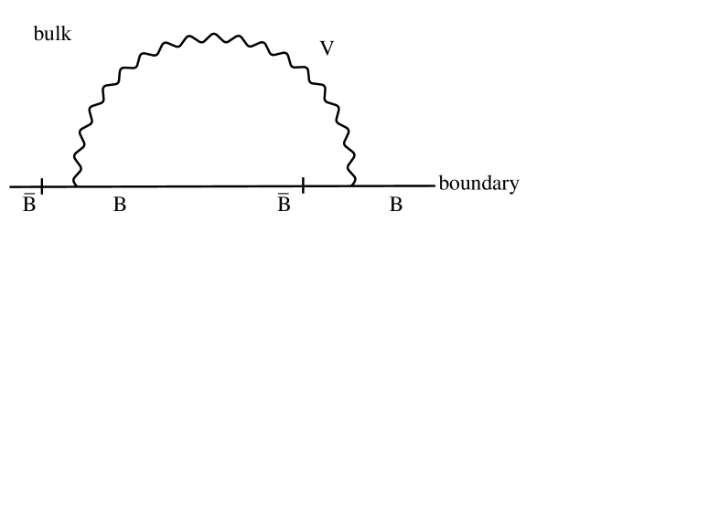
Figure 3: One loop contribution to the boundary propagator.

A standard one-loop calculation gives a contribution to the 1PI action. By virtue of Eqns. (B.1) and (B.3), we find

$$\Gamma^{\rm 1PI}_{B\bar{B}}=g^{2}\int\frac{d^{3}p}{(2\pi)^{3}}\frac{d^{3}k}{(2\pi)^{3}}\,d^{4}\theta\,B(\vec{p},\theta,\bar{\theta})\frac{-1}{2|\vec{p}+\vec{k}|}\frac{1}{\vec{k}^{2}}\bar{B}(\vec{p},\theta,\bar{\theta})\,$$ (B.10)

for the super-Feynman graph of Fig. 3. Since $\Gamma^{\rm 1PI}_{B\bar{B}}$ is logarithmically divergent, it follows that $\gamma_{B}\neq 0$ in general.

B.4 $\mathcal{N}=4$ model - Additional one loop correction to the boundary propagator for the defect field $B$

In addition to the expression (B.10), in the $\mathcal{N}=4$ model we find the following one-loop contribution to the 1PI action $\Gamma^{\rm 1PI}_{B\bar{B}}$, see Fig. 4:

Figure 4: One loop contribution to the boundary propagator.

$$\Gamma^{\rm 1PI}_{B\bar{B}}= \,g^{2}\int\frac{d^{3}p}{(2\pi)^{3}}\frac{d^{3}k}{(2\pi)^{3}}\,d^{4}\theta\,d^{4}\theta^{\prime}\,$$

$$\times B(-\vec{p},\theta,\bar{\theta})\left(-\frac{\bar{D}^{2}}{4}\right)\left(-\frac{D^{\prime}{}^{2}}{4}\right)\frac{\delta^{7}_{zz^{\prime}}}{2|\vec{p}+\vec{k}|}\frac{\delta^{7}_{zz^{\prime}}}{\vec{k}^{2}}\bar{B}(\vec{p},\theta,\bar{\theta})$$

$$= \,g^{2}\int\frac{d^{3}p}{(2\pi)^{3}}\frac{d^{3}k}{(2\pi)^{3}}\,d^{4}\theta\,B(\vec{p},\theta,\bar{\theta})\frac{1}{2|\vec{p}+\vec{k}|}\frac{1}{\vec{k}^{2}}\bar{B}(\vec{p},\theta,\bar{\theta})\,.$$ (B.11)

We see that this exactly cancels the contribution (B.10) such that $\gamma_{B}=0$ at least to one loop.

Appendix C The $\mathcal{N}=4$ model of (5.1) in $\mathcal{N}=1$, $d=3$ language

By construction, the model given by (5.1), (5.1) is the $\mathcal{N}=2$, $d=3$ formulation of the model constructed in [7] in $\mathcal{N}=1$, $d=3$ notation. To demonstrate this we note that the gauge field $V$ decomposes into [26]

$$V^{a}T^{a}\,=\,-i\,\Gamma^{\alpha a}\tilde{\theta}_{2\alpha}T^{a}\,+\,{\textstyle\frac{1}{2}}\,i\,\tilde{\theta}_{2}{}^{\alpha}\tilde{\theta}_{2\alpha}b^{a}T^{a}\,$$ (C.1)

under $\mathcal{N}=1$, $d=3$ supersymmetry. Here $\tilde{\theta}_{2}$ is defined in (2.2). The kinetic term in (5.1) decomposes into

$$\,\int\!d^{3}xd^{2}\tilde{\theta}_{1}\big{(}(\overline{\nabla q_{i}})\nabla q^{i}\,+bq^{i}\bar{q}_{i}\big{)}\,,\quad i=1,2\quad,$$ (C.2)

where the $\mathcal{N}=1$, $d=3$ superfield $q_{i}$ is defined as the lowest component in a $\tilde{\theta}_{2}$ expansion of $B_{i}$, $q_{i}=B_{i}|_{\tilde{\theta}_{2}=0}$. The covariant derivative in (C.2) is given by $\nabla\,=\,D-i\Gamma^{a}T^{a}$ with $D$ the $\mathcal{N}=1$, $d=3$ derivative. The kinetic term in (C.2) coincides with the boundary kinetic term given in (4.27) of [7] and $bq^{i}\bar{q}_{i}$ contributes to the superpotential term (4.29) of [7]. $b$ contains the auxiliary field $D$ defined in (2.21) above and thus $\partial_{2}{\rm Re}\phi^{\prime}$, which coincides with one of the three hypermultiplet scalar normal derivatives $D_{6}X_{H}{}^{A}$ which appear in the superpotential (4.29) of [7]. The superpotential term in (5.1) contains a complex auxiliary field $f$ and thus the two remaining hypermultiplet scalar derivatives of the form $D_{6}X_{H}{}^{A}$.

References

• [1] J.L. Cardy, Nucl. Phys. B 240 [FS12](1984) 514.
• [2] D.M. McAvity and H. Osborn, Nucl. Phys. B 455 (1995) 522, [arXiv:cond-mat/9505127];
D.M. McAvity and H. Osborn, Nucl. Phys. B 406 (1993) 655.
• [3] S. Sethi, Nucl. Phys. B 523, 158 (1998) [arXiv:hep-th/9710005].
• [4] O. J. Ganor and S. Sethi, JHEP 9801 (1998) 007 [arXiv:hep-th/9712071].
• [5] A. Kapustin and S. Sethi, Adv. Theor. Math. Phys.  2, 571 (1998) [arXiv:hep-th/9804027].
• [6] A. Karch and L. Randall, A. Karch and L. Randall, JHEP 0106 (2001) 063 [arXiv:hep-th/0105132].
• [7] O. DeWolfe, D.Z. Freedman and H. Ooguri, [arXiv:hep-th/0111135].
• [8] K. Hori, [arXiv:hep-th/0012179].
• [9] S. Sethi, private communication.
• [10] N. Arkani-Hamed, Th. Gregoire, J. Wacker, [arXiv:hep-th/0101233].
• [11] A. Hebecker, [arXiv:hep-ph/0112230].
• [12] A. Hanany and E. Witten, Nucl. Phys. B 492 (1997) 152. [arXiv:hep-th/9611230].
• [13] E. Ivanov, S. Krivonos and O. Lechtenfeld, Phys. Lett. B 487 (2000) 192 [arXiv:hep-th/0006017].
• [14] J.D. Lykken, [arXiv:hep-th/9612114].
• [15] H. Nishino and S.J. Gates, Int. J. Mod. Phys. A 8 (1993) 3371.
• [16] O. Aharony, A. Hanany, K. A. Intriligator, N. Seiberg and M. J. Strassler, Nucl. Phys. B 499 (1997) 67 [arXiv:hep-th/9703110].
• [17] T. E. Clark, O. Piguet and K. Sibold, Nucl. Phys. B 143 (1978) 445;
T. E. Clark, O. Piguet and K. Sibold, Nucl. Phys. B 172 (1980) 201;
T. E. Clark, O. Piguet and K. Sibold, Nucl. Phys. B 169 (1980) 77.
• [18] J. Erdmenger, C. Rupp and K. Sibold, Nucl. Phys. B 530 (1998) 501 [arXiv:hep-th/9804053];
J. Erdmenger and C. Rupp, Annals Phys.  276 (1999) 152 [arXiv:hep-th/9811209];
J. Erdmenger, C. Rupp and K. Sibold, Nucl. Phys. B 565 (2000) 363 [arXiv:hep-th/9907169].
• [19] O. Piguet and S. Sorella, Algebraic Renormalization. Springer Verlag, Berlin 1995;
J. Collins, Renormalization. Cambridge University Press 1984.
• [20] W. Zimmermann, Annals Phys.  77 (1973) 536 [Lect. Notes Phys.  558 (1973) 244];
T. E. Clark and J. H. Lowenstein, Nucl. Phys. B 113 (1976) 109.
• [21] N. Maggiore, O. Piguet and M. Ribordy, Helv. Phys. Acta 68 (1995) 264 [arXiv:hep-th/9504065]. O. M. Del Cima, D. H. Franco, J. A. Helayel-Neto and O. Piguet, JHEP 9802 (1998) 002 [arXiv:hep-th/9711191].
• [22] R. Brooks and S. J. Gates, Nucl. Phys. B 432 (1994) 205 [arXiv:hep-th/9407147].
• [23] A. Kapustin and M.J. Strassler, JHEP 9904 (1999) 021 [arXiv:hep-th/9902033].
• [24] B. M. Zupnik and D. V. Khetselius, Sov. J. Nucl. Phys.  47 (1988) 730 [Yad. Fiz.  47 (1988) 1147].
• [25] H. C. Kao, K. M. Lee and T. Lee, Phys. Lett. B 373 (1996) 94 [arXiv:hep-th/9506170].
• [26] E.A. Ivanov, Phys. Lett. B 268 (1991) 203.
• [27] L.V. Avdeev, D.I. Kazakov and I.N. Kondrashuk, Nucl. Phys. B 391 (1993) 333, [arXiv:hep-th/9302068].
• [28] P. C. Argyres, M. Ronen Plesser and N. Seiberg, Nucl. Phys. B 471 (1996) 159 [arXiv:hep-th/9603042].
• [29] P. West, “Introduction to supersymmetry and supergravity”, Second Edition, World Scientific Publishing, Singapore 1990.
• [30] S. Kachru and E. Silverstein, Phys. Rev. Lett.  80 (1998) 4855 [arXiv:hep-th/9802183].
• [31] E. Mirabelli and M. Peskin, Phys. Rev. D 58 (1998) 065002, [arXiv:hep-th/9712214].
• [32] H. Georgi, A.K. Grant and G. Hailu, Phys. Lett. B 506 (2001) 207, [arXiv:hep-ph/0012379].
• [33] S.J. Gates, M.T. Grisaru, M. Ro$\check{\rm c}$ek, and W. Siegel, Front. Phys. 58 (1983) 1, [arXiv:hep-th/0108200].