PUPT-1998

NEIP-01-009

LPTENS-02/11

hep-th/0202205

Recently, the author has proposed a generalization of the matrix and vector models approach to the theory of random surfaces and polymers. The idea is to replace the simple matrix or vector (path) integrals by gauge theory or non-linear $\sigma$ model (path) integrals. We explain how this solves one of the most fundamental limitation of the classic approach: we automatically obtain non-perturbative definitions in non-Borel summable cases. This is exemplified on the simplest possible examples involving ${\rm O}(N)$ symmetric non-linear $\sigma$ models with $N$-dimensional target spaces, for which we construct (multi)critical metrics. The non-perturbative definitions of the double scaled, manifestly positive, partition functions rely on remarkable identities involving (path) integrals.

February 2002

1 Motivations and example

Finding a general non-perturbative definition of string theory remains one of the most challenging problem in theoretical physics. One may hope that such a definition will automatically follow from an understanding of the basic principles of the theory and/or of quantum gravity, but for the moment we must rely on the ‘universal’ or ‘unique’ nature of the theory in order to gain an insight [1]. Historically, the first serious attempt at a non-perturbative approach was through the study of matrix models [2] and the double scaling limits [3]. The idea [4] was that near critical points, very large Feynman diagrams dominate, and thus in the ’t Hooft representation [5] the matrix theory reduces to a sum over continuous world-sheets. Comprehensive discussions of these subjects can be found in [6, 7, 8], and short introductions are in recent papers by the author [9, 10]. Unfortunately, the detailed investigations of the matrix integrals revealed that a non-perturbative definition of the most interesting theories, the unitary models which have non-Borel summable partition functions, could not be achieved. This point is discussed in details for example in Section 7 of [6]. Typically, the matrix model approach yields a differential equation, called the string equation, that determines unambiguously the perturbative, asymptotic series expansion, but that has several solutions differing by exponentially suppressed terms. For example, the string equation for the simplest critical point, that corresponds to pure two-dimensional gravity, is the Painlevé I differential equation [3]

$$z=u^{2}(z)+{1\over 3}u^{\prime\prime}(z)\,,$$ (1)

where the closed string coupling constant is $\kappa=z^{-5/4}$, and the connected partition function

$$W=\sum_{h=0}^{H}W_{h}\,\kappa^{2h-2}+{\cal O}(\kappa^{2H})$$ (2)

is such that $W^{\prime\prime}(z)=u(z)$. Equation (1) implies a recursion relation that determines all the coefficients $W_{h}$ once the sphere contribution $W_{0}$ is known. However, at large $h$, the coefficient $W_{h}$ goes like $(2h)!$, and thus the expansion (2) is not Borel summable and does not define a unique function. It turns out that solutions to (1) with the asymptotic expansion (2) are parametrized by an arbitrary real number, and differ at small $\kappa$ by terms of order $\exp(-4\sqrt{6}/(5\kappa))$ [3, 6, 8]. Those crucial non-perturbative contributions remain unknown. It is actually possible to understand in an elementary way why the matrix model fails to provide a non-perturbative definition. The model is defined by the integral over hermitian $N\times N$ matrices $M$,

$$\int\!d^{N^{2}}\!M\,\exp\Bigl{(}-{1\over 2}\mathop{\rm tr}\nolimits M^{2}-{g\over{N}}\mathop{\rm tr}\nolimits M^{4}\Bigr{)}\,,$$ (3)

and it turns out that the critical point lies at a negative value of $g$, for which the integral (3) is divergent. The same critical point could be obtained by starting from more general matrix integrals

$$\int\!d^{N^{2}}\!M\,\exp\Bigl{(}-{N\over g}\mathop{\rm tr}\nolimits U(M)\Bigr{)}\,,$$ (4)

with an arbitrary potential $U(M)$, but the fact is that the pure gravity, or any other unitary critical point, is always unstable. Shortly after the discoveries of [3], it was realized [11] that the same procedure could be applied to theories of polymers, by replacing matrix integrals like (4) by ${\rm O}(N)$ symmetric vector integrals like

$$\int\!d^{N}\vec{V}\,\exp\Bigl{(}-{N\over g}\,U({\vec{V}}^{2})\Bigr{)}\,.$$ (5)

In addition to their intrinsic interest, the polymer integrals are useful toy models for the more complicated string theories. An interesting aspect is that higher dimensional vector path integrals can be easily studied [12], in contrast to the matrix case. Works on the vector models are reviewed in [13]. However, the basic problem stressed above, that non-perturbative results cannot be obtained in the most interesting non-Borel summable cases, plagues the vector integrals in the same way as it plagues the matrix integrals, and for the same reasons. In spite of several attempts over the years (see in particular [14] and references therein), this fundamental drawback of the matrix (or vector) models approach could never be satisfactorily solved. However, very recenty, the author made a simple proposal that automatically overcome the difficulty [15, 16, 9, 10]. The purpose of the present note is to show explicitly how this proposal works in the simplest possible examples.

The idea is to replace the simple matrix (4) or vector (5) (path) integrals by some gauge theory or non-linear $\sigma$ models (path) integrals respectively. The non-trivial result is that analogues of the Kazakov critical points [4] exist in those cases as well. For two dimensional non-linear $\sigma$ models, it was shown in [15] that mass terms for the would-be Goldstone bosons could be adjusted to critical values, and double scaling limits defined. It was also argued at length in [15] that mass (or more generally potential) terms in non-linear $\sigma$ models are very similar to Higgs vevs in gauge theories. And indeed in [16, 9] is was shown that in four dimensional supersymmetric gauge theories, the adjoint Higgs vevs moduli can also be adjusted to critical values and double scaling limits defined, with the Argyres-Douglas singularities [17] playing the rôle of the Kazakov critical points. This yields four dimensional non-critical (or five dimensional critical) string theories [9]. In all those examples, the double scaling limits are always non-perturbative, because the original integrals are convergent for all values of the parameters.

To illustrate this point, we will focus in the following on $D=0$, $1$ or $2$ dimensional non-linear $\sigma$ model examples, akin to the model studied in [15]. In those cases, the large $N$ expansion is a loop expansion in the dual representation of Feynman diagrams and, as reviewed in [10], this implies that the double scaled theories are field theories themselves (in contrast with the gauge theory case which yields string theories). In spite of this considerable simplification, the basic difficulty remains the same. For example, the simplest non-Borel summable double scaled field theoretic partition function we will encounter is

$$e^{W(\kappa)}=Z(\kappa)=\int\!{dx\over\sqrt{2\pi}}\,e^{-x^{2}/2+\kappa x^{4}/4}.$$ (6)

Obviously, this integral diverges, but admits a well-defined perturbative expansion

$$Z(\kappa)=1+\sum_{k=1}^{K}{(4k-1)!\over 2^{4k-1}k!(2k-1)!}\,\kappa^{k}+{\cal O}(\kappa^{K+1}).$$ (7)

The integral representation (6) makes ‘unitarity’ obvious: each diagram will have a positive weight. This has the usual consequence that all the coefficients in the series expansion for $W=\ln Z$ are positive, and the series is not Borel summable. The ‘string equation,’ analogue to (1), is the Schwinger-Dyson equation for (6). It takes a simple form when written in terms of $Z$,

$$16\kappa^{2}\,Z^{\prime\prime}+4(8\kappa-1)\,Z^{\prime}+3\,Z=0\,.$$ (8)

With the condition $Z=1+{\cal O}(\kappa)$, this equation implies the asymptotic expansion (7), in the same way as (1) implies a unique expansion (2). And also in strict parallel with (1), there is a one parameter family of solution to (8) with the correct asymptotic behaviour. It can be written in terms of modified Bessel functions,

$$Z_{\theta}(\kappa)={\sqrt{\pi}e^{-1/(8\kappa)}\over 4\sqrt{\kappa}}\left[I_{1/4}\Bigl{(}{1\over 8\kappa}\Bigr{)}+I_{-1/4}\Bigl{(}{1\over 8\kappa}\Bigr{)}+\theta\Bigl{[}I_{1/4}\Bigl{(}{1\over 8\kappa}\Bigr{)}-I_{-1/4}\Bigl{(}{1\over 8\kappa}\Bigr{)}\Bigr{]}\right].$$ (9)

The combination $I_{1/4}-I_{-1/4}$ is a purely non-perturbative contribution to $Z$. In agreement with the high order behaviour of (7), it yields terms proportional to $\exp(-1/(4\kappa))$ that remain unknown.

In the standard matrix case [6], equations (1) and (2), we have no hint to the value of the $\theta$ parameter. It is actually far from being obvious that there exists a ‘correct’ solution to (1), in the sense that it corresponds to a well-defined non-perturbative string theory. It is not even known how to make this statement precise. On the other hand, in the case of equations (8) and (7), the problem can be formulated easily, because a non-perturbatively defined zero-dimensional field theory is simply characterized by a potential which is bounded from below. This means that ‘correct’ values of $\theta$ should be such that there exists $V_{\kappa,\theta}$ for which

$$Z_{\theta}(\kappa)=\int\!{dx\over\sqrt{2\pi}}\,e^{-x^{2}/2-V_{\kappa,\theta}(x)}.$$ (10)

We have not tried to solve directly (10) for $\theta$ and $V_{\kappa,\theta}$, but we will see that the non-linear $\sigma$ model approach yields unambiguously the potential

$$V_{\kappa}(x)=\ln 2+\sqrt{\kappa/8}\,x^{3}+\kappa x^{4}/16$$ (11)

which corresponds to $\theta=0$. The $\ln 2$ term takes care of the two equivalent minima of $V_{\kappa}$ that occur at $x=0$ and $x=-2\sqrt{2/\kappa}$. The fact that (11) is a solution relies on the nice identity

$$\langle e^{-\sqrt{\kappa/8}\,x^{3}-\kappa x^{4}/16}\rangle_{\rm pert}=\langle e^{\kappa x^{4}/4}\rangle_{\rm pert}\,,$$ (12)

where $\langle\cdots\rangle_{\rm pert}$ is the perturbative expansion in $\kappa$ with $\langle x^{2}\rangle_{\rm pert}=1$. Remarkably, we will see in Section 3 that (12) can be generalized to the case of path integrals.

We have not proven that $\theta=0$ with the potential (11) is the only solution to (10), but we believe that this is likely to be the case, because identities like (12) are very peculiar. This illustrates the point [9, 10] that the gauge theory or non-linear $\sigma$ model integrals we start from yield the correct and probably unique non-perturbative definitions of the double scaled theories. This is an important point of principle, because even though the general arguments [5, 4] show that double scaled matrix integrals reproduce the perturbative expansion of string theories, there might be a priori a distinction between non-perturbative string theory and non-perturbative matrix integral.

2 Simple integrals

We will consider the most general ${\rm O}(N)$ symmetric non-linear $\sigma$ model with a compact target space $\cal M$ of dimension $N$ and quadratic mass terms. By using cartesian coordinates $(x_{1},\ldots,x_{N},x_{N+1}=z)$, the equation for the target space can be written in terms of a single function $f(z)$ as

$${\cal M}:\ \sum_{i=1}^{N}x_{i}^{2}={\vec{x}}^{2}=f(z)\,.$$ (13)

We will limit our investigations to the cases where $f(z)$ is a polynomial. At the North pole $z=z_{N}>0$ we have $f(z_{N})=0$ and $f^{\prime}(z_{N})<0$. We will see below that for theories with critical points, there exists a $z<z_{N}$ for which $f^{\prime}$ vanishes. We will choose the coordinates $\vec{x}$ and $z$ such that

$$f(0)=1\,,\quad f^{\prime}(0)=0\,,\quad f^{\prime}(z)<0\ {\rm for}\ z\in]0,z_{N}]\,.$$ (14)

The metric can be written in terms of the local inverse $F=f^{-1}$ of $f$ as

$$g=\left(\delta_{ij}+4F^{\prime}({\vec{x}}^{2})^{2}x_{i}x_{j}\right)\,dx_{i}\otimes dx_{j}\,,$$ (15)

and the partition function is

$${\cal Z}=\int_{\cal M}\!{d^{N}\vec{x}\,\sqrt{\det g}\over{\rm Vol}({\cal M})}\,e^{-Nr{\vec{x}}^{2}/2}\,,$$ (16)

where $r$ is the mass parameter and ${\rm Vol}({\cal M})$ the volume of $\cal M$. The large $N$ limit will be taken at fixed $r$. By rescaling the coordinates, we see that taking the large $r$ limit is equivalent to taking the large target space, or weak coupling, limit. The coupling constant for the theory is thus $1/r$. Equivalently, we can say that our models are asymptotically free, and the large mass limit corresponds to a weak coupling limit.

2.1 Sphere

Let us start with the simplest case corresponding to ${\cal M}=S^{N}$ and

$$f(z)=1-z^{2}\,.$$ (17)

The first question one may ask is whether a proper ‘polymer’ interpretation of the theory can be given. This is not obvious, because the contribution of the metric in (16), which in the case of the sphere is $\sqrt{\det g}=1/\sqrt{1-{\vec{x}}^{2}}$, does not scale properly. However, this is due to a bad choice of coordinates, and it is possible to cast (16) in the form (5). To do that, we first introduce the spherical angle $\theta$, in terms of which

$${\cal Z}={\Gamma((N+1)/2)\over\sqrt{\pi}\,\Gamma(N/2)}\int_{0}^{\pi}\!d\theta\,(\sin\theta)^{N-1}e^{-{Nr\over 2}\sin^{2}\theta}\,.$$ (18)

We then interpret $\theta$ as a radial coordinate emanating from the North (or South) pole for an $N$-dimensional plane $(V_{1},\ldots,V_{N})$, $\theta=|\vec{V}|/\sqrt{r}=\rho/\sqrt{r}$. Physically, this plane approximate the sphere for large $r$, and we can expect that the effects of the deviation from the sphere can be taken into account in an effective potential. Indeed, the partition function (18) can be rewritten as

$${\cal Z}={\Gamma((N+1)/2)\over 2\pi^{(N+1)/2}r^{N/2}}\int_{|\vec{V}|\leq\pi\sqrt{r}}\!d^{N}\vec{V}\,e^{-NU_{N}({\vec{V}}^{2})}$$ (19)

with

$$U_{N}(\rho^{2})={r\over 2}\sin^{2}(\rho/\sqrt{r})-{N-1\over N}\ln{\sqrt{r}\sin(\rho/\sqrt{r})\over\rho}\,\cdotp$$ (20)

One can then show straightforwardly that for the purposes of the double scaling limits, which involve the $N\rightarrow\infty$ limit, we can use the $N$-independent potential

$$U(\rho^{2})={r\over 2}\sin^{2}(\rho/\sqrt{r})-\ln{\sqrt{r}\sin(\rho/\sqrt{r})\over\rho}$$ (21)

and the integral

$$\int_{|\vec{V}|\leq\pi\sqrt{r}}\!d^{N}\vec{V}\,e^{-NU({\vec{V}}^{2})}\,.$$ (22)

We thus get a standard Feynman diagram interpretation, because the constraint $|\vec{V}|\leq\pi\sqrt{r}$ cannot be seen in perturbation theory. We could then keep using (22) and study the critical point and double scaling limit. However, we prefer to present alternative derivations using (16) or (18).

The integral (18) can be explicitly calculated, by expanding $\exp(-(Nr/2)\sin^{2}\theta)$ in power series and performing the integrals using Euler $B$ function. This yields a series for a confluent hypergeometric function, and we get

$${\cal Z}={}_{1}F_{1}(N/2,(N+1)/2;-Nr/2)=e^{-Nr/2}{}_{1}F_{1}(1/2,(N+1)/2;Nr/2)\,.$$ (23)

The first expression is useful to obtain the asymptotic expansion at large $r$,

$${\cal Z}={\Gamma((N+1)/2)\over\sqrt{\pi}(Nr)^{N/2}}\left[\sum_{k=1}^{K}{\Gamma(N/2+k)\Gamma(k+1/2)\over\sqrt{\pi}\,\Gamma(N/2)k!}\Bigl{(}{2\over rN}\Bigr{)}^{k}+{\cal O}(1/r^{K+1})\right]\,,$$ (24)

while the second expression yields a convergent strong coupling expansion

$${\cal Z}={\Gamma((N+1)/2)\over\sqrt{\pi}}\sum_{k=0}^{\infty}{\Gamma(k+1/2)\over k!\,\Gamma(k+(N+1)/2)}\Bigl{(}{rN\over 2}\Bigr{)}^{k}\,.$$ (25)

The large $N$ expansion can be obtained as usual from the perturbative expansion (24) by resumming the contributions at each order in $1/N$. It is convenient to introduce a rescaled partition function

$$\tilde{\cal Z}=\sqrt{1-1/r}\,{\sqrt{\pi}(Nr/2)^{N/2}\over\Gamma((N+1)/2)}\,{\cal Z}\,,$$ (26)

for which we have when $r>1$

$$\tilde{\cal Z}=1+{3\over 4(r-1)^{2}N}+\Bigl{(}{5\over 2(r-1)^{3}}+{105\over 32(r-1)^{4}}\Bigr{)}{1\over N^{2}}+{\cal O}(1/N^{3})\,.$$ (27)

We see that the $1/N$ expansion breaks down when $r\rightarrow 1^{+}$. At $r=1$ we have a Kazakov critical point, and (27) suggests to consider the double scaling limit

$$N\rightarrow\infty\,,\quad r\rightarrow 1^{+}\,,\quad N(r-1)^{2}=1/\kappa={\rm constant}.$$ (28)

In such a limit, only the most singular, universal, terms in (27) survive, and we get

$$\tilde{\cal Z}\rightarrow Z=1+{3\over 4}\,\kappa+{105\over 32}\,\kappa^{2}+{\cal O}(\kappa^{3})\,.$$ (29)

To show that the scaling (28) is consistent to all orders, one can use directly (23) and check that the corresponding hypergeometric differential equation reduces to the ‘string equation’ (8). However, this method does not yield the value of $\theta$ in (9). The most fruitful approach, that can be generalized to the case of path integrals (see for example [15, 16]), is to implement the constraint (13) with a Lagrange multiplier $\alpha$ and then perform explicitly the integral over $\vec{x}$. We obtain

$${\cal Z}\propto\int_{-\infty}^{+\infty}\!dzd\alpha\,e^{-Nv_{\rm eff}(z,\alpha)}\,,$$ (30)

with the effective potential

$$v_{\rm eff}(z,\alpha)={1\over 2}(r-\alpha)f(z)+{1\over 2}\ln\alpha\,.$$ (31)

We are not keeping track of the trivial prefactors, because they can be restored easily on the double scaled partition functions by using the normalization condition $Z=1+{\cal O}(\kappa)$. At large $N$, $\cal Z$ is dominated by the minima of $v_{\rm eff}$. It is straightforward to check that for $r>1$ (weak coupling) the stable saddle points are

$$z_{*}=\pm\sqrt{1-1/r}\,,\quad\alpha_{*}=r\,,$$ (32)

while for $r<1$ (strong coupling) we have

$$z_{*}=0\,,\quad\alpha_{*}=1\,.$$ (33)

We recover the critical point at $r=1$, where a transition corresponding to the merging of the two weakly coupled saddle points occurs. Since we are interested in the vicinity of the critical point only, and the critical variable is $z$, we can integrate over $\alpha$ by using the equation $\partial v_{\rm eff}/\partial\alpha=0$ which yields $\alpha=1/f(z)$. By rescaling $z\rightarrow z/N^{1/4}$ and expanding the potential (31) around $z=0$, we get

$${\cal Z}\propto\int_{-\infty}^{+\infty}\!dz\,e^{\sqrt{N}(r-1)z^{2}/2-z^{4}/4+{\cal O}(1/\sqrt{N})}\,.$$ (34)

We then immediately see that the scaling (28) yields

$$Z(\kappa)={e^{-1/(4\kappa)}\over\sqrt{4\pi}}\int_{-\infty}^{+\infty}\!dx\,e^{x^{2}/2-\kappa x^{4}/4}\,,$$ (35)

where we have used the variable $x=\kappa^{1/4}z$ and we have restored the prefactors. The formula (10) with the potential (11) is obtained by substituting $x\rightarrow 1/\sqrt{\kappa}+\sqrt{2}\,x$.

As opposed to the case of ordinary vector or matrix models, our partition function is perfectly well-defined at strong coupling and we can go through the critical point at $r=1$. Equation (34) is actually valid both for $r>1$ and for $r<1$, and it shows that we can consider a double scaling limit from strong coupling,

$$N\rightarrow\infty\,,\quad r\rightarrow 1^{-}\,,\quad N(r-1)^{2}=1/\kappa={\rm constant}\,,$$ (36)

yielding a “dual” double scaled partition function

$$Z_{\rm D}(\kappa)=\int_{-\infty}^{+\infty}\!{dx\over\sqrt{2\pi}}e^{-x^{2}/2-\kappa x^{4}/4}\,.$$ (37)

Of course, $\cal Z$ does not have a Feynman diagram expansion for $r<1$ and thus $Z_{\rm D}$ does not have an interpretation in terms of ‘polymers.’ However, the very existence of $Z_{\rm D}$, which relies on the fact that our non-linear $\sigma$ model is non-perturbatively defined, has some interesting consequences. The common origin (34) of the weak-coupling (35) and strong coupling (37) partition functions implies that $\int\exp(x^{2}/2-\kappa x^{4}/4)dx$ and $\int\exp(-x^{2}/2-\kappa x^{4}/4)dx$ satisfy the same ‘string’ equation

$$16\kappa^{2}\,y^{\prime\prime}+4(8\kappa+1)\,y^{\prime}+3\,y=0\,.$$ (38)

The Borel summable, alternate series solution of (38) yields $Z_{\rm D}$ while the non-Borel summable solution yields $\exp(1/(4\kappa))\,Z$. $Z$ itself actually satisfies (38) with $\kappa\rightarrow-\kappa$, see (8), and thus the equation (37) immediately implies the identity (12).

2.2 Multicritical metrics

Let us now study the case of a general metric (15). Equation (30) is replaced by

$${\cal Z}\propto\int_{-\infty}^{+\infty}\!dzd\alpha\,e^{-Nv_{\rm eff}(z,\alpha)+{1\over 2}\ln(4f(z)+f^{\prime}(z)^{2})}\,,$$ (39)

with the potential (31). The saddle point equations read

$$\alpha=1/f(z)\,,\quad(r-\alpha)f^{\prime}(z)=0\,.$$ (40)

The analysis is then very similar to the case of the sphere, equations (32) and (33). At weak coupling, the stable saddle point is

$$z_{*}=f^{-1}(1/r)=F(1/r)\,,\quad\alpha_{*}=r\,.$$ (41)

This is valid as long as $r>1$. Because on the conditions on $f$ listed in (14), a critical point occurs at $r=1$ and the stable saddle point for $r<1$ is given by (33). The critical variable being $z$, we can integrate out $\alpha$ for the purposes of the double scaling limits. The term $\ln(4f+f^{\prime 2})$ is also irrelevant in these limits. We can thus work with

$$\int_{-\infty}^{+\infty}\!dz\,e^{-Nv(z;r)}\,,$$ (42)

where the potential is

$$v(z;r)={r\over 2}f(z)-{1\over 2}\ln f(z)\,.$$ (43)

We have $v(z;r=1)=v(0,r=1)+{\cal O}(z^{p})$. It turns out that only even values of $p\geq 4$ can be obtained. The $m^{\rm th}$-critical point, $m\geq 2$, is defined by the condition $v(z;r=1)=v(0;r=1)+{\cal O}(z^{2m})$. It corresponds to the choice

$$f_{m}(z)=1-a_{m}z^{m}\,,$$ (44)

where $a_{m}$ is an arbitrary positive real number. Relevant deformations are defined to be the perturbations of $f_{m}$ that generate terms of order $z^{k}$ for $k\leq 2m-1$ in the potential $v$. A priori one may want to consider

$$f(z)=f_{m}(z)-z^{2}\sum_{k=0}^{2m-3}\epsilon_{k}z^{k}\,,$$ (45)

but it is easily checked that only the $\epsilon_{k}$ for $0\leq k\leq m-3$ can survive in a consistent double scaling limit. Together with $\delta=r-1$, we thus have $m-1$ relevant operators at the $m^{\rm th}$ order critical point. The correct scaling is

$$N\rightarrow\infty\,,\quad N\delta^{2}={\rm cst}=1/\kappa\,,\quad N^{{m-k-2\over 2m}}\epsilon_{k}={\rm cst}\propto t_{k}\,.$$ (46)

With a suitable normalization for the $t_{k}$s, and by defining $t_{m-2}=1$, the $m^{\rm th}$ order double scaled partition function can then be written as

$$Z_{m}\propto\int_{-\infty}^{+\infty}\!dx\,\exp\Bigl{(}\sum_{k=0}^{m-2}t_{k}\,x^{k+2}-\kappa\sum_{k=0}^{2m-4}\!\!\!\sum_{\scriptstyle k_{1}+k_{2}=k\atop\scriptstyle 0\leq k_{1},k_{2}\leq m-2}\!\!\!\!t_{k_{1}}t_{k_{2}}\,x^{k+4}\Bigr{)}\,.$$ (47)

The ‘coupling constant’ $\kappa$ could of course be absorbed in the definition of the $t_{k}$s. It is singled out by the fact that it is the most relevant deformation, as the scaling (46) shows. For $m=2$, we recover (35), while for higher criticality we obtain, for example,

$$Z_{3}\propto\int_{-\infty}^{+\infty}\!dx\,e^{t_{0}x^{2}+x^{3}-\kappa(t_{0}^{2}x^{4}+2t_{0}x^{5}+x^{6})}\,,$$ (48)

$$Z_{4}\propto\int_{-\infty}^{+\infty}\!dx\,e^{t_{0}x^{2}+t_{1}x^{3}+x^{4}-\kappa(t_{0}^{2}x^{4}+2t_{0}t_{1}x^{5}+(t_{1}^{2}+2t_{0})x^{6}+2t_{1}x^{7}+x^{8})}\,,\quad{\rm etc\ldots}$$ (49)

From (47), all correlators can of course be calculated, by taking derivatives with respect to the parameters. One can also study positivity by looking at the partition functions when only $\kappa$ is turned on. The formula generalizing (35) is

$$Z_{m}(\kappa)={me^{-1/(4\kappa)}\over 2^{(1+(-1)^{m})/2}\sqrt{2\pi}(2\kappa)^{1/2-1/m}}\int_{-\infty}^{+\infty}\!dx\,e^{x^{m}-\kappa x^{2m}}\,,$$ (50)

where the normalization is chosen such that $Z_{m}=1+{\cal O}(\kappa)$. The ‘string equation’ is

$$4m\kappa^{2}\,Z^{\prime\prime}_{m}+\left(2(5m-2)\kappa-m\right)\,Z^{\prime}_{m}+{(2m-1)(m-1)\over m}\,Z_{m}=0\,,$$ (51)

from which one can deduce the perturbative expansion of $Z_{m}$, for which all the coefficients are positive. The same is true for $\ln Z_{m}$, as required by a correct statistical polymer interpretation. This is manifest from equation (12) in the case $m=2$, and can be proven for general $m$ from the differential equation. Finally, let us note that it is possible to evaluate explicitly the integrals (50). The idea is to perform a strong coupling expansion at large $\kappa$. From experience, we know that such expansions are often convergent. The expansion is obtained by rescaling $x^{2m}\rightarrow x^{2m}/\kappa$ in (50) and expanding the exponential in powers of $1/\sqrt{\kappa}$. The resulting integrals are elementary, and the final result is a hypergeometric series. We end up with

$$Z_{m}(\kappa)={\Gamma(1/(2m))\,e^{-1/(4\kappa)}\over 2^{1-1/m+(-1)^{m}/2}\sqrt{2\pi}\kappa^{1/2-1/(2m)}}\,{}_{1}F_{1}(1/(2m),1/2;1/(4\kappa))$$ (52)

for $m$ odd and

$$\hskip-42.67912ptZ_{m}(\kappa)={e^{-1/(4\kappa)}\over 2^{1-1/m+(-1)^{m}/2}\sqrt{2\pi}\kappa^{1/2-1/(2m)}}\,\Bigl{(}\Gamma(1/(2m))\,{}_{1}F_{1}(1/(2m),1/2;1/(4\kappa))$$

$$\hskip 99.58464pt+{\Gamma(1/2+1/(2m))\over\sqrt{\kappa}}\,{}_{1}F_{1}(1/2+1/(2m),3/2;1/(4\kappa))\Bigr{)}$$ (53)

for $m$ even. In the special case $m=2$, there is a relation between the confluent hypergeometric functions appearing in (53) and the Bessel functions, and we recover (9) with $\theta=0$.

3 Path integrals

The results of the previous Section can be generalized to the case of path integrals. For the sake of brevity, we will consider only the lower critical point corresponding to a sphere target space. In one dimension, the resulting model is the quantum version of a famous integrable mechanical problem first studied by C. Neumann [18]: the motion of a particle of mass $m$ on the $N$ dimensional sphere of radius $a$, with a quadratic potential characterized by the pulsation $\omega$. Quantum mechanically, there are two regimes. When the sphere is very large, the effects of the curvature are negligible, and the problem is well approximated by the $N$ dimensional harmonic oscillator. This weakly coupled regime is valid as long as the harmonic oscillator wave functions extend on a distance much smaller that $a$, that is

$$r={m\omega a^{2}\over N\hbar}\gg 1\,.$$ (54)

On the other hand, when $r\ll 1$, the hamiltonian reduces to the exactly solvable rigid rotator, around which a strong coupling expansion can be performed. At the transition between these two qualitatively different regimes lies the critical point we will use to define the double scaling limit. In suitable units, the euclidean partition function that generalizes (16) is

$${\cal Z}_{T}=\int\!\left[d^{N}\vec{x}(t)\,\sqrt{\det g(\vec{x}(t))}\right]\,\exp\left[-{Nr\over 2}\int_{-T/2}^{T/2}\!dt\Bigl{(}g_{ij}\,{dx^{i}\over dt}{dx^{j}\over dt}+{\vec{x}}^{2}\Bigr{)}\right]\,,$$ (55)

where the path integral measure is normalized such that the ground state energy $E$ for the hamiltonian

$$H={{\vec{L}}^{2}\over 2N^{2}}+{r^{2}\over 2}{\vec{x}}^{2}\,,$$ (56)

where $-{\vec{L}}^{2}$ is the Laplacian on the $N$-sphere, is given by

$$E=-{r\over N}\lim_{T\rightarrow\infty}{\ln{\cal Z}_{T}\over T}\,\cdotp$$ (57)

It is interesting to note that, as in the case of the zero-dimensional integrals (equations (19) and (20)), the perturbation theory in $1/r$ for the quantum mechanical non-linear $\sigma$ model (55) is reproduced by a linear $\sigma$ model with a suitable potential that encodes the effects of the curvature of the sphere. By using the coordinates $\vec{V}$ defined at the beginning of Section 2.1, and by rescaling the wave functions $\psi\rightarrow\psi/(\sin\theta)^{(N-1)/2}$, the Schrödinger equation for the ground state of (56) can indeed be cast in the form

$$-{1\over 2N^{2}}\,\Delta\psi+U_{N}(|\vec{V}|)\,\psi={E\over r}\,\psi\,,$$ (58)

where now $\Delta$ is the flat $N$-dimensional Laplacian and

$$U_{N}(\rho)=-{N-1\over 4rN^{2}}+{(N-3)(N-1)\over 8N^{2}}\Bigl{(}{1\over r\tan^{2}(\rho/\sqrt{r})}-{1\over\rho}\Bigr{)}+{r\over 2}\sin^{2}(\rho/\sqrt{r})\,.$$ (59)

As a side remark, let us note that the formulation given by the equations (58) and (59), in addition to providing a consistent polymer interpretation in the double scaling limit, allows one to evaluate, using standard linear $\sigma$ model techniques, the large order behaviour of perturbation theory for a non-linear $\sigma$ model. As we will see later, the perturbation series is not Borel summable. From the linear $\sigma$ model point of view, the non-perturbative contributions depend on the boundary conditions at $\rho=\pi\sqrt{r}$ that must be imposed to recover the full non-linear model. This is particularly obvious in the case $N=1$, which can be solved exactly in terms of Mathieu functions. In general, by taking into account the exponential decrease of the harmonic oscillator wave functions, we see that the non-perturbative contributions are of order $\exp(-N\pi^{2}r/2)$, which is an instanton effect from the non-linear $\sigma$ model point of view.

Equation (58) shows that the large $N$ limit is a semi-classical limit, since $N^{2}$ plays the rôle of $\hbar$. We could use this idea to study the $1/N$ expansion. However, it is more convenient to use the Lagrange multiplier method, as in the case of the zero dimensional integrals (30). We obtain

$${\cal Z}\propto\int\!\left[dz(t)d\alpha(t)\right]\,e^{-Ns_{\rm eff}[z,\alpha]}\,,$$ (60)

with the effective action

$$s_{\rm eff}[z,\alpha]={r\over 2}\int\!dt\,\Bigl{[}\Bigl{(}{dz\over dt}\Bigr{)}^{2}+(\alpha-1)z^{2}-\alpha\Bigr{]}+{1\over 2}\mathop{\rm tr}\nolimits\ln\Bigl{(}-{d^{2}\over dt^{2}}+\alpha\Bigr{)}\,.$$ (61)

The saddle points can be deduced from the effective potential which is derived from (61) by taking $\alpha$ constant,

$$v_{\rm eff}={r\over 2}\Bigl{[}(\alpha-1)z^{2}-\alpha\Bigr{]}+{\sqrt{\alpha}\over 2}\,\cdotp$$ (62)

For $r>1/2$ (weak coupling) we get

$$z_{*}=\pm\sqrt{1-1/(2r)}\,,\quad\alpha_{*}=1\,,$$ (63)

while for $r<1/2$ (strong coupling) we have

$$z_{*}=0\,,\quad\alpha_{*}=1/(4r^{2})\,.$$ (64)

The critical point occurs at $r=1/2$. To perform explicitly the double scaling limit, we introduce the rescaled variables

$$\tau=N^{-1/3}t\,,\quad x=N^{1/3}z\,,\quad\beta=N^{2/3}(\alpha-1)\,,\quad\kappa^{-1}=N(r-1/2)^{3/2}\,,$$ (65)

in terms of which

$$Ns_{\rm eff}={1\over 4}\int\!d\tau\,\Biggl{[}\Bigl{(}{dx\over d\tau}\Bigr{)}^{2}+\beta(x^{2}-2\kappa^{-2/3})-{\beta^{2}\over 4}\Biggr{]}+{\cal O}(1/N^{2/3})\,.$$ (66)

Rescaling $\tau\rightarrow\kappa^{1/3}\tau/\sqrt{2}$ and $x\rightarrow 2^{1/4}\kappa^{1/6}x$, we see that the double scaling limit

$$N\rightarrow\infty\,,\quad r\rightarrow 1/2^{+}\,,\quad N(r-1/2)^{3/2}=1/\kappa={\rm constant}$$ (67)

yields the double scaled partition function

$$Z(\kappa)=\int\![dx(t)]\,\exp\left[-\int\!d\tau\,\Biggl{(}{1\over 2}\Bigl{(}{dx\over d\tau}\Bigr{)}^{2}-x^{2}+{\kappa x^{4}\over 2\sqrt{2}}+{1\over\sqrt{2}\kappa}\Biggr{)}\right]\,,$$ (68)

where we have integrated out the auxiliary field $\beta$ and the $\kappa$-independent measure $[dx]$ is normalized such that $Z=1+{\cal O}(\kappa)$ as usual. Equation (68) is the one-dimensional version of equation (35).

There remains to check our main point, that the perturbative expansion of (68), or more precisely of $W=\ln Z$, has only positive coefficients and is not Borel summable. The perturbative series is obtained by expanding around the two equivalent minima of the potential $V(x)=-x^{2}+\kappa x^{4}/(2\sqrt{2})$. After a shift of the variable $x$, we obtain the one-dimensional version of (10) and (11),

$$Z(\kappa)=\int\![dx(t)]\,\exp\left[-\int\!d\tau\,\Biggl{(}{1\over 2}\Bigl{(}{dx\over d\tau}\Bigr{)}^{2}+2x^{2}\Bigl{(}1-{\sqrt{\kappa}\over 2^{5/4}}x\Bigr{)}^{2}\Biggr{)}\right]\,.$$ (69)

In zero dimensions, positivity was obvious thank’s to the identity (12). Remarkably, a similar and highly non-trivial identity exists in one dimension as well [19]. It reads

$$Z(\kappa)\,\mathop{=}_{\rm pert}\,\Bigl{\langle}\exp\Bigl{(}{\kappa\over 2^{7/2}}\int\!d\tau\,|z|^{4}\Bigr{)}\Bigr{\rangle}_{\rm pert}\,,$$ (70)

where $z=z_{1}+iz_{2}$ is a complex coordinate, and the average $\langle\cdots\rangle_{\rm pert}$ is defined by the canonically normalized propagator $\langle z_{i}(\tau)z_{j}(0)\rangle_{\rm pert}=e^{-|\tau|}\,\delta_{ij}/2$. The equality is valid to all orders of perturbation theory. The left hand side can be viewed as giving the probably unique field theoretic non-perturbative definition of the manifestly positive and non Borel summable partition function on the right hand side.

One could go further and study multicritical metrics as in Section 2. We will let this exercise to the reader, and rather close this paper with a two dimensional example. The partition function we start from, that replaces (16) and (55), is

$${\cal Z}=\int\!\left[d^{N}\vec{x}(\sigma)\,\sqrt{\det g(\vec{x}(\sigma))}\right]\,\exp\left[-{N\over 2g^{2}}\int\!d^{2}\sigma\Bigl{(}g_{ij}\,\partial_{a}x^{i}\partial_{a}x^{j}+m^{2}{\vec{x}}^{2}\Bigr{)}\right]\,.$$ (71)

The theory needs to be renormalized, and quantum mechanically the dimensionless coupling $g$ is replaced by a mass scale $\Lambda$. The only dimensionless parameter is then $r=m^{2}/\Lambda^{2}$. One can give straightforwardly a ‘polymer’ interpretation to (71), by using dimensional regularization, because in that case the non-trivial factor in the path integral measure drops out, and the other terms have automatically the correct ’t Hooft scaling. This is unlike the $D=0$ or $D=1$ cases discussed previously, for which a reformulation in terms of a linear $\sigma$ model was needed. One can then show that there is a critical point at $r=1$, and that in the double scaling limit

$$N\rightarrow\infty\,,\ \delta=r-1\rightarrow 0^{+}\,,\ N\delta-3\ln N={\rm constant}={1\over 2\kappa}+3\ln\kappa\,,\ \sigma^{a}=\sqrt{N}\,x^{a}\,,$$ (72)

the partition function reduces to

$$Z(\kappa)=\int\![d\phi(x)]\,\exp\Biggl{[}-\int\!d^{2}x\,\Bigl{(}{1\over 2}\,\partial_{a}\phi\partial_{a}\phi-{\Lambda^{2}\over 4\kappa}:\!\phi^{2}\!:+\pi\Lambda^{2}:\!\phi^{4}\!:\Bigr{)}\Biggr{]}\,.$$ (73)

The proof can be found in [15]. The $\ln N$ correction to the naïve scaling in (72) is reminiscent of the $c=1$ matrix model [20]. The normal ordering is defined at the scale $\mu=\Lambda/\sqrt{\kappa}$ so that there is no tadpole in perturbation theory. The perturbative expansion is indeed obtained after shifting the field $\phi\rightarrow 1/\sqrt{8\pi\kappa}+\phi$ and writing (73) in the form

$$Z(\kappa)=\int\![d\phi(x)]\,\exp\Biggl{[}-\int\!d^{2}x\,\Bigl{(}{1\over 2}\,\partial_{a}\phi\partial_{a}\phi+{\Lambda^{2}\over 2\kappa}:\!\phi^{2}\!:+\Lambda^{2}\sqrt{2\pi\over\kappa}\,:\!\phi^{3}\!:+\pi\Lambda^{2}:\!\phi^{4}\!:\Bigr{)}\Biggr{]}\,.$$ (74)

We have not been able to prove that the coefficients of the expansion of $\ln Z$ in powers of $\kappa$ are positive, because we don’t know a two dimensional analogue of the identities (12) and (70). We conjecture that this is the case, and that the series for $\ln Z$ is not Borel summable. We have checked explicitly the positivity of the first two coefficients (see Figure 1), with the result

$$\lim_{V\rightarrow\infty}{\ln Z(\kappa)\over V\Lambda^{2}}=0.2798+0.2078\,\kappa+{\cal O}(\kappa^{2})\,,$$ (75)

where $V$ is the volume of the two dimensional space-time. The coefficient of order $k$ grows like $k!$ and probably becomes more and more positive for $k\geq 2$. The formula (73) nevertheless yields a non-perturbative definition of the non-Borel summable sum, as in all the examples that we have studied in the present paper.

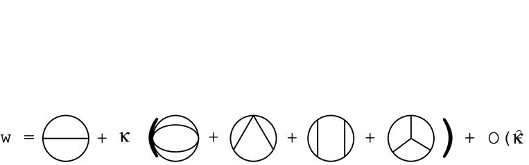
Figure 1: Feynman diagrams contributing to the double scaled partition function $\lim_{V\rightarrow\infty}(\ln Z)/(V\Lambda^{2})$ up to terms of order $\kappa$.

References

- [1] J. Polchinski, String Theory, two volumes, Cambridge University Press 1998.
- [2] É. Brézin, C. Itzykson, G. Parisi and J.-B. Zuber, Comm. Math. Phys. 59 (1978) 35.
-
[3]
É. Brézin and V.A. Kazakov, Phys. Lett. B 236 (1990) 144,
M.R. Douglas and S. Shenker, Nucl. Phys. B 355 (1990) 635,
D.J. Gross and A.A. Migdal, Phys. Rev. Lett. 64 (1990) 127. -
[4]
F. David, Nucl. Phys. B 257 (1985) 45,
V.A. Kazakov, Phys. Lett. B 150 (1985) 282,
J. Ambjörn, B. Durhuus and J. Fröhlich, Nucl. Phys. B 257 (1985) 433. - [5] G. ’t Hooft, Nucl. Phys. B 72 (1974) 461.
- [6] P. Di Francesco, P. Ginsparg and J. Zinn-Justin, Phys. Rep. 254 (1995) 1.
- [7] I.R. Klebanov, String theory in two dimensions, Trieste spring school in String Theory and Quantum Gravity 1991, hep-th/9108019.
- [8] É. Brézin and S.R. Wadia editors, The large expansion in quantum field theory and statistical physics, World Scientific 1993.
- [9] F. Ferrari, Nucl. Phys. B 617 (2001) 348.
- [10] F. Ferrari, Large and double scaling limits in two dimensions, NEIP-01-008, PUPT-1997, LPTENS-01/11, hep-th/0202002.
-
[11]
J. Ambjørn, B. Durhuus, and T. Jónsson,
Phys. Lett. B 244 (1990) 403,
S. Nishigaki and T. Yoneya, Nucl. Phys. B 348 (1991) 787,
P. Di Vecchia, M. Kato, and N. Ohta, Nucl. Phys. B 357 (1991) 495,
G.W. Semenoff and R.J. Szabo, Mod. Phys. Lett. A 11 (1996) 1185. -
[12]
J. Zinn-Justin, Phys. Lett. B 257 (1991) 335,
P. Di Vecchia, M. Kato, and N. Ohta, Int. J. Mod. Phys. A 7 (1992) 1391,
G. Eyal, M. Moshe, S. Nishigaki and J. Zinn-Justin, Nucl. Phys. B 470 (1996) 369. -
[13]
M. Moshe, Quantum field theory in singular limits,
Les Houches lecture 1997, hep-th/9812029,
J. Zinn-Justin, Vector models in the large limit: a few applications, lectures at the 11th Taiwan Spring School on Particles and Fields 1997, hep-th/9810198. - [14] G.W. Semenoff and R.J. Szabo, Int. J. Mod. Phys. A 12 (1997) 2135.
-
[15]
F. Ferrari, Phys. Lett. B 496 (2000) 212,
F. Ferrari, J. High Energy Phys. 6 (2001) 57. - [16] F. Ferrari, Nucl. Phys. B 612 (2001) 151.
- [17] P.C. Argyres and M.R. Douglas, Nucl. Phys. B 448 (1995) 93.
- [18] C. Neumann, Journal für die Reine und Angewandte Mathematik 56 (1859) 46.
-
[19]
R. Seznec and J. Zinn-Justin, J. Math. Phys. 20 (1979) 1398,
J. Zinn-Justin, J. Math. Phys. 22 (1981) 511,
R. Damburg, R. Propin and V. Martyshchenko, J. Phys. A 17 (1984) 3493. -
[20]
É. Brézin, C. Itzykson, G. Parisi, J.-B. Zuber,
Comm. Math. Phys. 59 (1978) 35,
É. Brézin, V.A. Kazakov and Al.B. Zamolodchikov, Nucl. Phys. B 338 (1990) 673,
D. Gross and M. Milkovic, Phys. Lett. B 238 (1990) 217,
G. Parisi, Phys. Lett. B 238 (1990) 209,
P. Ginsparg and J. Zinn-Justin, Phys. Lett. B 240 (1990) 333.