Hard Thermal Effects in Noncommutative ${\rm U}(N)\;$Yang-Mills Theory

F. T. Brandta, J. Frenkela and D. G. C. McKeona,b a Instituto de FΓ­sica, Universidade de SΓ£o Paulo, SΓ£o Paulo, SP 05315-970, BRAZIL b Department of Applied Mathematics, The University of Western Ontario, London, ON N6A5B7, CANADA
Abstract

We study the behaviour of the two- and three-point thermal Green functions, to one loop order in noncommutative ${\rm U}(N)\;$Yang-Mills theory, at temperatures $T$ much higher than the external momenta $p$. We evaluate the amplitudes for small and large values of the variable $\theta\,p\,T$ ($\theta$ is the noncommutative parameter) and exactly compute the static gluon self-energy for all values of $\theta\,p\,T$. We show that these gluon functions, which have a leading $T^{2}$ behaviour, are gauge independent and obey simple Ward identities. We argue that these properties, together with the results for the lowest order amplitudes, may be sufficient to fix uniquely the hard thermal loop effective action of the noncommutative theory.

pacs:
11.15.-q

I Introduction

Noncommutative manifolds have been used in physics for quite some time Groenewold:1946 and were more recently applied in the context of string theories Connes:1998crSeiberg:1999vs . In certain circumstances, the low-energy behaviour of these theories may be described in terms of gauge fields defined on a space-time where the coordinates do not commute, so that

$$\left[x_{\mu},x_{\nu}\right]=i\,\theta_{\mu\nu}.$$ (1)

The antisymmetric tensor $\theta_{\mu\nu}$, which has the canonical dimension of inverse mass squared, is assumed to be independent of the space-time coordinates. Such gauge field theories are non-local and exhibit many intriguing properties, which have been much studied in recent years (for reviews and a complete list of references see, for example, Douglas:2001ba ; Szabo:2001kg . In particular, several thermal effects in noncommutative theories have been already examined in a series of interesting papers Arcioni:1999hw ; Fischler:2000fv ; Fischler:2000bp ; Landsteiner:2000bwlandsteiner:2001ky .

In gauge theories at finite temperature, a consistent perturbative expansion requires the resummation of a set of diagrams called hard thermal loops braaten:1990azBraaten:1990kk . These arise from one-loop diagrams in the region where the internal momenta are of order of the temperature $T$, which is large compared with all the external momenta. The purpose of this work is to study in the non-commutative ${\rm U}(N)\;$Yang-Mills theory, the high temperature behaviour of the two- and three-point gluon functions. Our method of calculation employs an analytic continuation of the imaginary-time formalism kapusta:book89lebellac:book96das:book97 . Using this approach, we relate the Green functions to forward scattering amplitudes of on-shell thermal particles, a technique that has been previously applied in the ${\rm SU}(N)\;$gauge theory as well as in gravity frenkel:1991ts ; brandt:1993dk ; brandt:1997se . In contrast to the situation in the commutative theory, where the hard thermal loop contributions are completely determined in the region where $T\gg p$, one has to consider in the noncommutative case also the value of the independent parameter $\theta\,p\,T$. For arbitrary values of this parameter, the explicit calculation of these non-local amplitudes is, in general, very difficult. Only in certain limiting cases, such as $\theta\,p\,T\ll 1$ or $\theta\,p\,T\gg 1$, is that their evaluation becomes more transparent. An exception occurs in the static case, where one can evaluate, as shown in section II, the gluon self-energy Πμ​νA​BsuperscriptsubscriptΞ πœ‡πœˆπ΄π΅\Pi_{\mu\nu}^{AB} in a closed form for all values of $\theta\,p\,T$. The corresponding result shows a significant difference from the behaviour in the commutative case, where only the Ξ 00A​BsuperscriptsubscriptΞ 00𝐴𝐡\Pi_{00}^{AB} component survives in the static limit. On the other hand, in the noncommutative theory, we find that also the Ξ i​jA​BsuperscriptsubscriptΠ𝑖𝑗𝐴𝐡\Pi_{ij}^{AB} components receives leading $T^{2}$ contributions in the static case. This behaviour reflects the effect of extra magnetic fields which are induced by the noncommutative character of the theory. Furthermore, we show in the section II that the gluon self-energy is generally transverse with respect to the external momenta, and that all the $\theta$-dependence resides in the ${\rm U}(1)$ subgroup of ${\rm U}(N)\;$.

The three-point gluon function is discussed in section III, where we also provide its full $\theta$-dependence which arises in both the ${\rm U}(1)$ and ${\rm SU}(N)\;$sectors. Although the inherent angular integrations are extremely involved and cannot be performed in closed form, we demonstrate that, in general, the leading $T^{2}$ contributions to the three-point amplitude are related to those of the two-point function in a manner dictated by the Ward identity.

Our main motivation for this investigation is that, under certain conditions, these gauge invariant amplitudes, together with the Ward identity, may be sufficient to determine the effective action which sums up the effects of all hard thermal loops. We discuss this issue in section IV and present more details on our calculations in the appendices.

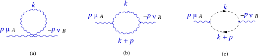
II The two-point function

In accordance with the approach initiated in barton:1990fk and extended to the Yang-Mills theory in frenkel:1991ts we can compute the Feynman graphs of Fig. (1) by considering the on-shell forward scattering amplitudes ${\cal A}_{\mu\nu}^{AB}$ of Fig. (2).

Refer to caption
Figure 1: One-loop diagrams which contribute to the self-energy in the noncommutative ${\rm U}(N)\;$theory. Wavy and dashed lines denote respectively gauge particles and ghosts. The external momenta are inward.

These amplitudes are related to the corresponding two-point function by the equation

Πμ​νA​B=βˆ’1(2​π)3β€‹βˆ«d3​kβ†’2​|kβ†’|​N​(|kβ†’|)β€‹π’œΞΌβ€‹Ξ½A​B|k0=|kβ†’|;A,B=0,1,2,β‹―,N2βˆ’1,formulae-sequencesuperscriptsubscriptΞ πœ‡πœˆπ΄π΅evaluated-at1superscript2πœ‹3superscript𝑑3β†’π‘˜2β†’π‘˜π‘β†’π‘˜superscriptsubscriptπ’œπœ‡πœˆπ΄π΅subscriptπ‘˜0β†’π‘˜π΄π΅012β‹―superscript𝑁21\Pi_{\mu\nu}^{AB}=-{1\over(2\pi)^{3}}\int{d^{3}\vec{k}\over 2\,|\vec{k}|}N(|\vec{k}|)\left.{\cal A}_{\mu\nu}^{AB}\right|_{k_{0}=|\vec{k}|};\;\;\;\;A,B=0,1,2,\cdots,N^{2}-1, (2)

where

$$N(|\vec{k}|)={1\over{\rm e}^{|\vec{k}|/T}-1}$$ (3)

is the Bose-Einstein distribution function.

Refer to caption
Figure 2: Forward scattering amplitudes corresponding to the diagrams in Figure 1. The direction of the ghost momentum is to the left (the same as the corresponding internal gluon line). Contributions with $k\rightarrow-k$ are to be understood.

Using the Feynman rules shown in the appendix A, the contribution of the graph of Fig. (2 a) to the forward scattering amplitude is given by

$${B_{AB}^{\mu\nu}}_{(a)}=-3\,g^{2}\eta^{\mu\nu}\left[{\rm Tr\,}D_{A}\,D_{B}\left(1-c_{p}\right)-{\rm Tr\,}F_{A}\,F_{B}\left(1+c_{p}\right)\right].$$ (4)

We are employing the definitions

$${(F_{A})}_{BC}\equiv f_{BAC},\;\;\;{(D_{A})}_{BC}\equiv d_{BAC},$$ (5)

as well as the abbreviations

$$c_{p}\equiv\cos(p\times k),\;\;c_{pq}\equiv\cos(p\times q),\;\;c_{{1\over 2}p}\equiv\cos({1\over 2}p\times k),\;\;s_{{1\over 2}p}\equiv\sin({1\over 2}p\times k),\;\;c_{{1\over 2}p\times q}\equiv\cos({1\over 2}p\times q);\;\;\;p\times q\equiv p_{\mu}\theta^{\mu\nu}q_{\nu}$$ (6)

Using the results (see Armoni:2000xrBonora:2000ga for similar formulas in the context of one-loop renormalization of noncommutative theories)

$\displaystyle{\rm Tr\,}F_{A}\,F_{B}$ $\displaystyle=$ $\displaystyle-N(1-\delta_{A,0})\,\delta_{AB}$
$\displaystyle{\rm Tr\,}D_{A}\,D_{B}$ $\displaystyle=$ $\displaystyle\;\;N(1+\delta_{A,0})\,\delta_{AB}$
$\displaystyle{\rm Tr\,}D_{A}\,F_{B}$ $\displaystyle=$ $\displaystyle 0,$ (7)

Eq. (4) reduces to

$${B_{AB}^{\mu\nu}}_{(a)}=-6\,g^{2}\,N\,\delta_{AB}\eta^{\mu\nu}\left(1-\delta_{A,0}\,c_{p}\right).$$ (8)

From the graph of Fig. (2 bi) we receive a total contribution

$\displaystyle{B_{AB}^{\mu\nu}}_{(bi)}$ $\displaystyle=$ $\displaystyle{g^{2}\over 4}\,N\,\delta_{AB}\left[5p^{2}\eta^{\mu\nu}-2p^{\mu}p^{\nu}+5\left(k^{\mu}p^{\nu}+k^{\nu}p^{\mu}\right)+10k^{\mu}k^{\nu}+2k\cdot p\eta^{\mu\nu}\right]{1\over p^{2}+2\,k\cdot p}$ (9)
$\displaystyle\times$ $\displaystyle\left[D_{A}\,D_{B}(1-c_{p})-F_{A}\,F_{B}(1+c_{p})\right]+(k\rightarrow-k).$

The contribution of Fig. (2 bii) is identical to that of Fig. (2 bi) with the momentum reversed. Consequently, totalling Figs. (2 bi) and (2 bii) results in

$${B_{AB}^{\mu\nu}}_{(b)}={g^{2}}\,N\,\delta_{AB}\left(1-\delta_{A,0}\,c_{p}\right){5p^{2}\eta^{\mu\nu}-2p^{\mu}p^{\nu}+5\left(k^{\mu}p^{\nu}+k^{\nu}p^{\mu}\right)+10k^{\mu}k^{\nu}+2k\cdot p\eta^{\mu\nu}\over p^{2}+2\,k\cdot p}+(k\rightarrow-k).$$ (10)

In a completely analogous fashion, we find that the amplitude receives the following contributions from Figs. (2 ci) and (2 cii),

$${B_{AB}^{\mu\nu}}_{(ci)}=-{g^{2}}\,N\,\delta_{AB}\left(1-\delta_{A,0}\,c_{p}\right){k^{\mu}\left(k+p\right)^{\nu}\over p^{2}+2\,k\cdot p}+(k\rightarrow-k).$$ (11)

and

$${B_{AB}^{\mu\nu}}_{(cii)}=-{g^{2}}\,N\,\delta_{AB}\left(1-\delta_{A,0}\,c_{p}\right){k^{\mu}\left(k-p\right)^{\nu}\over p^{2}-2\,k\cdot p}+(k\rightarrow-k).$$ (12)

In computing (8), (10), (11) and (12) the gauge parameter $\xi$ in Eq. (71) has been taken to be arbitrary, but it cancels completely in the final result for the $T^{2}$ terms. In the regime in which $p\ll k\sim T$, we make the expansion

$${1\over p^{2}+2\,k\cdot p}={1\over 2\,k\cdot p}-{p^{2}\over(2\,k\cdot p)^{2}}+\cdots,$$ (13)

so that at the leading order in $(2\,k\cdot p)^{-1}$, the total contribution to ${\cal A}^{AB}_{\mu\nu}$ coming from (8), (10), (11) and (12) is

$${\cal A}_{\mu\nu}^{AB}=-4g^{2}N\,\delta^{A,B}\,\left[1-\delta^{A,0}\cos(\tilde{p}\cdot k)\right]G_{\mu\nu};\;\;\;\tilde{p}_{\mu}\equiv p^{\nu}\theta_{\nu\mu}$$ (14)

where

$$G_{\mu\nu}={p^{2}k_{\mu}k_{\nu}\over(k\cdot p)^{2}}-{p_{\mu}k_{\nu}+p_{\nu}k_{\mu}\over k\cdot p}+\eta_{\mu\nu}.$$ (15)

One can easily verify that the transversality property

pμ​Πμ​νA​B=0superscriptπ‘πœ‡superscriptsubscriptΞ πœ‡πœˆπ΄π΅0p^{\mu}\Pi_{\mu\nu}^{AB}=0 (16)

is satisfied. Indeed, this is a direct consequence of $p^{\mu}G_{\mu\nu}=0$. Therefore, we can express the self-energy in terms of the following decomposition

Πμ​νA​BsuperscriptsubscriptΞ πœ‡πœˆπ΄π΅\displaystyle\Pi_{\mu\nu}^{AB} $\displaystyle=$ Ξ 1A​B​(Ξ·ΞΌβ€‹Ξ½βˆ’pμ​pΞ½p2)+Ξ 2A​B​(pΞΌβˆ’p2pβ‹…u​uΞΌ)​(pΞ½βˆ’p2pβ‹…u​uΞ½)​1p2superscriptsubscriptΞ 1𝐴𝐡subscriptπœ‚πœ‡πœˆsubscriptπ‘πœ‡subscriptπ‘πœˆsuperscript𝑝2superscriptsubscriptΞ 2𝐴𝐡subscriptπ‘πœ‡superscript𝑝2⋅𝑝𝑒subscriptπ‘’πœ‡subscriptπ‘πœˆsuperscript𝑝2⋅𝑝𝑒subscriptπ‘’πœˆ1superscript𝑝2\displaystyle\Pi_{1}^{AB}\left(\eta_{\mu\nu}-{p_{\mu}p_{\nu}\over p^{2}}\right)+\Pi_{2}^{AB}\left(p_{\mu}-{p^{2}\over p\cdot u}u_{\mu}\right)\left(p_{\nu}-{p^{2}\over p\cdot u}u_{\nu}\right){1\over p^{2}} (17)
$\displaystyle+$ Ξ 3A​B​p2​p~μ​p~Ξ½+Ξ 4A​B​[(pΞΌβˆ’p2pβ‹…u​uΞΌ)​p~Ξ½+(pΞ½βˆ’p2pβ‹…u​uΞ½)​p~ΞΌ],superscriptsubscriptΞ 3𝐴𝐡superscript𝑝2subscript~π‘πœ‡subscript~π‘πœˆsuperscriptsubscriptΞ 4𝐴𝐡delimited-[]subscriptπ‘πœ‡superscript𝑝2⋅𝑝𝑒subscriptπ‘’πœ‡subscript~π‘πœˆsubscriptπ‘πœˆsuperscript𝑝2⋅𝑝𝑒subscriptπ‘’πœˆsubscript~π‘πœ‡\displaystyle\Pi_{3}^{AB}\,p^{2}\tilde{p}_{\mu}\tilde{p}_{\nu}+\Pi_{4}^{AB}\left[\left(p_{\mu}-{p^{2}\over p\cdot u}u_{\mu}\right)\tilde{p}_{\nu}+\left(p_{\nu}-{p^{2}\over p\cdot u}u_{\nu}\right)\tilde{p}_{\mu}\right],

where $u_{\mu}$ represents the heat bath four velocity [$u=(1,0,0,0)$]. A straightforward calculation gives

Ξ 1A​B=Πμμ​A​B+(Οƒ2βˆ’1)​Π00A​Bβˆ’p~μ​p~Ξ½p~2​Πμ​νA​B;Οƒ2≑p02pβ†’2formulae-sequencesuperscriptsubscriptΞ 1𝐴𝐡subscriptsuperscriptΞ πœ‡π΄π΅πœ‡superscript𝜎21superscriptsubscriptΞ 00𝐴𝐡superscript~π‘πœ‡superscript~π‘πœˆsuperscript~𝑝2superscriptsubscriptΞ πœ‡πœˆπ΄π΅superscript𝜎2superscriptsubscript𝑝02superscript→𝑝2\Pi_{1}^{AB}=\Pi^{\mu\;AB}_{\;\;\mu}+({\sigma}^{2}-1)\Pi_{00}^{AB}-{\tilde{p}^{\mu}\tilde{p}^{\nu}\over\tilde{p}^{2}}\Pi_{\mu\nu}^{AB};\;\;\;{\sigma}^{2}\equiv{p_{0}^{2}\over\vec{p}^{2}} (18)
Ξ 2A​B=Οƒ2​Πμμ​A​B+2​σ2​(Οƒ2βˆ’1)​Π00A​Bβˆ’Οƒ2​p~μ​p~Ξ½p~2​Πμ​νA​BsuperscriptsubscriptΞ 2𝐴𝐡superscript𝜎2subscriptsuperscriptΞ πœ‡π΄π΅πœ‡2superscript𝜎2superscript𝜎21superscriptsubscriptΞ 00𝐴𝐡superscript𝜎2superscript~π‘πœ‡superscript~π‘πœˆsuperscript~𝑝2superscriptsubscriptΞ πœ‡πœˆπ΄π΅\Pi_{2}^{AB}={\sigma}^{2}\,\Pi^{\mu\;AB}_{\;\;\mu}+2{\sigma}^{2}({\sigma}^{2}-1)\Pi_{00}^{AB}-{\sigma}^{2}{\tilde{p}^{\mu}\tilde{p}^{\nu}\over\tilde{p}^{2}}\Pi_{\mu\nu}^{AB} (19)
Ξ 3A​B=βˆ’1p~2​p2​Πμμ​A​Bβˆ’Οƒ2βˆ’1p~2​p2​Π00A​B+2​p~μ​p~Ξ½p~4​p2​Πμ​νA​BsuperscriptsubscriptΞ 3𝐴𝐡1superscript~𝑝2superscript𝑝2subscriptsuperscriptΞ πœ‡π΄π΅πœ‡superscript𝜎21superscript~𝑝2superscript𝑝2superscriptsubscriptΞ 00𝐴𝐡2superscript~π‘πœ‡superscript~π‘πœˆsuperscript~𝑝4superscript𝑝2superscriptsubscriptΞ πœ‡πœˆπ΄π΅\Pi_{3}^{AB}=-{1\over\tilde{p}^{2}p^{2}}\Pi^{\mu\;AB}_{\;\;\mu}-{{\sigma}^{2}-1\over\tilde{p}^{2}p^{2}}\Pi_{00}^{AB}+2{\tilde{p}^{\mu}\tilde{p}^{\nu}\over\tilde{p}^{4}p^{2}}\Pi_{\mu\nu}^{AB} (20)
Ξ 4A​B=(Οƒ2βˆ’1)​p0​p~ΞΌp~2​p2​Πμ​0A​B.superscriptsubscriptΞ 4𝐴𝐡superscript𝜎21subscript𝑝0superscript~π‘πœ‡superscript~𝑝2superscript𝑝2superscriptsubscriptΞ πœ‡0𝐴𝐡\Pi_{4}^{AB}=({\sigma}^{2}-1){p_{0}\tilde{p}^{\mu}\over\tilde{p}^{2}p^{2}}\Pi_{\mu 0}^{AB}. (21)

In order to ensure unitarity Douglas:2001ba ; Szabo:2001kg , we have taken

$$\theta_{0\mu}=0.$$ (22)

The computation of the integrals appearing in Eqs. (18) to (21) is carried out in the appendix B. We find

p~μ​Πμ​0A​B=0,superscript~π‘πœ‡superscriptsubscriptΞ πœ‡0𝐴𝐡0\tilde{p}^{\mu}\Pi_{\mu 0}^{AB}=0, (23)
Πμμ​A​B=N​δA,B​g2​T23​[1βˆ’6Ο€2​δA,0β€‹βˆ‘n=1∞1n2+Ο„2],subscriptsuperscriptΞ πœ‡π΄π΅πœ‡π‘superscript𝛿𝐴𝐡superscript𝑔2superscript𝑇23delimited-[]16superscriptπœ‹2superscript𝛿𝐴0superscriptsubscript𝑛11superscript𝑛2superscript𝜏2\Pi^{\mu\;AB}_{\;\;\mu}=N\,\delta^{A,B}\,{g^{2}\,T^{2}\over 3}\left[1-{6\over\pi^{2}}\delta^{A,0}\sum_{n=1}^{\infty}{1\over n^{2}+{\tau}^{2}}\right], (24)
Ξ 00A​BsubscriptsuperscriptΠ𝐴𝐡00\displaystyle\Pi^{AB}_{00} $\displaystyle=$ $\displaystyle{2\,g^{2}N\,\delta^{A,B}\,\,T^{2}\over(2\pi)^{2}}\int_{-1}^{1}d\zeta\left[1-{2{\sigma}\over{\sigma}-\zeta}+{{\sigma}^{2}-1\over({\sigma}-\zeta)^{2}}\right]$ (25)
$\displaystyle\times$ $\displaystyle\left[{\pi^{2}\over 6}-\delta^{A,0}\,\sum_{n=1}^{\infty}{n\over[n^{2}+{\tau}^{2}(1-\zeta^{2})]^{3/2}}\right].$

and

p~μ​p~Ξ½p~2​Πμ​νA​Bsuperscript~π‘πœ‡superscript~π‘πœˆsuperscript~𝑝2superscriptsubscriptΞ πœ‡πœˆπ΄π΅\displaystyle{\tilde{p}^{\mu}\tilde{p}^{\nu}\over\tilde{p}^{2}}\Pi_{\mu\nu}^{AB} $\displaystyle=$ $\displaystyle-{2\,g^{2}N\,\delta^{A,B}\,\,T^{2}\over(2\pi)^{2}}\int_{-1}^{1}d\zeta\,\left\{\left[{{\sigma}^{2}-1\over({\sigma}-\zeta)^{2}}{1-\zeta^{2}\over 2}-1\right]\right.$ (26)
$\displaystyle\times$ $\displaystyle\left[{\pi^{2}\over 6}-\delta^{A,0}\,\sum_{n=1}^{\infty}{n\over[n^{2}+{\tau}^{2}(1-\zeta^{2})]^{3/2}}\right]$
$\displaystyle+$ $\displaystyle\left.\delta^{A,0}{{\sigma}^{2}-1\over({\sigma}-\zeta)^{2}}{1\over 2{\tau}^{2}}\sum_{n=1}^{\infty}{\left(n-\sqrt{n^{2}+{\tau}^{2}(1-\zeta^{2})}\right)^{2}\left(n+2\sqrt{n^{2}+{\tau}^{2}(1-\zeta^{2})}\right)\over\left(n^{2}+{\tau}^{2}(1-\zeta^{2})\right)^{3/2}}\right\},$

We have defined $\tau^{2}\equiv{\tilde{p}}^{2}\,T^{2}=(\theta_{\mu\nu}p^{\nu})^{2}\,T^{2}$. However, in view of condition (22), this parameter is actually independent of the energy $p_{0}$.

As $G_{\mu\nu}$ in Eq. (15) is homogeneous of degree zero in $k$, Πμ​νA​BsuperscriptsubscriptΞ πœ‡πœˆπ΄π΅\Pi_{\mu\nu}^{AB} acquires to leading order an overall factor of $T^{2}$.

We now consider the various limits referred to in the introduction. With the limit $\theta\,p\,T\gg 1$, we see that all terms proportional to $\delta_{A,0}$ vanish, so that non-planar graphs no longer contribute. This leaves us with some straightforward integration that leads to

Πμμ​A​B=N​δA,B​g2​T23,subscriptsuperscriptΞ πœ‡π΄π΅πœ‡π‘superscript𝛿𝐴𝐡superscript𝑔2superscript𝑇23\Pi^{\mu\;AB}_{\;\;\mu}=N\,\delta^{A,B}\,{g^{2}\,T^{2}\over 3}, (27)
Ξ 00A​B=N​δA,B​g2​T23​(1βˆ’Οƒ2​log⁑σ+1Οƒβˆ’1)superscriptsubscriptΞ 00𝐴𝐡𝑁superscript𝛿𝐴𝐡superscript𝑔2superscript𝑇231𝜎2𝜎1𝜎1\Pi_{00}^{AB}=N\,\,\delta^{A,B}\,{g^{2}\,T^{2}\over 3}\left(1-{{\sigma}\over 2}\log{{{\sigma}+1\over{\sigma}-1}}\right) (28)

and

p~μ​p~Ξ½p~2​Πμ​νA​B=βˆ’N​δA,B​g2​T23​σ2​[12​(Οƒ2βˆ’1)​log⁑σ+1Οƒβˆ’1βˆ’Οƒ]superscript~π‘πœ‡superscript~π‘πœˆsuperscript~𝑝2superscriptsubscriptΞ πœ‡πœˆπ΄π΅π‘superscript𝛿𝐴𝐡superscript𝑔2superscript𝑇23𝜎2delimited-[]12superscript𝜎21𝜎1𝜎1𝜎{\tilde{p}^{\mu}\tilde{p}^{\nu}\over\tilde{p}^{2}}\Pi_{\mu\nu}^{AB}=-N\delta^{A,B}\,{g^{2}\,T^{2}\over 3}{{\sigma}\over 2}\left[{1\over 2}({\sigma}^{2}-1)\log{{{\sigma}+1\over{\sigma}-1}}-{\sigma}\right] (29)

Furthermore, in the limit $\theta\,p\,T\ll 1$, it is possible to extract the contribution to the sums in Eqs. (24) to (26) that are of leading order in ${\tau}^{2}$. Using the standard results for the Riemann zeta function, $\zeta(2)=\pi^{2}/6$ and $\zeta(4)=\pi^{4}/90$, we find that

Πμμ​A​Bβ‰ˆN​δA,B​g2​T23​[1βˆ’Ξ΄A,0+(π​τ)215​δA,0],subscriptsuperscriptΞ πœ‡π΄π΅πœ‡π‘superscript𝛿𝐴𝐡superscript𝑔2superscript𝑇23delimited-[]1superscript𝛿𝐴0superscriptπœ‹πœ215superscript𝛿𝐴0\Pi^{\mu\;AB}_{\;\;\mu}\approx N\,\delta^{A,B}\,{g^{2}\,T^{2}\over 3}\left[1-\delta^{A,0}+{(\pi\,{\tau})^{2}\over 15}\delta^{A,0}\right], (30)
Ξ 00A​BsubscriptsuperscriptΠ𝐴𝐡00\displaystyle\Pi^{AB}_{00} $\displaystyle\approx$ $\displaystyle N\,\delta^{A,B}\,{g^{2}\,T^{2}\over 3}\left[\left(1-{{\sigma}\over 2}\log{{{\sigma}+1\over{\sigma}-1}}\right)(1-\delta^{A,0})\right.$ (31)
$\displaystyle+$ $\displaystyle\left.{(\pi{\tau})^{2}\over 15}\left(2-3{\sigma}^{2}+{3\over 2}{\sigma}({\sigma}^{2}-1)\log{{{\sigma}+1\over{\sigma}-1}}\right)\delta^{A,0}\right]$

and

p~μ​p~Ξ½p~2​Πμ​νA​Bsuperscript~π‘πœ‡superscript~π‘πœˆsuperscript~𝑝2superscriptsubscriptΞ πœ‡πœˆπ΄π΅\displaystyle{\tilde{p}^{\mu}\tilde{p}^{\nu}\over\tilde{p}^{2}}\Pi_{\mu\nu}^{AB} $\displaystyle=$ $\displaystyle-N\,\delta^{A,B}\,\,{g^{2}\,T^{2}\over 3}\left\{{{\sigma}\over 2}\left[{1\over 2}({\sigma}^{2}-1)\log{{{\sigma}+1\over{\sigma}-1}}-{\sigma}\right]\left(1-\delta^{A,0}\right)\right.$
$\displaystyle+$ $\displaystyle\left.{(\pi\,{\tau})^{2}\over 15}\left[1-{15\over 4}{\sigma}^{2}+{9\over 4}{\sigma}^{4}-{9\over 8}{\sigma}\left({\sigma}^{2}-1\right)^{2}\log{{{\sigma}+1\over{\sigma}-1}}\right]\delta^{A,0}\right\}.$

Terms of order ${\tau}^{4}$ and beyond can be similarly computed. We note that all terms involving $\theta$ in Eqs. (30) to (LABEL:34) are proportional to $\delta^{A,0}$.

The integration over $\zeta$ in Eqs. (25) and (26) can be performed and in the static limit when ${\sigma},\,p_{0}\rightarrow 0$. We find in this case that

limΟƒβ†’0Ξ 00A​B=N​δA,B​g2​T23​[1βˆ’6Ο€2β€‹βˆ‘n=1∞n2(n2+Ο„2)2​δA,0],subscriptβ†’πœŽ0superscriptsubscriptΞ 00𝐴𝐡𝑁superscript𝛿𝐴𝐡superscript𝑔2superscript𝑇23delimited-[]16superscriptπœ‹2superscriptsubscript𝑛1superscript𝑛2superscriptsuperscript𝑛2superscript𝜏22superscript𝛿𝐴0\lim_{{\sigma}\rightarrow 0}\Pi_{00}^{AB}=N\,\delta^{A,B}\,{g^{2}\,T^{2}\over 3}\left[1-{6\over\pi^{2}}\sum_{n=1}^{\infty}{n^{2}\over(n^{2}+{\tau}^{2})^{2}}\,\delta^{A,0}\right], (33)
limΟƒβ†’0p~μ​p~Ξ½p~2​Πμ​νA​B=βˆ’2​N​δA,B​g2​T2Ο€2​δA,0β€‹βˆ‘n=1βˆžΟ„2(n2+Ο„2)2.subscriptβ†’πœŽ0superscript~π‘πœ‡superscript~π‘πœˆsuperscript~𝑝2superscriptsubscriptΞ πœ‡πœˆπ΄π΅2𝑁superscript𝛿𝐴𝐡superscript𝑔2superscript𝑇2superscriptπœ‹2superscript𝛿𝐴0superscriptsubscript𝑛1superscript𝜏2superscriptsuperscript𝑛2superscript𝜏22\lim_{{\sigma}\rightarrow 0}{\tilde{p}^{\mu}\tilde{p}^{\nu}\over\tilde{p}^{2}}\Pi_{\mu\nu}^{AB}=-2\,N\,\delta^{A,B}\,{g^{2}\,T^{2}\over\pi^{2}}\,\delta^{A,0}\,\sum_{n=1}^{\infty}{{\tau}^{2}\over(n^{2}+{\tau}^{2})^{2}}. (34)

(Of course, Eq. (24) remains unchanged in the static limit.) The sums appearing in Eqs. (24), (33) and (34) are standard gradshteyn :

$$\sum_{n=1}^{\infty}{1\over n^{2}+a^{2}}={\pi\over 2\,a}{\rm coth}(\pi\,a)-{1\over 2\,a^{2}},$$ (35)
$$\sum_{n=1}^{\infty}{1\over(n^{2}+a^{2})^{2}}={\pi\over 4\,a^{3}}{\rm coth}(\pi\,a)+{\pi^{2}\over 4\,a^{2}}{\rm csch}^{2}(\pi\,a)-{1\over 2\,a^{4}}.$$ (36)

We consequently are led to

Πμμ​A​B=N​δA,B​g2​T23​[1βˆ’3​(1π​τ​coth⁑(π​τ)βˆ’1(π​τ)2)​δA,0],subscriptsuperscriptΞ πœ‡π΄π΅πœ‡π‘superscript𝛿𝐴𝐡superscript𝑔2superscript𝑇23delimited-[]131πœ‹πœhyperbolic-cotangentπœ‹πœ1superscriptπœ‹πœ2superscript𝛿𝐴0\Pi^{\mu\;AB}_{\;\;\mu}=N\,\delta^{A,B}{g^{2}\,T^{2}\over 3}\left[1-3\left({1\over\pi\,{\tau}}\coth(\pi{\tau})-{1\over(\pi\,{\tau})^{2}}\right)\delta^{A,0}\right], (37)
limΟƒβ†’0Ξ 00A​B=N​δA,B​g2​T23​{1βˆ’32​[1π​τ​coth⁑(π​τ)βˆ’csch2​(π​τ)]​δA,0}subscriptβ†’πœŽ0superscriptsubscriptΞ 00𝐴𝐡𝑁superscript𝛿𝐴𝐡superscript𝑔2superscript𝑇23132delimited-[]1πœ‹πœhyperbolic-cotangentπœ‹πœsuperscriptcsch2πœ‹πœsuperscript𝛿𝐴0\lim_{{\sigma}\rightarrow 0}\Pi_{00}^{AB}=N\,\delta^{A,B}\,{g^{2}\,T^{2}\over 3}\left\{1-{3\over 2}\left[{1\over\pi{\tau}}\coth(\pi{\tau})-{\rm csch}^{2}(\pi{\tau})\right]\delta^{A,0}\right\} (38)

and

limΟƒβ†’0p~μ​p~Ξ½p~2​Πμ​νA​Bsubscriptβ†’πœŽ0superscript~π‘πœ‡superscript~π‘πœˆsuperscript~𝑝2superscriptsubscriptΞ πœ‡πœˆπ΄π΅\displaystyle\lim_{{\sigma}\rightarrow 0}{\tilde{p}^{\mu}\tilde{p}^{\nu}\over\tilde{p}^{2}}\Pi_{\mu\nu}^{AB} $\displaystyle=$ $\displaystyle-N\,\delta^{A,B}\,{g^{2}\,T^{2}}{{\rm csch}^{2}(\pi{\tau})\over 2\,(\pi\,{\tau})^{2}}\left[1+(\pi{\tau})^{2}-{\rm cosh}(2\pi{\tau})+{\pi{\tau}\over 2}{\rm sinh}(2\pi{\tau})\right]\,\delta^{A,0}.$ (39)

From the previous results we can now obtain the static limit of Eqs. (18), (19) and (20) (we show in the appendix that Ξ 4A​B=0superscriptsubscriptΞ 4𝐴𝐡0\Pi_{4}^{AB}=0). From Eq. (18), we have

limΟƒβ†’0Ξ 1A​B=limΟƒβ†’0Πμμ​A​Bβˆ’limΟƒβ†’0Ξ 00A​Bβˆ’limΟƒβ†’0p~μ​p~Ξ½p~2​Πμ​νA​B.subscriptβ†’πœŽ0superscriptsubscriptΞ 1𝐴𝐡subscriptβ†’πœŽ0subscriptsuperscriptΞ πœ‡π΄π΅πœ‡subscriptβ†’πœŽ0subscriptsuperscriptΠ𝐴𝐡00subscriptβ†’πœŽ0superscript~π‘πœ‡superscript~π‘πœˆsuperscript~𝑝2superscriptsubscriptΞ πœ‡πœˆπ΄π΅\lim_{{\sigma}\rightarrow 0}\Pi_{1}^{AB}=\lim_{{\sigma}\rightarrow 0}\Pi^{\mu\;\;AB}_{\;\;\mu}-\lim_{{\sigma}\rightarrow 0}\Pi^{AB}_{00}-\lim_{{\sigma}\rightarrow 0}{\tilde{p}^{\mu}\tilde{p}^{\nu}\over\tilde{p}^{2}}\Pi_{\mu\nu}^{AB}. (40)

Using Eqs. (24), (33) and (34), we obtain

limΟƒβ†’0Ξ 1A​B=0.subscriptβ†’πœŽ0superscriptsubscriptΞ 1𝐴𝐡0\lim_{{\sigma}\rightarrow 0}\Pi_{1}^{AB}=0. (41)

The static limit of Ξ 2subscriptΞ 2\Pi_{2} in Eq. (19) behaves as ${\sigma}^{2}$. Therefore, Ξ 2subscriptΞ 2\Pi_{2} will contribute only to Ξ 00A​BsuperscriptsubscriptΞ 00𝐴𝐡\Pi_{00}^{AB} in Eq. (17) but not to either Ξ i​jA​BsuperscriptsubscriptΠ𝑖𝑗𝐴𝐡\Pi_{ij}^{AB} or Ξ 0​iA​BsuperscriptsubscriptΞ 0𝑖𝐴𝐡\Pi_{0i}^{AB} ($i,j=1,2,3$) [of course, we do not need Ξ 2subscriptΞ 2\Pi_{2} in order to obtain Ξ 00A​BsuperscriptsubscriptΞ 00𝐴𝐡\Pi_{00}^{AB} which has already been obtained explicitly in Eq. (38)]. Using Eq. (20), we obtain for the static limit of Ξ 3subscriptΞ 3\Pi_{3}

limΟƒβ†’0Ξ 3A​Bsubscriptβ†’πœŽ0superscriptsubscriptΞ 3𝐴𝐡\displaystyle\lim_{{\sigma}\rightarrow 0}\Pi_{3}^{AB} $\displaystyle=$ βˆ’1|p~β†’|2​|pβ†’|2​limΟƒβ†’0[Πμμ​A​Bβˆ’Ξ 00A​Bβˆ’2​p~μ​p~Ξ½p~2​Πμ​νA​B]1superscriptβ†’~𝑝2superscript→𝑝2subscriptβ†’πœŽ0delimited-[]subscriptsuperscriptΞ πœ‡π΄π΅πœ‡superscriptsubscriptΞ 00𝐴𝐡2superscript~π‘πœ‡superscript~π‘πœˆsuperscript~𝑝2superscriptsubscriptΞ πœ‡πœˆπ΄π΅\displaystyle-{1\over|\vec{\tilde{p}}|^{2}|{\vec{p}}|^{2}}\lim_{{\sigma}\rightarrow 0}\left[\Pi^{\mu\;\;AB}_{\;\;\mu}-\Pi_{00}^{AB}-2{\tilde{p}^{\mu}\tilde{p}^{\nu}\over\tilde{p}^{2}}\Pi_{\mu\nu}^{AB}\right] (42)
$\displaystyle=$ βˆ’3​limΟƒβ†’0p~μ​p~Ξ½p~2​Πμ​νA​B3subscriptβ†’πœŽ0superscript~π‘πœ‡superscript~π‘πœˆsuperscript~𝑝2superscriptsubscriptΞ πœ‡πœˆπ΄π΅\displaystyle-3\lim_{{\sigma}\rightarrow 0}{\tilde{p}^{\mu}\tilde{p}^{\nu}\over\tilde{p}^{2}}\Pi_{\mu\nu}^{AB}

Finally, using Eq. (39) in Eq. (42) as well as simple functional relations involving the hyperbolic functions, we obtain

limΟƒβ†’0Ξ 3A​B=N​δA,B​δA,0​3​g2​T22​[1sinh2​(π​τ)βˆ’2(π​τ)2+cosh​(π​τ)π​τ​sinh​(π​τ)].subscriptβ†’πœŽ0superscriptsubscriptΞ 3𝐴𝐡𝑁superscript𝛿𝐴𝐡superscript𝛿𝐴03superscript𝑔2superscript𝑇22delimited-[]1superscriptsinh2πœ‹πœ2superscriptπœ‹πœ2coshπœ‹πœπœ‹πœsinhπœ‹πœ\lim_{{\sigma}\rightarrow 0}\Pi_{3}^{AB}=N\,\delta^{A,B}\,\delta^{A,0}{3\,g^{2}\,T^{2}\over 2}\left[{1\over{\rm sinh}^{2}(\pi\,{\tau})}-{2\over(\pi\,{\tau})^{2}}+{{\rm cosh}(\pi\,{\tau})\over\pi\,{\tau}{\rm sinh}(\pi\,{\tau})}\right]. (43)

Inserting Eq. (43) into Eq. (17) one can easily obtain Ξ i​jA​BsuperscriptsubscriptΠ𝑖𝑗𝐴𝐡\Pi_{i\,j}^{AB}. It is interesting to note that in commutative Yang-Mills theory Ξ 00A​BsuperscriptsubscriptΞ 00𝐴𝐡\Pi_{00}^{AB} is non-zero but Ξ i​jA​BsuperscriptsubscriptΠ𝑖𝑗𝐴𝐡\Pi_{ij}^{AB} vanishes, while in the noncommutative case, we see from Eq. (43) that Ξ i​jA​Bβ‰ 0superscriptsubscriptΠ𝑖𝑗𝐴𝐡0\Pi_{ij}^{AB}\neq 0 when then colour $A$ is in the ${\rm U}(1)$ sector ($A=0$). This is consistent with the additional magnetic interactions appearing in the initial Lagrangian. However, since Ξ i​iA​B​(p0=0,pβ†’β†’0)=0subscriptsuperscriptΠ𝐴𝐡𝑖𝑖formulae-sequencesubscript𝑝00→→𝑝00\Pi^{AB}_{ii}(p_{0}=0,\vec{p}\rightarrow 0)=0, the magnetic mass vanishes also in the noncommutative theory.

It also proves possible to examine Πμ​νA​BsuperscriptsubscriptΞ πœ‡πœˆπ΄π΅\Pi_{\mu\nu}^{AB} in the long wave length limit $\sigma\rightarrow\infty$ and $\tau\rightarrow 0$. In this case, we see from Eqs. (24), (25) and (26) that

Ξ 00A​BsuperscriptsubscriptΞ 00𝐴𝐡\displaystyle\Pi_{00}^{AB} $\displaystyle\longrightarrow$ $\displaystyle 0,$
Ξ ΞΌA​B​μsuperscriptsubscriptΞ πœ‡π΄π΅πœ‡\displaystyle\Pi_{\mu}^{AB\,\mu} $\displaystyle\longrightarrow$ $\displaystyle N\delta^{A,B}{g^{2}\,T^{2}\over 3}\left(1-\delta^{A,0}\right),$
p~μ​p~Ξ½p~2​Πμ​νA​Bsuperscript~π‘πœ‡superscript~π‘πœˆsuperscript~𝑝2superscriptsubscriptΞ πœ‡πœˆπ΄π΅\displaystyle{\tilde{p}^{\mu}\tilde{p}^{\nu}\over{\tilde{p}}^{2}}\Pi_{\mu\nu}^{AB} $\displaystyle\longrightarrow$ $\displaystyle N\delta^{A,B}{g^{2}\,T^{2}\over 9}\left(1-\delta^{A,0}\right).$ (44)

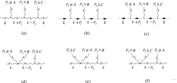
III The three-point function

The Feynman graphs we consider are those of Fig. 3. These are associated with the amplitudes of Fig. 4. The calculation of the diagrams in figure 4 is straightforward but very tedious. After some algebra, the amplitude in figure 4 (a) can be written as (we have employed the Maple version of the symbolic computer package HIP hsieh:1992ti )

$${\cal A}_{\mu\nu\lambda}^{gl\;ABC}=\left[\sin\left({p_{1}\times p_{2}\over 2}\right)C_{\sin}^{gl\;ABC}+\cos\left({p_{1}\times p_{2}\over 2}\right)C_{\cos}^{gl\;ABC}\right]L^{gl}_{\mu\nu\lambda}$$ (45)

Similarly the sum of the diagrams in figures 4 (b) and 4 (c) give

$${\cal A}_{\mu\nu\lambda}^{gh\;ABC}=\left[\sin\left({p_{1}\times p_{2}\over 2}\right)C_{\sin}^{gh\;ABC}+\cos\left({p_{1}\times p_{2}\over 2}\right)C_{\cos}^{gh\;ABC}\right]L^{gh}_{\mu\nu\lambda}$$ (46)
Refer to caption
Figure 3: One-loop diagrams which contribute to the three-point function.

The factors $C_{\sin}^{gl\;ABC}$, $C_{\cos}^{gl\;ABC}$, $C_{\sin}^{gh\;ABC}$ and $C_{\cos}^{gh\;ABC}$ are trigonometric functions of the internal momentum $k$ and involve the colour factors. At any specific order in the hard thermal loop expansion, the Lorentz factors $L^{gl}_{\mu\nu\lambda}$ and $L^{gh}_{\mu\nu\lambda}$ will be odd or even in $k$. Terms which are odd in $k$ will be multiplied by the following antisymmetric factors

$\displaystyle A_{\sin}^{gl\;ABC}={1\over 2}\left(C_{\sin}^{gl\;ABC}(k)-C_{\sin}^{gl\;ABC}(-k)\right)$
$\displaystyle A_{\sin}^{gh\;ABC}={1\over 2}\left(C_{\sin}^{gh\;ABC}(k)-C_{\sin}^{gh\;ABC}(-k)\right)$
$\displaystyle A_{\cos}^{gl\;ABC}={1\over 2}\left(C_{\cos}^{gl\;ABC}(k)-C_{\cos}^{gl\;ABC}(-k)\right)$
$\displaystyle A_{\cos}^{gh\;ABC}={1\over 2}\left(C_{\cos}^{gh\;ABC}(k)-C_{\cos}^{gh\;ABC}(-k)\right)$ (47)

Terms which are even in $k$ will be multiplied by the following symmetric factors

$\displaystyle S_{\sin}^{gl\;ABC}={1\over 2}\left(C_{\sin}^{gl\;ABC}(k)+C_{\sin}^{gl\;ABC}(-k)\right)$
$\displaystyle S_{\sin}^{gh\;ABC}={1\over 2}\left(C_{\sin}^{gh\;ABC}(k)+C_{\sin}^{gh\;ABC}(-k)\right)$
$\displaystyle S_{\cos}^{gl\;ABC}={1\over 2}\left(C_{\cos}^{gl\;ABC}(k)+C_{\cos}^{gl\;ABC}(-k)\right)$
$\displaystyle S_{\cos}^{gh\;ABC}={1\over 2}\left(C_{\cos}^{gh\;ABC}(k)+C_{\cos}^{gh\;ABC}(-k)\right)$ (48)
Refer to caption
Figure 4: Forward scattering amplitudes corresponding to the diagrams in Figure 3. The direction of the ghost momentum is the same as the corresponding internal gluon line. Permutations of the vertices are understood.

A straightforward calculation gives

$\displaystyle A_{\sin}^{gl\;ABC}$ $\displaystyle=$ $\displaystyle-{\rm Tr\,}\left[F^{A}\,D^{B}\,D^{C}\,c_{{1\over 2}p_{1}}\,c_{{1\over 2}p_{2}}\,\,s_{{1\over 2}p_{3}}\,-F^{A}\,F^{B}\,F^{C}\,c_{{1\over 2}p_{1}}\,s_{{1\over 2}p_{2}}\,\,c_{{1\over 2}p_{3}}\,\right.$ (49)
$\displaystyle\;\;\;\;\;\left.+F^{C}\,D^{A}\,D^{B}\,s_{{1\over 2}p_{1}}\,\,c_{{1\over 2}p_{2}}\,\,c_{{1\over 2}p_{3}}\,-F^{B}\,D^{C}\,D^{A}\,s_{{1\over 2}p_{1}}\,\,s_{{1\over 2}p_{2}}\,\,s_{{1\over 2}p_{3}}\,\right],$

where we are using the abbreviations defined in Eqs. (5) and (6). Using the relations Armoni:2000xrBonora:2000ga

$${\rm Tr\,}F^{A}\,F^{B}\,F^{C}=-{N\over 2}f^{ABC}=-{\rm Tr\,}F^{A}\,D^{B}\,D^{C},$$ (50)

as well as the cyclic property of the trace, we can write

$\displaystyle A_{\sin}^{gl\;ABC}$ $\displaystyle=$ $\displaystyle-{N\over 2}f^{ABC}\left[\,c_{{1\over 2}p_{1}}\,c_{{1\over 2}p_{2}}\,\,s_{{1\over 2}p_{3}}\,+\,c_{{1\over 2}p_{1}}\,s_{{1\over 2}p_{2}}\,\,c_{{1\over 2}p_{3}}\,\right.$ (51)
$\displaystyle\;\;\;\;\;\;\;\;\;\;\;\;\;\;\left.+\,s_{{1\over 2}p_{1}}\,\,c_{{1\over 2}p_{2}}\,\,c_{{1\over 2}p_{3}}\,\ -\,s_{{1\over 2}p_{1}}\,\,s_{{1\over 2}p_{2}}\,\,s_{{1\over 2}p_{3}}\,\right]$
$\displaystyle=$ $\displaystyle-{N\over 2}f^{ABC}\sin\left({p_{1}+p_{2}+p_{3}\over 2}\times k\right)=0,$

where we have used the momentum conservation $p_{1}+p_{2}+p_{3}=0$. A similar calculation for the ghost part also gives

$$A_{\sin}^{gh\;ABC}=0.$$ (52)

The Eqs. (51) and (52) imply that there is no contribution which is odd in the temperature $T$ and proportional to $\sin[(p_{1}\times p_{2})/2]$.

Let us now consider the coefficients of $\cos[(p_{1}\times p_{2})/2]$ which are antisymmetric functions of $k$, namely $A_{\cos}^{gl\;ABC}$ and $A_{\cos}^{gh\;ABC}$. The colour traces which are involved now are Armoni:2000xrBonora:2000ga

$\displaystyle{\rm Tr\,}D^{A}D^{B}D^{C}$ $\displaystyle=$ $\displaystyle{N\over 2}\eta_{ABC}\,d^{ABC};\;\;\;\eta_{ABC}\equiv d_{A}d_{B}d_{C}-4\delta_{A+B+C,0}$
$\displaystyle{\rm Tr\,}F^{A}F^{B}D^{C}$ $\displaystyle=$ $\displaystyle-{N\over 2}c_{A}c_{B}d_{C}\,d^{ABC};\;\;c_{A}\equiv 1-\delta_{A,0};\;\;d_{A}\equiv 1+\delta_{A,0}$ (53)

A straightforward calculation gives

$\displaystyle A_{\cos}^{gl\;ABC}$ $\displaystyle=$ $\displaystyle-{\rm Tr\,}\left[F^{A}\,F^{B}\,D^{C}\,c_{{1\over 2}p_{1}}\,c_{{1\over 2}p_{2}}\,\,s_{{1\over 2}p_{3}}\,\right.\left.+D^{A}\,F^{B}\,F^{C}\,s_{{1\over 2}p_{1}}\,\,c_{{1\over 2}p_{2}}\,\,c_{{1\over 2}p_{3}}\,\right.$ (54)
$\displaystyle\;\;\;\;\;\left.+F^{C}\,F^{A}\,D^{B}\,c_{{1\over 2}p_{1}}\,s_{{1\over 2}p_{2}}\,\,c_{{1\over 2}p_{3}}\,+D^{A}\,D^{B}\,D^{C}\,s_{{1\over 2}p_{1}}\,\,s_{{1\over 2}p_{2}}\,\,s_{{1\over 2}p_{3}}\,\right]$

In contrast to the antisymmetric coefficient of $\sin[(p_{1}\times p_{2})/2]$, $A_{\cos}^{gl\;ABC}$ does not vanish by itself. Using trace cyclicity, one can write

$\displaystyle A_{\cos}^{gl\;ABC}$ $\displaystyle=$ $\displaystyle{\rm Tr\,}\left[-F^{A}\,F^{B}\,D^{C}\,c_{{1\over 2}p_{1}}\,c_{{1\over 2}p_{2}}\,\,s_{{1\over 2}p_{3}}\,+{1\over 3}D^{A}\,D^{B}\,D^{C}\,s_{{1\over 2}p_{1}}\,\,s_{{1\over 2}p_{2}}\,\,s_{{1\over 2}p_{3}}\,\right]$ (55)
$\displaystyle+$ $\displaystyle{\rm cyclic\;\;\;permut.}$

Let us consider the specific case of the superleading contribution, which would be proportional to $T^{3}$. The Lorentz factor for this piece is the same for the gluon and for the ghost diagrams, being proportional to [see the diagrams in figure 4 (a), (b) and (c)],

$${k_{\mu}k_{\nu}k_{\lambda}\over k\cdot p_{1}k\cdot p_{3}}$$ (56)

Including the colour and the $\cos\left({p_{1}\times p_{2}\over 2}\right)$ factors, this leads to a contribution

$$\cos\left({p_{1}\times p_{2}\over 2}\right)A_{\cos}^{gl\;ABC}(p_{1},p_{2},p_{3})k_{\mu}k_{\nu}k_{\lambda}\,{1\over k\cdot p_{1}k\cdot p_{3}}$$ (57)

The only part of Eq. (57) which will change when we add together all cyclic permutations is the denominator. Using momentum conservation, we have

$${1\over k\cdot p_{1}\;k\cdot p_{3}}+{1\over k\cdot p_{1}\;k\cdot p_{2}}+{1\over k\cdot p_{2}\;k\cdot p_{3}}=0,$$ (58)

and thus we can easily see that the superleading contribution (viz. those that are proportional to $T^{3}$) will vanish. The same property is also true for the ghost diagram. This cancellation of the superleading contribution is similar to what happens in QCD frenkel:1991ts . However, in the case of noncommutative theories one has to employ the cyclicity property of the colour/trigonometric factor, rather than simply relying in the cancellation which occurs when we add the contributions with $k\rightarrow-k$, as is the case in QCD. (In QCD, there is no $k$-dependent trigonometric factor which is odd in $k$.)

In a similar way, it is straightforward to show that

$\displaystyle S_{\cos}^{gl\;ABC}$ $\displaystyle=$ $\displaystyle{\rm Tr\,}\left[F^{A}\,F^{B}\,F^{C}\,c_{{1\over 2}p_{1}}\,c_{{1\over 2}p_{2}}\,\,c_{{1\over 2}p_{3}}+F^{A}\,D^{B}\,D^{C}\,c_{{1\over 2}p_{1}}\,\,s_{{1\over 2}p_{2}}\,\,s_{{1\over 2}p_{3}}\,\right.$ (59)
$\displaystyle\;\;\;\;\;\left.+F^{B}\,D^{C}\,D^{A}\,s_{{1\over 2}p_{1}}\,c_{{1\over 2}p_{2}}\,\,s_{{1\over 2}p_{3}}+F^{C}\,D^{A}\,D^{B}\,s_{{1\over 2}p_{1}}\,\,s_{{1\over 2}p_{2}}\,\,c_{{1\over 2}p_{3}}\,\right]$
$\displaystyle=$ $\displaystyle-{N\over 2}f^{ABC}\cos\left[{1\over 2}(p_{1}+p_{2}+p_{3})\times k\right]=-{N\over 2}f^{ABC},$
$\displaystyle S_{\cos}^{gh\;ABC}$ $\displaystyle=$ $\displaystyle{\rm Tr\,}\left[F^{A}\,F^{B}\,F^{C}\left(c_{{1\over 2}p_{1}}^{2}\,c_{{1\over 2}p_{3}}^{2}-c_{{1\over 2}p_{1}}\,c_{{1\over 2}p_{3}}s_{{1\over 2}p_{1}}\,s_{{1\over 2}p_{3}}\right)-F^{A}\,D^{B}\,D^{C}\left(c_{{1\over 2}p_{1}}^{2}\,\,s_{{1\over 2}p_{3}}^{2}+c_{{1\over 2}p_{1}}\,c_{{1\over 2}p_{3}}s_{{1\over 2}p_{1}}\,s_{{1\over 2}p_{3}}\right)\right.$ (60)
$\displaystyle\left.-F^{B}\,D^{C}\,D^{A}\left(s_{{1\over 2}p_{1}}^{2}\,s_{{1\over 2}p_{3}}^{2}-c_{{1\over 2}p_{1}}\,c_{{1\over 2}p_{3}}s_{{1\over 2}p_{1}}\,s_{{1\over 2}p_{3}}\right)-F^{C}\,D^{A}\,D^{B}\left(s_{{1\over 2}p_{1}}^{2}\,\,c_{{1\over 2}p_{3}}^{2}+c_{{1\over 2}p_{1}}\,c_{{1\over 2}p_{3}}s_{{1\over 2}p_{1}}\,s_{{1\over 2}p_{3}}\right)\right]$
$\displaystyle=$ $\displaystyle-{N\over 2}f^{ABC},$
$\displaystyle S_{\sin}^{gl\;ABC}$ $\displaystyle=$ $\displaystyle{\rm Tr\,}\left[-F^{A}\,F^{B}\,D^{C}\,c_{{1\over 2}p_{1}}\,s_{{1\over 2}p_{2}}\,\,s_{{1\over 2}p_{3}}-F^{B}\,F^{C}\,D^{A}\,s_{{1\over 2}p_{1}}\,\,s_{{1\over 2}p_{2}}\,\,c_{{1\over 2}p_{3}}\,\right.$ (61)
$\displaystyle\;\;\;\;\;\left.+F^{C}\,F^{A}\,D^{B}\,c_{{1\over 2}p_{1}}\,c_{{1\over 2}p_{2}}\,\,c_{{1\over 2}p_{3}}+D^{A}\,D^{B}\,D^{C}\,s_{{1\over 2}p_{1}}\,\,c_{{1\over 2}p_{2}}\,\,s_{{1\over 2}p_{3}}\,\right]$
$\displaystyle=$ $\displaystyle-{N\over 2}d^{ABC}\left[1+c_{p_{1}}\left(\delta^{A,0}\delta^{B,0}\delta^{C,0}-\delta^{B,0}\delta^{C,0}-\delta^{A,0}\right)\right.$
$\displaystyle\;\;\;\;\;\;\;\;\;\;\;\;\;\;\;\;\;\;\;-\;c_{p_{2}}\left(\delta^{A,0}\delta^{B,0}\delta^{C,0}-\delta^{A,0}\delta^{C,0}-\delta^{B,0}\right)$
$\displaystyle\;\;\;\;\;\;\;\;\;\;\;\;\;\;\;\;\;\;\;\left.-\;c_{p_{3}}\left(\delta^{A,0}\delta^{B,0}\delta^{C,0}-\delta^{A,0}\delta^{B,0}-\delta^{C,0}\right)\right],$

and

$\displaystyle S_{\sin}^{gh\;ABC}$ $\displaystyle=$ $\displaystyle{1\over 4}{\rm Tr\,}\left[F^{A}\,F^{B}\,D^{C}+F^{A}\,D^{B}\,F^{C}+D^{A}\,F^{B}\,F^{C}-D^{A}\,D^{B}\,D^{C}\right.$ (62)
$\displaystyle\;\;\;\;\;+c_{p_{1}}\left(F^{A}\,F^{B}\,D^{C}+F^{A}\,D^{B}\,F^{C}-D^{A}\,F^{B}\,F^{C}+D^{A}\,D^{B}\,D^{C}\right)$
$\displaystyle\;\;\;\;\;+c_{p_{2}}\left(-F^{A}\,F^{B}\,D^{C}+F^{A}\,D^{B}\,F^{C}-D^{A}\,F^{B}\,F^{C}-D^{A}\,D^{B}\,D^{C}\right)$
$\displaystyle\;\;\;\;\;\left.+c_{p_{3}}\left(-F^{A}\,F^{B}\,D^{C}+F^{A}\,D^{B}\,F^{C}+D^{A}\,F^{B}\,F^{C}+D^{A}\,D^{B}\,D^{C}\right)\right]$
$\displaystyle=$ $\displaystyle-{N\over 2}d^{ABC}\left[1+c_{p_{1}}\left(\delta^{A,0}\delta^{B,0}\delta^{C,0}-\delta^{B,0}\delta^{C,0}-\delta^{A,0}\right)\right.$
$\displaystyle\;\;\;\;\;\;\;\;\;\;\;\;\;\;\;\;\;\;\;-\;c_{p_{2}}\left(\delta^{A,0}\delta^{B,0}\delta^{C,0}-\delta^{A,0}\delta^{C,0}-\delta^{B,0}\right)$
$\displaystyle\;\;\;\;\;\;\;\;\;\;\;\;\;\;\;\;\;\;\;\left.+\;c_{p_{3}}\left(\delta^{A,0}\delta^{B,0}\delta^{C,0}-\delta^{A,0}\delta^{B,0}-\delta^{C,0}\right)\right].$

By Eqs. (59) to (62) it is evident that the full amplitude associated with Figs. 4 (a), (b) and (c) is

$\displaystyle\left.{\cal A}_{\mu\nu\lambda}^{ABC}\right|_{(a),(b),(c)}$ $\displaystyle=$ $\displaystyle-{N\over 2}\left[f^{ABC}\cos\left({p_{1}\times p_{2}\over 2}\right)+d^{ABC}\left(1+O^{ABC}\right)\sin\left({p_{1}\times p_{2}\over 2}\right)\right]$ (63)
$\displaystyle\times$ $\displaystyle\left[L^{gl}_{\mu\nu\lambda}+L^{gh}_{\mu\nu\lambda}\right],$

where

$\displaystyle O^{ABC}$ $\displaystyle=$ $\displaystyle\cos(p_{1}\times k)\left(\delta^{A,0}\delta^{B,0}\delta^{C,0}-\delta^{B,0}\delta^{C,0}-\delta^{A,0}\right)$ (64)
$\displaystyle-$ $\displaystyle\cos(p_{2}\times k)\left(\delta^{A,0}\delta^{B,0}\delta^{C,0}-\delta^{A,0}\delta^{C,0}-\delta^{B,0}\right)$
$\displaystyle+$ $\displaystyle\cos(p_{3}\times k)\left(\delta^{A,0}\delta^{B,0}\delta^{C,0}-\delta^{A,0}\delta^{B,0}-\delta^{C,0}\right)$

is an oscillatory part which gives a subleading contribution for $\theta\,p\,T\gg 1$. Furthermore, explicit computation gives

$\displaystyle L^{gl}_{\mu\nu\lambda}+L^{gh}_{\mu\nu\lambda}$ $\displaystyle=$ $\displaystyle{i\over k\cdot p_{3}}\left[{{4\,{{p_{1}}}^{2}k_{{\mu}}k_{{\nu}}k_{{\lambda}}}\over{{{(k\cdot p_{1})}}^{2}}}+{{4\,k_{{\nu}}k_{{\mu}}{p_{3}}_{{\lambda}}}\over{{k\cdot p_{1}}}}+{{4\,{p_{3}}_{{\nu}}k_{{\mu}}k_{{\lambda}}}\over{{k\cdot p_{1}}}}-k_{{\mu}}\eta_{{\lambda,\nu}}-k_{{\nu}}\eta_{{\lambda,\mu}}\right]$ (65)
$\displaystyle-$ $\displaystyle\left([(\mu,p_{1}),(\lambda,p_{3})]\right)\longleftrightarrow\left([(\lambda,p_{3}),(\mu,p_{1})]\right).$

(As in the case of the two-point function, in the leading thermal contributions, all dependence of the three-point function on the gauge parameter $\xi$ cancels completely.) The full contribution to the three-point function is obtained adding to Eq. (63) two cyclic permutations of $(\mu,p_{1}),\;(\nu,p_{2})\;(\lambda,p_{3})$. In the limit $\theta\,p\,T\gg 1$, when $O^{ABC}$ can be neglected, the colour/trigonometric factor in Eq. (63) does not change under cyclic permutations. Therefore, we can write

$\displaystyle\lim_{(\theta\,p\,T)\rightarrow\infty}\left[\left.{\cal A}_{\mu\nu\lambda}^{ABC}\right|_{(a),(b),(c)}+{\rm cyclic\;\;perm.\;\;of\;}(\mu,p_{1}),\;(\nu,p_{2})\;(\lambda,p_{3})\right]$ $\displaystyle=$ $\displaystyle-{N\over 2}C^{ABC}(p_{1},p_{2})\left[L^{gl}_{\mu\nu\lambda}+L^{gh}_{\mu\nu\lambda}\right]$ (66)
$\displaystyle+$ $\displaystyle{\rm cyclic\;\;perm.\;\;of\;}(\mu,p_{1}),\;(\nu,p_{2})\;(\lambda,p_{3}),$

where $C^{ABC}(p_{1},p_{2})$ is given by Eq. (79). Since the factor $C^{ABC}(p_{1},p_{2})$ does not change under cyclic permutations, the Lorentz factor $L^{gl}_{\mu\nu\lambda}+L^{gh}_{\mu\nu\lambda}$, plus its cyclic permutations simplifies to an expression without terms involving the metric tensor $\eta$, so that the full expression from the diagrams in Figs. 4 (a), (b) and (c) can be written as

$\displaystyle\lim_{(\theta\,p\,T)\rightarrow\infty}\left.{\cal A}_{\mu\nu\lambda}^{ABC}\right|_{(a),(b),(c)}$ $\displaystyle=$ $\displaystyle-{i\,N\,C^{ABC}(p_{1},p_{2})\over k\cdot p_{3}}\left[{k_{\mu}\,k_{\nu}\,k_{\lambda}\,p_{3}^{2}\over(k\cdot p_{1})^{2}}+2{k_{\mu}\,k_{\lambda}\,{p_{3}}_{\nu}\over k\cdot p_{1}}+(\mu\leftrightarrow\nu)\right]$ (67)
$\displaystyle+$ $\displaystyle\left[(A,\mu,p_{1}),(C,\lambda,p_{3})\right]\longleftrightarrow\left[(C,\lambda,p_{3}),(A,\mu,p_{1})\right].$

The remaining contribution, associated with the amplitudes in Figs. 4 (d), (e) and (f), is purely oscillatory and hence will not contribute when $\theta\,p\,T\gg 1$. Including the two identical contributions which arise as a result of reversing the momentum flow of $k$ in Fig. 4 (d), (e), and (f) and also by interchanging the two vertices appearing there, we obtain

$\displaystyle\left.{\cal A}_{\mu\nu\lambda}^{ABC}\right|_{(d),(e),(f)}$ $\displaystyle=$ $\displaystyle-{2\,i\,N}\,d^{ABC}\sin\left({p_{1}\times p_{2}\over 2}\right)\cos(p_{1}\times k)\left(\delta^{A,0}\delta^{B,0}\delta^{C,0}-\delta^{B,0}\delta^{C,0}-\delta^{A,0}\right)$ (68)
$\displaystyle\times$ $\displaystyle\displaystyle{{k_{\mu}\,\eta_{\nu\lambda}+k_{\nu}\,\eta_{\mu\lambda}+4\,k_{\lambda}\,\eta_{\mu\nu}\over k\cdot p_{3}}}$
$\displaystyle+$ $\displaystyle\left([(\mu,p_{1}),(\nu,p_{2})]\right)\longleftrightarrow\left([(\nu,p_{2}),(\mu,p_{1})]\right)$
$\displaystyle+$ $\displaystyle{\rm cyclic\;\;perm.\;\;of\;}(\mu,p_{1}),\;(\nu,p_{2})\;(\lambda,p_{3}).$

After using (63) and (65) in conjunction with

$$\Gamma_{\mu\nu\lambda}^{ABC}(p_{1},p_{2},p_{3})=-{1\over(2\pi)^{3}}\int{d^{3}\vec{k}\over 2\,|\vec{k}|}N(|\vec{k}|)\left.{\cal A}_{\mu\nu\lambda}^{ABC}\right|_{k0=|\vec{k}|};\;\;\;\;A,B,C=0,1,2,\cdots,N^{2}-1$$ (69)

to compute the three-point function in the hard thermal limit, one is confronted with very complicated angular integrals. However, it is apparent that because ${\cal A}_{\mu\nu\lambda}^{ABC}(k)$ in Eq. (69) is homogeneous of zero degree in $k$, the three-point function is quadratic in $T$, as in commutative Yang-Mills theory. Furthermore, the simple Ward identity

p3λ​Γμ​ν​λA​B​C​(p1,p2,p3)=i​CA​B​X​(p1,p2)​(Πμ​νX​C​(p1)βˆ’Ξ Ξ½β€‹ΞΌX​C​(p2))superscriptsubscript𝑝3πœ†superscriptsubscriptΞ“πœ‡πœˆπœ†π΄π΅πΆsubscript𝑝1subscript𝑝2subscript𝑝3𝑖superscript𝐢𝐴𝐡𝑋subscript𝑝1subscript𝑝2superscriptsubscriptΞ πœ‡πœˆπ‘‹πΆsubscript𝑝1superscriptsubscriptΞ πœˆπœ‡π‘‹πΆsubscript𝑝2p_{3}^{\lambda}\,\Gamma_{\mu\nu\lambda}^{ABC}(p_{1},p_{2},p_{3})=i\,C^{ABX}(p_{1},p_{2})\,\left(\Pi_{\mu\nu}^{XC}(p_{1})-\Pi_{\nu\mu}^{XC}(p_{2})\right) (70)

can be seen to be satisfied in the hard thermal limit when $\theta\,p\,T\gg 1$, without having to perform the integration over $\vec{k}$. This can be verified directly, at the integrand level, using the explicit forms of the two- and three-point amplitudes given by Eqs. (14) (with $\theta\,p\,T\gg 1$) and (69). Actually, this Ward identity should be satisfied for all values of $\theta\,p\,T$. This is because in the hard thermal limit amplitudes with external ghost lines do not have a $T^{2}$ behaviour and hence BRS identities reduce to simple Ward identities such as those in (70). The above Ward identity, together with the results given in Eqs. (38) and (43), implies that the leading $T^{2}$ contributions to the static three point amplitude are non-vanishing. This behaviour contrasts with the one in the commutative theory, where the gluon self-energy is the only static amplitude with a hard thermal loop.

IV Discussion

An essential ingredient of the resumation program is the computation of the effective action for the hard thermal loops. In this work, we have addressed the problem of obtaining the two- and three-point functions in noncommutative ${\rm U}(N)\;$Yang-Mills theory at high temperature. These calculation are much more difficult than the corresponding ones in commutative ${\rm SU}(N)\;$theory, due to the presence of the tensor $\theta_{\mu\nu}$, which appears in the interaction vertices. It is interesting to remark at this point that, as $\theta_{\mu\nu}\rightarrow 0$, the ${\rm U}(1)$ sector decouples, so that the usual results of the ${\rm SU}(N)\;$gauge theory are recovered. This can be understood by noting that the temperature does provide a natural ultraviolet cut-off for the thermal part of the amplitudes (in contrast, such limit is singular at $T=0$, due to the phenomenon of the UV/IR mixing). This fact enables one to take, for the leading thermal contributions in the noncommutative theory, the limit $\theta_{\mu\nu}\rightarrow 0$ in a smooth way.

The approach which relates the hard thermal loops to the angular integrals of forward scattering amplitudes of on-shell thermal particles, allows one to infer much useful information about their high-temperature behaviour. From an examination of these amplitudes, where the leading terms are all of order $T^{2}$, one learns the following properties of the angular integrands:

  • (a)

    The non-localities involve, in configuration space, products of $\left(k\cdot\partial\right)^{-1}$.

  • (b)

    Apart from the trigonometric factors involving the noncommutative parameter, the integrands are homogeneous functions of $k$ of zero degree and Lorentz covariant.

  • (c)

    They are gauge invariant and satisfy simple Ward identities analogous to those of the tree amplitudes.

Using similar arguments to the ones employed in reference brandt:1993mj , we expect that these properties, together with the results for the lowest order amplitudes, may be sufficient to determine the effective action for hard thermal loops. This issue of the noncommutative Yang-Mills theory is currently being considered.

Acknowledgements.
We would like to thank Professors A. Das and J. C. Taylor for helpful discussions. D.G.C. McKeon would like to thank the Universidade de SΓ£o Paulo for the hospitality and R. and D. MacKenzie for encouragement. This work was supported by CNPq and FAPESP, Brazil.

Appendix A Feynman rules

The propagators of the gauge and ghost particles are respectively given by

[Uncaptioned image] $\displaystyle:\;\;\;$ $\displaystyle\;\;\;-\displaystyle{{i\,\,\delta^{A,B}\,\over(p^{2}+i\epsilon)}\left(\eta_{\mu\nu}-(1-\xi){p_{\mu}p_{\nu}\over p^{2}}\right)}$
[Uncaptioned image] $\displaystyle:\;\;\;$ $\displaystyle\;\;\;\displaystyle{{i\,\,\delta^{A,B}\,\over p^{2}+i\epsilon}}$ (71)

The vertices are

[Uncaptioned image][Uncaptioned image]\displaystyle\begin{array}[]{c}\includegraphics*{f15_gluon_vert.eps}\end{array} $\displaystyle:\;\;\;$ $\displaystyle\;\;\;-g\,C^{ABC}(p_{1},p_{2})\left[(p_{1}-p_{2})^{\lambda}\eta^{\mu\nu}+(p_{2}-p_{3})^{\mu}\eta^{\nu\lambda}+(p_{3}-p_{1})^{\nu}\eta^{\lambda\mu}\right]$ (73)
[Uncaptioned image][Uncaptioned image]\displaystyle\begin{array}[]{c}\includegraphics*{f17_gluon_ghost.eps}\end{array} $\displaystyle:\;\;\;$ $\displaystyle\;\;\;g\,C^{ABC}(p_{2},p_{3})\,p_{2}^{\mu}$ (75)
[Uncaptioned image][Uncaptioned image]\displaystyle\begin{array}[]{c}\includegraphics*{f16_quart.eps}\end{array} $\displaystyle:\;\;\;$ $\displaystyle\;\;\;-i\,g^{2}\left[C^{ABX}(p_{1},p_{2})\;C^{XCD}(p_{3},p_{4})(\eta^{\mu\lambda}\eta^{\nu\rho}-\eta^{\mu\rho}\eta^{\nu\lambda})\right.$
$\displaystyle\qquad\quad+C^{ACX}(p_{1},p_{3})\;C^{XBD}(p_{4},p_{2})(\eta^{\mu\rho}\eta^{\lambda\nu}-\eta^{\mu\nu}\eta^{\lambda\rho})$
$\displaystyle\qquad\quad\left.+C^{ADX}(p_{1},p_{4})\;C^{XBC}(p_{2},p_{3})(\eta^{\mu\nu}\eta^{\lambda\rho}-\eta^{\mu\lambda}\eta^{\nu\rho})\right],$

where

$$C^{ABC}(p_{1},p_{2})=f^{ABC}\,\cos({p_{1}\times p_{2}\over 2})+d^{ABC}\,\sin({p_{1}\times p_{2}\over 2});\;\;\;\;p_{1}\times p_{2}\equiv p_{1}^{\mu}\theta_{\mu\nu}p_{2}^{\nu}$$ (79)

and all momenta are inward. Dirac delta functions for the conservation of momenta are understood.

Appendix B Integrals

In this appendix, the integrals appearing in Eqs. (18) to (21) are evaluated, leaving us in general with answers in terms of infinite sums.

First of all, from Eqs. (2), (14) and (15) we obtain

p0​p~μ​Πμ​0A​B=2​g2​N​δA,B(2​π)3β€‹βˆ«d3​kβ†’|kβ†’|​N​(|kβ†’|)​[1βˆ’Ξ΄A,0​cos⁑(kβ‹…p~)]​Kβ‹…p~​[p2(Kβ‹…p)2βˆ’p0Kβ‹…p];K≑(1,kβ†’|kβ†’|)formulae-sequencesubscript𝑝0superscript~π‘πœ‡superscriptsubscriptΞ πœ‡0𝐴𝐡2superscript𝑔2𝑁superscript𝛿𝐴𝐡superscript2πœ‹3β‹…superscript𝑑3β†’π‘˜β†’π‘˜π‘β†’π‘˜delimited-[]1superscript𝛿𝐴0β‹…π‘˜~𝑝𝐾~𝑝delimited-[]superscript𝑝2superscript⋅𝐾𝑝2subscript𝑝0⋅𝐾𝑝𝐾1β†’π‘˜β†’π‘˜p_{0}\tilde{p}^{\mu}\Pi_{\mu 0}^{AB}={2g^{2}N\,\delta^{A,B}\,\over(2\pi)^{3}}\int{d^{3}\vec{k}\over|\vec{k}|}N(|\vec{k}|)\left[1-\delta^{A,0}\cos(k\cdot\tilde{p})\right]K\cdot\tilde{p}\left[{p^{2}\over(K\cdot p)^{2}}-{p_{0}\over K\cdot p}\right];\;\;\;K\equiv\left(1,{\vec{k}\over|\vec{k}|}\right) (80)

One can perform the previous integral using a coordinate system such that two of the three orthogonal directions are ${\vec{p}\over|\vec{p}|}$ and ${\vec{\tilde{p}}\over|\vec{\tilde{p}}|}$. Since the integrand is an odd function of $\vec{K}\cdot\vec{\tilde{p}}$, the integral will vanish. Therefore, we conclude that

Ξ 4A​B=0.superscriptsubscriptΞ 4𝐴𝐡0\Pi_{4}^{AB}=0. (81)

Let us now consider the quantity Πμμ​A​BsubscriptsuperscriptΞ πœ‡π΄π΅πœ‡\Pi^{\mu\;AB}_{\;\;\mu}. Using Eqs. (2) and (14) we obtain, since $G^{\mu}_{\mu}=2$,

Πμμ​A​B=4​g2​N​δA,B(2​π)3β€‹βˆ«d3​kβ†’|kβ†’|​N​(|kβ†’|)​[1βˆ’Ξ΄A,0​cos⁑(kβ‹…p~)].subscriptsuperscriptΞ πœ‡π΄π΅πœ‡4superscript𝑔2𝑁superscript𝛿𝐴𝐡superscript2πœ‹3superscript𝑑3β†’π‘˜β†’π‘˜π‘β†’π‘˜delimited-[]1superscript𝛿𝐴0β‹…π‘˜~𝑝\Pi^{\mu\;AB}_{\;\;\mu}={4g^{2}N\,\delta^{A,B}\,\over(2\pi)^{3}}\int{d^{3}\vec{k}\over|\vec{k}|}N(|\vec{k}|)\left[1-\delta^{A,0}\cos(k\cdot\tilde{p})\right]. (82)
Refer to caption
Figure 5:

Using spherical coordinates as shown in the figure 5, so that

$$k\cdot\tilde{p}=-|\vec{p}|\,\theta\,|\vec{k}|\,\cos(\psi),$$ (83)

we can write (with $u\equiv{|\vec{k}|\over T}$)

Πμμ​A​B=4​g2​N​δA,B​T2(2​π)3β€‹βˆ«0∞u​d​ueuβˆ’1β€‹βˆ«02β€‹Ο€π‘‘Ο•β€‹βˆ«βˆ’11𝑑΢​[1βˆ’Ξ΄A,0​cos⁑(τ​u​΢)]subscriptsuperscriptΞ πœ‡π΄π΅πœ‡4superscript𝑔2𝑁superscript𝛿𝐴𝐡superscript𝑇2superscript2πœ‹3superscriptsubscript0𝑒𝑑𝑒superscripte𝑒1superscriptsubscript02πœ‹differential-ditalic-Ο•superscriptsubscript11differential-d𝜁delimited-[]1superscript𝛿𝐴0πœπ‘’πœ\Pi^{\mu\;AB}_{\;\;\mu}={4g^{2}N\,\delta^{A,B}\,T^{2}\over(2\pi)^{3}}\int_{0}^{\infty}{udu\over{\rm e}^{u}-1}\int_{0}^{2\pi}d\phi\int_{-1}^{1}d\zeta\left[1-\delta^{A,0}\cos({\tau}\,u\,\zeta)\right]
$$={8g^{2}N\,\delta^{A,B}\,T^{2}\over(2\pi)^{2}}\int_{0}^{\infty}{udu\over{\rm e}^{u}-1}\left[1-\delta^{A,0}\;{\sin({\tau}\,u)\over{\tau}\,u}\right].$$ (84)

Expressing the Bose distribution in terms of the geometrical series,

$${1\over{\rm e}^{u}-1}=\sum_{n=1}^{\infty}{\rm e}^{-n\,u},\;\;\;\;\;{u\over{\rm e}^{u}-1}=-\sum_{n=1}^{\infty}{d\over dn}{\rm e}^{-n\,u}.$$ (85)
$$\int_{0}^{\infty}{udu\over{\rm e}^{u}-1}=-\sum_{n=1}^{\infty}{d\over dn}\int_{0}^{\infty}du{\rm e}^{-n\,u}=\sum_{n=1}^{\infty}{1\over n^{2}}={\pi^{2}\over 6}$$ (86)

and similarly, expanding

$$\int_{0}^{\infty}{\sin(b\,u)du\over{\rm e}^{u}-1}=\sum_{n=1}^{\infty}\int_{0}^{\infty}\sin(b\,u)\,{\rm e}^{-n\,u}du$$
$$=\sum_{n=1}^{\infty}\int_{0}^{\infty}{1\over 2i}\left({\rm e}^{(i\,b-n)u}-{\rm e}^{(-i\,b-n)u}\right)du=b\,\sum_{n=1}^{\infty}{1\over b^{2}+n^{2}},$$ (87)

we obtain from (84)

Πμμ​A​B=8​g2​N​δA,B​T2(2​π)2​[Ο€26βˆ’Ξ΄A,0β€‹βˆ‘n=1∞1n2+Ο„2]subscriptsuperscriptΞ πœ‡π΄π΅πœ‡8superscript𝑔2𝑁superscript𝛿𝐴𝐡superscript𝑇2superscript2πœ‹2delimited-[]superscriptπœ‹26superscript𝛿𝐴0superscriptsubscript𝑛11superscript𝑛2superscript𝜏2\Pi^{\mu\;AB}_{\;\;\mu}={8g^{2}N\,\delta^{A,B}\,T^{2}\over(2\pi)^{2}}\left[{\pi^{2}\over 6}-\delta^{A,0}\sum_{n=1}^{\infty}{1\over n^{2}+{\tau}^{2}}\right] (88)

Let us now consider the component Ξ 00A​BsuperscriptsubscriptΞ 00𝐴𝐡\Pi_{00}^{AB}. Using Eqs. (2), (14) and (15) and the spherical coordinates indicated in figure 6, we obtain

Ξ 00A​BsubscriptsuperscriptΠ𝐴𝐡00\displaystyle\Pi^{AB}_{00} $\displaystyle=$ $\displaystyle{2\,g^{2}N\,\delta^{A,B}\,\,T^{2}\over(2\pi)^{3}}\int_{-1}^{1}d(\cos(\psi))\int_{0}^{\infty}{du\,u\over{\rm e}^{u}-1}\int_{0}^{2\pi}d\phi\left[1-{2{\sigma}\over{\sigma}-\cos(\psi)}+{{\sigma}^{2}-1\over({\sigma}-\cos(\psi))^{2}}\right]$ (89)
$\displaystyle\times$ $\displaystyle\left[1-\delta^{A,0}\cos({\tau}\,u\,\sin(\psi)\cos(\phi))\right].\;\;\;\;\;$
Refer to caption
Figure 6:

Using the standard result gradshteyn

$$\int_{0}^{2\pi}d\phi\cos(a\,\cos(\phi))=2\pi J_{0}(a),$$ (90)

we obtain

Ξ 00A​BsubscriptsuperscriptΠ𝐴𝐡00\displaystyle\Pi^{AB}_{00} $\displaystyle=$ $\displaystyle{2\,g^{2}N\,\delta^{A,B}\,\,T^{2}\over(2\pi)^{2}}\int_{-1}^{1}d(\cos(\psi))\int_{0}^{\infty}{du\,u\over{\rm e}^{u}-1}\left[1-\delta^{A,0}J_{0}({\tau}\,u\,\sin(\psi))\right]$ (91)
$\displaystyle\times$ $\displaystyle\left[1-{2{\sigma}\over{\sigma}-\cos(\psi)}+{{\sigma}^{2}-1\over({\sigma}-\cos(\psi))^{2}}\right].$

But now we take

$$\int_{0}^{\infty}{du\,u\over{\rm e}^{u}-1}J_{0}(a\,u)=-\sum_{n=1}^{\infty}{d\over dn}\int_{0}^{\infty}{\rm e}^{-nu}J_{0}(a\,u)$$ (92)

which can be written as gradshteyn

$\displaystyle=-\sum_{n=1}^{\infty}{d\over dn}{1\over\sqrt{n^{2}+a^{2}}}=\sum_{n=1}^{\infty}{n\over(n^{2}+a^{2})^{3/2}}$ $\displaystyle\approx$ $\displaystyle{\pi^{2}\over 6}\left(1-{\pi^{2}a^{2}\over 10}\right).$ (93)

By Eqs. (86) and (93), (91) becomes

Ξ 00A​BsubscriptsuperscriptΠ𝐴𝐡00\displaystyle\Pi^{AB}_{00} $\displaystyle=$ $\displaystyle{2\,g^{2}N\,\delta^{A,B}\,\,T^{2}\over(2\pi)^{2}}\int_{-1}^{1}d\zeta\left[1-{2{\sigma}\over{\sigma}-\zeta}+{{\sigma}^{2}-1\over({\sigma}-\zeta)^{2}}\right]$ (94)
$\displaystyle\times$ $\displaystyle\left[{\pi^{2}\over 6}-\delta^{A,0}\,\sum_{n=1}^{\infty}{n\over[n^{2}+{\tau}^{2}(1-\zeta^{2})]^{3/2}}\right].$

Finally, let us compute p~μ​p~Ξ½p~2​Πμ​νA​Bsuperscript~π‘πœ‡superscript~π‘πœˆsuperscript~𝑝2superscriptsubscriptΞ πœ‡πœˆπ΄π΅{\tilde{p}^{\mu}\tilde{p}^{\nu}\over\tilde{p}^{2}}\Pi_{\mu\nu}^{AB}. Using Eq. (2) and the spherical coordinates indicated in figure 6, we obtain

p~μ​p~Ξ½p~2​Πμ​νA​Bsuperscript~π‘πœ‡superscript~π‘πœˆsuperscript~𝑝2superscriptsubscriptΞ πœ‡πœˆπ΄π΅\displaystyle{\tilde{p}^{\mu}\tilde{p}^{\nu}\over\tilde{p}^{2}}\Pi_{\mu\nu}^{AB} $\displaystyle=$ $\displaystyle-{2\,g^{2}N\,\delta^{A,B}\,\,T^{2}\over(2\pi)^{3}}\int_{-1}^{1}d(\cos(\psi))\int_{0}^{\infty}{du\,u\over{\rm e}^{u}-1}\int_{0}^{2\pi}d\phi$ (95)
$\displaystyle\times$ $\displaystyle\left[{{\sigma}^{2}-1\over({\sigma}-\cos(\psi))^{2}}(\sin(\psi)\cos(\phi))^{2}-1\right]$
$\displaystyle\times$ $\displaystyle\left[1-\delta^{A,0}\cos({\tau}\,u\,\sin(\psi)\cos(\phi))\right].$

Performing the integration over $\phi$ gradshteyn

$$\int_{0}^{2\pi}d\phi\cos^{2}\phi\,\cos(a\cos(\phi))={1\over 2}\int_{0}^{2\pi}d\phi(1+\cos(2\phi))\cos(a\cos(\phi))=\pi\left[J_{0}(a)-J_{2}(a)\right],$$ (96)

we obtain

p~μ​p~Ξ½p~2​Πμ​νA​Bsuperscript~π‘πœ‡superscript~π‘πœˆsuperscript~𝑝2superscriptsubscriptΞ πœ‡πœˆπ΄π΅\displaystyle{\tilde{p}^{\mu}\tilde{p}^{\nu}\over\tilde{p}^{2}}\Pi_{\mu\nu}^{AB} $\displaystyle=$ $\displaystyle-{2\,g^{2}N\,\delta^{A,B}\,\,T^{2}\over(2\pi)^{2}}\int_{-1}^{1}d(\cos(\psi))\left(-\sum_{n=1}^{\infty}{d\over dn}\int_{0}^{\infty}{\rm e}^{-n\,u}du\right)$ (97)
$\displaystyle\times$ $\displaystyle\left\{\left[{{\sigma}^{2}-1\over({\sigma}-\cos(\psi))^{2}}{\sin^{2}\psi\over 2}-1\right]\left[1-J_{0}({\tau}\,u\,\sin(\psi))\,\delta^{A,0}\right]\right.$
$\displaystyle+$ $\displaystyle\left.{{\sigma}^{2}-1\over({\sigma}-\cos(\psi))^{2}}{\sin^{2}\psi\over 2}J_{2}({\tau}\,u\,\sin(\psi))\delta^{A,0}\right\}.$

The integral over $u$ in Eq. (97) is first expanded. Similarly to the Eqs. (86) and (92), we now have

$$\int_{0}^{\infty}{du\,u\over{\rm e}^{u}-1}J_{2}(a\,u)=-\sum_{n=1}^{\infty}{d\over dn}\int_{0}^{\infty}{\rm e}^{-nu}J_{2}(a\,u)$$ (98)

which by standard formula in gradshteyn becomes

$\displaystyle-\sum_{n=1}^{\infty}{d\over dn}\int_{0}^{\infty}{\rm e}^{-nu}J_{2}(a\,u)$ $\displaystyle=$ $\displaystyle-\sum_{n=1}^{\infty}{d\over dn}{a^{-2}(\sqrt{n^{2}+a^{2}}-n)^{2}\over\sqrt{n^{2}+a^{2}}}$ (99)
$\displaystyle=$ $\displaystyle{1\over a^{2}}\sum_{n=1}^{\infty}{(n-\sqrt{n^{2}+a^{2}})^{2}(2\sqrt{n^{2}+a^{2}}+n)\over(n^{2}+a^{2})^{3/2}}$
$\displaystyle\approx$ $\displaystyle{3\over 4}a^{2}\sum_{n=1}^{\infty}{1\over n^{4}}={\pi^{4}a^{2}\over 120}.$

One can now reduce p~μ​p~Ξ½p~2​Πμ​νA​Bsuperscript~π‘πœ‡superscript~π‘πœˆsuperscript~𝑝2superscriptsubscriptΞ πœ‡πœˆπ΄π΅{\tilde{p}^{\mu}\tilde{p}^{\nu}\over\tilde{p}^{2}}\Pi_{\mu\nu}^{AB} to the expression involving a sum and an integral over $\zeta=\cos(\psi)$ given in Eq. (26).

References

  • (1) H.Β J. Groenewold, β€œOn the principles of elementary Quantum Mechanics”, Physica 12, 405–460 (1946).
  • (2) A. Connes, Noncommutative Geometry (Academic press, 1994);
    A. Connes, M.Β R. Douglas, and A. Schwarz, β€œNoncommutative geometry and matrix theory: Compactification on tori,” JHEP 02, 003 (1998);
    N. Seiberg and E. Witten, β€œString theory and noncommutative geometry,” JHEP 09, 032 (1999).
  • (3) M.Β R. Douglas and N.Β A. Nekrasov, β€œNoncommutative Field Theory,” Rev. Mod. Phys. 73, 977–1029 (2002).
  • (4) R.Β J. Szabo, β€œQuantum Field Theory on noncommutative spaces,” (2001) [hep-th/0109162].
  • (5) G. Arcioni and M.Β A. Vazquez-Mozo, β€œThermal effects in perturbative noncommutative gauge theories,” JHEP 01, 028 (2000).
  • (6) W. Fischler, J. Gomis, E. Gorbatov, A. Kashani-Poor, S. Paban and P. Pouliot, β€œEvidence for winding states in Noncommutative Quantum Field Theory,” JHEP 05, 024 (2000).
  • (7) W. Fischler, E. Gorbatov, A. Kashani-Poor, R. McNees, S. Paban and P. Pouliot, β€œThe interplay between $\theta$ and $T$,” JHEP 06, 032 (2000).
  • (8) K. Landsteiner, E. Lopez, and M.Β H.Β G. Tytgat, β€œExcitations in hot non-commutative theories,” JHEP 09, 027 (2000);
    K. Landsteiner, E. Lopez, and M.Β H.Β G. Tytgat, β€œInstability of non-commutative SYM theories at finite temperature,” JHEP 06, 055 (2001).
  • (9) E. Braaten and R.Β D. Pisarski, β€œDeducing hard thermal loops from Ward identities”, Nucl. Phys. B339, 310–324 (1990);
    β€œResumation and gauge invariance of the gluon camping rate in hot QCD”, Phys. Rev. Lett. 64, 1338 (1990).
  • (10) J.Β I. Kapusta, Finite Temperature Field Theory (Cambridge University Press, Cambridge, England, 1989);
    M.Β L. Bellac, Thermal Field Theory (Cambridge University Press, Cambridge, England, 1996);
    A. Das, Finite Temperature Field Theory (World Scientific, NY, 1997).
  • (11) J. Frenkel and J.Β C. Taylor, β€œHard thermal QCD, forward scattering and effective actions,” Nucl. Phys. B374, 156 (1992).
  • (12) F.Β T. Brandt and J. Frenkel, β€œThe Three graviton vertex function in thermal quantum gravity,” Phys. Rev. D47, 4688–4697 (1993).
  • (13) F.Β T. Brandt and J. Frenkel, β€œGeneralized forward scattering amplitudes in QCD at high temperature,” Phys. Rev. D56, 2453–2456 (1997).
  • (14) G. Barton, β€œOn The Finite Temperature Quantum Electrodynamics of Free Electrons And Photons,” Ann. Phys. 200, 271 (1990).
  • (15) A.Β Armoni, β€œComments on perturbative dynamics of non-commutative Yang-Mills theory,” Nucl.Β Phys.Β B 593, 229 (2001);
    L. Bonora and M. Salizzoni, β€œRenormalization of noncommutative ${\rm U}(N)\;$gauge theories,” Phys. Lett. B504, 80–88 (2001).
  • (16) A. Hsieh and E. Yehudai, β€œHIP: Symbolic high-energy physics calculations,” Comput. Phys. 6, 253–261 (1992).
  • (17) F.Β T. Brandt, J. Frenkel, J.Β C. Taylor, and S.Β M.Β H. Wong, β€œEffective actions for Braaten-Pisarski resummation,” Can. J. Phys. 71, 219 (1993).
  • (18) I.Β S. Gradshteyn and M. Ryzhik, Tables of Integral Series and Products (Academic, New York, 1980).