Solutions of the Polchinski ERG equation in the $O(N)$ scalar model

Abstract

Solutions of the Polchinski exact renormalization group equation in the scalar $O(N)$ theory are studied. Families of regular solutions are found and their relation with fixed points of the theory is established. Special attention is devoted to the limit $N=\infty$, where many properties can be analyzed analytically.

Keywords: Exact Renormalization Group; Non-Perturbative Effects.

1 Introduction

The Exact Renormalization Group (ERG) has proven to be a powerful non-perturbative method for studies of phenomena in quantum field theories at various scales. It stems from the Wilson renormalization group [1] (see, for example, Ref. [2] for a review) and is, basically, its continuous version adapted to quantum field theory [3]-[6] (see Refs. [7]-[11] for reviews). The ERG method allows for general non-perturbative studies of low-energy effective actions, in particular their flows and fixed points, and is also recognized as a rather powerful calculational framework.

The central object within the ERG approach is the (Wilsonian) effective action $S_{\Lambda}$ or the Legendre effective action, which gives an adequate description of the theory at the scale $\Lambda$ in terms of renormalized quantities. The action satisfies an equation in functional derivatives which determines completely the renormalization group evolution of $S_{\Lambda}$ with the scale. This equation is called the ERG equation.

Various formulations of the ERG have been proposed, the most widely used are the Wegner-Houghton sharp cutoff equation [3], Polchinski ERG equation for the Wilson effective action [5] (see Ref. [12] for detailed derivation and discussion), and equations for the Legendre effective action [13]-[17]. All these equations are essentially equivalent, the relation between them was clarified in Refs. [17] and [18]. It turns out that in practice they are too complicated to be solved exactly. Two well-developed non-perturbative approximate schemes for solving the ERG equations are: (1) truncation in the operator content to a finite set of operators [19], and (2) expansion in powers of space-time derivatives [20]-[22]. Whereas the first scheme is of limited reliability [23, 24], the second one, called the derivative expansion, was shown to be quite reliable and accurate enough in finding the fixed points and calculating the critical exponents [6, 21, 22],[25]-[37]. In particular, the fixed point (FP) corresponding to the Ising model in three dimensions [6, 22, 26],[35]-[37], and the conformal FPs in two dimensions [27, 32] were calculated using the derivative expansion. The lowest order of the derivative expansion, ${\cal O}(\partial^{0})$-order, also called the local potential approximation (LPA), already gives rather good accuracy in a large variety of problems (see Refs. [6] and [25]). The next-to-leading order (${\cal O}(\partial^{2})$-order) usually improves the results of the leading order and has also been thoroughly studied in the literature (see, for example, Refs. [21, 26, 28] and [31]).

To outline some general features of the ERG approach let us consider the case of a scalar field in $d$ dimensions. A generalization to the fermionic case is straightforward [38]; the gauge invariant formalism is, however, more involved [39]. For a scalar field $\phi$ the effective interactions within the LPA are restricted to a potential $V_{\Lambda}(\phi)$ of a general form and do not include the derivatives. The ERG flow equation reduces to a non-linear second order partial differential equation which symbolically can be written as

$$\dot{f}(\phi,t)={\cal F}(f^{\prime\prime}(\phi,t),f^{\prime}(\phi,t),f(\phi,t);\eta,d),$$ (1)

where $t=-\ln(\Lambda/\Lambda_{0})$ is the flow parameter, $\Lambda_{0}$ is a scale where initial conditions are set,

$$f(\phi,t)=V_{\Lambda}^{\prime}(\phi)\equiv\frac{\partial V_{\Lambda}(\phi)}{\partial\phi},$$

and $\eta$ is the anomalous dimension. The prime denotes derivation with respect to the field $\phi$ and the dot denotes derivation with respect to the parameter $t$. The concrete form of the ERG equation will be given in Sect. 2.

FP solutions $f_{*}(\phi)$ satisfy Eq. (1) with $\dot{f}=0$, i.e. the equation

$${\cal F}(f^{\prime\prime}(\phi),f^{\prime}(\phi),f(\phi);\eta,d)=0.$$ (2)

For the LPA to be consistent the value of the anomalous dimension in the FP equation must be set to $\eta_{*}=0$. Eq. (2) is supplied with two boundary conditions, usually at $\phi=0$. Assuming that the theory is symmetric under $Z_{2}$-transformations $\phi\rightarrow-\phi$, these conditions are often chosen as

$$f(0)=0,\;\;\;f^{\prime}(0)=\gamma.$$ (3)

A consistent ERG FP equation always has the trivial solution $f_{*}=0$. It describes the free massless theory and is called the Gaussian FP (GFP). For all known formulations the ERG equation is stiff and most of its solutions singular at some finite value of the field, making them not acceptable from the physical point of view. Moreover, it turns out that only finitely many solutions of Eq. (2) do not end up in a singularity, thus giving massless continuum limits with the prescribed field content [22]. They correspond to particular values $\gamma=\gamma_{*}^{(n)}$, $n=1,2,\ldots$.

Let us consider Eq. (2) in a wider mathematical context and study more general solutions, namely solutions for arbitrary $\eta$. They are parameterized by $\gamma$ and $\eta$ (for $d$ fixed), i.e. $f=f(\phi;\gamma,\eta)$. The dependence of ${\cal F}$ on $\eta$ is smooth enough, as a consequence $f(\phi;\gamma,\eta)$ depends at least continuously on $\gamma$ and $\eta$. It is easy to understand that regular solutions correspond to certain points $(\gamma,\eta)$ in the space of parameters which form continuous curves $\eta=\eta_{n}(\gamma)$. The special values $\gamma_{*}^{(n)}$, which were already introduced above, satisfy $\eta_{n}(\gamma_{*}^{(n)})=0$. In what follows, by abuse of terminology, we will be referring to these regular solutions of Eqs. (2) and (3) with arbitrary $\eta$ as FP solutions, keeping in mind that physical FPs in the LPA correspond to $\eta=0$. Such curves of regular solutions were first found in Ref. [32].

Obviously, it is useful to know the complete space of solutions of the ERG equation in the leading approximation. There is also a practical reason for studying FP problem (2), (3) with $\eta\neq 0$. The FP equations to next-to-leading order, i.e. the equations obtained with both ${\cal O}(\partial^{0})$ and ${\cal O}(\partial^{2})$ terms in $S$ taken into account, form a system of coupled nonlinear differential equations. They are stiff and solving them require a simultaneous fine tuning of $\eta$ and $\gamma$. This makes the direct integration of the system a hard task, and one of the ways to solve it is to use an iterative numerical procedure [26]. In some cases, as for example for $d=3$, one can perform such iterations starting with a solution of the first order FP equation with $\eta=0$, i.e. with a physical FP. However, for $d=2$ this is no longer possible. It turns out that due to the nature of the problem only periodic or singular solutions, neither of which is a physical FP, exist for $\eta=0$ [27, 32] (see Sect. 2 for details). For this reason one needs leading order FP solutions with $\eta\neq 0$ as initial solutions to start the iteration procedure.

In the present article we study solutions of the Polchinski ERG equation in $O(N)$ scalar field theories. Though much research on the structure of the space of solutions has been already done, we feel that some questions remain unanswered. Namely, in all previous articles the condition of regularity was imposed in the course of numerical integration of the equation (see Refs. [22, 23, 26] and [29] for algorithms). No ”analytical” understanding of how this condition works and how it gives rise to critical curves $\eta_{n}(\gamma)$ was gained. Also, the relation between the curves and the asymptotics of the solutions $f(\phi)$ for large $\phi$ remains obscure. To explain this last issue we note that solutions of the Polchinski ERG equation in the LPA have, for large $\phi$, the asymptotic form [26]

$$f(\phi;\gamma,\eta)\sim\left(1-\frac{\eta}{2}\right)\phi+\tilde{D}(\eta,\gamma)\phi^{-\frac{\Delta^{-}}{\Delta^{+}}}+\cdots,$$ (4)

where we introduced

$$\Delta^{\pm}=1\pm\frac{d}{2}-\frac{\eta}{2}.$$ (5)

The coefficient $\tilde{D}(\eta,\gamma)$ in expansion (4) cannot be derived from the asymptotic analysis of Eq. (2) alone, without solving the FP equation. Fixing $\tilde{D}$ is equivalent to setting the boundary conditions at $\phi=\infty$, and only a countable number of values of this coefficient correspond to FP solutions. The values depend on $\gamma$ and $\eta_{n}$ in some intrinsic way. In the present article we will address these and other related issues.

We found it convenient to study them in the context of $O(N)$ scalar theories. The reason is that for $N=\infty$ a general solution of the lowest order ERG flow equation is known analytically though indirectly [29, 40, 41]. Namely, the inverse function $\phi=\phi(f,t)$ can be obtained in a closed analytical form. This will be enough for our purpose. We will study various properties of the corresponding FP solutions for $N=\infty$ and relate them to the analogous properties of FP solutions for finite $N$, where only numerical or approximate analytical results are available. In particular, we will analyze the appearance of the critical curves $\eta_{n}(\gamma)$ of regular solutions for $N=\infty$ and see how they change for finite $N$.

We would like to note that $O(N)$ scalar models (also called spherical models) are interesting on their own [42]. They play an important role in the description of phase transitions. In particular, $N=4$ is relevant for the QCD phase transition [2, 14, 43]. These models were also studied within the ERG using the $1/N$-expansion [44] (see Refs. [10] and [30] for other studies and references therein).

The plan of the article is the following. In Sect. 2 we introduce basic notations and discuss the Polchinski ERG equation in the $O(N)$ scalar model for finite $N$. Sect. 3 is devoted to the Polchinski ERG equation in the limit $N=\infty$. We formulate the condition of regularity of solutions, find regular solutions and study their properties in detail. The appearance of critical curves $\eta=\eta_{n}(\gamma)$ is analyzed. In Sect. 4 we analyze the behavior of the critical curves for finite $N$ and show that they match the $N=\infty$ case. Sect. 5 contains some discussion and concluding remarks.

2 $O(N)$ Polchinski ERG equation

In this article we consider a general $O(N)$-symmetric scalar field theory in $d$-dimensional Euclidean space.

Let us denote the field components by $\phi^{a}(x)$, $a=1,2,\ldots,N$ and assume that the Wilson effective action at the scale $\Lambda$ is of the following general form:

$$S_{\Lambda}[\phi]=\frac{1}{2}\int\frac{d^{d}p}{(2\pi)^{d}}\phi_{p}\cdot M(p^{2},\Lambda)\cdot\phi_{-p}+S_{int,\Lambda}[\phi].$$ (6)

Here $\phi^{a}_{p}$ denotes the field in the momentum representation, i.e. the Fourier transform of $\phi^{a}(x)$. In fact the field depends on the scale $\Lambda$ as well, i.e. $\phi^{a}_{p}=\phi^{a}(p;\Lambda)$. The dots in Eq. (6) stand for the contraction over indices of $O(N)$. The inverse propagator is

$$M_{ab}(p^{2},\Lambda) = \delta_{ab}\frac{1}{P(p^{2},\Lambda)},$$

$$P(p^{2},\Lambda) = \frac{K({p^{2}}/{\Lambda^{2}})}{p^{2}},$$

where $K(p^{2}/\Lambda^{2})$ is a cutoff function (also called a regulating function or simply a regulator) [5, 12]. It has to satisfy the following two requirements: (1) $K(0)=1$, and (2) $K(z)\rightarrow 0$ as $z\rightarrow\infty$ fast enough. The second property guarantees that contributions of high momentum modes are suppressed. In some studies on the ERG a sharp cutoff function, defined by $K(z)=1$ for $0\leq z\leq 1$ and $K(z)=0$ for $z>1$, was used [3, 6]. This choice corresponds to integrating out modes with $p^{2}>\Lambda^{2}$ exactly. In the present article we assume that $K(z)$ is a smooth enough function, so that higher momentum modes are integrated out effectively. The term $S_{int,\Lambda}[\phi]$ is the interaction term. In general it contains all possible $O(N)$-invariant interactions.

2.1 Polchinski ERG equation for arbitrary $N$

The central idea of the ERG approach is essentially the following: under a change of the scale $\Lambda$ the Wilson effective action changes in such a way so that the generating functional of the theory and, therefore, the Green functions remain unchanged [3, 5]. This requirement gives rise to an equation on $S_{\Lambda}[\phi]$ which is called an ERG flow equation. One of the most widely used versions is the Polchinski equation:

$$\Lambda\frac{d}{d\Lambda}S[\varphi;\Lambda] = \frac{1}{2}\int\frac{d^{d}p}{(2\pi)^{d}}\Lambda\frac{dP(p^{2},\Lambda)}{d\Lambda}\left[\frac{\delta S}{\delta{\varphi_{-p}}}\cdot\frac{\delta S}{\delta{\varphi_{p}}}\right.$$ (7)

$$- \frac{1}{N}\mbox{Tr}\left(\frac{{\delta^{2}}S}{\delta{\varphi_{-p}}\delta{\varphi_{p}}}\right)-\left.2{P^{-1}}({p^{2}},\Lambda){\varphi_{p}}\cdot\frac{\delta S}{\delta{\varphi_{p}}}\right],$$

where we introduced $\varphi_{p}^{a}=\phi_{p}^{a}/\sqrt{N}$ and $S=S[\varphi;\Lambda]=(1/N)S_{\Lambda}[\phi]$, the notations which will be convenient in the $N\rightarrow\infty$ limit. This equation for $N=1$ was first derived and discussed in Ref. [5], for $N>1$ it was studied in Ref. [29].

The structure of Eq. (7) becomes more transparent if it is rewritten in terms of the dimensionless momentum $\hat{p}=p/\Lambda$ and the dimensionless field variable $\hat{\varphi}_{p}^{a}=\Lambda^{1+d/2}\varphi_{p}^{a}$. We also introduce the renormalization group flow parameter $t=-\ln(\Lambda/\Lambda_{0})$, where $\Lambda_{0}$ is some fixed ultraviolet reference scale. When expanded in powers of $\hat{\varphi}_{p}^{a}$ a general action of interaction has the form

$$S_{int}[\hat{\varphi};t] = \sum_{k=1}^{\infty}\int\frac{d^{d}\hat{p}_{1}\ldots d^{d}\hat{p}_{2k}}{(2\pi)^{d(2k-1)}}s_{n;a_{1},\ldots a_{2k}}(\hat{p}_{1},\ldots,\hat{p}_{2k};t)$$ (8)

$$\times \hat{\varphi}_{p_{1}}^{a_{1}}\hat{\varphi}_{p_{2}}^{a_{2}}\ldots\hat{\varphi}_{p_{2k}}^{a_{2k}}\delta^{(d)}(\hat{p}_{1}+\ldots+\hat{p}_{2k}).$$

Note that the terms of the expansion contain only an even number of fields and are $O(N)$-invariant. The Polchinski ERG equation, Eq. (7), becomes

$$\frac{\partial S}{\partial t} = \int\frac{d^{d}p}{(2\pi)^{d}}K^{\prime}(\hat{p}^{2})\left[\frac{\delta S}{\delta\hat{\varphi}_{-p}}\cdot\frac{\delta S}{\delta\hat{\varphi}_{p}}-\frac{1}{N}\mbox{Tr}\left(\frac{{\delta^{2}}S}{\delta{\hat{\varphi}_{-p}}\delta{\hat{\varphi}_{p}}}\right)\right]$$ (9)

$$+ Sd+\int\frac{d^{d}p}{(2\pi)^{d}}\left[1-\frac{d}{2}-\frac{\eta(t)}{2}-2{\hat{p}^{2}}\frac{K^{\prime}({\hat{p}^{2}})}{K({\hat{p}^{2}})}\right]{\hat{\varphi}_{p}}\cdot\frac{\delta S}{\delta{\hat{\varphi}_{p}}}$$

$$- \int\frac{d^{d}p}{(2\pi)^{d}}{\hat{\varphi}_{p}}\cdot\hat{p}\cdot\frac{\partial^{\prime}}{\partial\hat{p}}\frac{\delta S}{\delta{\hat{\varphi}_{p}}}.$$

The partial derivative in the l.h.s. acts on the t-dependent coefficient functions $s_{n;a_{1},\ldots a_{2k}}$ in Eq. (8) and does not act on $\hat{\varphi}_{p}^{a}$. The scale dependence of the field $\hat{\varphi}_{p}^{a}$ is determined by

$$\frac{d\hat{\varphi}_{p}^{a}}{dt}=\left[-1-\frac{d}{2}+\frac{\eta}{2}\right]\hat{\varphi}_{p}^{a},$$

where $\eta$ is the anomalous dimension, and has already been taken into account in Eq. (9) by adding the rescaling terms (the second line in Eq. (9)). The prime in the momentum derivative in the last term in the r.h.s. means that it does not act on the $\delta$-function of the energy-momentum conservation (see Eq. (8)).

Being supplied with an initial condition $S[\hat{\varphi};t=0]=S_{0}[\hat{\varphi}]$ at $t=0$ (or $\Lambda=\Lambda_{0}$), where $S_{0}[\hat{\varphi}]$ is some given functional, Eq. (9) determines the flow of the effective action and allows to calculate, at least in principle, the action and physical characteristics of the theory at low energies, when $\Lambda\rightarrow 0$ (or $t\rightarrow+\infty$). The limit $\Lambda_{0}\rightarrow\infty$, when the cutoff scale $\Lambda_{0}$ is removed, is called the continuum limit and corresponds to the renormalized theory.

2.2 Leading order approximation

As was mentioned already in the Introduction, to find solutions of the ERG equation in concrete calculations various approximate (but non-perturbative) techniques are used. A reliable and efficient one is the derivative expansion. In the coordinate representation it corresponds to the following expansion of the action of interaction in powers of derivatives:

$$S_{int}[\hat{\varphi};t] = \int{d^{d}}\hat{x}\left[V\left(\hat{\varphi}^{2};t\right)+Z\left(\hat{\varphi}^{2};t\right)\left(\frac{\partial\hat{\varphi}(x)}{\partial\hat{x}_{\mu}}\right)^{2}\right.$$

$$+ \left.W\left(\hat{\varphi}^{2};t\right)\left(\hat{\varphi}(x)\cdot\frac{\partial\hat{\varphi}(x)}{\partial\hat{x}_{\mu}}\right)^{2}+\ldots\right],$$

where the potentials $V$, $Z$ and $W$ do not contain derivatives of the field. We also took into account that these functions depend on the field only through the $O(N)$-invariant combination $\hat{\varphi}^{2}=\hat{\varphi}(x)\cdot\hat{\varphi}(x)\equiv\hat{\varphi}^{a}(x)\hat{\varphi}^{a}(x)$. Restricting the action to the first term gives the leading-order of the derivative expansion, the LPA. In this approximation the Polchinski ERG equation reduces to a partial differential equation for the function $V(z^{2};t)$, where we denoted $\hat{\varphi}^{2}=z^{2}$. Introducing the notation $f(z,t)\equiv\frac{\partial}{\partial z}V(z^{2};t)$, one can write the equation as

$$\dot{f}=\frac{1}{N}f^{\prime\prime}-2ff^{\prime}+\left[\left(1-\frac{1}{N}\right)\frac{1}{z}+{\Delta^{-}}z\right]f^{\prime}+\left[{\Delta^{+}}-\left(1-{\frac{1}{N}}\right){\frac{1}{z^{2}}}\right]f,$$ (10)

where the dot and prime denote the derivative with respect to the flow parameter $t$ and variable $z$ respectively and, as before,

$$\Delta^{\pm}=1\pm\frac{d}{2}-\frac{\eta}{2}$$

(see Eq. (5)). FP solutions $f(z)$ are solutions of Eq. (10) with the property $\dot{f}=0$, i.e. they satisfy the equation

$$\frac{1}{N}f^{\prime\prime}-2ff^{\prime}+\left[\left(1-\frac{1}{N}\right)\frac{1}{z}+{\Delta^{-}}z\right]f^{\prime}+\left[{\Delta^{+}}-\left(1-{\frac{1}{N}}\right){\frac{1}{z^{2}}}\right]f=0.$$ (11)

Note that $\eta$ is constant here.

In this paper we will assume that the potential $V(z^{2})$ is analytic in $z^{2}$ at $z^{2}=0$, i.e. $V(0)$ is finite and its expansion at $z=0$ is convergent and contains only non-negative integer powers of $z^{2}=\hat{\phi}^{2}$. This assumption is fulfilled in most of scalar models and, therefore, does not add new essential restrictions in field theory applications of the ERG. Correspondingly, the expansion of $f(z)$ at $z=0$ includes only odd powers of $z$. To have a unique FP solution we must add two conditions on $f(z)$. In field theory problems it is natural to impose them at $z=0$ in the form

$$f(z){|_{z=0}}=0,\qquad f^{\prime}(z){|_{z=0}}=\gamma.$$ (12)

For purely historical reasons these conditions are called initial conditions. The first condition is a consequence of the $O(N)$-symmetry of the potential $V(\hat{\varphi}^{2})$. The parameter $\gamma$ plays the role of the square of the mass of the field.

For further studies it is convenient to define a new variable $y$ and a new function $u(y,t)$ instead of $z$ and $f(z,t)$ in the following way:

$$z = \sqrt{2y},$$ (13)

$$f(z,t) = \sqrt{\frac{y}{2}}u(y,t).$$ (14)

Note that these formulas define $u(y,t)$ on the semi-axes $y>0$ only. In terms of $y$ and $u(y,t)$ Eq. (10) becomes

$$\dot{u}(y,t)=\frac{2y}{N}u_{yy}^{\prime\prime}-2yuu_{y}^{\prime}-u^{2}+\left(1+\frac{2}{N}+2y\Delta^{-}\right)u_{y}^{\prime}+su,$$ (15)

where we introduced the notation

$$s\equiv\Delta^{+}+\Delta^{-}=2-\eta.$$ (16)

The prime in Eq. (15) denotes the derivative with respect to $y$. The FP equation now reads

$$\frac{2y}{N}u_{yy}^{\prime\prime}-2yuu_{y}^{\prime}-u^{2}+\left(1+\frac{2}{N}+2y\Delta^{-}\right)u_{y}^{\prime}+su=0.$$ (17)

Let us rewrite initial conditions (12) in terms of $u(y)$. Using relations (13), (14) it is easy to check that the condition $f(0)=0$ together with the assumption about the behavior of $f(z)$ at $z=0$ are equivalent to the requirement that $u(y)$ is analytic at $y=0$, i.e. $u(0)$ is finite and its expansion at $y=0$ is convergent and contains only non-negative integer powers of $y$. Therefore, from now on we will be interested only in solutions of Eq. (17) which are analytic at $y=0$. The second initial condition in (12) transforms to

$$u(y){|_{y=0}}=2\gamma.$$ (18)

Using the analyticity of $u(y)$ the value of $u^{\prime}(y)$ at the origin can be calculated from the FP equation (17):

$$u^{\prime}(y){|_{y=0}}=\frac{2\gamma(2\gamma-s)}{1+\frac{2}{N}}.$$

In fact, to be physical solutions functions $f(z)$ or $u(y)$ must satisfy even stronger requirements. Recall that $f(z)$ is the derivative of the effective potential $V$ with respect to the field variable. In field theory applications one is interested in solutions such that $V(\hat{\varphi}^{2})$ and its derivatives are finite and do not have singularities for all finite values of the field variable. This means that $f(z)$ does not have singularities for finite $z$ or, equivalently, $u(y)$ does not have singularities for finite $y\geq 0$. Such solutions will be called regular solutions.

From Eqs. (11) and (12), or, equivalently, from Eqs. (17) and (18), one can see that for a given $d$ a FP solution is completely determined by the values of $\gamma$ and $\eta$. Correspondingly, any solution of the FP problem can be represented by a point $(\gamma,\eta)$ in the parameter space.

One comment is in order. Since the potentials $Z$ and $W$ are not taken into account in the LPA, the kinetic term in the effective action, which contains two derivatives of the field, matches ERG equation (9) for $\eta=0$ only. Regular solutions of Eqs. (11), (17) with $\eta=0$ will be called physical FPs. As we have already explained in the Introduction, we will relax this condition and study a wider class of FP solutions with $\eta\neq 0$. To summarize, in the present article we will study solutions $u(y)$ of Eq. (17) with arbitrary $\eta$, both regular and non-regular, which satisfy condition (18) and are analytic at $y=0$.

The asymptotics of a solution $u(y)$ for large $y$ can be obtained from ERG equation (17) by a straightforward calculation. Namely, one writes a general expression for the expansion of $u(y)$ as a series in decreasing powers of $y$ and fixes the coefficients and the exponents from Eq. (17). One gets

$$u(y)=s-Dy^{\beta}-\frac{\alpha D^{2}}{s(2-\alpha)}y^{2\beta}-\frac{D^{3}}{s^{2}}\frac{\alpha(\alpha+1)}{(2-\alpha)^{2}}y^{3\beta}-D\frac{1+\frac{2}{N}\beta}{s(2-\alpha)^{2}}y^{\beta-1}+\cdots,$$ (19)

where

$$\alpha=\frac{2\Delta^{-}}{s}=\frac{2\Delta^{-}}{\Delta^{+}+\Delta^{-}},\;\;\;\beta=-\frac{1}{2-\alpha}=-\frac{s}{2\Delta^{+}}.$$

As was already mentioned in the Introduction, this technique does not allow to fix the constant $D=D(\gamma,\eta)$. Expansion (19) is, of course, in a full correspondence with asymptotic formula (4) with

$$D=2^{-\frac{1}{2}\left(\frac{\Delta^{-}}{\Delta^{+}}-1\right)}\tilde{D}.$$

The FP equation has two trivial solutions. The first one is obtained for $\gamma=0$ and is equal to $f=0$. This is the GFP describing the free massless theory. It corresponds to the line $\gamma=0$ on the $(\gamma,\eta)$-plane. The second solution is obtained for $\gamma=s/2$ and is given by the linear function $f(z)=sz/2$, where $s$ is defined in Eq. (16). These solutions, termed high temperature FPs or infinite mass GFPs, are described by the straight line $\eta=2-2\gamma$ on the $(\gamma,\eta)$-plane. For the sake of brevity we will call them trivial FPs (TFP). As one can easily see from Eqs. (14) and (13), these solutions correspond to $u=0$ and $u=s$ respectively.

2.3 $N=1$ case

Before starting the analysis of FP solutions in the $O(N)$ model for arbitrary $N$ it is instructive to consider the $N=1$ model. In this case the $O(N)$-symmetry reduces to the $Z_{2}$-symmetry under the reflection $\phi\rightarrow-\phi$. The leading order Polchinski ERG equation (11) with initial condition (12) becomes the familiar FP problem (see [26])

$$f^{\prime\prime}(z)-2f(z)f^{\prime}(z) + {\Delta^{-}}zf^{\prime}(z)+{\Delta^{+}}f(z)=0,$$ (20)

$$f(0)=0, \;\;\;f^{\prime}(0)=\gamma.$$ (21)

For $\Delta^{-}=0$ or $\Delta^{+}=0$ this equation can be integrated analytically. Let us analyze the case $\Delta^{-}=0$ first. With this condition, which implies $\Delta^{+}=d$, Eqs. (20) and (21) become

$$f^{\prime\prime}(z)-2f(z)f^{\prime}(z)+df(z)=0,\;\;f(0)=0,\;\;f^{\prime}(0)=\gamma.$$ (22)

Denoting $g=f^{\prime}$ one can rewrite Eq. (22) as a first order differential equation for $g(f)$:

$$g\frac{dg}{df}=f\left[2g(f)-d\right],\quad g(f)|_{f=0}=\gamma.$$ (23)

If $\gamma<d/2$ solutions to problem (23) are given by the following periodic trajectories in the phase space $(f,f^{\prime})=(f,g)$:

$$f^{2}=g-\gamma+\frac{d}{2}\ln\left(\frac{{d}/2-g}{{d}/2-\gamma}\right).$$

In particular, for $|\gamma|\ll d$ the trajectories are given approximately by ellipses

$$d\cdot f^{2}+g^{2}=\gamma^{2}.$$

This family of regular solutions corresponds to the straight line $\eta=2-d$ for all $\gamma<d/2$ on the $(\gamma,\eta)$-plane. Note that for $d=2$ they are solutions with $\eta=0$.

If $\gamma\geq d/2$ the trajectories in the phase space are unbounded. They describe solutions $f(z)$ which are singular at some finite value of $z$.

Let us consider now the case $\Delta^{+}=0$, i.e. $\eta=2+d$. Eqs. (20) and (21) become

$$f^{\prime\prime}(z)-2f(z)f^{\prime}(z)-dzf^{\prime}(z)=0,\;\;f(0)=0,\;\;f^{\prime}(0)=\gamma.$$ (24)

Solutions of this problem can be obtained from solutions of Eq. (22) with $\gamma$ substituted by $\gamma+d/2$. Indeed, let function $h(z)$ be a solution of

$$h^{\prime\prime}(z)-2h(z)h^{\prime}(z)+dh(z)=0,\;\;h(0)=0,\;\;h^{\prime}(0)=\gamma+\frac{d}{2}$$

(cf. (20)). As one can easily check, then $f(z)=h(z)-(d/2)z$ is a solution of problem (24).

In a general case solutions of (20), (21) can be found only numerically. A generic solution $f(z)$ or its derivative end up with a singularity at a finite point $z=z_{0}$, i.e., is not regular. A natural method for searching regular solutions is to fine tune $\eta$ and $\gamma$ in such a way that the position of singularity $z_{0}=z_{0}(\gamma,\eta)\rightarrow\infty$. A realization of this recipe in a practical computation is to pick a solution for which $z_{0}$ shows a tendency to diverge [22, 26].

First we studied numerically solutions of the FP problem, Eqs. (20) and (21), for $d=2$, in a wide range of values of $\gamma$, $\eta$. We found that for $\eta=0$ and any $\gamma<1$ there is a periodic solution. This is in accordance with our analytic result for $\Delta^{-}=0$ above (note that for $d=2$ $\Delta^{-}=-\eta/2$).

Figure 1: Non-trivial FP curves for $d=2$ and $d=3$. Only the first 7 curves are shown.

For $0<\eta\leq 1$ and $\eta<2-2\gamma$ the parameter $\gamma$ can be fine tuned to a certain value so that a non-trivial regular FP solution exists. The set of such values $(\gamma,\eta)$ form an infinite discrete series of curves $\eta_{n}(\gamma)$ ($n=1,2,3,\ldots$) shown in Fig. 1. At $\gamma=0$ $\eta_{n}(0)=2/(n+1)$. The curves accumulate at the line $\eta=0$ as $n\rightarrow\infty$.

There are general grounds to expect the existence of the curves $\eta_{n}(\gamma)$ whose points $(\gamma,\eta_{n}(\gamma))$ correspond to regular FP solutions [32]. Indeed, let us suppose that for some value $(\gamma^{\prime},\eta^{\prime})$ there exists a regular solution. This means that the singularity of this solution is situated at $z_{0}(\gamma^{\prime},\eta^{\prime})=\infty$. Consider now another value $\eta^{\prime\prime}$ sufficiently close to $\eta^{\prime}$. Assuming that the function $z_{0}(\gamma,\eta)$ is continuous in the vicinity of $(\gamma^{\prime},\eta^{\prime})$ it is clear that there exists the value $\gamma^{\prime\prime}$ such that again $z_{0}(\gamma^{\prime\prime},\eta^{\prime\prime})=\infty$. Consequently, there is a curve $\eta(\gamma)$ passing through the point $(\gamma^{\prime},\eta^{\prime})$ in the parameter space. The curve is defined by the equation $z_{0}(\gamma,\eta)=\infty$.

We found that when moving along a given curve $\eta_{n}(\gamma)$ the shape of the corresponding solution qualitatively remains the same. When passing from one curve to another the shape of the solution changes significantly following the same regular pattern as the one obtained by T.R. Morris within the Legendre ERG equation [27]. Since all the curves $\eta_{n}(\gamma)$ are situated in the $\eta>0$ half-plane, their presence is a signal of the existence of an infinite number of non-trivial FPs in two-dimensional scalar theories. This expectation turns out to be true. As it was shown in Refs. [27] and [32] by studying the next-to-leading ERG equations, they do correspond to the minimal unitary series of $p(p+1)$ ($p=3,4,\ldots$) conformal models.

For $d=3$ we found periodic solutions corresponding to $\eta=-1$. Again, this is in accordance with our analytic results for $\Delta^{-}=0$ because for $d=3$ the condition $\Delta^{-}=0$ leads to $\eta=-1$. We also found an infinite number of critical curves $\eta=\eta_{n}(\gamma)$, $n=1,2,\ldots$, corresponding to non-trivial regular FP solutions of Eqs. (20) and (21). They are plotted in Fig. 1. The curves accumulate at the line $\eta=-1$ as $n\rightarrow\infty$. At $\gamma=0$ $\eta_{n}(0)=(2-n)/(n+1)$. The curve $\eta_{1}(\gamma)$ crosses the $\gamma$-axis at $\gamma_{*}=-0.229\ldots$. The value of $\gamma$ coincides with the one for which a non-trivial physical FP was found in the LPA of the Polchinski equation [26]. This is the well-known Wilson-Fischer FP analyzed in numerous previous studies (see [6],[22]-[24], [31], [35]-[37]. It belongs to the Ising model universality class. The rest of the curves are situated between the horizontal lines $\eta=0$ and $\eta=-1$ (except for the value of $\eta_{2}(\gamma)$ at $\gamma=0$: $\eta_{2}(0)=0$, the GFP). This suggests that for $d=3$ there is only one non-trivial physical FP, namely the one associated with the curve $\eta_{1}(\gamma)$.

3 $N=\infty$ Polchinski ERG equation

In this section we will study solutions of the leading order Polchinski ERG equation for $N=\infty$. In this limit many features of the solutions can be described analytically, and we are going to take advantage of this. Our aim is to study the $\eta(\gamma)$ curves of regular FP solutions for $N=\infty$. We expect them to be certain smooth deformations of the analogous curves for finite $N$, therefore the analysis of the $N=\infty$ case will help us to understand the features of the $\eta(\gamma)$ curves for finite $N$.

3.1 Equation and general solution

In the limit $N\rightarrow\infty$ the Polchinski flow equation, Eq. (15), simplifies considerably and becomes

$$\dot{u}(y,t)=-2yuu_{y}^{\prime}-u^{2}+\left(1+2y\Delta^{-}\right)u_{y}^{\prime}+su$$ (25)

for $-\infty<t<\infty$ and $y\geq 0$ (see Eq. (13)).

The FP equation for $u(y)$ follows from Eqs. (17) and (18), and is given by

$$-2yuu_{y}^{\prime}-u^{2}+\left(1+2y\Delta^{-}\right)u_{y}^{\prime}+su = 0,$$ (26)

$$u(y)|_{y=0} = 2\gamma.$$ (27)

As in the case of finite $N$, Eq. (26) is solved by the GFP $u(y)=0$ and by the TFP $u(y)=s$.

Let us consider solutions of flow equation (25) first. As was pointed out in Ref. [29], it can be solved analytically for the inverse function $y(u,t)$. Indeed, from Eq. (25) one obtains the following flow equation for $y(u,t)$:

$$\dot{y}(u,t)=(u-s)uy_{u}^{\prime}-2\left(\Delta^{-}-u\right)y-1.$$ (28)

Its general solution is equal to [29]

$$y(u,t)=\frac{1}{(s-u)^{2-\alpha}u^{\alpha}}F\left(\frac{s-u}{u}e^{st}\right)+y(u),$$ (29)

where

$$\alpha=2{\Delta^{-}}/s,$$ (30)

$F$ is an arbitrary function and $y(u)$ satisfies the inverse FP equation, i.e. Eq. (28) with $\dot{y}=0$, and the corresponding initial condition:

$$(u-s)u{{y^{\prime}}_{u}}-2\left({\Delta^{-}}-u\right)y(u)-1 = 0,$$ (31)

$$y(2\gamma) = 0.$$ (32)

The FP equation, of course, can also be obtained directly by inverting Eq. (26). Condition (32) follows from (27).

Eq. (31) can be solved analytically [29]. Its general solution is given by

$$y(u)=\frac{1}{(s-u)^{2-\alpha}u^{\alpha}}\left[-\frac{u^{\alpha}(s-u)^{1-\alpha}}{\alpha}+\frac{\alpha-1}{\alpha}{\int_{0}^{u}}\left(\frac{s-z}{z}\right)^{-\alpha}dz-C\right].$$ (33)

Note that it is consistent with general solution (29) with the function $F$ taken to be constant, $F=-C$.

The form of the solution is not unique and integrating by parts one can bring it to another one. Possible divergences of the integral in Eq. (33) can be absorbed in the integration constant $C$. Equivalently, one can choose the lower limit to be $u_{0}\neq 0$, in this case $C$ becomes $u_{0}$-dependent.

It is important to bear in mind that a solution $u(y)$ may not be monotonous and, therefore, not invertible on the whole semi-axis $y\geq 0$. As an example let us consider the case in which $u(y)$ is monotonically decreasing in a subinterval $0\leq y\leq y_{\#}$ and monotonically increasing in the infinite interval $y_{\#}\leq y<\infty$. One has $u(0)>u(y_{\#})$ and $u(\infty)>u(y_{\#})$. In each of these regions $u(y)$ is invertible, let us denote the corresponding inverse functions as $y_{(<)}(u)$ and $y_{(>)}(u)$ respectively. The former is defined for $u_{\#}\leq u\leq u(0)$, where $u_{\#}\equiv u(y_{\#})$, the latter for $u_{\#}\leq u<u(\infty)$. They have to satisfy the following matching condition:

$$y_{(<)}(u_{\#})=y_{(>)}(u_{\#}).$$ (34)

Hence, there are two branches of $y(u)$, $y_{(<)}(u)$ and $y_{(>)}(u)$, such that their inverse functions form the solution $u(y)$ for $0\leq y<\infty$. Note that initial conditions (27) and (32) imply that $y_{(<)}(u(0))=y_{(<)}(2\gamma)=0$. This equality fixes the integration constant $C$ in formula (33) for the $y_{(<)}(u)$ branch. The analogous constant in the expression for the $y_{(>)}(u)$ branch is fixed by the matching condition, Eq. (34). Concrete examples will be considered in Sect. 3.3.

To conclude this discussion we stress once more that Eq. (33) gives the exact general solution of the Polchinski FP equation, Eq. (26), in the LPA in terms of the inverse function $y(u)$. The constant $C$ is fixed either by initial condition (32) or by a matching condition similar to (34).

The parameter $\alpha$, defined by (30), turns out to be very convenient in the analysis of FP solutions. The anomalous dimension $\eta$ and the parameter $s$ are expressed in terms of $\alpha$ as follows:

$$\eta=2-\frac{d}{1-\alpha},\;\;\;s=\frac{d}{1-\alpha}.$$ (35)

There are different types of solutions for different intervals of values of $\alpha$. The interval which is most interesting for physical applications is

$$-1<\alpha<0.$$ (36)

It corresponds to the range $2-d<\eta<(4-d)/2$. From now on we will only be considering interval (36) of values of $\alpha$. The form of the solution, given by Eq. (33), is adequate to this interval.

The asymptotics of the solution $u(y)$ for large $y$ is given by the $N\rightarrow\infty$ limit of Eq. (19). In the case in hand it can also be found from exact formula (33). For this we first calculate the asymptotic behavior of the function $y(u)$ as $u\rightarrow s$ and then invert the asymptotic formula. This procedure not only reproduces formula (19), but also allows to determine the constant $D$. One obtains

$$D=\left[\frac{s^{\alpha}}{C-\frac{\pi d}{\sin\pi\alpha}}\right]^{-\frac{s}{2\Delta^{+}}}.$$

Now we turn to the analysis of the expression for the derivative of the solution $u(y)$ following from Eq. (26):

$$u_{y}^{\prime}=\frac{u(s-u)}{2uy-(1+2y\Delta^{-})}.$$ (37)

The denominator is zero if $2yu=(1+2y\Delta^{-})$. Let us introduce the function

$$u_{sing}(y)=\frac{1+2y\Delta^{-}}{2y}.$$ (38)

For $\alpha$ satisfying (36) we have $s>0$ and $\Delta^{-}<0$. It follows that a general solution $u(y)$ with initial condition $u(0)=2\gamma$ (see (27)) and asymptotics $\lim_{y\to\infty}u(y)=s$ (from Eq. (19)) necessarily crosses the curve of potential singularities $u_{sing}(y)$ at some point $y=y_{sing}$. In other words, there always exists at least one point $y_{sing}>0$ such that $u(y_{sing})=u_{sing}(y_{sing})$. Let us denote this value of $u$ as $u_{0}$,

$$u_{0}\equiv u(y_{sing})=\frac{1+2y_{sing}\Delta^{-}}{2y_{sing}}.$$

Since in general $u_{0}\neq 0$, $u_{0}\neq s$ the derivative of the solution does not exist at this point and the solution is singular.

Note that this picture has an equivalent description in terms of the inverse function $y(u)$. Its derivative is obtained from Eq. (31),

$${y^{\prime}_{u}}=\frac{1+2({\Delta^{-}}-u)y}{u(u-s)}.$$

So the line of potential singularities is

$${y_{sing}}(u)=\frac{1}{2(u-{\Delta^{-}})},$$ (39)

the inverse function of ${u_{sing}}(y)$.

Figure 2: Plot of the curve of potential singularities $y_{sing}(u)$ defined by Eq. (39) for $d=3$ and ${\Delta^{-}}=-3/8$. Also given, respectively as bold and dashed curves, are the plot of a singular solution $y(u)$ satisfying the initial condition $y(2\gamma)=0,\gamma=-5/2$ and the plot of a regular solution $y(u)$ satisfying $y(2\gamma^{*})=0,{\gamma^{*}}=-1/2$. The point where all these curves intersect is $(0,{y_{*}}=-1/(\alpha s))$ with $\alpha=-1/3$ and $s=9/4$.

A general solution $y(u)$ always intersects this curve at some point, namely at $u=u_{0}$ (see Fig. 2). Note that in general there may be a few points of intersection. If ${u_{0}}\not=0,{u_{0}}\not=s$ the derivative ${y^{\prime}_{u}}$ vanishes, the derivative ${u^{\prime}_{y}}$ does not exist, and the solution is singular.

The analysis of relation (37) shows that a general solution has the following behavior near the point of singularity:

$$u(y)=u_{0}+A\sqrt{y-y_{sing}}+b(y-y_{sing})+c(y-y_{sing})^{3/2}+\cdots.$$ (40)

The coefficients are determined from Eq. (37) and are equal to

$$A=\pm\sqrt{\frac{u_{0}(s-u_{0})}{y_{sing}}},\;\;\;b=\frac{s+\Delta^{-}-3u_{0}}{3y_{sing}},\;\;\mbox{etc.}$$

Using these expressions one can easily see that the solution is indeed non-analytic and the derivative does not exist at $y=y_{sing}$:

$$u^{\prime}(y)=\frac{A}{2\sqrt{y-y_{sing}}}+b+\cdots.$$ (41)

By inverting a general solution, Eq. (40), one gets the following expansion for $y(u)$ in the vicinity of $u=u_{0}$:

$$y(u)=y_{sing}+\frac{1}{A^{2}}(u-u_{0})^{2}-\frac{2b}{A^{4}}(u-u_{0})^{3}+\left(\frac{5b^{2}}{A^{6}}-\frac{2c}{A^{5}}\right)(u-u_{0})^{4}+\cdots.$$

The corresponding derivative is

$${y^{\prime}_{u}}=\frac{2}{A^{2}}(u-{u_{0}})-\frac{6B}{A^{4}}{(u-{u_{0}})^{2}}+4\left(\frac{5b^{2}}{A^{6}}-\frac{2c}{A^{5}}\right)(u-u_{0})^{3}+\cdots,$$

which at $u={u_{0}}$ is indeed zero.

The situation changes if the parameter $\gamma$ in the initial condition, Eq. (27), is adjusted to a value $\gamma^{*}$ such that $u(y)$ crosses the curve of potential singularities at $y=y_{*}$, where $y_{*}$ is determined by the condition $u(y_{*})=u_{sing}(y_{*})=0$. From Eq. (38) one can see that

$$y_{*}=-{1\over{\alpha s}}.$$ (42)

Such a solution $u(y;\gamma^{*})$ does not have root behavior and $u^{\prime}(y)$ is regular at the point of potential singularity $y=y_{*}$. Consequently ${y^{\prime}_{u}}$ is no longer zero at $u=0$ (see Fig. 2 where a plot of $y(u;\gamma^{*})$ satisfying $y(0;\gamma^{*})=y_{*}$ is also given).

The expansion of a regular solution in the vicinity of $y=y_{*}$ contains only positive integer powers of $(y-y_{*})$ with the leading term being

$$u(y)=b_{n}(y-y_{*})^{n}+\;\mbox{higher powers of $(y-y_{*})$}.$$ (43)

It is the leading power $n$ which defines the type of the solution. It turns out that there are two qualitatively different classes of regular solutions: (1) with $n=1$, and (2) with $n\geq 2$.

For $n=1$ the expansion at $y=y_{*}$ is given by

$$u(y) = b_{1}(y-y_{*})+b_{2}(y-y_{*})^{2}+b_{3}(y-y_{*})^{3}+\cdots,$$ (44)

$$b_{1} = -\frac{s^{2}\alpha(\alpha+1)}{2},\;\;\;b_{2}=-\frac{3s^{3}\alpha^{2}(\alpha+1)^{2}}{4(\alpha+2)}.$$ (45)

For $n\geq 2$, as one can find out using ERG FP equation (26) or Eq. (37), the behavior of the solution is more complicated:

$$u(y) = b_{n}(y-y_{*})^{n}+c_{2n}(y-y_{*})^{2n-1}+b_{2n}(y-y_{*})^{2n}$$

$$+ d_{3n}(y-y_{*})^{3n-2}+c_{3n}(y-y_{*})^{3n-1}+\cdots.$$

For such a function to satisfy the equation the parameter $\alpha$ must be fixed to the value $\alpha=-1/n$. This amounts to $\eta=2-dn/(n+1)$, $s=dn/(n+1)$, etc. However, the coefficient $b_{n}$ is not fixed by the equation and remains a free parameter. In other words, there is a regular solution for any value of $b_{n}$. The rest of the coefficients are expressed in terms of $b_{n}$. For example,

$$c_{2n}=-\frac{2n^{3}}{s^{2}(n-1)}b_{n}^{2},\;\;\;b_{2n}=-\frac{2n+1}{s}b_{n}^{2},\;\;\;\mbox{etc.}$$

Note that for $n=2$ the terms proportional to $(y-y_{*})^{2n}$ and to $(y-y_{*})^{3n-2}$ give the same power of $(y-y_{*})^{4}$ so that expansion (3.1) is of the form

$$u(y)=b_{2}(y-y_{*})^{2}+c_{4}(y-y_{*})^{3}+(b_{4}+d_{6})(y-y_{*})^{4}+\cdots.$$

Let us analyze the expansion of the corresponding inverse functions $y(u)$ around $y_{*}$. Consider the two classes of regular solutions.

• For the solution $u(y)$ with $n=1$ the inverse function $y(u)$ has the following behavior close to $u=0$:

  $$y(u)=y_{*}+\frac{1}{b_{1}}u-\frac{b_{2}}{b_{1}^{3}}u^{2}+{\cal O}(u^{3}),$$ (47)

  where $b_{1}$, $b_{2}$ are given by Eq. (45).

• For regular solutions with $n\geq 2$, $y_{*}=n/s$ and the expansion for $y(u)$ is the sum of two series in powers on $u$ of the form

  $$y(u)=\frac{n}{s}+au^{\frac{1}{n}}\left[1+k_{1}u+k_{2}u^{2}+\ldots\right]+l_{1}u+l_{2}u^{2}+\cdots,$$ (48)

  where $a$, $k_{i}$, $l_{j}$ are related to the coefficients in Eq. (3.1) as follows:

  $$a=\frac{1}{b_{n}^{1/n}},\;\;\;k_{1}=-\frac{b_{2n}}{nb_{n}^{2}}=\frac{2n+1}{sn},\;\;\;l_{1}=-\frac{c_{2n}}{nb_{n}^{2}}=\frac{2n^{2}}{s^{2}(n-1)},\;\;\;\mbox{etc.}$$

This analysis explains the nature of the condition of regularity of solutions of the ERG equation (for $N=\infty$): the parameter $\gamma$ must be adjusted to the value for which the solution $u(y)$, fixed by the initial condition $u(0)=2\gamma$, satisfies

$$u\left(-\frac{1}{2\Delta^{-}}\right)=0.$$ (49)

This property actually follows from Eq. (31). Indeed, it is easy to see that if the derivative $y^{\prime}(u)$ is finite at $u=0$, then $y(0)$ must be

$$y(0)=-\frac{1}{2\Delta^{-}}=-{1\over{\alpha s}}=y_{*}.$$

The latter is equivalent to (49).

We would like to note that there is another class of solutions, namely those which satisfy

$$u(y^{\prime}_{*})=u_{sing}(y^{\prime}_{*})=s,$$

where $y^{\prime}_{*}=1/(2\Delta^{+})$. As it can be seen from (37) and (38), its derivative does not have a singularity and the solution is analytic at the point of potential singularity. This class will not be discussed further in the article.

From now on we focus on regular solutions of Eqs. (26) and (27) only. When it is necessary to indicate their dependence on the parameters we will be using the extended notation $u(y;\gamma,\eta,d)$ and $y(u;\gamma,\eta,d)$ correspondingly.

Expanding formula (33) in powers of $u$ around $u=0$ one gets

$$y(u)=-\frac{1}{\alpha s}-\frac{C}{s^{2-\alpha}}\frac{1}{u^{\alpha}}\left[1-\frac{\alpha-2}{s}u+{\cal O}(u^{2})\right]-\frac{2}{\alpha(1+\alpha)s^{2}}u+{\cal O}(u^{2}).$$ (50)

Compare this expansion with Eqs. (47) and (48). It is easy to see that there are two possibilities for function (50) to give a regular FP solution:

• $C=0$, in which case solution (47) or (44) is reproduced.

• $C\neq 0$, $\alpha=-1/n$, $n=2,3,\ldots$, in which case solution (48) or (3.1) is obtained.

One may also wonder whether there is a regular solution in the case $C\neq 0$, $\alpha=-1$. It can be readily checked that the answer is negative. Indeed, for $\alpha=-1$ the integral in (33) can be calculated explicitly. To avoid the divergence at the lower limit let us consider a modification of Eq. (33) with the lower limit of integration $u=0$ substituted by $u=u_{0}>0$ and the constant $C$ changed to another constant $C_{u_{0}}$. Performing the calculation one gets

$$y(u)=-\frac{u}{(s_{1}-u)^{3}}C_{u_{0}}+\frac{1}{s_{1}-u}-\frac{2u(u-u_{0})}{(s_{1}-u)^{3}}+\frac{2s_{1}u}{(s_{1}-u)^{3}}\ln\frac{u}{u_{0}},$$ (51)

where $s_{1}=d/2$. For $\alpha=-1$ it follows from Eq. (35) that $\eta=(4-d)/2$. The behavior of solution (51) at $u=0$ is given by

$$y(u)=\frac{1}{s_{1}}+\frac{2}{s_{1}^{2}}u\ln u+{\cal O}(u,u^{2}\ln u,\ldots).$$

Consequently though $u(1/{s_{1}})=u^{\prime}(1/{s_{1}})=0$ the second derivative $u^{\prime\prime}(y)$ is singular at $y=1/s_{1}$ and so the solution $u(y)$ for $\alpha=-1$ is not regular.

In the following subsections we will see that the two classes of functions listed above are quite different and characterized by two distinct sets of eigenvalues and eigenoperators for perturbations around the FP [29]. Let us consider both cases in turn.

3.2 $C=0$

In this case the solution $u(y)$ is invertible for all $0\leq y<\infty$. The integration constant in Eq. (33) is fixed by initial condition (32) and, therefore, for a given $d$ becomes the following function of $\gamma$ and $\eta$:

$$C(\gamma,\eta)=-{{{{(2\gamma)}^{\alpha}}{{(s-2\gamma)}^{1-\alpha}}}\over{\alpha}}+{{\alpha-1}\over{\alpha}}{\int_{0}^{2\gamma}}{{\left({{s-z}\over{z}}\right)}^{-\alpha}}dz.$$ (52)

The condition $C(\gamma,\eta)=0$ defines a curve in the parameter space which we denote as $\eta_{1}(\gamma)$. The lower index ”1” corresponds to the power $n=1$ of the leading term in expansion (43). Using Eq. (52) the condition $C(\gamma,\eta)=0$ can be written as

$$-\frac{2\gamma}{d}(1-\alpha)^{2}\left(1-\frac{2\gamma}{d}(1-\alpha)\right)^{\alpha-1}\int_{0}^{1}dzz^{\alpha}\left(1-\frac{2\gamma}{d}(1-\alpha)z\right)^{-\alpha}=1,$$ (53)

where we took into account the second relation in (35). Solutions in the case under consideration will be denoted as $u_{1}(y;\gamma,d)\equiv u(y;\gamma,\eta_{1}(\gamma),d)$ and $y_{1}(u;\gamma,d)\equiv y(u;\gamma,\eta_{1}(\gamma),d)$. They exist only for negative values of the parameter $\gamma$. This can be seen from the following arguments. Eqs. (35), (36) and (42) imply that $s>0$ and $y_{*}>0$. In accordance with asymptotic formula (19) the solution $u_{1}(y;\gamma,d)$ approaches $s$ for large $y$. As it follows from Eqs. (44) and (45), $u_{1}(y_{*};\gamma,d)=0$ and has a positive linear slope at $y=y_{*}$. Therefore, regular solutions exist for $\gamma<0$ only, since otherwise there would be other zeros of $u_{1}(y)$ in the interval $0\leq y<y_{*}$ and $u_{1}(y_{*};\gamma,d)$ would not be invertible.

Thus, Eq. (53) defines $\alpha$ as a function of $\gamma$ for $\gamma<0$. In fact, one can easily see that it is a function of the ratio $\gamma/d$. We denote it by $\alpha_{1}(\gamma/d)$. In accordance with the first relation in Eq. (35) this defines the function

$$\eta_{1}(\gamma)=2-\frac{d}{1-\alpha_{1}\left(\frac{\gamma}{d}\right)}.$$ (54)

Limiting values of $\alpha_{1}(\gamma/d)$ can be readily derived from Eq. (53). For $\gamma<0$ and $\gamma\rightarrow{0^{-}}$

$$\alpha_{1}\left(\frac{\gamma}{d}\right)\rightarrow-1,\;\;\mbox{or}\;\;\eta_{1}(\gamma)\rightarrow\frac{4-d}{2}.$$

These limiting points correspond to the GFP. Expanding Eq. (53) in powers of $\gamma$ and using Eq. (54) we obtain that

$$\eta_{1}(\gamma)=\frac{4-d}{2}+2\gamma+24\frac{\gamma^{2}}{d}+480\frac{\gamma^{3}}{d^{2}}+d\cdot{\cal O}\left(\frac{\gamma^{4}}{d^{4}}\right).$$ (55)

For $\gamma\rightarrow-\infty$

$$\alpha_{1}\left(\frac{\gamma}{d}\right)\rightarrow 0,\;\;\mbox{or}\;\;\eta_{1}(\gamma)\rightarrow 2-d.$$

The asymptotic expansion of the function $\alpha_{1}(\gamma/d)$ can be found from the analysis of Eq. (53). Introducing the variable $w=-d/(2\gamma)$, which is positive and tends to zero as $\gamma\rightarrow-\infty$, we get

$$\alpha_{1}\left(\frac{\gamma}{d}\right)=-w+w^{2}-w^{2}\ln w-w^{3}\ln^{2}w+\cdots.$$

The dots stand for the terms $w^{3}$, $w^{4}$, $w^{4}\ln^{3}w$, etc., which in this limit are at least logarithmically smaller than the terms written down explicitly.

As before, we denote by $\gamma_{*}$ the point at which $\eta_{1}(\gamma)=0$. As was explained in the Introduction, this point is of special interest because it corresponds to the physical FP solution of the Polchinski ERG equation in the LPA. From expansion (55) one sees that $\gamma_{*}=0$ for $d=4$. Hence, in this case only the trivial GFP exists. For $d=2$ we find $\gamma_{*}=-\infty$ and, therefore, there are no non-trivial physical FP solutions for finite values of $\gamma$.

Let us analyze the case $d=3$. The value $\eta=0$ corresponds to $\alpha=-1/2$ (see Eq. (54)). The integral in formula (53) can be calculated explicitly. One gets the equation

$$\frac{3}{2}\sqrt{2\kappa_{*}}(2-2\kappa_{*})^{-3/2}\left(\sinh(2\theta_{*})+2\theta_{*}\right)=1,$$ (56)

where the parameter $\theta_{*}$ is defined by the relation

$$\sinh\theta_{*}=\sqrt{\frac{\kappa_{*}}{2}},$$

and $\kappa_{*}=e^{-i\pi}2\gamma_{*}>0$.

Figure 3: Plot of the function $\eta_{1}(\gamma)$ for $d=3$.

To obtain the curve $\eta=\eta_{1}(\gamma)$ we solved Eq. (53) numerically for $\gamma<0$. For $d=3$ the result is given in Fig. 3. In other dimensions the function $\eta_{1}(\gamma)$ has a similar profile and can be easily computed from the $d=3$ curve using the scaling properties which will be obtained in Sect. 4. The physical FP solution $u_{*}(y)\equiv u_{1}(y;\gamma_{*},3)$ corresponds to $\gamma_{*}=-0.634913\ldots$ which is the value satisfying Eq. (56). The function $u_{*}(y)$ and its inverse $y_{*}(u)$ are given in Fig. 4. The numerical results for the curve ${\eta_{1}}(\gamma)$ confirm that non-trivial regular solutions exist for $\gamma<0$ and $-1<\eta<1/2$ only. For $\gamma=0$, $\eta=1/2$ we have the GFP. Recall that the same is true for $N=1$. Note as well that the curves ${\eta_{1}}(\gamma)$ for $N=1$ and $N=\infty$ have very similar shape (see Ref. [32] and Sect. 2). Since the curve ${\eta_{1}}(\gamma)$ has a part with positive values $\eta\geq 0$ it corresponds to a physical FP.

Figure 4: Plots of the functions $u_{1}(y)$ and $y_{1}(u)$ for $d=3$ and $\eta(\gamma_{*})=0$, $\gamma_{*}=-0.634913\cdots$.

The eigenoperators of perturbations around the FP solution $u=u_{1}(y;\gamma,3)$ are equal to

$${g_{m}}(y)=\exp\left({\int_{0}^{y}}dz\,{t_{m}}(z)\right),$$ (57)

where

$${t_{m}} = {{{\lambda_{m}}+2y{{u^{\prime}}_{y}}-s+2u}\over{1+2{\Delta^{-}}y-2yu}},$$ (58)

$${\lambda_{m}} = -s(m+\alpha).$$ (59)

The spectrum (59) and the linear behavior of $u_{*}(y)$ at $y=y_{*}$, Eqs. (44) and (45) indicate that the physical FP at $\gamma=\gamma_{*}$ is the Wilson-Fischer FP [29].

3.3 $C\neq 0$, $\alpha=-1/n$

Now we consider regular FP solutions with $C\neq 0$ and

$$\alpha=\alpha_{n}=-\frac{1}{n},\;\;\;n=2,3,\cdots$$

in Eq. (50). From relations (35) we get that in this case

$$s = s_{n}=\frac{dn}{n+1},$$

$$\eta = \eta_{n}=2-\frac{d}{1-\alpha_{n}}=2-\frac{dn}{n+1}.$$ (60)

In what follows we will use the notations $u_{n}(y;\gamma,d)$ and $y_{n}(u;\gamma,d)$ for the FP solutions $u(y;\gamma,\eta_{n},d)$ and $y(u;\gamma,\eta_{n},d)$ respectively. It follows from Eqs. (3.1) and (50) that the leading behavior of the solutions in the vicinity of $u=0$ is given by

$$y_{n}(u;\gamma,d)=y_{*n}+\frac{C}{s_{n}^{2+1/n}}u^{n}+\cdots,$$

and in the vicinity of the point of potential singularity $y=y_{*n}=n/s_{n}=n(n+1)/d$ is equal to

$$u_{n}(y;\gamma,d)=\frac{s_{n}^{-(2n+1)}}{C^{n}}(y-y_{*n})^{n}+\cdots.$$

The curves of regular solutions are straight lines $\eta=\eta_{n}=$ const in the $(\gamma,\eta)$-plane. We consider the cases of even $n$ and odd $n$ separately.

3.3.1 $n$ even

In this case a solution $y_{n}(u;\gamma,d)$ has two branches. As it was discussed earlier, the branch which satisfies $0\leq y_{n}(u;\gamma,d)\leq y_{*n}$ is given by formula (33) with the integration constant equal to

$$C_{n}(\gamma)=-\frac{(2\gamma)^{\alpha_{n}}(s_{n}-2\gamma)^{1-\alpha_{n}}}{\alpha_{n}}+\frac{\alpha_{n}-1}{\alpha_{n}}\int_{0}^{2\gamma}{{\left({{s_{n}-z}\over{z}}\right)}^{-\alpha_{n}}}dz$$

(cf. (52)). This expression is a consequence of the initial condition, Eq. (32).

For $n$ even the function $C_{n}(\gamma)$ and the solution $y_{n}(u;\gamma,d)$ exist for $0<\gamma<s_{n}/2$. In particular, for $n=2$ one gets

$$C_{2}(\gamma)=+3s_{2}\arcsin\sqrt{\frac{2\gamma}{s_{2}}}+2\sqrt{\frac{s_{2}-2\gamma}{2\gamma}}(s_{2}+\gamma),$$

with $s_{2}=2d/3$. The plot of the function $C_{2}(\gamma)$ for $d=3$ is presented in Fig. 5.

Figure 5: Plot of the function $C_{2}(\gamma)$ for $d=3$.

For each value of $\gamma\geq 0$ and $\gamma<s_{n}/2$ the two branches of the solution $y_{n}(u;\gamma,d)$ are given by:

for $0\leq u\leq 2\gamma$, $0\leq y_{n}(u)\leq y_{*n}$

$$y(u) = -\frac{C_{n}(\gamma)}{u^{\alpha}(s-u)^{2-\alpha}}-\frac{1}{\alpha(s-u)}+\frac{\alpha-1}{\alpha}\frac{1}{u^{\alpha}(s-u)^{2-\alpha}}\int_{0}^{u}\left(\frac{s-z}{z}\right)^{-\alpha}dz$$

$$= -\frac{u^{1/n}}{(s-u)^{2+1/n}}C_{n}(\gamma)-\frac{n}{(s_{n}-u)}+\frac{(n+1)u^{1/n}}{(s_{n}-u)^{2+1/n}}\int_{0}^{u}\left(\frac{s_{n}-z}{z}\right)^{-\alpha}dz;$$

for $0\leq u\leq s$, $y_{*n}\leq y_{n}(u)<\infty$

$$y(u) = \frac{C_{n}(\gamma)}{u^{\alpha}(s-u)^{2-\alpha}}-\frac{1}{\alpha(s-u)}+\frac{\alpha-1}{\alpha}\frac{1}{u^{\alpha}(s-u)^{2-\alpha}}\int_{0}^{u}\left(\frac{s-z}{z}\right)^{-\alpha}dz$$

$$= \frac{u^{1/n}}{(s-u)^{2+1/n}}C_{n}(\gamma)-\frac{n}{(s_{n}-u)}+\frac{(n+1)u^{1/n}}{(s_{n}-u)^{2+1/n}}\int_{0}^{u}\left(\frac{s_{n}-z}{z}\right)^{-\alpha}dz.$$

Formulas (3.3.1), (3.3.1) match together at $u=0$. These two branches define a unique function $u_{n}(y;\gamma,d)$ for $y\geq 0$. In Fig. 6 we show the plots of the functions ${u_{2}}(y;1/2,3)$ and ${y_{2}}(u;1/2,3)$ respectively.

Figure 6: Plots of the functions $u_{2}(y)$ and $y_{2}(u)$ for $d=3$ and $\gamma=1/2$.

It is easy to see that $C_{n}(\gamma)\rightarrow+\infty$ when $\gamma\rightarrow{0^{+}}$. This limit, of course, corresponds to the GFP. For $\gamma=s_{n}/2$ we find

$$C_{n}(s_{n}/2)=nd\frac{\pi\alpha_{n}}{\sin(\pi\alpha_{n})}=\frac{\pi d}{\sin\frac{\pi}{n}}.$$

The corresponding regular solution is $u_{n}(y;s_{n}/2,d)=s_{n}=$ const, the TFP. This function is not invertible, hence the corresponding solution $y_{n}(u;s_{n}/2,d)$ does not exist at $\gamma=s_{n}/2$.

3.3.2 $n$ odd

For $n$ odd, $n\geq 3$, regular solutions exist only for negative $\gamma$ and consist of one branch. The function $y_{n}(u;\gamma,d)$ is defined for $2\gamma\leq u<s$ and varies in the range $0\leq y_{n}(u;\gamma,d)<\infty$. The integration constant $C$ in formula (33) is fixed by the initial condition, Eq.(32), and is given by Eq. (52). As before, we denote it by $C_{n}(\gamma)$. It is easy to see that for odd $n$ as $\kappa=e^{-i\pi n}2\gamma\rightarrow{0^{+}}$

$$C_{n}(\gamma)\sim-n\kappa^{-\frac{1}{n}}s_{n}^{1-\alpha_{n}}\rightarrow-\infty,$$

The plot of the function $C_{3}(\gamma)$ for $d=3$ is shown in Fig. 7. The solutions $u_{3}(y;-1,3)$ and $y_{3}(u;-1,3)$ are given in Fig. 8.

Figure 7: Plot of the function $C_{3}(\gamma)$ for $d=3$.

Note the characteristic cubic root behavior of $y_{3}(u;-1,3)$ in the vicinity of $u=0$ (see Eq. (50)).

Figure 8: Plots of the functions $u_{3}(y)$ and $y_{3}(u)$ for $d=3$ and $\gamma=-1$.

At certain value $\gamma=\gamma_{*n}<0$ the function $C_{n}(\gamma)=0$. Of course, this is the point where the straight line $\eta=\eta_{n}$ ($n=3,5,\ldots$) in the $(\gamma,\eta)$-plane hits the curve $\eta=\eta_{1}(\gamma)$ obtained in Sect. 3.1.

Figure 9: Plot of the function $y_{3}(u)$ for $d=3$ and $\gamma=-2.5$. The function is non-monotonous in a vicinity of $u=0$.

The solution $u_{n}(y;\gamma_{*n},d)$ coincides with $u_{1}(y;\gamma_{*n},d)$ for this value of $\gamma$. When trying to search for solutions for $\gamma<\gamma_{*n}$ one finds out that $y_{n}(u;\gamma,d)$ becomes non-monotonous, and hence non-invertible, in a vicinity of $u=0$, and therefore the solution $u_{n}(y;\gamma,d)$ does not exist. An example of such behavior is illustrated in Fig. 9 which shows the plot of the function $y_{3}(u;-2.5,3)$.

The eigenoperators are of the same form as in Eqs. (57) and (58). The eigenvalues are given by

$${\lambda^{n}_{m}}={s_{n}}(1-\frac{m}{n}).$$ (63)

Note that these are also the eigenvalues of the GFP.

Let us summarize the results obtained in this section. We have found the infinite discrete series of lines $\eta=\eta_{n}(\gamma)$ ($n=1,2,3,\ldots$) located in a certain region of the parameter space $(\gamma,\eta)$. Points on these lines correspond to regular FP solutions of the $N=\infty$ Polchinski ERG equation in leading approximation. The curve $\eta_{1}(\gamma)$ (see Fig. 3) bounds the region from the left. From the right the region is bounded by the straight line $\eta=2-2\gamma$ of TFP solutions $u=s$. The curves $\eta=\eta_{n}$, $n=2,3,\ldots$, are straight horizontal lines (see Eq. (60)). They start at $\gamma=0$ (GFP solution) and end up either at $\gamma=s_{n}/2>0$ (the TFP solution) for $n$ even, or at $\gamma=\gamma_{*n}<0$ for $n$ odd. The value $\gamma_{*n}$ is defined by the condition $\eta_{1}(\gamma_{*n})=\eta_{n}$. As $n\rightarrow\infty$ the lines $\eta=\eta_{n}$ accumulate at $\eta_{\infty}=2-d$.

4 Solutions for finite $N$ and their $N\rightarrow\infty$ limit

In the sections above we have seen a detailed treatment of the Polchinski ERG equation for $N=1$ and $N=\infty$. Not presented there are the finite $N$ cases, that are of interest in their own right, but also because the $N=\infty$ case should be viewed as a limiting case for large $N$. For that reason, we present in this section a study of the finite $N$ case, and show how the $N=\infty$ case comes about as a limit.

First of all from the plots for $N=1$ in Fig. 1 it is easy to notice that the patterns of the curves of regular solutions are the same for $d=2$ and $d=3$. They differ just by a vertical shift. Our analysis in the previous section shows that this is also true in the $N=\infty$ case. It turns out that for a given $N$ the pattern of the curves $\eta_{n}(\gamma)$ is universal and does not depend on the dimension of the space $d$. Namely, when we pass from one number of dimensions $d$ to another $\tilde{d}$ the functions $\eta_{n}(\gamma)$ experience a constant shift and some scaling transformation while the pattern of the curves is preserved. This is a consequence of a property of the ERG equation which we are going to analyze in the remainder of this section.

Let $u(y;\gamma,\eta,d)$ be a regular solution of (17), (18) corresponding to a point of a curve $\eta=\eta_{n}(\gamma)$. Perform a scaling transformation

$$u(y)\rightarrow\tilde{u}(\tilde{y})=\lambda u(y;\eta,\gamma,d),\;\;\;\tilde{y}=\frac{1}{\lambda}y.$$

It is easy to check that the function $\tilde{u}(\tilde{y})$ satisfies the equation

$$\frac{2\tilde{y}}{N}\frac{d^{2}}{d\tilde{y}^{2}}\tilde{u}(\tilde{y})-2\tilde{y}\tilde{u}\frac{d\tilde{u}}{d\tilde{y}} - \tilde{u}^{2}+\left(1+\frac{2}{N}+2\tilde{y}\Delta^{-}\lambda\right)\frac{d\tilde{u}}{d\tilde{y}}+s\lambda\tilde{u}=0,$$ (65)

$$\tilde{u}(0)=2\tilde{\gamma}\equiv 2\lambda\gamma.$$

Therefore $\tilde{u}(\tilde{y})$ is a regular solution in $\tilde{d}$ dimensions corresponding to the point $(\tilde{\gamma},\tilde{\eta})$ of the curve $\tilde{\eta}=\tilde{\eta}_{n}(\tilde{\gamma})$, where $\tilde{\gamma}$, $\tilde{\eta}$, $\tilde{d}$ and a relation between $\eta_{n}(\gamma)$ and $\tilde{\eta}_{n}(\tilde{\gamma})$ can be found from Eqs. (65) and (65) as follows. According to Eqs. (5) and (16), $\eta=2-s$, $d=s-2\Delta^{-}$. Correspondingly, $\tilde{\eta}=2-\tilde{s}$, $\tilde{d}=\tilde{s}-2\tilde{\Delta}^{-}$, where $\tilde{\Delta}^{-}=\lambda\Delta^{-}$, $\tilde{s}=\lambda s$, see Eq. (65). Combining these relations we obtain that

$$\tilde{d} = \lambda d,\;\;\;\tilde{\gamma}=\lambda\gamma,$$

$$\tilde{\eta} = 2-\lambda s=2-\lambda(2-\eta)=2(1-\lambda)+\lambda\eta.$$

Trading $\lambda$ for $\tilde{d}/d$ we arrive at the relation

$$\tilde{\eta}_{n}(\gamma)=2\left(1-\frac{\tilde{d}}{d}\right)+\frac{\tilde{d}}{d}\eta_{n}\left(\frac{d}{\tilde{d}}\gamma\right).$$ (66)

This formula is valid for any $N\geq 1$.

Eq. (66) can be rewritten as the relation

$$\frac{\tilde{\eta}_{n}(\tilde{d}\gamma)-2}{\tilde{d}}=\frac{\eta_{n}(d\gamma)-2}{d}$$

which tells that the combination $\beta_{n}(\gamma)\equiv(\eta_{n}(d\gamma)-2)/d$ is in fact independent of $d$. Therefore, a general solution of functional equation (66) is given by

$$\eta_{n}(\gamma)=2+d\beta_{n}\left(\frac{\gamma}{d}\right).$$ (67)

The functions $\eta_{n}(\gamma)$ studied in the previous sections do have this property. We checked that in the case $N=1$ and $d=2$ or $d=3$, the curves $\eta_{n}(\gamma)$ verify relation (66) or, equivalently, are described by (67). Special limits $\Delta^{+}=0$, $\Delta^{-}=0$ are consistent with (66), (67) as well. The results for the $N\rightarrow\infty$ case in Sect. 3 are also in a full correspondence with this property. In particular, from Eqs. (54) and (60) it follows that

$$\beta_{n}\left(\frac{\gamma}{d}\right)=-\frac{1}{1-\alpha_{n}\left(\frac{\gamma}{d}\right)}.$$

Recall that for $n\geq 2$ $\alpha_{n}$ is the constant function $\alpha_{n}=-1/n$.

For $d$ fixed the shape of the curves changes with $N$. For $N=1$, $d=2,3$, a few curves are shown in Fig. 1. For $N=\infty$, $d=3$ the plot of $\eta_{1}(\gamma)$ is given in Fig. 3. For $n\geq 2$ $\eta_{n}=2-dn/(n+1)=\hbox{const}$, i.e., they are represented by horizontal lines. It is of interest to study the curves for finite $N>1$ and understand the transition from $N=1$ to $N=\infty$. In particular, a natural question arises: Do the intersections of the curves $\eta_{n}(\gamma)$ ($n$ odd, $n\geq 3$) with the curve $\eta_{1}(\gamma)$, encountered for $N=\infty$, have an equivalent for finite $N$? Such intersections do not exist for $N=1$. Is there a value of $N$ for which intersections are encountered, or the $N=\infty$ curves approach the large $N$ limit in some other way?

To gain more insight into the properties of the functions $\eta_{n}(\gamma)$ for an arbitrary $N$ it is useful to study their behavior in the vicinity of $\gamma=0$. This can be done by a perturbative analysis for small values of $\gamma$. To this end, perform the change of variables $v=-N\Delta^{-}y$, $u(y)=2\gamma h(v)$. Eqs. (17) and (18) turn into

$$L(v)h-E\,h + {2\gamma\over\Delta^{-}}v\,h\,h^{\prime}_{z}+{\gamma\over\Delta^{-}}h^{2}=0,$$ (69)

$$h(0)=1,$$

where

$$E={s\over 2\Delta^{-}},\;\;L(v)h=v\,h^{{}^{\prime\prime}}_{vv}+(M-z)h^{\prime}_{v}$$

and

$$M={N\over 2}+1.$$

The linearized equation $L(v)h=E\,h$ can be solved using the known solutions of the eigenvalue problem $L(v)h_{n}=\lambda_{n}h_{n}$:

$$\lambda_{n}=-n,\quad h_{n}(v)=\Phi(-n,M;v),\quad n=0,1,2,\cdots,$$ (70)

where

$$\Phi(a,b;v) = 1+{a\over b}v+{(a)_{2}\over(b)_{2}}{v^{2}\over 2!}+\cdots,$$

$$(a)_{n} = a(a+1)\ldots(a+n-1),\qquad(a)_{0}=1,$$

denotes the confluent hypergeometric function (see Ref. [45]). Note that $h_{n}(v)$ is a polynomial of order $n$ with $h_{n}(0)=1$.

We now develop perturbation theory around these solutions. Fixing $n$, we write

$$h(v) = (1+\gamma\,{\cal D}_{1}+\gamma^{2}\,{\cal D}_{2}+\cdots)(h_{n}(v)+\gamma\sum_{k\neq n}c_{k}h_{k}+\gamma^{2}\sum_{k\neq n}d_{k}h_{k}+\cdots),$$

$$E = E_{n}^{(0)}+\gamma E_{n}^{(1)}+\gamma^{2}E_{n}^{(2)}+\cdots$$

(here ${\cal D}_{n}$ are constants) and solve system (69), (69) order by order in $\gamma$. Note that, at any order, the sums over $k\neq n$ are over a finite number of terms. Here we list a few results.

At order $\gamma^{0}$, we find $E_{n}=E_{n}^{(0)}=-n$, from which it follows that

$$\eta_{n}=2-{n\,d\over n+1}+{\cal O}(\gamma),$$ (71)

a result that is independent of $N$. A more detailed calculation yields

$$\eta_{0}(\gamma) = 2-2\gamma,$$

$$\eta_{1}(\gamma) = 2-{d\over 2}+2\gamma(1+{3\over M})+\gamma^{2}{24\over d}(1+{13\over M}+{12\over M^{2}})+{\cal O}(\gamma^{3}),$$

$$\eta_{2}(\gamma) = 2-{2d\over 3}-8\gamma{3M+8\over M(M+1)}+{\cal O}(\gamma^{2}),$$

$$\eta_{3}(\gamma) = 2-{3d\over 4}+6\gamma{3M^{2}+69M+196\over M(M+1)(M+2)}+{\cal O}(\gamma^{2}),$$

$$\eta_{4}(\gamma) = 2-{4d\over 5}-48\gamma{15M^{2}+215M+636\over M(M+1)(M+2)(M+3)}+{\cal O}(\gamma^{2}),$$

$$\eta_{5}(\gamma) = 2-{5d\over 6}+80\gamma{5M^{3}+360M^{2}+4225M+12846\over M(M+1)(M+2)(M+3)(M+4)}+{\cal O}(\gamma^{2}),$$

$$\eta_{6}(\gamma) = 2-{6d\over 7}-960\gamma{35M^{3}+1365M^{2}+14308M+44364\over M(M+1)(M+2)(M+3)(M+4)(M+5)}+{\cal O}(\gamma^{2}).$$

Note that the expression for $\eta_{0}(\gamma)$ is, in fact, exact as presented, i.e. it does not have $\gamma^{2}$ corrections. One recognizes it as the line of the TFP solutions. Moreover, note that the order $\gamma$ contribution to $\eta_{n}(\gamma)$ vanishes in the limit $M\rightarrow\infty$ (and thus for $N\rightarrow\infty$) for $n\geq 2$. This is, of course, consistent with what we expect, namely, $\eta_{n}$ constant for $N=\infty$ and $n\geq 2$. We would like to stress that the expansions for $\eta_{n}(\gamma)$ obtained here are in a full agreement with general formula (67) expressing the universality of the pattern of the curves for various $d$.

To obtain the curves $\eta_{n}(\gamma)$ for arbitrary values of $\gamma$ a numerical approach was taken. We calculated them for a wide range of values of $N$ (up to 1000). As an illustration let us consider the case $d=3$ in more detail. For even $n$, the curves lie in the region delineated by the lines $\gamma=0$, $\eta=-1$ $(\gamma>0)$, and $\eta=2-2\gamma$ (this is the curve $\eta_{0}(\gamma)$). For odd $n$ the delineating lines are $\gamma=0$, $\eta=-1$ $(\gamma<0)$. Higher values of $n$ correspond to lower-lying curves. For $1<N<+\infty$ the pattern of the curves is very similar to the the $N=1$ case, plotted in Fig. 1.

We found a one-to-one correspondence between the curves for various $N$ and fixed $n$. In Fig. 10 we have plotted the case $n=4$, where the $\eta_{0}(\gamma)$ line is also included. We see that for increasing values of $N$ the curves lie higher. In the $N\rightarrow\infty$ limit for $0<\gamma<s_{n}/2$ they approach the (horizontal) line $\eta=\eta_{n}$ and for $s_{n}/2<\gamma<3/2$ the line $\eta_{0}(\gamma)$. Similar curves but with lower precision were found for odd $n\geq 3$.

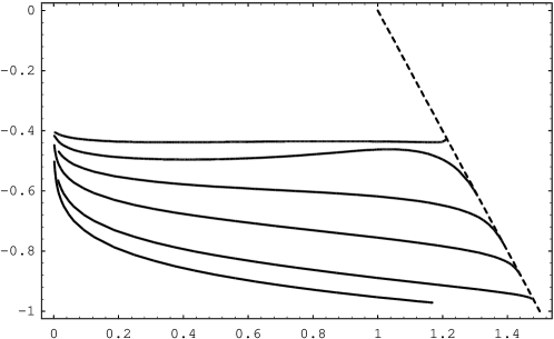
Figure 10: Curves in the $(\gamma,\eta)$-plane representing regular solutions for the case $d=3$, $n=4$, with $N=1$, 2, 5, 10, 20, 50. Curves lying higher correspond to larger values of $N$. The dashed line is $\eta=2-2\gamma$.

Within the accuracy of the computation it can be concluded that as $N$ grows the functions $\eta_{n}(\gamma)$, existing for $-\infty<\gamma<0$, transform to $\eta_{n}=$const, existing only for $\gamma_{*n}<\gamma<0$. The latter is the limit we expect from our studies of the case $N=\infty$ in Sect. 3.

5 Discussion and conclusions

We studied families of regular FP solutions of the Polchinski ERG equation for the $O(N)$-model in the LPA. The families are labeled by the integer $n\geq 1$ and are represented by curves $\eta_{n}(\gamma)$ in the $(\gamma,\eta)$-plane. We proved that for given $N$ the pattern of the curves is universal for all $d$ and described by Eq. (67).

There is a one-to-one correspondence between the curves for different $N$. In particular, for any $N$

$$\eta_{n}(0)=2-\frac{nd}{n+1},$$

see Eq.(71), and $\eta_{n}\rightarrow 2-d$ as $\gamma\rightarrow-\infty$ for $n$ odd. Further properties of the curves were discussed in detail in Sect. 4.

As $N$ increases the $\eta_{1}(\gamma)$ curve transforms into the corresponding curve for $N=\infty$. The rest of the curves transform into the straight lines given by Eq. (60).

For the $N=\infty$ case the solutions were studied analytically. We have shown that most of them have a singularity at some finite point (see Eq. (41)) and are not acceptable from the physical point of view. The condition of regularity imposes a relation between the parameters $\eta$ and $\gamma$. We analyzed this condition of regularity explicitly and demonstrated how various classes of FP solutions appear.

The analysis of the $N=\infty$ case, carried out in the article, gives an explicit analytical illustration of the condition which selects regular solutions. This enables to get an insight into the nature of FP solutions of the ERG equations in the LPA. Usually these equations are stiff, and gaining a better understanding of the behavior of its solutions is quite valuable.

We would like to mention that the pattern of the curves resembles the pattern of eigenvalues ($\eta_{n}$) of an eigenvalue problem with a parameter ($\gamma$). As the parameter varies the levels change and various phenomena, like level crossing, may occur.

The results can be extended to higher order approximations of the Polchinski ERG equation. In particular, as it was mentioned in the Introduction, the regular solutions studied here can be used as initial input in the iteration procedure used for solving the next-to-leading order approximation. Methods of the analysis and the obtained results can also be useful in studies of ERG equations of other types in scalar models, as well as in other classes of theories, in particular in fermionic theories.

References

• [1] K.G. Wilson, Phys. Rev.  B4, 3174, 3184 (1971); K.G. Wilson and J.B. Kogut, Phys. Rep.  C12, 75 (1974).
• [2] S. Ma, Rev. Mod. Phys.  45, 589 (1973).
• [3] F.J. Wegner and A. Houghton, Phys. Rev.  A8, 401 (1973).
• [4] S. Weinberg, in Understanding the Fundamental Constituents of Matter, Erice 1976, ed. A. Zichichi (Plenum Press, New York, 1978).
• [5] J. Polchinski, Nucl. Phys.  B231, 269 (1984).
• [6] A. Hasenfratz and P. Hasenfratz, Nucl. Phys.  B270, 687 (1986).
• [7] T.R. Morris, in New Developments in Quantum Field Theory, NATO ASI Series 366, (Plenum Press, New York, 1998), p. 147, hep-th/9709100; Prog. Theor. Phys. Suppl.  131, 395 (1998) [hep-th/9802039]; in The Exact Renormalization Group, ed. A. Krasnitz et al. (World Scientific, 1999), p. 1, hep-th/9810104.
• [8] Yu.A. Kubyshin, Int. J. Mod. Phys.  B12, 1321 (1998).
• [9] C. Bagnuls and C. Bervillier, Phys. Rep.  348, 91 (2001).
• [10] D.-U. Jungnickel and C. Wetterich, in The Exact Renormalization Group, ed. A. Krasnitz et al. (World Scientific, 1999), p. 41, hep-th/9710397; C. Wetterich, Int. J. Mod. Phys.  A16, 1951 (2001); J. Berger, N. Tetradis and C. Wetterich, Phys. Rep.  363, 233 (2002).
• [11] Yu.M. Ivanchenko and A.A. Lisyansky, Physics of Critical Phenomena (Springer, New York, 1995).
• [12] R.D. Ball and R.S. Thorne, Annals. Phys.  236, 117 (1994).
• [13] J.F. Nicoll and T.S. Chang, Phys. Lett.  A62, 287 (1977).
• [14] T.S. Chang, D.D. Vvedensky and J.F. Nicoll, Phys. Rep.  217, 279 (1992).
• [15] M. Bonini, M. D’Attanasio, and G. Marchesini, Nucl. Phys.  B409, 441 (1993).
• [16] C. Wetterich, Phys. Lett.  B301, 90 (1993).
• [17] T.R. Morris, Int. J. Mod. Phys.  A9, 2411 (1994).
• [18] J.I. Latorre and T.R. Morris, J. High Energy Phys.  0011, 004 (2000); Int. J. Mod. Phys.  A16, 2071 (2001); S. Arnone, A. Gatti and T.R. Morris, J. High Energy Phys.  0205, 059 (2002).
• [19] A. Margaritis, G. Ódor, and A. Patkós, Z. Phys.  C39, 109 (1988); M. Alford, Phys. Lett.  B336, 237 (1994).
• [20] R.J. Myerson, Phys. Rev.  B12, 2789 (1975).
• [21] G.R. Golner, Phys. Rev.  B33, 7863 (1986).
• [22] T.R. Morris, Phys. Lett.  B329, 241 (1994).
• [23] T.R. Morris, Phys. Lett.  B334, 355 (1994).
• [24] P.E. Haagensen, Yu.A. Kubyshin, J.I. Latorre and E. Moreno, Phys. Lett.  B323, 330 (1994); in Proceedings of the International Seminar ”Quarks-94”, ed. D.Yu. Grigoriev et al.  (World Scientific, 1995), p. 422, hep-th/9408050.
• [25] J.F. Nicoll, T.S. Chang and H.E. Stanley, Phys. Rev. Lett.  33, 540 (1974); Phys. Rev.  A13, 1251 (1976); V.I. Tokar, Phys. Lett.  A104, 135 (1984).
• [26] R.D. Ball, P.E. Haagensen, J.I. Latorre and E. Moreno, Phys. Lett.  B347, 80 (1995).
• [27] T.R. Morris, Phys. Lett.  B345, 139 (1995).
• [28] T.R. Morris, Nucl. Phys. Proc. Suppl.  42, 811 (1995); Nucl. Phys.  B458 [FS], 477 (1996); Phys. Rev. Lett.  77, 1658 (1996); Int. J. Mod. Phys.  B12, 1343 (1998); Nucl. Phys.  B495, 477 (1997).
• [29] J. Comellas and A. Travesset, Nucl. Phys.  B498, 539 (1997).
• [30] T.R. Morris and M.D. Turner, Nucl. Phys.  B509, 637 (1998); M. D’Attanasio and T.R. Morris, Phys. Lett.  B409, 363 (1997).
• [31] J. Comellas, Nucl. Phys.  B509, 662 (1998).
• [32] Yu.A. Kubyshin, R. Neves and R. Potting, in The Exact Renormalization Group, ed. A. Krasnitz et al. (World Scientific, 1999), p. 159, hep-th/981151.
• [33] Yu.A. Kubyshin, R. Neves and R. Potting, Int. J. Mod. Phys.  A16, 2065 (2001).
• [34] T.R. Morris and J.F. Tighe, J. High Energy Phys.  9908, 007 (1999); Int. J. Mod. Phys.  A16, 2095 (2001).
• [35] G. Felder, Comm. Math. Phys.  111, 101 (1987).
• [36] A.E. Filippov, Theor. Math. Phys.  91, 551 (1992); A.E. Filippov and S.A. Breus, Phys. Lett.  A158, 300 (1991); Physica A192, 486 (1993).
• [37] N. Tetradis and C. Wetterich, Nucl. Phys.  B422, 541 (1994).
• [38] J. Comellas, Yu.A. Kubyshin and E. Moreno, Nucl. Phys.  B490, 653 (1997).
• [39] T.R. Morris, Nucl. Phys.  B573, 97 (2000) [hep-th/9910058]; J. High Energy Phys.  0012, 012 (2000).
• [40] S. Ma, Phys. Lett.  A43, 479 (1973).
• [41] F. David, D.A. Kessler and H. Neuberger, Phys. Rev. Lett.  53, 2071 (1984); Nucl. Phys.  B257, 695 (1985).
• [42] J. Zinn-Justin, Quantum Field Theory and Critical Phenomena (Clarendon Press, Oxford, 1993); Phys. Rep.  344, 159 (2001).
• [43] G. Zumbach, Nucl. Phys.  B413, 754 (1994).
• [44] M. Reuter, N. Tetradis and C. Wetterich, Nucl. Phys.  B401, 567 (1993).
• [45] I.S. Gradshteyn and I.M. Ryzhik, Tables of Integrals, Series and Products: 6th Edition (Academic Press, San Diego, 2000).