Abstract

We present an exact normalisable zero-energy chiral fermion solution for abelian BPS dipoles. For a single dipole, this solution is contained within the high temperature limit of the SU(2) caloron with non-trivial holonomy.

1 The Dirac Monopole

A convenient representation for the Dirac monopole [1] is given by

$$\vec{A}=g\hat{n}\wedge\vec{\nabla}\log w(\vec{x}),\quad w(\vec{x})=|\vec{x}|+\vec{x}\cdot\hat{n},$$ (1)

where $w(\vec{x})$ is positive, but vanishes along the Dirac string pointing along $-\hat{n}$, as seen from the monopole. The magnetic field is

$$\vec{B}=\vec{\nabla}\wedge\vec{A}=-g\vec{\nabla}\left(\hat{n}\cdot\vec{\nabla}\log w(\vec{x})\right)+g\hat{n}\Delta\log w(\vec{x})=\vec{B}_{\rm reg}+\vec{B}_{\rm str},$$ (2)

and using that $\hat{n}\cdot\vec{\nabla}\log w(\vec{x})=1/|\vec{x}|$ (the derivative along the direction of the Dirac string) is independent of $\hat{n}$, the first term gives rise to the radial magnetic field associated with a magnetic point charge, whereas the second term represents the Dirac string, which takes care of the return flux. This follows from the fact that $\log w(\vec{x})$ is harmonic, except where $w(\vec{x})$ vanishes. To be specific, choosing for convenience $\hat{n}=\hat{e}_{3}=(0,0,1)$, we find $\vec{B}=g\vec{x}/|\vec{x}|^{3}+4\pi g\hat{e}_{3}\delta(x)\delta(y)\theta(-z)$ and $\vec{\nabla}\cdot\vec{B}_{\rm reg}=-\vec{\nabla}\cdot\vec{B}_{\rm str}=4\pi g\delta_{3}(\vec{x})$. It gives the appropriate magnetic point charge for $\vec{B}_{\rm reg}$, but when including the return flux $\vec{\nabla}\cdot\vec{B}=0$, as it should.

The function $\log w(\vec{x})$ can be viewed as a potential, although from the point of view of the Maxwell equations it is more natural to consider $A_{0}\equiv-g\hat{n}\cdot\nabla\log w(\vec{x})$ as such. Not only $\vec{B}_{\rm reg}=\vec{\nabla}A_{0}$, but also as the time component of the Euclidean vector potential this choice of $A_{0}$ gives rise to a self-dual configuration, with $\vec{E}=\vec{\nabla}A_{0}=\vec{B}_{\rm reg}$. The usefulness of $w(\vec{x})$ becomes clear when one considers the massless (Euclidean) Dirac equation in such a background. As usual we split this into positive and negative chirality Weyl equations,

$$H_{+}=\bar{D}=D^{\dagger}=-\bar{\sigma}^{\mu}D_{\mu},\quad H_{-}=D=\sigma^{\mu}D_{\mu},$$ (3)

where $D_{\mu}=\partial_{\mu}+ieA_{\mu}$ is the covariant derivative and $\sigma_{j}=i\tau_{j}$, whereas $\sigma_{0}$ is the $2\times 2$ identity matrix. For $\hat{n}=\hat{e}_{3}$ a solution of $\bar{D}\Psi=0$ is given by

$$\Psi(\vec{x})=\sqrt{w(\vec{x})}\pmatrix{-\partial_{1}+i\partial_{2}\cr\partial_{3}\cr}\log w(\vec{x}).$$ (4)

If so desired a (spin-)rotation allows one to obtain the solution for arbitrary $\hat{n}$, but to keep things simple we stick to $\hat{n}=\hat{e}_{3}$, such that

$$-iH_{+}=\pmatrix{\partial_{3}+i\partial_{0}&\hphantom{-}\partial_{1}-i\partial_{2}\cr\partial_{1}+i\partial_{2}&-\partial_{3}+i\partial_{0}\cr}-eg\pmatrix{-\partial_{3}&-\partial_{1}+i\partial_{2}\cr\partial_{1}+i\partial_{2}&-\partial_{3}\cr}\log w(\vec{x}).$$ (5)

Using the Dirac quantisation condition $eg={\scriptstyle{{1\over 2}}}$, one easily verifies

$$-iH_{+}\Psi(\vec{x})=\sqrt{w(\vec{x})}\pmatrix{0\cr-\Delta\log w(\vec{x})\cr}.$$ (6)

Since $\sqrt{w}$ vanishes along the Dirac string, we find that $\sqrt{w}\Delta\log w=0$ (as a distribution), hence $\bar{D}\Psi=0$. Likewise $|\Psi|^{2}=w\vec{\nabla}\log w\cdot\vec{\nabla}\log w=\Delta w-w\Delta\log w$. Thus $|\Psi|^{2}=\Delta w=2/|\vec{x}|$ has an integrable singularity at the origin, and the Dirac string is invisible, as it should. Nevertheless, $\Psi$ does not decay sufficiently fast to be normalisable. Note that the zero-mode is time independent. Putting $\partial_{0}$ to zero, $H$ is precisely the Dirac Hamiltonian, with $A_{0}$ playing the role of a Higgs field. A non-zero asymptotic value of $A_{0}$ would lead to a mass scale and exponentially decaying wave functions.

It should not come as a surprise that existence of zero-energy solutions is sensitive to the sign of the electron charge (relative to $g$). With $eg=-{\scriptstyle{{1\over 2}}}$ we have

$$-iH_{+}\left(\frac{1}{\sqrt{w(\vec{x})}}\pmatrix{\partial_{3}\cr\partial_{1}+i\partial_{2}\cr}\log w(\vec{x})\right)=\frac{1}{\sqrt{w(\vec{x})}}\pmatrix{\Delta\log w(\vec{x})\cr 0\cr}.$$ (7)

However, here the singularity of the Dirac string is no longer nullified but enhanced. Nevertheless, it can be turned into a proper zero-energy solution, identical to $\Psi^{\dagger}\sigma_{2}$, by replacing $w(\vec{x})$ with $1/w(\vec{x})$, but this has the same effect as changing $g$ to $-g$, explaining why the new zero-energy solution is the charge conjugate of $\Psi$ in Eq. (4). Negative chirality zero-energy solutions cannot appear because the self-duality of $A_{\mu}$ implies that $\bar{D}D=-D_{\mu}^{2}$. Therefore such a solution would satisfy $D_{\mu}\Psi=0$, which is ruled out.

It is well known that the ’t Hooft-Polyakov monopole [2] allows for a normalisable chiral zero-energy solution of the Dirac equation [3]. The size of the core of these non-abelian monopoles is determined by the mass scale set by the asymptotic value of the Higgs field. When the core size shrinks to zero, so does the support for the zero-mode. Adding to the Higgs field $\Phi={\scriptstyle{{1\over 2}}}\Phi^{a}\sigma_{a}$ a constant element in U(1), $\Phi_{z}=\Phi-2\pi iz$, as it appears in Nahm’s work [4], the zero-mode remains normalisable for a finite range of $z$ determined by the Callias index theorem [5]. Our solution corresponds to $z$ at the boundary of this range, where the zero-mode fails to be normalisable. This boundary value of $z$ is defined by $\det(\Phi_{z})=0$, and the abelian field $A_{0}$ given above corresponds to the isospin component of $\Phi_{z}$ responsible for this vanishing eigenvalue. It does imply the support of the zero-mode is no longer confined to the non-abelian core.

There has been another context in which solutions to the Dirac equation in the background of a monopole have appeared in the past, namely that of monopole-induced proton decay (the Callan-Rubakov effect [6]). Boundary conditions [7] for the fermions are imposed at the core of the monopole to describe the scattering states in the limit where the size of the monopole core can be neglected, so as to properly reflect the breaking of B-L, compatible with the chiral anomaly. There it is assumed, as for the Jackiw-Rebbi zero-energy solution, that the Higgs field approaches a non-zero constant at infinity, which through the Yukawa coupling gives a mass to the fermions. In our case the asymptotic value of the Higgs field ($A_{0}$) vanishes and as we will see, the limit of zero monopole core size can be taken without any approximation, but at the expense of the zero-energy state being non-normalisable.

2 The Abelian BPS Dipole

To find a normalisable zero-energy solution, we have to do something about the asymptotic behaviour. A natural way to achieve this is to consider an abelian BPS (self-dual) dipole, or bipole for short. We now profit from having expressed the zero-mode in terms of the function $w$. The bipole field is generated by

$$\log w(\vec{x})=\log(|\vec{x}|+\vec{x}\cdot\hat{n})-\log(|\vec{x}+s\hat{n}|+\vec{x}\cdot\hat{n}+s)$$ (8)

where the first term represents a monopole at $\vec{x}=\vec{0}$ and the second term, with the opposite sign, an anti-monopole at $\vec{x}=-s\hat{n}$. It is convenient to express $w(\vec{x})$ as

$$w(\vec{x})=\frac{r_{1}+r_{2}-s}{r_{1}+r_{2}+s},$$ (9)

where $\vec{r}_{1}=\vec{x}$ and $\vec{r}_{2}=\vec{x}+s\hat{n}$. This shows that the Dirac strings of the monopole and anti-monopole partly cancel. All that we need to check is if $\Psi$, with this choice of $w$ is now normalisable. A simple computation shows that $|\Psi(\vec{x})|^{2}=\Delta w(\vec{x})=\frac{4s^{2}}{r_{1}r_{2}(r_{1}+r_{2}+s)^{2}}$, as shown in Fig. 1 (left). This is indeed integrable at the location of the two point charges and at infinity, $\int d^{3}x|\Psi(\vec{x})|^{2}=\int d^{3}x\Delta w(\vec{x})=4\pi s$, using that $w(\vec{x})=1-s/|\vec{x}|+{\cal{O}}(1/|\vec{x}|^{3})$.

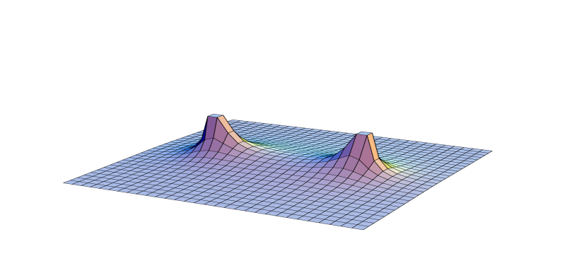
Figure 1.  : The chiral zero-mode for the bipole of charge $k=1$ (left) and $k=2$ (right). Plotted is $|\Psi(\vec{x})|^{2}$, the integral normalised to 1, as a function of $\sqrt{x^{2}+y^{2}}$ and $z$ on a linear scale for $s=.5$, cutoff at respectively $|\Psi|^{2}=5$ (left) and .5 (right).

Having found a normalisable zero-mode for one bipole, a generalisation to a collection of bipoles is obvious, by taking the product of $w(\vec{x})$ for each such bipole. This does not affect the property that $w(\vec{x})$ is positive, vanishes along the Dirac strings, and its logarithm is harmonic elsewhere. However, the form of the zero-mode requires all factors $w$ to be formulated in terms of the same $\hat{n}$, which means all bipoles have to point in the same direction, i.e. the magnetic moments of all bipoles have to be uni-directional. It is not clear if this is just a limitation of our simple ansatz. For multi-bipoles, all separated much further than each of the individual bipole sizes ($s$), $|\Psi|^{2}$ will near each bipole be of the same form as for a single bipole. However, when two or more bipoles coincide, or equivalently when $g$ is bigger than the minimal Dirac value of $\frac{1}{2e}$, $|\Psi|^{2}$ will be suppressed along the line segment connecting the two charges. To demonstrate this, we note that for $g=\frac{k}{2e}$, $w_{k}(\vec{x})=w^{k}(\vec{x})$, with $w(\vec{x})$ as given in Eq. (9). Thus, using $w(\vec{x})\Delta\log w(\vec{x})=0$, we find

$$|\Psi(\vec{x})|^{2}=\Delta w(\vec{x})^{k}=k^{2}w^{k-1}(\vec{x})\Delta w(\vec{x})=\frac{4s^{2}k^{2}(r_{1}+r_{2}-s)^{k-1}}{r_{1}r_{2}(r_{1}+r_{2}+s)^{k+1}},$$ (10)

which integrates to $4\pi ks$. The case for $k=2$ is shown in Fig. 1 (right).

3 The Caloron

The context in which the bipole appears in a natural way is the caloron with non-trivial holonomy [9], in the infinite temperature limit. The periodic boundary conditions in the Euclidean time direction, relevant for these finite temperature instantons, allow for a non-trivial holonomy determined by the Polyakov loop, which approaches a constant value at spatial infinity,

$${{\cal P}_{\infty}}=\lim_{|\vec{x}|\rightarrow\infty}P(\vec{x}),\quad P(\vec{x})={\rm P}\exp(\int_{0}^{\beta}A_{0}(t,\vec{x})dt).$$ (11)

With $A_{0}$ playing the role of a Higgs field, a non-trivial value implies that an SU($n$) charge one caloron splits into $n$ constituent BPS monopoles, whose masses are determined by the eigenvalues of the Polyakov loop

$${{\cal P}_{\infty}^{0}}\equiv\exp(2\pi i\mbox{diag}(\mu_{1},\mu_{2},\cdots,\mu_{n})),\quad\sum_{i=1}^{n}\mu_{i}=0.$$ (12)

arranged to satisfy $\mu_{1}\leq\cdots\mu_{n}\leq\mu_{n+1}\equiv\mu_{1}+1$. The constituent masses $8\pi^{2}\nu_{m}$, with $\nu_{m}\equiv(\mu_{m+1}-\mu_{m})/\beta$, add up to $8\pi^{2}/\beta$ such that the action equals that of a charge one instanton. The presence of these constituents is easily established from the formula [9, 10]

$${\rm Tr}F_{\alpha\gamma}^{\,2}(x)=\partial_{\alpha}^{2}\partial_{\gamma}^{2}\log\psi(x),\quad\psi(x)={\scriptstyle{{1\over 2}}}{\rm tr}({\cal{A}}_{n}\cdots{\cal{A}}_{1})-\cos(2\pi t),$$ (13)

$${\cal{A}}_{m}\equiv\frac{1}{r_{m}}\left(\!\!\!\begin{array}[]{cc}r_{m}\!\!&|\vec{\rho}_{m+1}|\\ 0\!\!&r_{m+1}\end{array}\!\!\!\right)\left(\!\!\!\begin{array}[]{cc}\cosh(2\pi\nu_{m}r_{m})\!\!&\sinh(2\pi\nu_{m}r_{m})\\ \sinh(2\pi\nu_{m}r_{m})\!\!&\cosh(2\pi\nu_{m}r_{m})\end{array}\!\!\!\right),$$ (18)

where we introduced $r_{m}\equiv|\vec{x}-\vec{y}_{m}|$ and $\vec{\rho}_{m}\equiv\vec{y}_{m}-\vec{y}_{m-1}$ ($r_{n+1}\equiv r_{1}$ and $\vec{y}_{n+1}\equiv\vec{y}_{1}$), with $\vec{y}_{m}$ the location of the $m^{\rm th}$ constituent monopole with a mass $8\pi^{2}\nu_{m}$.

The basic ingredient in the construction of caloron solutions is the Greens function $\hat{f}_{x}$ defined on the circle, $z\in[0,\beta^{-1}]$, satisfying [9, 10]

$$\left(\left(\frac{1}{2\pi i}\frac{d}{dz}-t\right)^{2}+r^{2}(\vec{x};z)+\frac{1}{2\pi}\sum_{m}\delta(z-\mu_{m}/\beta)|\vec{\rho}_{m}|\right)\hat{f}_{x}(z,z^{\prime})=\delta(z\!-\!z^{\prime}),$$ (19)

where $r^{2}(\vec{x};z)\!=\!r_{m}^{2}$ for $z\in[\mu_{m}/\beta,\mu_{m+1}/\beta]$. The variable $z$ can be introduced through Fourier transformation with respect to time, where the Fourier coefficients are related to the ADHM data [11] of instantons, periodic up to a gauge rotation with ${{\cal P}_{\infty}}$ (giving the solution in the so-called algebraic gauge). This is in one-to-one relation with the Nahm transformation [12]. For $\mu_{m}/\beta\leq z^{\prime}\leq z\leq\mu_{m+1}/\beta$ ($\hat{f}_{x}(z^{\prime},z)=\hat{f}_{x}^{*}(z,z^{\prime})$ for $z<z^{\prime}$) the explicit result [9, 13] for the Greens function can be expressed as

$$\hat{f}_{x}(z,z^{\prime})=\frac{\pi e^{2\pi it(z-z^{\prime})}}{r_{m}\psi}\langle v_{m}(z^{\prime})|{\cal{A}}_{m\!-\!1}\cdots{\cal{A}}_{1}{\cal{A}}_{n}\cdots{\cal{A}}_{m}-e^{-2\pi it}|\sigma_{2}v_{m}(z)\rangle,$$ (20)

where the spinor $v_{m}(z)$ is defined by

$$v_{m}(z)=\pmatrix{\sinh[2\pi(z-\mu_{m}/\beta)r_{m}]\cr\cosh[2\pi(z-\mu_{m}/\beta)r_{m}]\cr}.$$ (21)

The chiral Dirac, or Weyl equation can be solved with the boundary condition $\Psi_{z}(t+\beta,\vec{x})=\exp(2\pi iz\beta){{\cal P}_{\infty}}\Psi_{z}(t,\vec{x})$ (in addition to the two component spinor index, there is now also a colour index). With $z={\scriptstyle{{1\over 2}}}\beta^{-1}$ one obtains the finite temperature “anti-periodic” fermion zero-mode, and for $z=0$ the “periodic” zero-mode.

To be specific, for the SU(2) caloron we have $\mu_{2}=-\mu_{1}\equiv\beta\omega$ and $|\vec{\rho}_{1}|=|\vec{\rho}_{2}|\equiv\pi\rho^{2}/\beta$ ($\rho$ is the instanton scale parameter). The gauge field and zero-mode can be expressed in terms of the functions $\phi^{-1}\equiv 1-\rho^{2}\hat{f}_{x}(\omega,\omega)/\beta$ and $\chi\equiv\rho^{2}\hat{f}_{x}(\omega,-\omega)/\beta$. In the algebraic gauge, choosing ${{\cal P}_{\infty}}={{\cal P}_{\infty}^{0}}$ and the constituents along the $z$-axis (by proper combinations of gauge and space rotations this can always be achieved) [9]

$$A_{\alpha}=\frac{i}{2}\bar{\eta}^{3}_{\alpha\gamma}\tau_{3}\partial_{\gamma}\log\phi+\frac{i}{2}\phi{\rm Re}\left((\bar{\eta}^{1}_{\alpha\gamma}-i\bar{\eta}^{2}_{\alpha\gamma})(\tau_{1}+i\tau_{2})\partial_{\gamma}\chi\right),$$ (22)

with $\bar{\eta}_{\alpha\gamma}^{a}\sigma_{a}\equiv\bar{\sigma}_{[\alpha}\sigma_{\gamma]}$ the anti-selfdual ’t Hooft tensor, and [14]

$$\Psi_{z}(x)=\frac{\rho}{2\pi\beta}\sqrt{\phi(x)}\left(\pmatrix{\partial_{2}+i\partial_{1}\cr\partial_{0}-i\partial_{3}\cr}\hat{f}_{x}(\omega,z),~{}\pmatrix{-\partial_{0}-i\partial_{3}\cr\hphantom{-}\partial_{2}-i\partial_{1}\cr}\hat{f}_{x}(-\omega,z)\right).$$ (23)

Particularly simple and valid for arbitrary SU($n$), is the expression for the density of the fermion zero-modes [13, 14]

$$|\Psi_{z}(x)|^{2}=-(4\pi^{2}\beta)^{-1}\partial_{\alpha}^{2}\hat{f}_{x}(z,z).$$ (24)

The limit $\beta\rightarrow 0$ can be seen as a dimensional reduction and only the time independent field components are expected to survive in this high temperature limit. It is therefore more appropriate to consider the periodic gauge. For general $z$ this periodic gauge is obtained by applying the gauge transformation $g(t)\equiv e^{-tA_{0}^{\infty}}$, where $A_{\alpha}^{\infty}\equiv 2\pi i(\omega\tau_{3}-z)\delta_{\alpha 0}$, such that $\tilde{\Psi}_{z}=g(t)\Psi_{z}$ and the new gauge field $\tilde{A}$ are now periodic, with

$$\tilde{A}_{\alpha}=A_{\alpha}^{\infty}+\frac{i}{2}\bar{\eta}^{3}_{\alpha\gamma}\tau_{3}\partial_{\gamma}\log\phi+\frac{i}{2}\phi{\rm Re}\left((\bar{\eta}^{1}_{\alpha\gamma}-i\bar{\eta}^{2}_{\alpha\gamma})(\tau_{1}+i\tau_{2})e^{-2\pi it\nu_{1}}\partial_{\gamma}\chi\right),$$ (25)

We find that [9] $\lim_{\beta\rightarrow 0}\chi(x)=0$ and $\lim_{\beta\rightarrow 0}\phi^{-1}(x)=w(\vec{x})$ with $w(\vec{x})$ as in Eq. (9). The resulting abelian gauge field splits into an isospin up and down component, decoupled in the Weyl equation. For $z=0$ this gives a mass of $\pi\nu_{1}$ to both isospin components, which contribute equally to the density, and the zero-mode is supported entirely at $\vec{y}_{1}$, whereas for $z={\scriptstyle{{1\over 2}}}\beta^{-1}$ the mass is $\pi\nu_{2}$, but the zero-mode is now supported entirely at $\vec{y}_{2}$. For other values of $z$ the mass will depend on the isospin component, but as long as $z\neq\pm\omega$ the zero-mode remains localised to either of the two constituent locations, jumping from one to the other when $z$ crosses $\pm\omega$, where the zero-mode becomes delocalised, having support at both constituents simultaneously. Indeed, for $z=\omega$

$$\Psi_{\omega}(x)=\frac{\sqrt{\phi(x)}}{2\pi\rho}\left(\frac{1}{\phi(x)}\pmatrix{\partial_{2}+i\partial_{1}\cr\partial_{0}-i\partial_{3}\cr}\log\phi(x),~{}\pmatrix{-\partial_{0}-i\partial_{3}\cr\hphantom{-}\partial_{2}-i\partial_{1}\cr}\chi^{*}(x)\right),$$ (26)

whereas for $z=-\omega$, the same result follows after charge and isospin conjugation, $\Psi^{1}_{-\omega}(x)=-\Psi^{2}_{\omega}(x)^{\dagger}\sigma_{2}$ and $\Psi^{2}_{-\omega}(x)=\Psi^{1}_{\omega}(x)^{\dagger}\sigma_{2}$ (with the isospin index made explicit). Since $\chi$ vanishes in the high temperature limit, the only surviving isospin component of the Weyl zero-mode is the one for which the asymptotic value of $A_{0}$ vanishes, and for which the zero-mode is time independent. This non-trivial isospin component agrees (up to an irrelevant factor $-2\pi i\rho$) with Eq. (4), for $w(\vec{x})=\phi^{-1}(x)$.

For the high temperature limit to be smooth and unambiguous, it was essential that $\phi$ be time independent, $\phi^{-1}\Delta\log\phi=0$, and that $\chi=0$. It is interesting to note that, imposing self-duality on Eq. (22), leads to a natural generalisation at finite temperature

$$\phi^{-2}\partial_{\alpha}^{2}\log\phi+|(\partial_{1}-i\partial_{2})\chi|^{2}+|(\partial_{0}-i\partial_{3})\chi|^{2}=0,$$ (27)

$$\phi^{-1}(\partial_{1}+i\partial_{2})\phi^{2}(\partial_{1}-i\partial_{2})\chi+\phi^{-1}(\partial_{0}+i\partial_{3})\phi^{2}(\partial_{0}-i\partial_{3})\chi=0.$$

In principle, but not in practise, this can be used to define $\phi$ and $\chi$. Interestingly these equations also appear when formulating self-duality in the so-called R-gauge introduced by Yang [15], after a suitable Bäcklund transformation [16].

We will end with a few words on the case of SU($n>2$). In the high temperature limit the zero-mode is again exponentially localised at one of the constituents [13]. This we can read off from Eq. (24), using the explicit expression for $\hat{f}_{x}(z,z)$ given in Eq. (20). When $z$ passes through $\mu_{m}/\beta$ the zero-mode jumps from one constituent location to the other, and only for these values of $z$ the zero-mode will delocalise, with the proviso that it will only “see” two out of the $n$ constituents. In the periodic gauge, diagonalising $A_{0}$ at infinity by a constant gauge rotation, we have $A_{0}\rightarrow 2\pi i\mbox{diag}(\mu_{1}/\beta-z,\mu_{2}/\beta-z,\cdots,\mu_{n}/\beta-z)$. The only non-vanishing colour component of the fermion zero-mode is the one for which $\mu_{j}/\beta-z=0$. The resulting configuration is again that of the bipole in section 2.

4 Discussion

An interesting question is if there is some physical significance to the zero-modes, like for chiral symmetry breaking in the effective description of QCD in terms of monopoles obtained through abelian projection [17]. But first we would like to better understand how to go beyond the case where the magnetic moments of the bipoles are no longer parallel. A natural setting in which to address this particular question would be through the study of charge $k>1$ calorons. It is not clear if in the high temperature limit a global abelian embedding for the case of non-parallel magnetic moments exists. Even when the magnetic moments are parallel, one would expect $k$ independent zero-energy solutions, of which we have only provided one.

What led us to the results presented in this paper, was an attempt to solve the Weyl equation in the background of the abelian gauge field [18] that is obtained from the Nahm transformation of an SU(2) charge one instanton on $T^{3}\times R$. This self-dual abelian gauge field is described by two bipoles on $T^{3}$, but unfortunately with anti-parallel orientations. Furthermore, two zero-modes are required in order for the (inverse) Nahm transformation to reconstruct the SU(2) instanton, for which $z$ is to be identified with the time. When the zero-modes are localised at the monopole singularities, it can be shown that the resulting SU(2) gauge field is abelian. This describes the asymptotically flat connections ($F=0$) of the instanton on $T^{3}\times R$, required for the integral over the action density to be finite, and equal to $8\pi^{2}$. Thus, to obtain genuine non-abelian behaviour the zero-mode has to become delocalised for certain values of $z$. Here the gauge field is no longer flat ($F\neq 0$) and the density will have a maximum, in accordance with a general relationship between holonomies (with respect to each of the generating circles of the manifold) of a self-dual gauge field on the one hand and the constituent locations of the Nahm dual gauge field on the other hand. This dual relationship has been verified in a careful numerical study [19]. Similar results have been seen [20] for instantons on $T^{2}\times R^{2}$.

It is the applications to the Nahm transformation on a torus that has been our prime motivation for studying this problem. Taken out of this context and the context of the caloron, our exact result for the chiral zero-mode is so simple we believe it is worthwhile to share it with the reader.

References

- [1] P.A.M. Dirac, Proc. Roy. Soc. A133 (1931) 60.
-
[2]
G. ’t Hooft, Nucl. Phys. Nucl. Phys. B79 (1974) 194;
A.M. Polyakov, JETP Lett. 20 (1974) 194. - [3] R. Jackiw and C. Rebbi, Phys. Rev. D13 (1976) 3398.
- [4] W. Nahm, Phys. Lett. B90 (1980) 413.
-
[5]
C. Callias, Comm. Math. Phys. 62 (1978) 213;
R. Bott and R. Seeley, Comm. Math. Phys. 62 (1978) 235. -
[6]
V.A. Rubakov, JETP Lett. 33 (1981) 644;
Nucl. Phys. B203 (1982) 311;
C.G. Callan, Phys. Rev. D25 (1982) 2142; Phys. Rev. D26 (1982) 2058. -
[7]
Y. Kazama, C.N. Yang and A.S. Goldhaber,
Phys. Rev. D15 (1977) 2287;
A.S. Goldhaber, Phys. Rev. D16 (1977) 1815. -
[8]
E.B. Bogomol’ny, Sov. J. Nucl. Phys. 24 (1976) 449;
M.K. Prasad and C.M. Sommerfield, Phys. Rev. Lett. 35 (1975) 760. - [9] T.C. Kraan and P. van Baal, Nucl. Phys. B533 (1998) 627 [hep-th/9805168].
- [10] T.C. Kraan and P. van Baal, Phys. Lett. B435 (1998) 389 [hep-th/9806034].
- [11] M.F. Atiyah, N.J. Hitchin, V. Drinfeld and Yu.I. Manin, Phys. Lett. 65A (1978) 185.
- [12] W. Nahm, Self-dual monopoles and calorons, in: Lecture Notes in Physics 201 (1984) 189.
- [13] M.N. Chernodub, T.C. Kraan and P. van Baal, Nucl. Phys. B(Proc.Suppl.)83-84 (2000) 556 [hep-lat/9907001].
- [14] M. García Pérez, A. González-Arroyo, C. Pena and P. van Baal, Phys. Rev. D60 (1999) 031901 [hep-th/9905016].
- [15] C.N. Yang, Phys. Rev. Lett. 38 (1977) 1377.
- [16] M.K. Prasad, A. Sinha and Ling-Lie Chau Wang, Phys. Rev. D23 (1981) 2321.
- [17] G. ’t Hooft, Nucl. Phys. B190 [FS3] (1981) 455; Physica Scripta 25 (1982) 133.
- [18] P. van Baal, Phys. Lett. B448 (1999) 26 [hep-th/9811112].
- [19] M. García Pérez, A. González-Arroyo, C. Pena and P. van Baal, Nucl. Phys. B564 (1999) 159 [hep-th/9905138].
- [20] C. Ford, J.M. Pawlowski, T. Tok and A. Wipf, Nucl. Phys. B596 (2001) 387 [hep-th/0005221]; C. Ford and J.M. Pawlowski, to appear.