Star Algebra Projectors

Davide Gaiotto^a, Leonardo Rastelli^a, Ashoke Sen^b and Barton Zwiebach^c

 ^aDepartment of Physics

Princeton University, Princeton, NJ 08544, USA

E-mail: dgaiotto@princeton.edu, rastelli@feynman.princeton.edu

 ^bHarish-Chandra Research Institute

Chhatnag Road, Jhusi, Allahabad 211019, INDIA

and

Department of Physics, Penn State University

University Park, PA 16802, USA

E-mail: asen@thwgs.cern.ch, sen@mri.ernet.in

^cCenter for Theoretical Physics

Massachussetts Institute of Technology,

Cambridge, MA 02139, USA

E-mail: zwiebach@mitlns.mit.edu

Abstract

Surface states are open string field configurations which arise from Riemann surfaces with a boundary and form a subalgebra of the star algebra. We find that a general class of star algebra projectors arise from surface states where the open string midpoint reaches the boundary of the surface. The projector property of the state and the split nature of its wave-functional arise because of a nontrivial feature of conformal maps of nearly degenerate surfaces. Moreover, all such projectors are invariant under constant and opposite translations of their half-strings. We show that the half-string states associated to these projectors are themselves surface states. In addition to the sliver, we identify other interesting projectors. These include a butterfly state, which is the tensor product of half-string vacua, and a nothing state, where the Riemann surface collapses.

1 Introduction and Summary

The elucidation of tachyon dynamics and D-brane instabilities in string theory [1] has led to renewed investigations in open string field theory (OSFT). In particular, the star-algebra of open string fields, an associative multiplication introduced in [2], is the key algebraic structure in this theory. Recently, a formulation of open string field theory based on the tachyon vacuum – vacuum string field theory (VSFT) – was proposed in [3, 4] and investigated in [5]–[31]. In this theory, D-brane solutions were seen to correspond to open string fields that were projectors of the star algebra, i.e. elements which square to themselves, at least in the matter sector [5]. With the ghost structure of VSFT determined in [4, 14, 27], D-brane solutions are indeed seen to correspond strictly to projectors in the star algebra whose underlying conformal field theory (CFT) involves a twisting of the reparametrization ghost CFT [4]. Since no direct derivation of VSFT from conventional OSFT has yet been given, one must still consider VSFT somewhat conjectural. In fact, the present version of VSFT, where the kinetic operator is a ghost insertion with infinite strength at the open string midpoint, appears to be an extremely simple but somewhat singular limit that arises from a reparametrization that maps the open string to its midpoint [4]. We nevertheless expect that the connection between projectors of the star algebra and classical solutions of string field theory is a key property that will persist in other formulations of vacuum string field theory.

One is therefore led to investigate the existence of projectors of the star algebra of open string fields. For many years, the only string field known to multiply to itself was the identity string field. In fact, there were heuristic reasons to believe that projectors should be scarce in the star algebra. One can understand the difficulty in constructing projectors within the large class of field configurations that arise from path integration over fixed Riemann surfaces whose boundary consists of a parametrized open string and a piece with open string boundary conditions. Such string fields, called surface states, are easily star multiplied. One glues the right-half of the open string in the first surface to the left-half of the open string in the second surface, and the surface state corresponding to the glued surface is the desired product. It is clear from this description that multiplication of a surface state to itself leads to a surface state that looks different from the initial state. This is the reason why it seemed difficult, in general, to find projectors.

Leaving aside the identity string field, the first projector of the star algebra to be found was the sliver state [32, 33, 5]. It circumvents the above mentioned difficulty in an interesting way. Consider wedge states, surface states where the Riemann surface is an angular sector of the unit disk, with the left-half and the right-half of the open string being the two radial segments, and the unit radius arc having the open string boundary conditions. A wedge state is thus defined by the angle at the open string midpoint, and this angle simply adds under star multiplication, as is readily verified using the gluing prescription. The identity string field is the wedge state of zero angle, and the sliver is the wedge state of infinite angle! The addition of infinity to infinity is still infinity, and the sliver does star multiply to itself.

The sliver state was later recognized to be a string wave-functional that is split: it is the product of a functional of the left-half of the string times the same functional of the right-half of the open string. From this viewpoint, however, it seemed surprising that projectors would be hard to find: any symmetric split string wave-functional could serve as a projector. At least algebraically other projectors could easily be constructed by transforming the sliver by the action of star conjugation. Geometrically, however, it was not clear if there are other projectors which could be simply interpreted as other surface states.

In this paper we find large classes of projectors that indeed arise as surface states, and we explain the general mechanism by which they all evade the heuristic argument sketched earlier. All the projectors we find correspond to surface states where in the Riemann surface, the open string midpoint reaches the boundary where the open string boundary conditions are imposed (this is also the case for the sliver). The general situation is illustrated in figure 1. The vertical boundary is the open string, and its midpoint is indicated by a heavy dot. The rest of the boundary has open string boundary condition. More precisely, one can regulate the surface state by letting the open string midpoint reach the boundary when the regulator is removed. We explain that in the limit as the regulator is removed, the string wave-functional splits into a product of functionals. In considering the projector property, we examine the gluing of two regulated projector surface states. The gluing of the two regulated surfaces does not give a surface that looks like the original one, but rather, a surface that looks like the original one plus a short neck connecting it to an additional disk. We will explain that, conformally speaking, the short neck and the extra disk are in fact negligible perturbations in the sense that the resulting surface is accurately conformally equivalent to the original one without the extra disk. The agreement becomes exact as the regulator is removed. We consider this a key insight in the present paper. It shows how conformal equivalence is subtle enough to circumvent the heuristic arguments against the existence of projectors.

Figure 1: The generic kind of surface state providing a projector of the star algebra. The open string is the vertical boundary, and the open string midpoint is shown with a heavy dot. The rest of the boundary has open string boundary condition. Note that this part of the boundary touches the open string midpoint.

All the above are rank one projectors, and are expected to be related by star conjugation. Nevertheless there are special projectors that deserve special attention, for they satisfy a number of unusual conditions that may be of some relevance. In addition to the sliver, our studies have uncovered two special projectors – the butterfly and the ‘nothing’ state. We now summarize the special properties of these three projectors.

For the sliver $|\Xi\rangle$ we have:

• It is the projector that arises by repeated star multiplication of the SL(2,R) vacuum, namely $|\Xi\rangle=\lim_{n\to\infty}(|0\rangle)^{n}$.

• It is a projector whose Neumann matrix in the oscillator representation commutes with those defining the star product.

• It is the limit element of a sequence of surface states, the wedge states, defining an abelian subalgebra of the star algebra. The sliver state is annihilated by the star algebra derivation $K_{1}=L_{1}+L_{-1}$.

The properties of the “butterfly” state were announced in [4]:

• It has an extremely simple presentation in the Virasoro basis. It is just $\exp(-{1\over 2}L_{-2})|0\rangle$. It is annihilated by the star derivation $K_{2}=L_{2}-L_{-2}$.

• Its wave-functional is the product of vacuum wave-functionals for the left-half and the right-half of the string. Thus, it is the simplest projector from the viewpoint of half-strings.

• This is the state that appears to arise when considering the projector equations in the level expansion.

We constructed a family of projectors, all of them generalized butterflies, that interpolate from the sliver to the above canonical butterfly. The family can be continued beyond this canonical butterfly state up to a projector that we call the “nothing state”. The nothing state has the following properties:

• As we reach this state the Riemann surface becomes vanishingly small.

• It is annihilated by all the derivations $K_{2n}=L_{2n}-L_{-2n}$.

• It has a constant wave-functional.

Our general discussion shows that the condition that the open string midpoint touches the boundary ensures that projectors have split wave-functionals, that is, wave-functionals that factorize into a product of functionals each involving a half-string. We also show that the half-string states associated to surface state projectors are themselves surface states defined with the same boundary condition as the original projector, and give an explicit algorithm for the construction of such half-string states (see (4.14) and (4.15)). For example, our construction explains why the butterfly is the state corresponding to the tensor product of half string vacua with Neumann boundary condition at both ends if the original butterfly is defined with Neumann boundary condition. We believe this is an interesting insight into half-string formalisms, where boundary conditions at the string midpoint are subject to debate, and little geometrical understanding is available. We also point out a subtletly. When we say that a surface state is defined using a boundary condition, this means that the functional integral defining the state is done imposing the boundary condition in question along the boundary of the surface. A surface state $|\Sigma\rangle$ defined using a given boundary condition, say of Neumann type, may not necessarily satisfy this condition, namely, expectation values of the operator $\partial_{\sigma}X(\sigma)$ on the state $|\Sigma\rangle$ may not necessarily vanish at $\sigma=0,\pi$. This may happen when the boundary of the surface $\Sigma$ has a corner type singularity at the string endpoints. While such corner type singularities are not common in familiar surface states, they are generic for half-string states. Thus, for example, we find that unlike the canonical butterfly half-string state, the nothing half-string state satisfies a Dirichlet boundary condition at the point corresponding to the full string midpoint.

We also show that, just as for the sliver [34], all projectors defined with Neumann boundary condition have wave-functionals invariant under constant and opposite translations of the half-strings. This implies that the Neumann matrices associated to projectors all have a common eigenvector, the $\kappa=0$ eigenvector of $K_{1}$. This simply follows, as we explain in the text, because the associated half-string surface states carry no momentum.

This paper is organized as follows. We begin in section 2 by reviewing various geometrical presentations of surface states, and various concrete algebraic representations of the states. Section 3 is devoted to a discussion of some properties of conformal maps and conformal field theories which we use in later analysis. In particular we discuss factorization properties of conformal field theory correlators on a pinched disk that is about to split into two disconnected disks. Although we do not attempt to state precisely the way in which the surface must be pinched to achieve the desired factorization property, we state a conjecture that we expect to hold, and would guarantee the key properties. We also illustrate the conjecture with an example.

In section 4 we explain in general terms our understanding of the construction of split wave-functionals. In particular we argue, based on the results of sections 2, 3 that the surface state associated with a conformal map that sends the string midpoint to a point on the boundary of the disk will give a state whose wave-functional factorizes into a functional of the left half of the string and a functional of the right half of the string. The analysis in this section is done in the context of a general boundary conformal field theory. We show how to construct the half-string surface states corresponding to split wave-functionals.

In section 5 we explain in general terms that the same condition that gives rise to split wave-functionals also guarantees that the corresponding states are projectors. We show that the projectors are of rank one. In addition, we prove that all surface state projectors have Neumann matrices that share a common eigenvector.

In section 6 we describe in detail the butterfly state. We show how to regulate it and prove explicitly that the state satisfies the projector equation by constructing the requisite conformal maps. We also use the method of section 4 to show the factorization property of the butterfly wave-functional, and explicitly determine the functional of the left and the right-half of the string to which the butterfly wave-functional factorizes. Both of these turn out to be the wave-functional of the vacuum state. Section 7 is devoted to a similar study of the nothing state.

In section 8 we introduce the family of generalized butterflies parametrized by a parameter $\alpha$, interpolating from the sliver at $\alpha=0$ up to the ‘nothing’ state at $\alpha=2$, passing through the butterfly at $\alpha=1$. We show explicitly that for every $\alpha$ the associated surface state is a projector. The nothing state at $\alpha=2$ is particularly interesting, since after removing the local coordinate patch the corresponding surface has vanishing area. We also show explicitly that the wave-functionals of these generalized butterfly states factorize into functionals of the left- and the right-half string coordinates, and determine these functionals.

In section 9 we discuss additional simple projectors, which just as the butterfly, can be represented by the exponentiation of a single Virasoro operator. We discuss some properties of these projectors, and sketch the construction of certain star-subalgebras. In section 10 we discuss butterfly states associated to general boundary conformal field theories (BCFT’s), represented as a state in the state space of some fixed reference BCFT. This generalizes previous arguments that were known to hold for the sliver state. Finally we offer some concluding remarks in section 11. We include an appendix where we give the explicit numerical computation of the $*$-product of the butterfly state with itself to show that it indeed behaves as a projector of the $*$-algebra. We also test sucessfully the expected rank one property of the projector.

Related but independent research on the matter of projectors and butterfly states has been published recently by M. Schnabl [35].

2 Surface States – Presentations and Representations

In this section we shall discuss general properties of surface states. After reviewing the geometric description of surface states in various coordinates, we discuss the computation of star products and inner products of surface states in the geometric language. We then discuss the explicit operator, oscillator and functional representations of general surface states.

2.1 Reviewing various presentations

For the purposes of the arguments in this paper we will review the various coordinate systems used to describe surface states. A surface state $\langle\Sigma|$ for the present purposes arises from a Riemann surface $\Sigma$ with the topology of a disk, with a marked point $P$, the puncture, lying on the boundary of the disk, and a local coordinate around it.

The $\xi$ coordinate. This is the local coordinate. The local coordinate, technically speaking is a map from the canonical half-disk $|\xi|\leq 1,\Im(\xi)\geq 0$ into the Riemann surface $\Sigma$, where the boundary $\Im(\xi)=0,|\xi|<1$ is mapped to the boundary of $\Sigma$ and $\xi=0$ is mapped to the puncture $P$. The open string is the $|\xi|=1$ arc in the half-disk. The point $\xi=i$ is the string midpoint. The surface $\Sigma$ minus the image of the canonical $\xi$ half-disk will be called ${\cal R}$. Using any global coordinate $u$ on the disk representing $\Sigma$, and writing

$$u=s(\xi)\,,\quad\hbox{with}\quad s(0)=u(P)\,,$$ (2.1)

the surface state $\langle\Sigma|$ is then defined through the relation:

$$\langle\Sigma|\phi\rangle=\langle s\circ\phi(0)\rangle_{\Sigma}\,,$$ (2.2)

for any state $|\phi\rangle$. Here $\phi(x)$ is the vertex operator corresponding to the state $|\phi\rangle$ and $\langle~{}\rangle_{\Sigma}$ denotes the correlation function on the disk $\Sigma$. There is nothing special about a specific choice of global coordinate $u$, and the state $\langle\Sigma|$ built with the above prescription does not change under a conformal map taking $u$ to some other coordinate and $\Sigma$ into a different looking (but conformally equivalent) disk. Nevertheless there are particularly convenient choices which we now discuss in detail.

The $z$- presentation. In this presentation the Riemann surface $\Sigma$ is mapped to the full upper half $z$-plane, with the puncture lying at $z=0$. The image of the canonical $\xi$ half-disk is some region around $z=0$. Thus if $z=f(\xi)$, we have

$$\langle\Sigma|\phi\rangle=\langle f\circ\phi(0)\rangle_{UHP}\,.$$ (2.3)

The $\widehat{z}$-presentation. In this presentation the Riemann surface $\Sigma$ is mapped such that the image of the canonical $\xi$ half-disk is the full strip $|\Re(\widehat{z})|\leq{\pi/4},\Im(\widehat{z})\geq 0$, with $\xi=i$ mapping to $\widehat{z}=i\infty$, and the open string mapping to the vertical half lines at $\Re(\widehat{z})=\pm{\pi\over 4}$. This is implemented by the map

$$\widehat{z}=\tan^{-1}\xi\,.$$ (2.4)

The rest ${\cal R}$ of $\Sigma$ will take some definite shape that will typically fail to coincide with the full upper-half $\widehat{z}$ plane. This shape actually carries the information about the surface $\Sigma$.

The $\widehat{w}$- presentation. In this presentation the Riemann surface $\Sigma$ is mapped such that the image of the canonical $\xi$ half-disk is the canonical half disk $|\widehat{w}|\leq 1,\Re(\widehat{w})\geq 0$, with $\xi=0$ mapping to $\widehat{w}=1$. This is implemented by the map

$$\widehat{w}={1+i\xi\over 1-i\xi}\equiv h(\xi)\,.$$ (2.5)

The rest ${\cal R}$ of the surface will take some definite shape $\widehat{\cal R}$ in this presentation. This shape actually carries the information about the surface $\Sigma$. We also note that the $\widehat{w}$-presentation and the $\widehat{z}$ presentation are related as

$$\widehat{w}=\exp(2i\widehat{z})\,.$$ (2.6)

The $\xi$- presentation. In this presentation the Riemann surface $\Sigma$ is mapped into the $\xi$-plane by extending to the whole surface $\Sigma$ the map that takes the neighborhood of the puncture $P\in\Sigma$ into the $\xi$-half-disk. This extended map, of course, may require branch cuts. In this presentation the surface is the canonical $\xi$ half-disk plus some region in the $\xi$-plane whose shape carries the information of the state. We call $\Sigma_{\xi}$ the surface in this presentation. In this case the equation defining the state takes a particularly simple form since no conformal map is necessary

$$\langle\Sigma|\phi\rangle=\langle\phi(0)\rangle_{\Sigma_{\xi}}\,.$$ (2.7)

The $\xi$ presentation can be obtained from the $\widehat{w}$ presentation by the action of $h^{-1}$.

2.2 Inner products and star-products of surface states

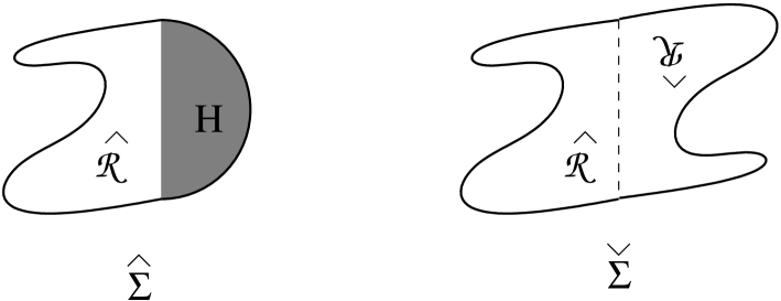
Figure 2: The geometry involved in computing the inner product of a surface state $|\Sigma\rangle$ with itself.

In this subsection we will address the computation of correlation functions of the form $\langle\Sigma|\prod_{i=1}^{n}{\cal O}_{i}(\xi_{i})|\Sigma\rangle$ with $\xi_{i}$’s lying on the unit circle. These are inner products of surface states with operator insertions. Such computations will play a role in our later analysis of split wave-functionals and half-string states. We will also discuss star products of surface states.

These computations are particularly simple in the representation of the surface $\Sigma$ in the $\widehat{w}$ coordinate system. Let $\widehat{\cal R}$ and $\widehat{\Sigma}$ denote the images of ${\cal R}$ and $\Sigma$ in the $\widehat{w}$ plane. Then we can rewrite eq.(2.2) as

$$\langle\Sigma|\phi\rangle=\langle h\circ\phi(0)\rangle_{\widehat{\Sigma}}\,,$$ (2.8)

where $h$ has been defined in eq.(2.5). To compute $\langle\Sigma|\prod_{i=1}^{n}{\cal O}_{i}(\xi_{i})|\Sigma\rangle$ we begin with two copies of $\widehat{\Sigma}$, remove the local coordinate patches from each so that we are left with two copies of $\widehat{\cal R}$, and then simply construct a new disk by gluing the left-half string of the first disk to the right half-string of the second string and vice versa, as shown in Fig.2. If we denote the new disk by $\check{\Sigma}$ then we have

$$\langle\Sigma|\prod_{i=1}^{n}{\cal O}_{i}(\xi_{i})|\Sigma\rangle=\langle\prod_{i=1}^{n}h\circ{\cal O}(\xi_{i})\rangle_{\check{\Sigma}}\,.$$ (2.9)

The $h\circ{\cal O}_{i}(\xi_{i})$ factors are inserted at the images of the points $\xi_{i}=e^{i\sigma_{i}}$ in the $\widehat{w}$ plane, i.e. on the imaginary axis.

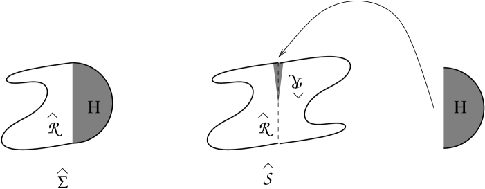
Figure 3: The geometry involved in computing the star product of a surface state with itself. The local coordinate patch, shown as the shaded half-disk to the right, is to be glued to the shaded region of the diagram representing $\widehat{\cal S}$.

We shall also need to compute the star product of a surface state with itself. This is again simple in the $\widehat{w}$ coordinate system. We begin with two copies of the disk $\widehat{\Sigma}$, remove the local coordinate patch from the second $\widehat{\Sigma}$, and then glue the right half-string of the first $\widehat{\Sigma}$ with the left half-string of the second $\widehat{\Sigma}$. The result is a new disk $\widehat{\cal S}$, as shown in Fig.3. As indicated in the figure, the local coordinate patch is glued in and thought as part of $\widehat{\cal S}$. The surface state $|{\cal S}\rangle$ associated with the new surface $\widehat{\cal S}$ gives $|\Sigma*\Sigma\rangle$. Thus we have:

$$\langle\Sigma*\Sigma|\phi\rangle=\langle h\circ\phi(0)\rangle_{\widehat{\cal S}}\,.$$ (2.10)

2.3 Operator representation of surface states

We shall now review the explicit representation of surface states in terms of Virasoro operators acting on the SL(2,R) invariant vacuum, rather than the implicit representation through correlators given eq.(2.3). Using the SL(2,R) invariance of the upper half plane, we can make the map $f$ appearing in eq.(2.3) satisfy $f(0)=f^{\prime\prime}(0)=0$, $f^{\prime}(0)=1$. We can write the corresponding surface state $\langle\Sigma|$ as

$$\langle\Sigma|=\langle 0|U_{f}\equiv\langle 0|\exp\left(\sum_{n=2}^{\infty}v_{n}^{(f)}L_{n}\right)\,,$$ (2.11)

where the coefficients $v_{n}^{(f)}$ are determined by the condition that the vector field

$$v(\xi)=\sum_{n=2}^{\infty}v_{n}^{(f)}\xi^{n+1}\,,$$ (2.12)

exponentiates to $f$,

$$\exp\left(v(\xi)\partial_{\xi}\right)\xi=f(\xi)\,.$$ (2.13)

We now consider the one-parameter family of maps

$$f_{\beta}(\xi)=\exp\Bigl{(}\beta\,v(\xi){\partial\over\partial\xi}\Bigr{)}\,\xi\,.$$ (2.14)

This definition immediately gives

$$\frac{d}{d\beta}f_{\beta}(\xi)=v(f_{\beta}(\xi))\,.$$ (2.15)

Solution to this equation, subject to the boundary condition $f_{\beta=0}(\xi)=\xi$, gives:

$$f_{\beta}(\xi)=g^{-1}(\beta+g(\xi))\,,$$ (2.16)

where

$$g^{\prime}(\xi)={1\over v(\xi)}\,.$$ (2.17)

Thus

$$f(\xi)=g^{-1}(1+g(\xi))\,.$$ (2.18)

Equations (2.17) and (2.18) readily give $f(\xi)$ if $v(\xi)$ is known. Alternatively, they also determine $v(\xi)$ in terms of $f(\xi)$, although not explicitly, since eqn. (2.18) is in general hard to solve for $g$. When a solution for $v(\xi)$ is available, eqn.(2.11) gives the operator expression for $|\Sigma\rangle$.

2.4 Oscillator representation of surface states

If the BCFT under consideration is that of free scalar fields with Neumann boundary condition describing D-25-branes in flat space-time, we can also represent the state in terms of the oscillators associated with the scalar fields. For simplicity let us restrict our attention to the matter part of the state only. If $a_{m}$, $a_{m}^{\dagger}$ denote the annihilation and creation operators associated with the scalar fields, then we have:

$$|\Sigma\rangle=\exp\left(-\frac{1}{2}\sum_{m,n=1}^{\infty}a^{\dagger}_{m}V^{f}_{mn}a^{\dagger}_{n}\right)|0\rangle\,.$$ (2.19)

where we have suppressed spacetime indices and [36]

$$V^{f}_{mn}={(-1)^{m+n+1}\over\sqrt{mn}}\oint_{0}{dw\over 2\pi i}\oint_{0}{dz\over 2\pi i}\,{1\over z^{m}w^{n}}{f^{\prime}(z)f^{\prime}(w)\over(f(z)-f(w))^{2}}\,.$$ (2.20)

Both $w$ and $z$ integration contours are circles around the origin, with the $w$ contour lying outside the $z$ contour, and both contours lying inside the unit circle. In eq.(2.19) we have also omitted an overall normalization factor.

We now show that when the vector field $v(\xi)$ generating the conformal map $f(\xi)$ is known (see the discussion in the previous subsection) the above integral expression for the matrix $V^{f}$ of Neumann coefficients can be given an alternate form which is sometimes easier to evaluate. For this purpose, we now consider the matrix $V(\beta)$ associated to the family of maps (2.14), and rewrite (2.20) as

$$V_{mn}(\beta)\equiv V_{mn}^{f_{\beta}}={(-1)^{m+n+1}\over\sqrt{mn}}\oint_{0}{dw\over 2\pi i}\oint_{0}{dz\over 2\pi i}\,{1\over z^{m}w^{n}}\frac{\partial}{\partial z}\frac{\partial}{\partial w}\log(f_{\beta}(z)-f_{\beta}(w))\,.$$ (2.21)

Taking a derivative with respect to the parameter $\beta$,

$$\displaystyle\frac{d}{d\beta}V_{mn}(\beta) = \frac{(-1)^{m+n+1}}{\sqrt{mn}}\oint_{0}{dw\over 2\pi i}\oint_{0}{dz\over 2\pi i}\,{1\over z^{m}w^{n}}\frac{\partial}{\partial z}\frac{\partial}{\partial w}\frac{\partial}{\partial\beta}\log(f_{\beta}(z)-f_{\beta}(w))\,$$

$$= \frac{(-1)^{m+n+1}}{\sqrt{mn}}\oint_{0}{dw\over 2\pi i}\oint_{0}{dz\over 2\pi i}\,{1\over z^{m}w^{n}}\frac{\partial}{\partial z}\frac{\partial}{\partial w}\left(\frac{v(f_{\beta}(z))-v(f_{\beta}(w))}{f_{\beta}(z)-f_{\beta}(w)}\right)\,,$$

where we have exchanged the order of derivatives and used (2.15). Integration by parts in $z$ and $w$ then gives

$$\frac{d}{d\beta}V_{mn}(\beta)={(-1)^{m+n+1}\sqrt{mn}}\oint_{0}{dw\over 2\pi i}\oint_{0}{dz\over 2\pi i}\,{1\over z^{m+1}w^{n+1}}\frac{v(f_{\beta}(z))-v(f_{\beta}(w))}{f_{\beta}(z)-f_{\beta}(w)}\,.$$ (2.23)

This is a general formula that we have found useful in concrete computations. If the above matrix is calculable, the desired Neumann coefficients $V_{mn}(\beta=1)$ are then readily obtained by integration over $\beta$.

2.5 Wave-functionals for surface states

In this subsection we wish to establish a dictionary between the geometric interpretation of surface states as one-punctured disks and their representation as wave-functionals of open string configurations. For this we consider open strings on a D-25-brane in flat space-time so that we have Neumann boundary condition on all the fields, and write, for a surface state associated to the map $z=f(\xi)$

$$\langle\Sigma|X(\sigma)\rangle={\cal N}_{f}\exp\left(-\frac{1}{2}\int_{0}^{\pi}\int_{0}^{\pi}d\sigma d\sigma^{\prime}X(\sigma)A_{f}(\sigma,\sigma^{\prime})X(\sigma^{\prime})\right)\,.$$ (2.24)

Here we have suppressed the Lorentz indices and used the fact that the wave-functional is in fact gaussian. This follows since the vacuum $|0\rangle$ is represented by a gaussian wave-functional, and the action of $U_{f}$ preserves this property. The normalization constant ${\cal N}_{f}$ is chosen so that $\langle\Sigma|\Sigma\rangle=1$. The wave-functional can also be represented in terms of modes:

$$\langle\Sigma|X\rangle={\cal N}_{f}\exp(-\frac{1}{2}\sum_{n,m=1}^{\infty}X_{n}A^{(f)}_{nm}X_{m})\,,$$ (2.25)

where we have adopted the convention of ref.[37] to define the modes $X_{n}$:

$$X(\sigma)=X_{0}+\sqrt{2}\sum_{n=1}^{\infty}X_{n}\cos(n\sigma)\,.$$ (2.26)

For simplicity we are considering the case where the coordinate $X$ has Neumann boundary condition. Using eqs.(2.24), (2.25), (2.26) we see that $A_{f}(\sigma,\sigma^{\prime})$ is related to $A^{(f)}_{nm}$ through the relation:

$$A_{f}(\sigma,\sigma^{\prime})={2\over\pi^{2}}\sum_{m,n\geq 1}A^{(f)}_{nm}\cos(n\sigma)\cos(m\sigma^{\prime})\,.$$ (2.27)

Note that $X_{0}$ does not appear in the expression for the wave-functional in (2.25), since all surface states are translationally invariant. We shall from now on restrict to twist-even surface states, which is equivalent to the condition that $f$ is an odd function.

The relation between the oscillator representation (2.19) and the wave-functional representation (2.25) is given by the following relation between the matrices $V^{f}$ and $A^{(f)}$[6, 11]:

$$A^{(f)}=2E^{-1}\,{1-V^{f}\over 1+V^{f}}\,E^{-1}\,,\qquad E_{nm}=\delta_{mn}\sqrt{2\over n}\,.$$ (2.28)

We want to determine $A_{f}(\sigma,\sigma^{\prime})$ from $f$. To this end, we evaluate the normalized correlator

$$B_{f}(\sigma_{1},\sigma_{2})\equiv\langle\Sigma|\partial_{\sigma_{1}}\hat{X}(\sigma_{1})\partial_{\sigma_{2}}\hat{X}(\sigma_{2})|\Sigma\rangle$$ (2.29)

in two different ways. First, we use the wave-functional representation and obtain

$$\displaystyle B_{f}(\sigma_{1},\sigma_{2}) = {\cal N}_{f}^{2}\int{\cal D}X\exp\left(-\int_{0}^{\pi}d\sigma d\sigma^{\prime}X(\sigma)A_{f}(\sigma,\sigma^{\prime})X(\sigma^{\prime})\right)\partial_{\sigma_{1}}X(\sigma_{1})\partial_{\sigma_{2}}X(\sigma_{2})$$ (2.30)

$$= \frac{1}{2}\partial_{\sigma_{1}}\partial_{\sigma_{2}}(A_{f}^{-1}(\sigma_{1},\sigma_{2}))\,.$$

Here the inverse kernel $A_{f}^{-1}(\sigma_{1},\sigma_{2})$ is defined by

$$\int_{0}^{\pi}d\sigma A_{f}(\sigma_{1},\sigma)A_{f}^{-1}(\sigma,\sigma_{2})=\delta(\sigma_{1}-\sigma_{2})-{1\over\pi}\,.$$ (2.31)

The constant $1/\pi$ in the above equation represents the contribution from the zero mode part. Since $A_{f}$ does not depend on the zero modes, it has an inverse only in the subspace spanned by the functions $\cos(n\sigma)$ for $n\neq 0$. Thus $(A_{f}^{-1})_{mn}$ is nonzero only for $m,n\geq 1$.

In the second computation, we interpret (2.29) as a CFT correlator on an appropriate Riemann surface following the procedure of section 2.2. This is nicely done using the $\widehat{z}$ presentation (see section 2.1) where the surface will occupy a region ${\cal C}_{f}$ in the $\widehat{z}$ plane, and the local coordinate patch is the strip $\Im(\widehat{z})\geq 0$, $-\pi/4\leq\Re(\widehat{z})\leq\pi/4$. As usual the vertical line corresponding to $\Re(\widehat{z})=\pi/4$ is the image of the left-half of the string, and the vertical line corresponding to $\Re(\widehat{z})=-\pi/4$ is the image of the right-half of the string. In order to compute a correlation function of the form $\langle\Sigma|\cdots|\Sigma\rangle$, we simple start with two copies of ${\cal C}_{f}$, strip off the local coordinate patch from each of them, and compute the correlation function on the surface obtained by gluing the left half-string on the first ${\cal C}_{f}$ with the right half-string on the second ${\cal C}_{f}$ and vice versa. Thus the right hand side of (2.29) can be computed by this method. If we denote the new surface by $\check{C}_{f}$, then $B_{f}$ is given by

$$B_{f}(\sigma_{1},\sigma_{2})=\partial_{\sigma_{1}}\partial_{\sigma_{2}}\langle X(\widehat{z}_{1})X(\widehat{z}_{2})\rangle_{\check{C}_{f}}\,,$$ (2.32)

where $\widehat{z}_{i}$ are the images of the points $\xi=e^{i\sigma_{i}}$. Comparing (2.30) with (2.32) we can determine $A_{f}^{-1}(\sigma_{1},\sigma_{2})$ and hence the wave-functional of the surface state.

Let us illustrate this for the vacuum state $|0\rangle$. In this case the CFT computation is immediate, since we can directly compute the correlator (2.29) using the OPE’s of X’s on the UHP,

$$\displaystyle B_{|0\rangle}(\sigma_{1},\sigma_{2}) = \partial_{\sigma_{1}}\partial_{\sigma_{2}}\Big{(}-\frac{1}{2}\log(|e^{i\sigma_{1}}-e^{i\sigma_{2}}|^{2}|e^{i\sigma_{1}}-e^{-i\sigma_{2}}|^{2})\Big{)}$$ (2.33)

$$= -\partial_{\sigma_{1}}\partial_{\sigma_{2}}\log(2\cos(\sigma_{1})-2\cos(\sigma_{2}))$$

$$= \partial_{\sigma_{1}}\partial_{\sigma_{2}}\sum_{n=1}^{\infty}\frac{2}{n}\cos(n\sigma_{1})\cos(n\sigma_{2})\,.$$

Using (2.30) and inverting the kernel, we get

$$A_{|0\rangle}(\sigma_{1},\sigma_{2})={2\over\pi^{2}}\sum_{n=1}^{\infty}n\cos(n\sigma_{1})\cos(n\sigma_{2})\,.$$ (2.34)

This gives

$$A^{|0\rangle}_{nm}=n\delta_{nm}\,.$$ (2.35)

This is the expected result, as can be seen by using eq.(2.28) with $V^{f}=0$.

3 Conformal Field Theories on Degenerate Disks

In this section we shall consider some properties of degenerate disks involving singular conformal maps, and of conformal field theories on such degenerate disks.

3.1 A conformal mapping claim

Consider a set of surfaces parametrized by $t\in[0,1]$. For each $t$ different from one, the surface $R(t)$ is a finite region of the complex plane with the topology of a disk (see figure 4). As $t$ goes to one the region varies smoothly throughout but develops a thin neck and at $t=1$ it pinches, breaking into two pieces $R_{1}$ and $R_{2}$, both of which are finite disks. Let $P$ denote the pinching point, common to $R_{1}$ and $R_{2}$, and assume there are no other pinching points. Because disks can always be mapped to disks, any $R(t)$ with $t<1$ can be mapped to $R_{1}$. The map in fact is not unique due to SL(2,R) invariance of the disk. We now claim that:

Claim: There exists a family of conformal maps $m(t):R(t)\to R_{1}$, for $t\in[0,1]$, continuous in $t$, where $m(1)$ is the identity map over $R_{1}$ and maps all of $R_{2}$ to $P$.

The intuition here is that as far as one of the sides of the pinching surface is concerned, call it side one, all that is going on on the other side, side two, can be viewed as happening near the pinching point. The complete side two, lying on the other side of the neck, can be mapped to a vanishingly small region while the conformal map is accurately close to the identity on side one. An explicit example of this will be given next.

Figure 4: The surface $R(t)$ is pinching for $t=1$. The pinching point $P$ separates the regions $R_{1}$ and $R_{2}$ of the surface $R(1)$.

3.2 A prototype example

To illustrate the claim in the above subsection we consider the following situation. Let a surface $\Sigma$ with the topology of a disk be the region in the $\hat{u}$-plane defined by $\Im(\hat{u})\geq-\pi$ with two cuts, both along the real axis, the first for real $\hat{u}\in(-\infty,-\Delta]$ and the second for real $\hat{u}\in[\Delta,+\infty)$ where $\Delta$ is a small positive real number. As illustrated as a shaded region in figure 5(a), this region is the upper half plane, joined through the small interval $\hat{u}\in[-\Delta,\Delta]$ to an infinite horizontal strip of width $\pi$. We have also marked some special points $P_{1},\cdots P_{n}$ at some real coordinates $\hat{u}(P_{i})$ with $|\hat{u}(P_{i})|\gg\Delta$, for all $i$.

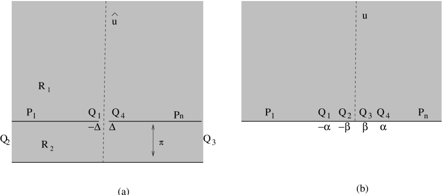
Figure 5: Illustration of a conformal map from the upper-half plane plus a strip of width $\pi$ connected by a narrow neck (part (a)) to the upper-half plane (part (b)).

This surface, in the limit $\Delta\to 0$, is pinching, and in the terminology of the claim, the region $R_{1}$ is the upper half $\hat{u}$-plane, and the region $R_{2}$ is the horizontal infinite strip of width $\pi$ in the lower half plane. We will now show that the surface can be mapped completely to the upper-half $u$ plane (figure 5(b)) such that the conditions in the claim are satisfied. Indeed, in the limit $\Delta\to 0$, the map will become the identity over the upper half plane ($R_{1}$) and will map all of the lower strip ($R_{2}$) into a point. We will also see that this is the limit of a family of maps that near degeneration leave $R_{1}$ mostly unchanged (in a quantifiable way).

The conformal map differential equation is readily written, as it is of Schwarz-Christoffel type. Noting that the turning points $Q_{1}$ and $Q_{4}$ are points of turning angle $(-\pi)$, while $Q_{2}$ and $Q_{3}$ are turning points of turning angle $(+\pi)$ we write:

$$d\hat{u}={u^{2}-\alpha^{2}\over u^{2}-\beta^{2}}\,\,du\,.$$ (3.1)

The turning points $Q_{1},Q_{2},Q_{3},Q_{4}$ are mapped to the points $\{-\alpha,-\beta,\beta,\alpha\}$ on the $u$-plane real axis, as shown in 5(b). We have two parameters $\{\alpha,\beta\}$ and two conditions, one defining the width of the strip, and the other specifying the separation $2\Delta$ between $Q_{1}$ and $Q_{4}$ in the $\hat{u}$ plane. The normalization above was fixed so that for large $u\gg\{\alpha,\beta\}$, we have $d\hat{u}\sim du$, – a necessary condition for the map to become the identity when $u$ and $\hat{u}$ are large. The condition that the strip corresponding to $R_{2}$ has width $\pi$ demands that the residues of the above right hand side at $u=\pm\beta$ be equal to $(\mp 1)$. This gives

$${\alpha^{2}-\beta^{2}\over 2\beta}=1\,.$$ (3.2)

With this condition, the differential relation in (3.1) becomes:

$$d\hat{u}=\Bigl{(}1-{1\over u-\beta}+{1\over u+\beta}\Bigr{)}\,\,du\,.$$ (3.3)

By symmetry, we require that $u=0$ correspond to $\hat{u}=-i\pi$ and thus we have that

$$\Delta=P\int_{0}^{\alpha}\Bigl{(}1-{1\over u-\beta}+{1\over u+\beta}\Bigr{)}\,\,\,du\,,$$ (3.4)

where $P$ denotes principal value, which must be taken at $u=\beta$. Evaluation gives

$$\Delta=\alpha+\ln\Bigl{(}{\alpha+\beta\over\alpha-\beta}\Bigr{)}\,.$$ (3.5)

It is clear from this equation that to have $\Delta$ small we need $\alpha$ small and $\beta\ll\alpha$. This, and the constraint in (3.2) can be satisfied with

$$\alpha=\sqrt{2\beta+\beta^{2}},\qquad\alpha,\beta\ll 1\quad\to\quad\beta\simeq{1\over 2}\alpha^{2}\,.$$ (3.6)

Note that given these relations, (3.5) gives us

$$\Delta=2\alpha+{\cal O}(\alpha^{2})\,,\quad\to\quad\Delta\simeq 2\alpha\,.$$ (3.7)

This shows that the whole boundary of the strip $R_{2}$, which is mapped to $u\in[-\alpha,\alpha]$, is indeed mapped to a vanishingly small segment as $\Delta\to 0$.

Finally, we confirm that the map goes to the identity map for $\{u,\hat{u}\}\gg\Delta$ when $\Delta\to 0$. For this purpose integrating from $\alpha$ to $u>\alpha$ we have

$$\hat{u}=\Delta+\int_{\alpha}^{u}\Bigl{(}1-{1\over u-\beta}+{1\over u+\beta}\Bigr{)}\,\,\,du\,,$$ (3.8)

which using (3.5) gives

$$\hat{u}=u+\ln\Bigl{(}{u+\beta\over u-\beta}\Bigr{)}\,,\quad u>\alpha\,.$$ (3.9)

Since $u>\alpha\gg\beta$ we have

$$\hat{u}\simeq u+{2\beta\over u}\simeq u+{\Delta^{2}\over 4u}\,\quad\to\quad u\simeq\hat{u}-{\Delta^{2}\over 4\hat{u}}\,.$$ (3.10)

This confirms that away from the pinching area the map goes to the identity map as $\Delta\to 0$.

3.3 Conformal field theory and factorization

Let us now consider a unitary s boundary conformal field theory on a surface $R(t)$ of the type described in section 3.1 and consider a correlation function of the form:

$$\langle\prod_{i=1}^{n}{\cal O}_{i}(z_{i})\rangle_{R(t)}\,.$$ (3.11)

${\cal O}_{i}$ could be bulk or boundary operators of the theory. We shall assume that all operators in the theory have dimension $>0$ except the identity operator which has dimension zero. Let us now consider the case where in the $t\to 1$ limit the points $z_{1},\ldots z_{m}$ lie inside the disk $R_{1}$ and the points $z_{m+1},\ldots z_{n}$ lie inside the disk $R_{2}$. In this limit, using the results of the previous subsection we can map the disk $R$ to the disk $R_{1}$ in such a way that the map is the identity inside $R_{1}$ and maps the whole of $R_{2}$ to a point $P$. Thus the insertion points $z_{m+1},\ldots z_{n}$ approach the point $P$. The correlation function on such a disk can be evaluated by picking up the leading terms in the operator product expansion of the appropriate conformal transforms of the operators ${\cal O}_{m+1},\ldots{\cal O}_{n}$. Since the lowest dimension operator in the theory is the identity operator, we get:

$$\langle\prod_{i=1}^{n}{\cal O}_{i}(z_{i})\rangle_{R(t=1)}=\langle\prod_{i=1}^{m}{\cal O}_{i}(z_{i})\rangle_{R_{1}}g(z_{m+1},\ldots z_{n})\,,$$ (3.12)

where $g(z_{m+1},\ldots z_{n})$ is the function that appears in evaluating the coefficient of the identity operator in the operator product expansion of the appropriate conformal transforms of ${\cal O}_{m+1},\ldots{\cal O}_{n}$.

On the other hand, we could also carry out the analysis using a different conformal transformation that maps the disk $R(1)$ to $R_{2}$ and maps the disk $R_{1}$ to the point $P$. In this case we have

$$\langle\prod_{i=1}^{n}{\cal O}_{i}(z_{i})\rangle_{R(t=1)}=\langle\prod_{i=m+1}^{n}{\cal O}_{i}(z_{i})\rangle_{R_{2}}f(z_{1},\ldots z_{m})\,.$$ (3.13)

Combining eqs.(3.12) and (3.13), and normalizing the correlator so that the $\langle{\bf 1}\rangle_{\Sigma}=1$ on any disk $\Sigma$, we get

$$\langle\prod_{i=1}^{n}{\cal O}_{i}(z_{i})\rangle_{R(t=1)}=\langle\prod_{i=1}^{m}{\cal O}_{i}(z_{i})\rangle_{R_{1}}\,\,\langle\prod_{i=m+1}^{n}{\cal O}_{i}(z_{i})\rangle_{R_{2}}\,.$$ (3.14)

Thus the correlation function on the splitting surface factors into the product of correlation functions of the separate surfaces.

4 Split wave-functionals and Half-string States

In this section we will show that the split wave-functional property of surface states holds when the boundary of the surface reaches the open string midpoint. This is a very general statement, and our purpose here will be to explain it just based on the conformal mapping properties of pinching surfaces, and the factorization properties of CFT correlators, both of which were discussed in the previous sections. In the process we shall find an explicit surface state construction of half-string states that emerge from the split wave-functional. Throughout this section we shall focus on the matter part of the surface state only.

4.1 Factorization of the string wave-functional

We shall examine the condition under which a string state $|\Psi\rangle$ gives rise to a wave-functional $\Psi[X(\sigma)]$ that factorizes into a functional of the left half of the string and a functional of the right half of the string. As is clear from the discussion of section 2.5, all information about the wave-functional associated to a state $|\Psi\rangle$ is contained in correlation functions of the form

$$\langle\Psi|\prod_{i=1}^{n}{\cal O}_{i}(\xi_{i})|\Psi\rangle=\int[{\cal D}X(\sigma)]\prod_{i=1}^{n}\widetilde{\cal O}_{i}(X(\sigma_{i}))\Psi[X(\pi-\sigma)]\Psi[X(\sigma)]\,,$$ (4.1)

where $\xi_{i}=e^{i\sigma_{i}}$, ${\cal O}_{i}$ denote an arbitrary set of local vertex operators, and $\widetilde{\cal O}_{i}$ are these vertex operators viewed as classical functionals of $X(\sigma)$. Let us consider the case where $\sigma_{i}$ for $1\leq i\leq m$ lie in the range $[0,\pi/2)$, and $\sigma_{i}$ for $(m+1)\leq i\leq n$ lie in the range $(\pi/2,\pi]$. If the wave-functional is factorized into a functional $\Phi_{L}$ of the coordinates of the left-half of the string ($X(\sigma)$ for $0\leq\sigma<\pi/2$) and a functional $\Phi_{R}$ of the coordinates of the right-half of the string ($X(\sigma)$ for $\pi/2<\sigma\leq\pi$):

$$\Psi[X(\sigma)]=\Phi_{L}[X(2\sigma)]\Phi_{R}[X(2(\pi-\sigma))]\,.$$ (4.2)

Note that the parametrization of the right half-string has reversed direction; as $\sigma$ increases we move towards the full string midpoint, just as for the left half-string. It now follows that the correlation function (4.1) has the factorized form:

$$\langle\Psi|\prod_{i=1}^{n}{\cal O}_{i}(\xi_{i})|\Psi\rangle=f(\sigma_{1},\ldots\sigma_{m})\,g(\sigma_{m+1},\ldots\sigma_{n})\,.$$ (4.3)

Alternatively, if eq.(4.3) is satisfied by all such correlation functions, we can conclude that $\Psi$ has a factorized wave-functional. This will be our test of factorization.

Furthermore, if $|\Phi_{L}\rangle$ and $|\Phi_{R}\rangle$ denote the states associated with the left and the right half of the string respectively, then we have:

$$f(\sigma_{1},\ldots\sigma_{m})=\langle\Phi_{R}^{c}|\prod_{i=1}^{m}s\circ{\cal O}_{i}(\xi_{i})\,|\Phi_{L}\rangle\,,$$ (4.4)

where $s$ denotes the conformal transformation $s:\xi\to\xi^{2}$ and the superscript $c$ denotes twist transformation: $\sigma\to(\pi-\sigma)$, needed for the right half-string. Here the conformal transformation $s$ rescales the coordinate $\sigma$ so that the coordinate labeling the left half-string runs from 0 to $\pi$. Similarly we have

$$g(\sigma_{m+1},\ldots\sigma_{n})=\langle\Phi_{R}^{c}|\prod_{i=m+1}^{n}\tilde{s}\circ{\cal O}_{i}(\xi_{i})\,|\Phi_{L}\rangle\,,$$ (4.5)

where $\tilde{s}$ denotes the conformal transformation $\xi\to\xi^{-2}$.

Figure 6: The geometry of the disks $\widehat{\Sigma}$ and $\check{\Sigma}$ when the boundary of $\widehat{\Sigma}$ touches the string midpoint.

We shall now show that (4.3) is satisfied for $|\Psi\rangle=|\Sigma\rangle$ if any part of the boundary of ${\cal R}$, – the part of the disk $\Sigma$ outside the local coordinate patch – touches the point $\xi=i$, or equivalently, if in the $\widehat{w}$ plane any part of the boundary of $\widehat{\cal R}$ touches the point $\widehat{w}=0$. Such a situation has been shown in Fig.6(a). According to the general result discussed in section 2.2, the left hand side of (4.3) for $|\Psi\rangle=|\Sigma\rangle$ is expressed as a correlation function on a surface $\widehat{\cal S}$, obtained by gluing together two copies of $\widehat{\cal R}$ along the procedure illustrated in Fig.2. In the present context, the gluing of two such disks produces a disk $\check{\Sigma}$ which is pinched at the origin of the $\widehat{w}$ plane, as shown in Fig.6(b). In the diagram the images of the points $\sigma_{1},\ldots\sigma_{m}$, lying on the left half-string, are on the positive imaginary axis, whereas those of the points $\sigma_{m+1},\ldots\sigma_{n}$, lying on the right half-string, are on the negative imaginary axis. $\check{\Sigma}$ can be viewed as the union of two disks $\widehat{\cal N}$ and $r\circ\widehat{\cal N}$, joined at the origin, where $r$ denotes the conformal map $\widehat{w}\to-\widehat{w}$. Since the total surface is pinched, the conformal field theory results of section 3.3 hold, and working with normalized correlation functions so that the partition function on a disk equals one, the correlation function (2.9) factorizes as

$$\langle\prod_{i=1}^{n}h\circ{\cal O}(\xi_{i})\rangle_{\check{\Sigma}}\,=\langle\prod_{i=1}^{m}h\circ{\cal O}(\xi_{i})\rangle_{\widehat{\cal N}}\,\,\langle\prod_{i=m+1}^{n}h\circ{\cal O}(\xi_{i})\rangle_{r\circ\widehat{\cal N}}\,.$$ (4.6)

This establishes eq.(4.3). Furthermore this gives:

$$f(\sigma_{1},\ldots\sigma_{m})=\langle\prod_{i=1}^{m}h\circ{\cal O}(\xi_{i})\rangle_{\widehat{\cal N}}\,.$$ (4.7)

Comparing with eq.(4.4) we have:

$$\langle\Phi_{R}^{c}|\prod_{i=1}^{m}s\circ{\cal O}_{i}(\xi_{i})\,|\Phi_{L}\rangle=\langle\prod_{i=1}^{m}h\circ{\cal O}_{i}(\xi_{i})\rangle_{\widehat{\cal N}}\,=\langle\prod_{i=1}^{m}s\circ{\cal O}_{i}(\xi_{i})\rangle_{s\circ h^{-1}\circ\widehat{\cal N}}\,.$$ (4.8)

where in the last step we used the conformal invariance of the correlator to act on the region $\widehat{\cal N}$ first by the $h^{-1}$ conformal map, and then by $s$. If the region $s\circ h^{-1}\circ\widehat{\cal N}$ is simple enough the explicit identification of the half string state is possible.

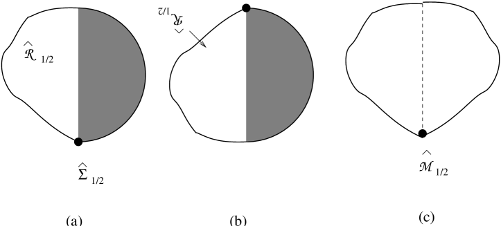
Figure 7: Fig. (a) shows the the disk associated with a a surface state, describing the state of the half-string, in the $\widehat{w}$ plane. Fig.(b) shows the twist conjugate of the surface state of Fig.(a). Fig.(c) shows the result of computing inner product between these two stares. $\widehat{\cal M}_{1/2}$ in this figure is the union of $\widehat{R}_{1/2}$ with its image under a reflection about the imaginary axis. The dots signal the half-string endpoint corresponding to the full-string midpoint. The other half- string endpoint coincides with one of the end-points of the original string.

4.2 Half-string surface states

The above results lead to a representation of the state of the half-string as a surface state. For convenience, let us restrict ourselves to the case where the original projector was twist invariant, which in this context means that $\widehat{\Sigma}$ (and hence $\widehat{\cal R}$) are symmetric under reflection about the real axis. Thus for these states $|\Phi_{L}\rangle=|\Phi_{R}\rangle\equiv|\Phi\rangle$. In that case we can rewrite eq.(4.8) as

$$\langle\Phi^{c}|\prod_{i=1}^{m}s\circ{\cal O}_{i}(\xi_{i})\,|\Phi\rangle=\langle\prod_{i=1}^{m}s\circ{\cal O}_{i}(\xi_{i})\rangle_{s\circ h^{-1}\circ\widehat{\cal N}}\,.$$ (4.9)

Let us take as a trial solution for $\langle\Phi^{c}|$ a surface state, represented by a disk $\widehat{\Sigma}_{1/2}$ in the $\widehat{w}$ coordinate system, so that

$$\langle\Phi^{c}|\phi\rangle=\langle h\circ\phi(0)\rangle_{\widehat{\Sigma}_{1/2}}\,.$$ (4.10)

As usual we denote by $\widehat{\cal R}_{1/2}$ the part of $\widehat{\Sigma}_{1/2}$ with local coordinate patch removed. This has been shown in Fig.7(a). The surface state associated with $\langle\Phi|$ will have an associated $\widehat{\cal R}$ which is the reflection of $\widehat{\cal R}_{1/2}$ about the real axis. This has been shown in Fig.7(b). In this case, we can represent the left hand side of (4.9) as

$$\langle\Phi^{c}|\prod_{i=1}^{m}s\circ{\cal O}_{i}(\xi_{i})\,|\Phi\rangle=\langle\prod_{i=1}^{m}h\circ s\circ{\cal O}_{i}(\xi_{i})\rangle_{\widehat{\cal M}_{1/2}}\,,$$ (4.11)

where $\widehat{\cal M}_{1/2}$ represents the disk obtained by the union of $\widehat{\cal R}_{1/2}$ with its image under a reflection about the imaginary axis. This has been shown in Fig.7(c). The operators $h\circ s\circ{\cal O}_{i}(\xi_{i})$ are inserted on the dotted line in this figure. We can rewrite this equation as

$$\langle\Phi^{c}|\prod_{i=1}^{m}s\circ{\cal O}_{i}(\xi_{i})\,|\Phi\rangle=\langle\prod_{i=1}^{m}s\circ{\cal O}_{i}(\xi_{i})\rangle_{h^{-1}\circ\widehat{\cal M}_{1/2}}\,.$$ (4.12)

Comparing (4.9) and (4.12) we get

$$\widehat{\cal M}_{1/2}=h\circ s\circ h^{-1}\circ\widehat{\cal N}\,.$$ (4.13)

Let $\widehat{\cal R}_{top}$ denote the top wing of $\widehat{\cal R}$ associated with the original projector describing a state of the full string. This is what has been labeled as the region $A$ in Fig.6(a). Given that for twist invariant state the region $B$ in Fig.6(a) is related to the region $A$ by a reflection about the real axis, we see from Fig.6(b) that the region $\widehat{\cal N}$ is the union of $\widehat{\cal R}_{top}$ with its reflection about the imaginary axis. On the other hand we have already seen that $\widehat{\cal M}_{1/2}$ is the result of the union of $\widehat{\cal R}_{1/2}$ with its reflection $I$ about the imaginary axis. Finally, it can be easily seen that conjugation by $h\circ s\circ h^{-1}$ leaves invariant the reflection $I$. Thus (4.13) implies that:

$$\widehat{\cal R}_{1/2}=h\circ s\circ h^{-1}\,\circ\widehat{\cal R}_{top}\,.$$ (4.14)

Conversely

$$\widehat{\cal R}_{top}=h\circ s^{-1}\circ h^{-1}\,\circ\widehat{\cal R}_{1/2}\,.$$ (4.15)

These equations show how to pass back and forth from the split full-string surface state to the associated half-string surface state. We will use this strategy to identify the half-string state associated to the butterfly.

Before concluding this section we would like to explain an issue concerning boundary conditions. From Fig.6(a) we see that other than the part of the boundary representing the string, the boundary of the region $A$ (called $\widehat{\cal R}_{top}$ in the current discussion) has boundary condition identical to that of the original disk $\widehat{\Sigma}$, since this part of the boundary of $A$ comes from part of the boundary of $\widehat{\Sigma}$. Eq.(4.14) then implies that the disk $\widehat{\cal R}_{1/2}$ also has the same boundary condition. Thus the half-string state is given by the surface state associated with the disk $\widehat{\Sigma}_{1/2}$ in the $\widehat{w}$-coordinate system, with the same boundary condition as that in the original full string surface state.

This, however, does not imply that both the half-string end-points satisfy the same boundary conditions as the end-points of the original string, since, as we now explain, the surface states defined with certain boundary conditions may actually fail to satisfy the boundary condition. In a surface state “the open string” is a specific line with endpoints at the boundary – in the $\widehat{w}$ presentation it is the vertical boundary of the shaded region called H. Consider a boundary condition of Neumann type. This is the statement that the normal derivative of fields at the boundary vanishes. We may thus expect on a surface state to find that the expectation values of the operator $\partial_{\sigma}{X}(\sigma)$ vanish at $\sigma=0,\pi$. But this vanishing will only happen if the tangent to the open string at the boundary coincides with the normal derivative to the boundary. This need not be the case when the boundary has corners at the open string endpoints. Corners at the open string endpoints happen when the map $z=f(\xi)$ has singularities at the points $\xi=\pm 1$. While this is not the case for slivers nor butterflies, we will see examples of this phenomenon in section 9.1.

In the case of half-string states associated to projectors, the above subtleties are in fact quite generic. If the original projector is such that the tangent to the open string coincides with the normal to the boundary, the corresponding half-string endpoint will carry the boundary condition (this is the case illustrated in figure 7). On the other hand the nature of the boundary near the full string midpoint, which is controlled by the behavior of $f(\xi)$ near $\xi=i$, will tell whether or not the boundary condition is satisfied at the other half-string endpoint. Getting a little ahead of ourselves we can have a look at the butterfly state, in particular at figure 9(d). Note that the tangent to the half-string AQ at Q is indeed along the normal to the boundary DQ at Q. Thus we may expect the half-string state for the butterfly to satisfy Neumann boundary conditions at both endpoints. It does, because as it will be checked, the half string state is simply the vacuum state. On the other hand, for a generalized butterfly, such as that shown in figure 19 the two directions do not coincide and we do not expect the half-string state to satisfy a simple boundary condition. For the nothing state, shown in figure 17, the normal to the boundary at the midpoint is orthogonal to the open string tangent. Thus the interpretation here is that $\partial_{\tau}\widehat{X}$ vanishes at this point. This is a Dirichlet boundary condition.

The above considerations may be relevant for understanding the applicability of the two different half-string formalisms [38], $-$ one where the mid-point satisfies Dirichlet boundary condition [39] and the other where the midpoint satisfies Neumann boundary condition [40]. We now see that for half-string states arising from projectors, neither formalism is natural in all cases. Since the set of functions are (at least formally) complete, we can use either formalism, but the results will take simplest forms when the boundary conditions match those that arise geometrically at the string midpoint.

5 Star Algebra Projectors

In this section we will show that the projection property of surface states also holds when the boundary of the surface reaches the open string midpoint. We will explain why the projectors that arise are of rank one. Finally we will prove that the Neumann matrix of any projector has a common eigenvector, the $-1/3$ eigenvector of the star algebra Neumann matrices. An intuitive explanation for this fact is given.

5.1 Projection properties

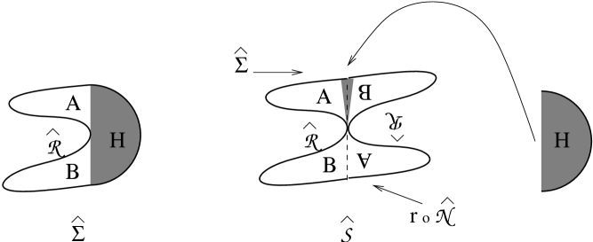
Figure 8: The geometry of $\widehat{\cal S}$ when the boundary of $\widehat{\Sigma}$ touches the string midpoint. The local coordinate patch, shown to the right by the shaded half disk, is to be glued to the shaded region of the diagram representing $\widehat{\cal S}$.

A surface state $|\Sigma\rangle$ defined as in (2.8) will be called a projector if it satisfies:

$$|\Sigma*\Sigma\rangle=|\Sigma\rangle\,.$$ (5.1)

We shall show that a surface states $|\Sigma\rangle$ is a projector if the corresponding surface $\Sigma$ has the property that the boundary of $\Sigma$ touches the string mid-point $\xi=i$, – the same condition under which its wave-functional factorizes. However, unlike in the previous section, in this subsection we shall work with the full surface state in the matter-ghost conformal field theory so that the total central charge vanishes, and the gluing relations required for the computation of $*$-product are valid without any additional multiplicative factors. For computing $|\Sigma*\Sigma\rangle$ we follow the procedure described in section 2.2. In this case the surface $\widehat{\cal S}$ that appears in eq.(2.10), constructed following Fig.3, is the pinched union of $\widehat{\Sigma}$ and an extra disk $r\circ\widehat{\cal N}$ as shown in Fig.8. We have, as in eq.(2.10),

$$\langle\Sigma*\Sigma|\phi\rangle=\langle h\circ\phi(0)\rangle_{\widehat{\cal S}}\,.$$ (5.2)

The operator $h\circ\phi(0)$ is being inserted on the $\widehat{\Sigma}$ component of $\widehat{\cal S}$, on the boundary of $H$, as usual. Hence there is no operator insertion on $r\circ\widehat{\cal N}$. Our factorization result of section 3.3 implies that the correlator factorizes and the contribution of $r\circ\widehat{\cal N}$ is simply a multiplicative factor of one. Thus eq.(5.2) can be rewritten as:

$$\langle\Sigma*\Sigma|\phi\rangle=\langle h\circ\phi(0)\rangle_{\widehat{\Sigma}}\,.$$ (5.3)

But the above right hand side is precisely $\langle\Sigma|\phi\rangle$ and therefore this establishes (5.1).

There is also a nice geometrical understanding that projectors that arise as surface states of the type discussed above are of rank one, – at least in a limited sense. For operators on separable Hilbert spaces, a projector $P$ is of rank one if and only if $PAP=\hbox{Tr}(AP)\,P$ for all $A$. Let now $\Sigma$ be a surface state projector $\Sigma*\Sigma=\Sigma$, and let $\Upsilon$ denote an arbitrary state of the star algebra (a Fock space state, or a surface state, for example). We then claim that the condition characterizing $\Sigma$ as a rank one projector holds:

$$\Sigma*\Upsilon*\Sigma=\langle\Sigma|\Upsilon\rangle\,\Sigma\,.$$ (5.4)

This equation is understandable in terms of pictures. Back to Fig.8, the above left hand side would be represented by a modified $\widehat{\cal S}$ where the $r\circ\widehat{\cal N}$ disk would be changed by cutting open the dashed line separating the sides $B$ and $A$, and gluing in the state $\Upsilon$. The new $r\circ\widehat{\cal N}$ disk, still pinched with respect to the remaining surface $\widehat{\Sigma}$ would be producing the $\langle\Sigma|\Upsilon\rangle$ inner product. The factorization implied by the pinching of the surfaces then yields (5.4).

There is, however, a subtlety involved in the derivation of (5.4) which we now discuss. In order to apply the factorization results of section 3.3 we need a unitary BCFT – otherwise the contribution from operators of negative dimension to the operator product expansion will invalidate (3.14). Thus (5.4) is not valid in general for the combined matter-ghost system, but could be valid for example for the matter part of the surface state. On the other hand since the matter part of the BCFT has a non-zero central charge, gluing of surface states typically involve (possibly infinite) multiplicative factors. Thus we expect (5.4) to be valid for the matter part of the state up to an overall multiplicative factor that depends only on the central charge of the matter BCFT and does not depend on the state $|\Upsilon\rangle$ or the particular BCFT under consideration. Alternatively, (5.4) is valid without any additional multiplicative factor in the combined matter-ghost BCFT if we restrict $|\Upsilon\rangle$ to be a state of ghost number 0, so that the leading contribution to the factorization relation comes from the identity operator as has been assumed in the derivation of (3.14).

5.2 A universal eigenvector of $V^{f}$ for all projectors

Give a projector of the type described above, we can use the procedure of section 2.3 to represent it as the exponentials of matter (and ghost) oscillators acting on the vacuum as in (2.19). We shall now show that the matrix $V^{f}_{mn}$ associated with any projector has the property that it has an eigenvector of eigenvalue one, the eigenvector being the same as the $\kappa=0$ eigenvector of $K_{1}$[21]. This generalizes the same property obeyed by the sliver Neumann matrix.

We start with (2.20) and integrate by parts with respect to $w$,

$$\displaystyle V^{f}_{mn}={(-1)^{m}\over\sqrt{m}}\oint{dw\over 2\pi i}\oint{dz\over 2\pi i}{1\over z^{m}}{f^{\prime}(z)\over f(z)-f(w)}\,\sqrt{n}\,\Bigl{(}-{1\over w}\Bigr{)}^{n+1}\,.$$ (5.5)

For definiteness we shall take the $w$ contour to be outside the $z$ contour. Acting on an eigenvector with components $v_{n}$ we find

$$\displaystyle\sum_{n=1}^{\infty}V^{f}_{mn}\,v_{n}={(-1)^{m}\over\sqrt{m}}\oint{dw\over 2\pi i}\oint{dz\over 2\pi i}{1\over z^{m}}{f^{\prime}(z)\over f(z)-f(w)}\,\,{1\over w^{2}}\sum_{n=1}^{\infty}\sqrt{n}\,v_{n}\Bigl{(}-{1\over w}\Bigr{)}^{n-1}\,.$$ (5.6)

We have argued that for all sufficently well-behaved maps $f(\xi)$ such that $f(\pm i)=\infty$, $\Psi_{f}$ is a projector. We now show that $f(\pm i)=\infty$ suffices to show that the $C$-odd $\kappa=0$ eigenvector $v^{-}$ of the Neumann matrices is in fact an eigenvector of eigenvalue one for the matrix $V^{f}$. The eigenvector in question is defined by the generating function

$$\sum_{n=1}^{\infty}{v_{n}^{-}\over\sqrt{n}}\,u^{n}=\tan^{-1}u\quad\to\quad\sum_{n=1}^{\infty}\sqrt{n}v_{n}^{-}\,u^{n-1}={1\over 1+u^{2}}\,\qquad|u|<1.$$ (5.7)

For regulation purposes we pick a number $a$ slightly bigger than one and write

$$\sum_{n=1}^{\infty}\sqrt{n}v_{n}^{-}\,u^{n-1}={1\over 1+(u/a)^{2}}\,,\qquad|u|<a\,,$$ (5.8)

with the understanding that the limit $a\to 1^{+}$ is to be taken. Therefore back in (5.6) we get

$$\displaystyle\sum_{n=1}^{\infty}V_{mn}\,v_{n}^{-}={(-1)^{m}\over\sqrt{m}}\oint{dw\over 2\pi i}\oint{dz\over 2\pi i}{1\over z^{m}}{f^{\prime}(z)\over f(z)-f(w)}\,\,{a^{2}\over 1+a^{2}w^{2}}\,,\quad|w|>\frac{1}{a}.$$ (5.9)

The $w$ integral must run over a contour of radius bigger than $1/a$ because of the use of (5.7) with $w=-1/u$. At the same time the radius of the contour must be less than 1 so that the contour does not enclose the singularities at $w=\pm i$. Therefore we pick up contributions from the poles at $w=\pm i/a$ and $w=z$. After this we can take the $a\to 1$ limit. Since $f(\pm i)=\infty$, only the $w=z$ pole contributes and we get

$$\displaystyle\sum_{n}V_{mn}v_{n}^{-}={(-1)^{m+1}\over\sqrt{m}}\oint{dz\over 2\pi i}{1\over z^{m}}{1\over 1+z^{2}}=v_{m}^{-}\,.$$ (5.10)

This establishes the claim.

An intuitive explanation for this property can be given using the half-string interpretation. The eigenvector in question implies that the projector wave-functional is invariant under constant and opposite translation of the half-strings [34]. If we denote by $P_{L}$ and $P_{R}$ respectively the momentum carried by the left and right half-strings we have that the eigenvector condition is interpreted as the condition that

$$(P_{L}-P_{R})|\Sigma\rangle=0\,,$$ (5.11)

where $|\Sigma\rangle$ is the projector surface state. Being a surface state defined with Neumann boundary condition (in the sense described in section 4.2), the total momentum $P_{L}+P_{R}$ carried by the state vanishes. Thus the condition above is simply the statement that $P_{L}$ and $P_{R}$ annihilate $|\Sigma\rangle$. But this must be so, since $|\Sigma\rangle=|\Sigma_{L}\rangle\otimes|\Sigma_{R}\rangle$, where $|\Sigma_{L}\rangle$ and $|\Sigma_{R}\rangle$ are themselves surface states defined with Neumann boundary condition.

6 The Butterfly State

In this section we shall introduce and investigate in detail the butterfly surface state. After giving the details of its definition and viewing it in various possible ways we shall verify that it is a projector of the star algebra. Throughout this section except in section 6.4 we shall work in the combined matter-ghost system with zero central charge so that we can apply the gluing theorem without any additional factors coming from conformal anomaly.

6.1 A picture of the butterfly

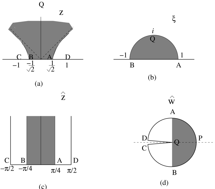
Figure 9: Representation of the disk associated with the butterfly state in various coordinate systems. The shaded region denotes the local coordinate patch.

The butterfly state, just as any surface state, is completely defined by a map from $\xi$ to the upper half $z$ plane ($z$-presentation, as reviewed in section 2.1). We thus write

$$z={\xi\over\sqrt{1+\xi^{2}}}\equiv f_{{\cal B}}(\xi)\,,$$ (6.1)

and define the butterfly state $|{\cal B}\rangle$ through the relation:

$$\langle{\cal B}|\phi\rangle=\langle f_{\cal B}\circ\phi(0)\rangle_{UHP}\,.$$ (6.2)

In the $z$-presentation the surface is the full upper half plane, and therefore in order to gain intuition about the type of state this is, we plot the image of the canonical $\xi$ half-disk in the $z$-plane (see Fig. 9 (a) and (b)). The open string $|\xi|=1,\Im(\xi)\geq 0$ is seen to map to the hyperbola $x^{2}-y^{2}={1\over 2}$ (in the upper half plane, with $z=x+iy$). We note that $z(\xi=i)=\infty$ and thus, as expected for a projector, the open string midpoint coincides with the boundary of the disk.

Further insight into the nature of the state is obtained by examination of the disk in the $\widehat{z}$-presentation. To this end we use (2.4) to recognize that (6.1) can be rewritten as

$$z=\sin(\tan^{-1}(\xi))=\sin\widehat{z}$$ (6.3)

This maps the image of the local coordinate in the $\widehat{z}$-presentation to the image of the local coordinate in the $z$-presentation. As explained before, the surface need not fill the upper-half $\widehat{z}$-plane. To figure out the extension of the surface in the $\widehat{z}$ presentation we simply invert the previous equation to write

$$\widehat{z}=\sin^{-1}z\,.$$ (6.4)

As shown in the figure (9 (c)), this transformation maps the full upper half $z$-plane into the region $|\Re(\widehat{z})|\leq\pi/2\,,\Im(\widehat{z})\geq 0$. Note that the vertical lines $\Re(\widehat{z})=\pm\pi/2$ are images of the boundary and not identification lines. Even though the surface occupies a portion of the $\widehat{z}$-plane the boundary reaches the point at infinity, and so does the midpoint (as expected). The above conformal map is perhaps most easily thought about in differential form, where it belongs to the class of Schwarz-Christoffel transformations. We have

$$d\widehat{z}={dz\over\sqrt{(1-z)(1+z)}}$$ (6.5)

The real line in the $z$-plane is mapped into a polygon in the $\widehat{z}$ presentation, where the turning points are $z=\pm 1$ and the turning angles are both $\pi/2$. This, of course is the result shown in the figure.

Finally, we give the $\widehat{w}$ presentation (fig. 9(d)). Using (2.6) the region $|\Re(\widehat{z})|\leq\pi/2\,,\Im(\widehat{z})\geq 0$ of the $\widehat{z}$ presentation turns into the full disk with a pair of cuts zooming into the $\widehat{w}$ origin from $\widehat{w}=-1$. Indeed the boundary of the surface is the arc $e^{i\theta}$ with $0<\theta<\pi$ together with the line going from $\widehat{w}=-1$ to $\widehat{w}=0$, plus the backwards line from $\widehat{w}=0$ to $\widehat{w}=-1$ plus the arc $e^{i\theta}$ with $-\pi<\theta<0$. It is perhaps in this presentation that it is clearest that the string midpoint $\widehat{w}=0$ touches the boundary of the disk.

6.2 The regulated butterfly

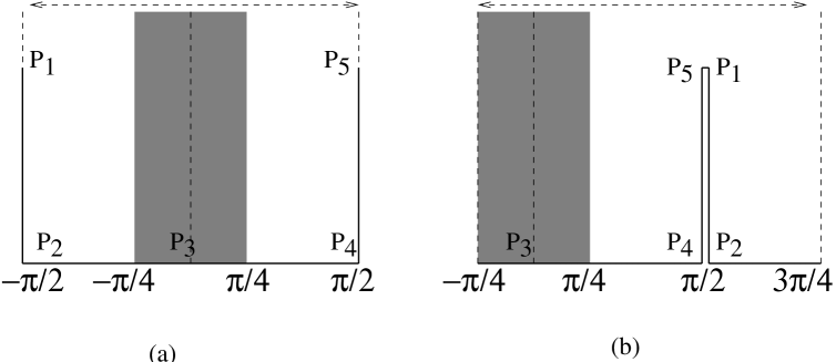
Figure 10: The geometry of the disk associated with the regularized butterfly in the complex $\widehat{z}$ plane. The shaded region denotes the local coordinate patch. The lines $\Re(\widehat{z})=-\pi/4$, $\Re(\widehat{z})=3\pi/4$ are identified in the second figure.

In order to regulate the butterfly it is simplest to do it in the $\widehat{w}$ coordinates. Here we simply stop the cut at some point $\widehat{w}_{0}$ with $-1<\widehat{w}_{0}<0$ a real negative number. In the $\widehat{z}$- presentation this turns into a picture shown in fig 10 (a). Note that the vertical lines $\Re(\widehat{z})=\pm\pi/2$ are not all boundary. Indeed the segments $\overline{P_{1}P_{2}}$ and $\overline{P_{4}P_{5}}$ are part of the boundary, but the remaining parts of the vertical lines, shown dashed in the figure, are identification lines. For more clarity and also later convenience we have shown in fig. 10(b) the same regulated butterfly where the region to the left of the right-half string has been moved, and the two extreme vertical lines are identified.

Figure 11: The singular points of the map $z\to\widehat{z}$ for the regulated butterfly in the $z$-plane.

In order to find the relation between $z$ and $\widehat{z}$ in the regulated butterfly we must construct the map, which is a variation on (6.5). In order to produce the identification shown by dashed lines, while preserving the property that the real line is mapped to a polygon a pair of complex conjugate poles are necessary. We write

$$d\widehat{z}={dz\over(1+\beta^{2}z^{2})\sqrt{1-z^{2}t^{2}}}$$ (6.6)

where we have fixed the normalization from the condition ${d\widehat{z}\over dz}=1$ at $z=0$. The images of the marked points $P_{1},\ldots P_{5}$ in Fig.10(a) in the $z$-plane is indicated in figure 11. The identification lines emerge from the pole at $z=i/\beta$. Since the identification lines differ by $\Delta\widehat{z}=\pi$ the residue at the pole $z=i/\beta$ in (6.6) must equal ${1\over 2i}$. This requires $\beta^{2}=1-t^{2}$ and thus we have

$$d\widehat{z}={dz\over(1+(1-t^{2})z^{2})\sqrt{1-z^{2}t^{2}}}\,.$$ (6.7)

This equation is readily integrated to give

$$\widehat{z}=\tan^{-1}\Bigl{(}{z\over\sqrt{1-z^{2}t^{2}}}\Bigr{)}\,,$$ (6.8)

and inverting the relation one finds

$$z={\tan\widehat{z}\over\sqrt{1+t^{2}\tan^{2}\widehat{z}}}={\xi\over\sqrt{1+t^{2}\xi^{2}}}\,.$$ (6.9)

This is a rather simple result. The regulator parameter $t$ can be related to the height $h$ of the points $P_{1}$ or $P_{5}$. Say, for $P_{5}$, $\widehat{z}(P_{5})={\pi\over 2}+ih$ must map to $z=\infty$. This requires $1+t^{2}\tan^{2}({\pi\over 2}+ih)=0$. A short calculation gives

$$h=\tanh^{-1}t\,,\quad\quad\hbox{thus}\quad h\to\infty\quad\hbox{when}\quad t\to 1^{-}\,.$$ (6.10)

The regulator parameter $t$ must therefore satisfy $t<1$. Clearly when $t=1$ in (6.9) we recover the butterfly as defined in (6.1).

6.3 Star multiplying two regulated butterflies

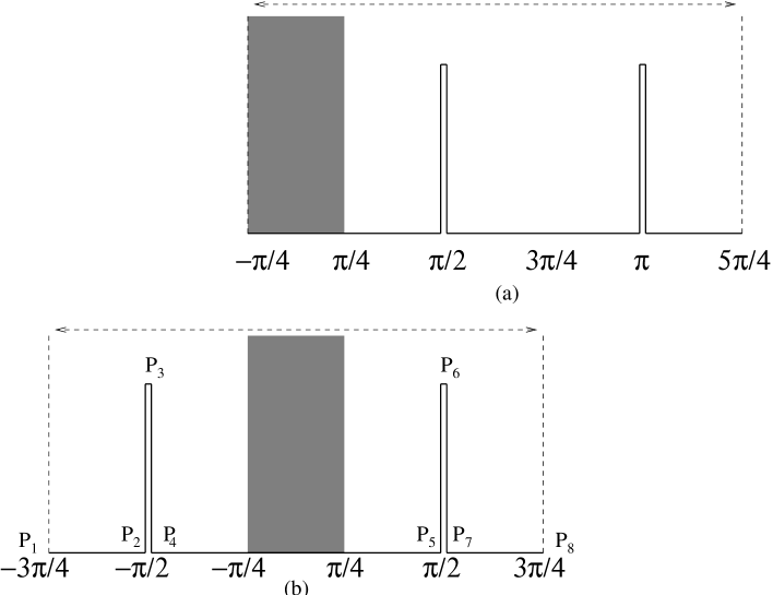
Figure 12: Representation of the $*$-product of a regulated butterfly with itself in the $\widehat{z}$ plane.

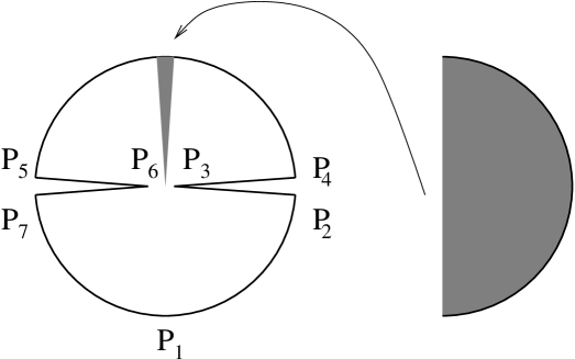
Figure 13: Representation of the $*$-product of a regulated butterfly with itself in the $\widehat{w}$ plane. The local coordinate patch, which is to be glued to the rest of the digram, is shown separately on the right.

To star multiply two regulated butterflies we take the first one, and glue to the right-half of its open string the left-half of the open string of the second butterfly, whose local coordinate patch has been removed. In order to perform these operations it is easier to view the butterfly as the cylinder $-{\pi\over 4}\leq\Re(\widehat{z})\leq{3\pi\over 4},\,\Im(\widehat{z})\geq 0$ with the vertical lines, corresponding to the right half of the open string, identified (see fig. 10(b)). The second (amputated) butterfly can be glued to the right of this one giving the result in fig 12(a). Finally we choose a symmetric arrangement of this figure as shown in figure 12(b). Special points $P_{1},\cdots P_{8}$ have been marked, and the complete picture is a cylinder with circumference ${3\pi/2}$ and with the dashed lines identified. The image of this disk in the $\widehat{w}$ coordinate system is shown in Fig.13. In the $t\to 1$ limit, the vertices $P_{3}$ and $P_{6}$ of the two wedges approach the origin of the $\widehat{w}$ plane, and in this limit the surface clearly has the stucture of a split disk of the form discussed in section 3.1.

Figure 14: The singular points of the map $z\to\widehat{z}$ for the $*$-product of two regulated butterflies in the $z$-plane.

The map of this nontrivial polygon in the $\widehat{z}$ plane into the upper half $z$-plane is defined by a map whose singularity structure is symmetrically arranged as shown in figure 14. Taking into account the various turning points, the map is of the form

$$d\widehat{z}={1\over(1+d^{2}\,z^{2})}\,{(1-b^{2}z^{2})\over\sqrt{(1-a^{2}z^{2})(1-c^{2}z^{2})}}\,dz\equiv H(z)dz\,.$$ (6.11)

The complex poles at $z=\pm{i\over d}$ play no role in the turning points but are needed for the implementation of the identification of the dashed lines in the $\widehat{z}$-plane (figure 12(b)). The length conditions are

$$\displaystyle\int_{0}^{1/a}H(z)dz = {\pi\over 2}\,,$$ (6.12)

$$\int_{1/a}^{1/b}H(z)dz = ih\,,$$ (6.13)

$$\int_{1/b}^{1/c}H(z)dz = -ih\,,$$ (6.14)

$$\int_{1\over c}^{\infty}H(z)dz = {\pi\over 4}\,,$$ (6.15)

where

$$h=\tanh^{-1}t\,.$$ (6.16)

These are four equations, for our four unknowns $a,b,c$ and $d$. These four equations, with the analogous ones integrating over the negative $z$ axis, added together imply that

$$\int_{-\infty}^{\infty}H(z)dz={3\pi\over 2}\,.$$ (6.17)

This means that that the residue around $z={i\over d}$ in (6.11) must equal ${3\over 4i}$. A short calculation shows that this residue condition requires

$${9\over 4}\,d^{2}\,(d^{2}+a^{2})(d^{2}+c^{2})=(d^{2}+b^{2})^{2}\,.$$ (6.18)

It should be noted that this residue condition is not independent from conditions listed in (6.12) to (6.15).

The issue to be examined here is how to achieve very large $h$ by adjusting the parameters $a,b,c$ and $d$. The analysis that follows is a special case of the discussion in section 2.2. As the slits become higher and higher by growing $h$ the surface is pinching. In the representation of Fig.12(a), the role of $R_{2}$ is played by the region ${\pi\over 2}\leq\Re(\widehat{z})\leq\pi$, $\Im(\widehat{z})\geq 0$, which in Fig.12(b) corresponds to the region ${\pi\over 2}\leq|\Re(\widehat{z})|\leq{3\pi\over 4}\,,\Im(\widehat{z})\geq 0$. Our expectation is therefore that as the slits go up to infinity, this region vanishes away in a map that preserves the inner region, and we recover a single butterfly. We will now show that the large $h$ limit can be achieved by taking $b,c$ and $d$ much smaller than $a$, and $c$ to be much smaller than $b,d$:

$$\{b,c,d\}\ll a\,,\qquad c\ll\{b,d\}\,.$$ (6.19)

Since such small parameters imply that the turning points $1/b,1/c$ and $1/d$ are going to infinity, it is convenient to bring them near zero to understand how they are collapsing into each other. We therefore let $z=-1/z^{\prime}$ and find that (6.11) gives

$$d\widehat{z}={1\over(z^{\prime 2}+d^{2})}\,{(z^{\prime 2}-b^{2})\over\sqrt{(z^{\prime 2}-a^{2})(z^{\prime 2}-c^{2})}}\,dz^{\prime}\equiv G(z^{\prime})dz^{\prime}\,.$$ (6.20)

Our first condition will be to achieve (6.12). This gives

$$\int_{a}^{\infty}G(z^{\prime})dz^{\prime}\simeq\int_{a}^{\infty}{dz^{\prime}\over z^{\prime}}{1\over\sqrt{z^{\prime 2}-a^{2}}}={\pi\over 2}\,,$$ (6.21)

where we have noted in (6.20) that for $a<z^{\prime}<\infty$ and the inequalities in (6.19), $z^{\prime}\gg b,c,d$, and the expression for $G(z^{\prime})$ simplifies considerably. This equation requires

$$a\simeq 1\,.$$ (6.22)

With $a\simeq 1$ and much bigger than $b,c$ and $d$, and $c$ much smaller than $b$, $d$, equation (6.18) now gives

$${1\over 2}\,d^{2}\simeq b^{2}\,.$$ (6.23)

With $d$ comparable to $b$, and $c\ll\{d,b\}$ we now claim that all the conditions listed in (6.12) to (6.15), and the demand that $h$ be large, can be satisfied. Since (6.18) and thus (6.23) is a consequence of (6.12) and (6.15), and we have already satisfied (6.12), we should be able to see that (6.15) is satisfied. Indeed, we must have

$$\int_{0}^{c}G(z^{\prime})dz^{\prime}\simeq\int_{0}^{c}{b^{2}\over d^{2}\sqrt{c^{2}-z^{\prime 2}}}dz^{\prime}\simeq{\pi\over 4}\,.$$ (6.24)

A short calculation shows that this equation holds on accound of (6.23).

It only remains now to verify that conditions (6.13) and (6.14) can be satisfied with ever increasing $h$. Condition(6.13) requires that the integral

$$\int_{b}^{1}{1\over z^{\prime 2}+2b^{2}}\,{z^{\prime 2}-b^{2}\over\sqrt{1-z^{\prime 2}}}\,{dz^{\prime}\over z^{\prime}}\,$$ (6.25)

obtained using (6.19) grow without bounds as $b$ is made progressively small. This is clearly the case, since the integral diverges at the bottom limit when $b$ is set to zero. This means that for any $h$ we can satisfy (6.13) for sufficiently small $b$, with $c\ll b$. Condition (6.14) requires that the integral

$$\int_{c}^{b}{dz^{\prime}\over z^{\prime 2}+2b^{2}}\,{z^{\prime 2}-b^{2}\over\sqrt{z^{\prime 2}-c^{2}}}\,\,$$ (6.26)

obtained using (6.19), grow without bounds as $c$ is made progressively small. This is clearly the case, since the integral diverges at the bottom limit when $c$ is set to zero. This means that having satisfied (6.13) for a fixed and very large $h$ by choosing a sufficiently small $b$ while keeping $c\ll b$, we can now satisfy (6.14) by making $c$ sufficiently small.

We have thus shown that as we multiply two regulated butterflies and let the regulator go away, the map defining the composite surface is that of (6.11), with the limit $a\to 1$, and $\{b,c,d\}\to 0$ taken. This gives us

$$d\widehat{z}=\,{1\over\sqrt{1-z^{2}}}\,dz\,,$$ (6.27)

which, by comparison to (6.5), it is immediately recognized to be the definition of the butterfly. This concludes our proof that the butterfly emerges from the star product of two regulated butterflies in the limit as the regulator is removed.

It is natural to wonder if the multiplication of two regulated butterflies also gives a regulated butterfly for $t\simeq 1$. We find that this product is a butterfly regulated in a slightly different way. To see this note that using (6.23), we can go back to (6.18) to find a more accurate evaluation of $a$, which previously was just set to one. We find

$$d^{2}\simeq 1-a^{2}\,.$$ (6.28)

With such relation, the map (6.11) becomes

$$d\widehat{z}={1\over(1+(1-a^{2})\,z^{2})}\,{(1-{1\over 2}(1-a^{2})z^{2})\over\sqrt{1-a^{2}z^{2}}}\,dz\,,$$ (6.29)

where we used $c\ll\{b,d\}$. The correspondence with the regulated butterfly map given in (6.7) is very close, but not exact. The reason for this is intuitively clear. Our conformal map statement in section 3.1 states that the map that shrinks away the extra surface at the other side of a thin neck only affects the region around this neck. In addition, regulators control the approach of the boundary to the open string midpoint. Since the neck arising from star multiplication occurs around the open string midpoint of the product string (see, for example fig. 8), the regulator arising after star product is affected by the way in which the map shrinks away the extra surface.

6.4 Half-string wave-functional for the butterfly state

Figure 15: The $\widehat{\cal R}_{1/2}$ associated with the butterfly state, and its images under the maps $h^{-1}$, $s\circ h^{-1}$ and $h\circ s\circ h^{-1}$. $P$ and $Q$ are two marked points on the boundary of the disk, and the labels $P$ and $Q$ are always located in the inside of the disk.

Figure 16: The $\widehat{\Sigma}_{1/2}$ associated with the butterfly.

According to the general arguments given in section 4.1, the wave-functional of the butterfly state splits into a product of a functional of the left half of the string and a functional of the right half of the string. We can now ask: what particular half-string wave-functional does the butterfly state have? To answer this question we go back to eq.(4.14). In the case of the butterfly, $\widehat{\cal R}_{top}$ is the unit quarter disk in the second quadrant as shown in the top left hand diagram of Fig.15. As shown in the rest of the figure, under the map $h\circ s\circ h^{-1}$ this gets mapped to the unit half-disk to the left of the vertical axis. This then is the $\widehat{\cal R}_{1/2}$ for the butterfly. Thus the disk $\widehat{\Sigma}_{1/2}$, obtained by joining with $\widehat{\cal R}_{1/2}$ the copy of the local coordinate patch, is the full unit disk as shown in Fig.16. This gives the half string state associated with the butterfly to be:

$$|\Phi\rangle=|0\rangle\,,$$ (6.30)

thereby establishing that the half-string wave-functional associated with the butterfly state is the vacuum state.

6.5 Operator representation of the butterfly state

We can represent the regulated butterfly $|{\cal B}_{t}\rangle$ in the operator formalism following the general procedure outlined in section 2.3. In this case we have

$$z=f_{t}(\xi)=\frac{\xi}{\sqrt{1+t^{2}\xi^{2}}}=\exp\Bigl{(}v_{t}(\xi){\partial\over\partial\xi}\Bigr{)}\,\xi\,.$$ (6.31)

Eqs.(2.18), (2.17) give

$$v_{t}(\xi)=-t^{2}\,\xi^{3}/2\,.$$ (6.32)

Eq.(2.11), (2.13) now gives:

$$|{\cal B}_{\,t}\rangle=\exp\left(-\frac{t^{2}}{2}\,L_{-2}\right)|0\rangle\,.$$ (6.33)

This is a remarkably simple expression involving a single Virasoro operator in the exponent.

The formalism of Virasoro conservation laws [32] allows us to derive an interesting property of the butterfly state,

$$K_{2}|{\cal B}\rangle=0\,,$$ (6.34)

where $K_{2}=L_{2}-L_{-2}$. Indeed, consider in the global UHP the vector field

$$\tilde{v}_{2}(z)=2z-\frac{1}{z}\,,$$ (6.35)

which is holomorphic everywhere, including infinity, except for the pole at the puncture $z=0$. It follows that

$$\Big{\langle}\oint dz\;\tilde{T}(z)\,\tilde{v}_{2}(z)f_{{\cal B}}\circ\phi(0)\Big{\rangle}_{UHP}=0\,,$$ (6.36)

for any state $|\phi\rangle$, where the contour circles the origin. Changing variables to the local coordinate $\xi$, we find

$$\Big{\langle}f_{{\cal B}}\circ\Big{(}\oint d\xi\;T(\xi)(\xi^{3}-\xi^{-1})\phi(0)\Big{)}\Big{\rangle}_{UHP}=0\,.$$ (6.37)

This gives

$$\langle{\cal B}|K_{2}|\phi\rangle=0$$ (6.38)

since $\langle{\cal B}|\chi\rangle=\langle f_{{\cal B}}\circ\chi(0)\rangle$ for any state $|\chi\rangle$. This, in turn, is equivalent to (6.34).

6.6 Oscillator representation of the butterfly state

We can also represent the matter part of the regulated butterfly state in the oscillator representation using eq.(2.19), (2.23). In this case, with $\beta\equiv t^{2}$,

$$v(\xi)=-\frac{\xi^{3}}{2}\,,\qquad f_{\beta}(\xi)=\frac{\xi}{\sqrt{1+\beta\xi^{2}}}\,.$$ (6.39)

Equ. (2.23) gives

$$\displaystyle\frac{d}{d\beta}V_{mn}(\beta) = (-1)^{m+n}\frac{\sqrt{mn}}{2}\oint_{0}{dw\over 2\pi i}\oint_{0}{dz\over 2\pi i}\,{1\over z^{m+1}w^{n+1}}\frac{f_{\beta}(z)^{3}-f_{\beta}(w)^{3}}{f_{\beta}(z)-f_{\beta}(w)}$$

$$= (-1)^{m+n}\frac{\sqrt{mn}}{2}\oint_{0}{dw\over 2\pi i}\frac{f_{\beta}(w)}{w^{m+1}}\oint_{0}{dz\over 2\pi i}\frac{f_{\beta}(z)}{z^{m+1}}=(-1)^{m+n}\frac{\sqrt{mn}}{2}\,x_{m}x_{n}\,,$$

where

$$\displaystyle x_{m}=\oint_{0}{dw\over 2\pi i}\frac{f_{\beta}(w)}{w^{m+1}} = (-\beta)^{\frac{m-1}{2}}\frac{\Gamma[\frac{m}{2}]}{\sqrt{\pi}\Gamma[\frac{m+1}{2}]}\quad{\rm for}\;m\;{\rm odd}\,,$$

$$= 0\quad\qquad\qquad\qquad\qquad{\rm for}\;m\;{\rm even}\,.$$

Integrating (6.6) with the initial condition $V(\beta=0)=0$, we find the Neumann coefficients of the regulated butterfly $(\beta\to t^{2})$:

$$\displaystyle V_{mn}(t) = -(-1)^{\frac{m+n}{2}}\frac{\sqrt{mn}}{m+n}\frac{\Gamma[\frac{m}{2}]\Gamma[\frac{n}{2}]}{\pi\Gamma[\frac{m+1}{2}]\Gamma[\frac{n+1}{2}]}\,t^{m+n}\,,\quad{\rm for}\;m\;{\rm and}\;n\;{\rm odd}\,,$$

$$= 0\,,\qquad\qquad\qquad\qquad\qquad\qquad\qquad\quad\quad\;\;\quad{\rm for}\;m\;{\rm or}\;n\;{\rm even}\,.$$

7 The Nothing State

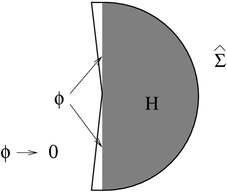
Figure 17: The geometry of the disk $\widehat{\Sigma}$ for the nothing state. Since the local coordinate patch fills the whole disk, the region $\widehat{\cal R}$, which represents the full disk $\widehat{\Sigma}$ minus the local coordinate patch, collapses to nothing.

The nothing state is defined by the relation:

$$\langle{\cal N}|\phi\rangle=\langle f_{\cal N}\circ\phi(0)\rangle_{UHP}\,,$$ (7.1)

with

$$f_{\cal N}(\xi)={\xi\over\xi^{2}+1}\,.$$ (7.2)

Under the map $\widehat{w}(\xi)=h(\xi)$ with $h(\xi)$ defined as in eq.(2.5), the upper half $z=f_{\cal N}(\xi)$ plane gets mapped to the vertical half-disk $\widehat{\Sigma}$ as shown in Fig.17. Clearly the boundary along the vertical line passes through the string mid-point which is at the origin of the $\widehat{w}$-plane, and hence this state satisfies the usual criterion of being a projector of the $*$-algebra.

Various properties of the nothing state can be derived along the same lines as those of the butterfly. Here we summarize the main results:

• The nothing state factorizes into a product of the nothing state for the left half-string and the nothing state for the right half-string. This follows from the results of section 4.2, – since in this case $\widehat{\cal R}$ associated with the original projector collapses, $\widehat{\cal R}_{top}$ also collapses and hence from (4.14) it follows that $\widehat{\cal R}_{1/2}$ also collapses. Thus $\widehat{\Sigma}_{1/2}$ is identical to $\widehat{\Sigma}$. This proves that the half-string state is the same as the original state.

• The map $f_{{\cal N}}(\xi)$ defining the nothing state is related to the map $f_{{\cal I}}(\xi)$ defining the identity string field by

  $$f_{{\cal N}}(\xi)=-if_{{\cal I}}(i\xi)\,.$$ (7.3)

  It follows from (2.11)–(2.13) that the operator expressions of the identity and of the nothing state are related by the formal replacement $L_{-2n}\leftrightarrow(-)^{n}L_{-2n}$. The identity admits an elegant operator expression [41] as an infinite product of exponentials of Virasoro generators. Changing the sign of $L_{-2}$ in (3.3) of [41], we immediately have

  $$\displaystyle|{\cal N}\rangle = \left(\prod\limits_{n=2}^{\infty}\exp\left\{-\frac{2}{2^{n}}L_{-2^{n}}\right\}\right)e^{-L_{-2}}|0\rangle$$ (7.4)

  $$= \ldots\exp(-\frac{2}{2^{3}}L_{-2^{3}})\exp(-\frac{2}{2^{2}}L_{-2^{2}})\exp(-L_{-2})|0\rangle\,.$$

• $V^{f}_{mn}$ computed using (2.20), (7.2) turns out to be equal to $\delta_{mn}$. Thus the oscillator representation of the matter part of the nothing state is given by:

  $$|{\cal N}\rangle_{m}=\exp\left(-\frac{1}{2}\sum_{m,n=1}^{\infty}a^{\dagger}_{n}a^{\dagger}_{n}\right)|0\rangle\,.$$ (7.5)

• Computation of $A_{f}$ following eq.(2.28) gives $A_{f}=0$. Using eq.(2.25) we then see that the wave-functional of the nothing state, expressed as a functional of the coordinates $X_{n}$, is a constant independent of $X_{n}$.

• The nothing state is annihilated by all even reparametrizations of the cubic vertex,

  $$K_{2n}|{\cal N}\rangle=0\qquad\forall n\,,$$ (7.6)

  where $K_{2n}=L_{2n}-L_{-2n}$. This is shown with an argument similar to the one used for the butterfly state, eqs.(6.34)-(6.38). Taking in this case the globally-defined vector fields

  $$\tilde{v}_{2}(z)=-\frac{1}{z}+4z\,,\quad\tilde{v}_{4}(z)=-\frac{1}{z^{3}}+\frac{6}{z}-8z\,,$$ (7.7)

  we find that

  $$K_{2}|{\cal N}\rangle=0\,,\quad K_{4}|{\cal N}\rangle=0\,.$$ (7.8)

  The commutation relations

  $$[K_{m}\,,K_{n}]=(m-n)K_{m+n}-(-1)^{n}(m+n)K_{m-n}$$ (7.9)

  then imply (7.6) for all $n$. Let us recall that the identity string field is annihilated by all, even and odd, vertex reparametrizations [32], so from this point of view the nothing state is the most symmetric surface state apart from the identity.

8 The Generalized Butterfly States

In this section we shall introduce a new class of surface states, $-$ called generalized butterflies, $-$ each of which is a projector of the star algebra. We shall first define these states, and then show that each of these states satisfies the projector equation. We shall also determine the half-string wave-functionals that the wave-functional of the generalized butterfly state factorizes into.

8.1 Definition of general butterflies

Let us begin by defining the generalized butterfly state $|{\cal B}_{\alpha}\rangle$. We generalize eq.(6.1) to

$$z={1\over\alpha}\sin(\alpha\tan^{-1}\xi)\equiv f_{\alpha}(\xi)\,.$$ (8.1)

As a result eq.(6.3) is generalized to

$$z={1\over\alpha}\sin(\alpha\widehat{z})\,.$$ (8.2)

Comparing eqs.(6.3) and (8.2) we see that the generalized butterfly differs from the original butterfly by a rescaling of the $\widehat{z}$ coordinate by a factor $\alpha$. Having a look at figure 9(c), we see that the generalized butterfly occupies the region $-{\pi\over 2\alpha}<\Re(\widehat{z})\leq{\pi\over 2\alpha}$ in the upper half $\widehat{z}$ plane. We denote by ${\cal C}_{\alpha}$ this region in the $\widehat{z}$ coordinate system, or more precisely, a convenient translate of it.

As can be easily seen from eq.(8.1), the map $f_{\alpha}(\xi)$ is singular at the string mid-point $\xi=i$. In particular the mid-point is sent to $i\infty$ and hence touches the boundary of the upper half $z$-plane. Thus from the general analysis of section 4 we expect these states to be projectors of the $*$-algebra and have factorized wave-functionals. Also note that we have:

$$f_{\alpha=1}={\xi\over\sqrt{1+\xi^{2}}}\,.$$ (8.3)

Comparison with eq.(6.1) shows that the state $|{\cal B}_{\alpha=1}\rangle$ is identical to the butterfly state defined in the previous section. On the other hand, we have:

$$f_{\alpha=0}=\tan^{-1}\xi\,.$$ (8.4)

This shows that the state $|{\cal B}_{\alpha=0}\rangle$ is identical to the sliver. The family of surface states $|{\cal B}_{\alpha}\rangle$ gives a family of projectors, interpolating between the butterfly and the sliver. Finally, note that for $\alpha=2$ we have the map

$$f_{\alpha=2}={\xi\over 1+\xi^{2}}\,.$$ (8.5)

For reasons to be explained shortly, we call this the ‘nothing’ state.

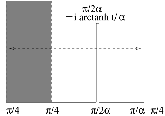
Figure 18: The geometry of ${\cal C}_{\alpha,t}$ in the complex $\widehat{z}$ plane. The shaded region denotes the local coordinate patch, and the lines $\Re(\widehat{z})=-\pi/4$, $\Re(\widehat{z})=\pi/\alpha-\pi/4$ are identified.

We can regularize the singularity at the midpoint and define the regularized butterfly by generalizing (6.9) to

$$z=f_{\alpha,t}(\xi)={1\over\alpha}{\tan(\alpha\tan^{-1}\xi)\over\sqrt{1+t^{2}\tan^{2}(\alpha\tan^{-1}\xi)}}={1\over\alpha}{\tan(\alpha\widehat{z})\over\sqrt{1+t^{2}\tan^{2}(\alpha\widehat{z})}}\,.$$ (8.6)

In the $\widehat{z}$ plane we get

$$\langle{\cal B}_{\alpha,t}|\phi\rangle=\langle f^{(0)}\circ\phi(0)\rangle_{{\cal C}_{\alpha,t}}\,,$$ (8.7)

where ${\cal C}_{\alpha,t}$ is the image of the upper half $z$ plane in the $\widehat{z}$ coordinate system and $f^{(0)}(\xi)=\tan^{-1}\xi$. Comparison between (6.9) and (8.6) shows that the regularized butterfly and the regularized generalized butterfly are related by a rescaling of the $\widehat{z}$ coordinate by $1/\alpha$. Thus ${\cal C}_{\alpha,t}$ can be obtained by a rescaling of Fig.10(a) by $1/\alpha$, and moving the region to the left of the coordinate patch all the way to the right, as shown in Fig.18. Note that the local coordinate patch always occupies the same region $|\Re(\widehat{z})|\leq{\pi\over 4}$, $\Im(\widehat{z})\geq 0$, since $\widehat{z}=\tan^{-1}\xi$.

As shown, ${\cal C}_{\alpha,t}$ is a semi-infinite cylinder with circumference $\pi/\alpha$, obtained by the restriction $\Im(\widehat{z})\geq 0$, $-\pi/4\leq\Re(\widehat{z})\leq\pi/\alpha-\pi/4$, and the identification $\Re(\widehat{z})=\Re(\widehat{z})+\pi/\alpha$ in the $\widehat{z}$ plane, with a cut along the line $\Re(\widehat{z})=\pi/2\alpha$, extending all the way from the base $\widehat{z}=\pi/2\alpha$ to $\widehat{z}=\pi/2\alpha+i(\tanh^{-1}t)/\alpha$. As we move along the real $z$ axis, in the $\widehat{z}$ plane we go from $\widehat{z}=-\pi/4$ to $\pi/2\alpha$ along the real axis, then along the cut to $\pi/2\alpha+i(\tanh^{-1}t)/\alpha$ and back to $\pi/2\alpha$, and finally along the real axis to $-\pi/4+\pi/\alpha$. The local coordinate patch, corresponding to the unit half-disk in the upper half $\xi$ plane, is mapped to the semi-infinite strip $\Im(\widehat{z})\geq 0$, $-\pi/4\leq\Re(\widehat{z})\leq\pi/4$. The lines $\Re(\widehat{z})=\pi/4$ and $\Re(\widehat{z})=\pi/\alpha-\pi/4\equiv-\pi/4$ correspond to the images of the left and the right half of the string respectively. As $t\to 1$ the cut goes all the way to $\pi/2\alpha+i\infty$. The image of ${\cal C}_{\alpha,t}$ in the complex $\widehat{w}=e^{2i\widehat{z}}$ plane in the $t\to 1$ limit has been shown in Fig.19.

The tip of the cut at $\widehat{z}=\pi/2\alpha+i(\tanh^{-1}t)/\alpha$ corresponds to the branch point coming from the square root in the denominator of (8.6). According to our convention we choose the positive sign of the square root to the left of this cut, $-$ this forces us to choose the negative sign to the right of the cut. Thus in the $t\to 1$ limit, the map from the $z$-plane to the $\widehat{z}$ plane takes the form:

$$\displaystyle z=f_{\alpha,t=1}(\xi) = {1\over\alpha}\sin(\alpha\widehat{z})\qquad\hbox{for}\quad\Re(\widehat{z})<\pi/2\alpha\,,$$ (8.8)

$$= -{1\over\alpha}\sin(\alpha\widehat{z})\qquad\hbox{for}\quad\Re(\widehat{z})>\pi/2\alpha\,.$$

The difference from (8.2) for $\Re(\widehat{z})>\pi/2\alpha$ arises because we redefined asymmetrically the fundamental domain in the $\widehat{z}$ plane. Note that for $\alpha=2$ the region of ${\cal C}_{\alpha,t}$ outside the local coordinate patch collapses to nothing. For this reason we call the associated surface state the ‘nothing’ state.

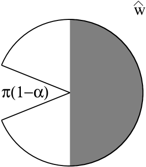
Figure 19: The image of ${\cal C}_{\alpha}$ in the complex $\widehat{w}=e^{2i\widehat{z}}$ plane. The shaded region denotes the local coordinate patch.

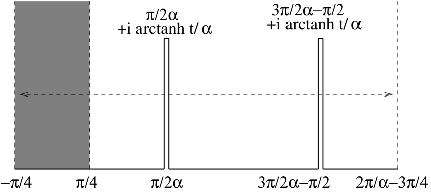
Figure 20: The geometry of ${\cal C}^{\prime}_{\alpha,t}$ in the complex $\widehat{z}$ plane. The shaded region denotes the local coordinate patch, and the lines $\Re(\widehat{z})=-\pi/4$, $\Re(\widehat{z})=2\pi/\alpha-3\pi/4$ are identified.

8.2 Squaring the generalized butterfly

We now want to show that $|{\cal B}_{\alpha}\rangle$ squares to itself under $*$ product. For this we shall first compute $|{\cal B}_{\alpha,t}*{\cal B}_{\alpha,t}\rangle$, and then take the $t\to 1$ limit. Throughout this section we shall work in the combined matter-ghost system with zero central charge so that we can apply the gluing theorem without any additional factors coming from conformal anomaly. Since the discussion proceeds in a manner closely parallel to that in section 6.3, we shall omit the details and only point out the essential differences.

As in section 6.3, we work in the $\widehat{z}$ coordinates. We begin with two copies of ${\cal C}_{\alpha,t}$ (one for each ${\cal B}_{\alpha,t}$), simply remove the local coordinate patch from the second ${\cal C}_{\alpha,t}$ and glue the image of the right half string on the first ${\cal C}_{\alpha,t}$ with the image of the left half string on the second ${\cal C}_{\alpha,t}$. The result is a cylinder ${\cal C}^{\prime}_{\alpha,t}$ of circumference

$${2\pi\over\alpha}-{\pi\over 2}\,,$$ (8.9)

defined as the region $\Im(\widehat{z})\geq 0$, $-\pi/4\leq\Re(\widehat{z})\leq 2\pi/\alpha-3\pi/4$. It also has two cuts, one along the line $\Re(\widehat{z})=\pi/2\alpha$, extending from $\widehat{z}=\pi/2\alpha$ to $\widehat{z}=\pi/2\alpha+i(\tanh^{-1}t)/\alpha$, and the other along the line $\Re(\widehat{z})=3\pi/2\alpha-\pi/2$, extending from $\widehat{z}=3\pi/2\alpha-\pi/2$ to $\widehat{z}=3\pi/2\alpha-\pi/2+i(\tanh^{-1}t)/\alpha$. The local coordinate patch on ${\cal C}^{\prime}_{\alpha,t}$ is the vertical strip bounded by the lines $\Re(\widehat{z})=\pm\pi/4$. This has been shown in Fig.20.

Let $z=F_{\alpha,t}(\widehat{z})$ describes the map of ${\cal C}^{\prime}_{\alpha,t}$ to UHP. In order to show that ${\cal B}_{\alpha}$ squares to itself, we need to show that as $t\to 1$, the map $F_{\alpha,t}(\widehat{z})$ approaches the map given in (8.2) in the vicinity of the origin. Thus the task is now to determine the map $F_{\alpha,t}$ that maps the $\widehat{z}$ plane to the upper half plane labeled by the coordinate $z$. It is defined implicitly through the differential equation analogous to (6.11):

$$d\widehat{z}={1\over(1+d^{2}\,z^{2})}\,{(1-b^{2}z^{2})\over\sqrt{(1-a^{2}z^{2})(1-c^{2}z^{2})}}\,dz\equiv H(z)dz\,.$$ (8.10)

The analog of eqs.(6.12)-(6.15) are:

$$\displaystyle\int_{0}^{1/a}H(z)dz = {\pi\over 2\alpha}\,,$$ (8.11)

$$\int_{1/a}^{1/b}H(z)dz = ih/\alpha\,,$$ (8.12)

$$\int_{1/b}^{1/c}H(z)dz = -ih/\alpha\,,$$ (8.13)

$$\int_{1\over c}^{\infty}H(z)dz = {\pi\over 2\alpha}-{\pi\over 4}\,,$$ (8.14)

with $h$ as defined in eq.(6.16).

In the $t\to 1$ limit the height $h$ of the cylinder goes to $\infty$. We shall now show that this can be achieved by taking

$$\{b,c,d\}\ll a,\qquad c\ll\{b,d\}\,.$$ (8.15)

As in section 6.3 we define $z\to-1/z^{\prime}$ and rewrite (8.10) as

$$d\widehat{z}={1\over(z^{\prime 2}+d^{2})}\,{(z^{\prime 2}-b^{2})\over\sqrt{(z^{\prime 2}-a^{2})(z^{\prime 2}-c^{2})}}\,dz^{\prime}=G(z^{\prime})dz^{\prime}\,.$$ (8.16)

In the limit $\{b,c,d\}\ll a$, (8.11) gives:

$$\int_{a}^{\infty}G(z^{\prime})dz^{\prime}\simeq\int_{a}^{\infty}{dz^{\prime}\over z^{\prime}}{1\over\sqrt{z^{\prime 2}-a^{2}}}={\pi\over 2\alpha}\,.$$ (8.17)

This requires

$$a\simeq\alpha\,.$$ (8.18)

Proceeding as in the case of section 6.3, we can now show that all the other conditions (8.12)-(8.14), and the requirement of large $h$ can be satisfied by taking:

$$c\ll b,d,\qquad d\sim b\,.$$ (8.19)

Using eqs.(8.15) and (8.18), we see that eq.(8.10) now takes the form:

$$d\widehat{z}=\,{1\over\sqrt{1-\alpha^{2}z^{2}}}\,dz\,,$$ (8.20)

which gives:

$$z={1\over\alpha}\sin(\alpha\widehat{z})\,.$$ (8.21)

This is precisely the map for the generalized butterfly. This establishes that the generalized butterfly squares to itself under $*$-product.

8.3 Wave-functionals for generalized butterfly states

In this subsection we shall apply the general method described in section 2.5 to compute the wave-functional of the generalized butterfly state. In this process, we shall show explicitly that the wave-functional factorizes into a product of a functional of the left-half of the string and a functional of the right-half of the string. The wave-functional of the butterfly state is expressed as

$$\langle{\cal B}_{\alpha}|X\rangle={\cal N}_{{\cal B}_{\alpha}}\exp\left(-\frac{1}{2}\int_{0}^{\pi}\int_{0}^{\pi}d\sigma d\sigma^{\prime}X(\sigma)A_{{\cal B}_{\alpha}}(\sigma,\sigma^{\prime})X(\sigma^{\prime})\right)\,.$$ (8.22)

Figure 21: The geometry involved in the computation of the inner product of two generalized butterflies in the $\widehat{z}$-plane.

As seen from eqs.(2.29) and (2.30), computation of $A_{{\cal B}_{\alpha}}(\sigma_{1},\sigma_{2})$ defined in eq.(8.22) requires computing correlation functions of the form $\langle{\cal B}_{\alpha,t}|\cdots|{\cal B}_{\alpha,t}\rangle$, and then taking the limit $t\to 1$. To do this computation one simply removes the local coordinate patch from each ${\cal C}_{\alpha,t}$ and glues the left half of one with the right half of the other and vice versa. The result is a semiinfinite cylinder ${\cal C}^{\prime\prime}_{\alpha,t}$ of circumference $(2\pi/\alpha-\pi)$, corresponding to the region $\Im(\widehat{z})\geq 0$, $\pi/4\leq\Re(\widehat{z})\leq\pi/4+2\pi/\alpha-\pi$, with the identification $\widehat{z}\equiv\widehat{z}+(2\pi/\alpha-\pi)$, and with two vertical cuts, one going from $\widehat{z}=\pi/2\alpha$ to $\widehat{z}=\pi/2\alpha+i(\tanh^{-1}t)/\alpha$, and the other going from $\widehat{z}=3\pi/2\alpha-\pi/2$ to $\widehat{z}=3\pi/2\alpha-\pi/2+i(\tanh^{-1}t)/\alpha$ respectively. The two halves of the string along which we have glued the two copies of ${\cal C}_{\alpha,t}$ to produce the cylinder ${\cal C}^{\prime\prime}_{\alpha,t}$ lie along the lines $\Re(\widehat{z})=\pi/4$ and $\pi/\alpha-\pi/4$ respectively. This has been shown in Fig.21. Thus we have, using (2.29) and (2.30):

$${1\over 2}\partial_{\sigma_{1}}\partial_{\sigma_{2}}A_{{\cal B}_{\alpha}}^{-1}(\sigma_{1},\sigma_{2})=\partial_{\sigma_{1}}\partial_{\sigma_{2}}\langle X(\widehat{z}_{1})X(\widehat{z}_{2})\rangle_{{\cal C}^{\prime\prime}_{\alpha,t}}\,.$$ (8.23)

This correlation function can be calculated by finding the conformal transformation that maps the cylinder ${\cal C}^{\prime\prime}_{\alpha,t}$ to the upper half plane, and re-expressing (8.23) as a correlation function on the upper half plane. This gives

$$\displaystyle{1\over 2}\partial_{\sigma_{1}}\partial_{\sigma_{2}}A_{{\cal B}_{\alpha}}^{-1}(\sigma_{1},\sigma_{2}) = \partial_{\sigma_{1}}\partial_{\sigma_{2}}\langle X(z_{1})X(z_{2})\rangle_{UHP}$$ (8.24)

$$= -{1\over 2}\partial_{\sigma_{1}}\partial_{\sigma_{2}}\{\ln|z_{1}-z_{2}|^{2}+\ln|z_{1}-\bar{z}_{2}|^{2}\}\,,$$

with $z_{i}$’s computed in terms of $\sigma_{i}$’s with the help of the map that relates $\widehat{z}=\tan^{-1}\xi=\tan^{-1}(e^{i\sigma})$ to the upper half plane coordinate $z$. We could proceed as in section 8.2 to construct the map from the $\widehat{z}$ plane to the $z$-plane, but in this case we can write down a closed form expression for this map. The function that maps ${\cal C}^{\prime\prime}_{\alpha,t}$ in the $\widehat{z}$ coordinate to the upper half plane labeled by $z$ is given by:

$$z=g_{\alpha,t}(\xi)=g_{\alpha,t}(\tan\widehat{z})$$ (8.25)

with

$$g_{\alpha,t}(\xi)=\sqrt{\tan^{2}(\beta\tan^{-1}\xi+\gamma)+u^{2}\over 1+u^{2}\tan^{2}(\beta\tan^{-1}\xi+\gamma)}=\sqrt{\tan^{2}(\beta\widehat{z}+\gamma)+u^{2}\over 1+u^{2}\tan^{2}(\beta\widehat{z}+\gamma)}$$ (8.26)

where

$${1\over\beta}={2\over\alpha}-1,\qquad\gamma={\pi\over 2}(1-{\beta\over\alpha}),\qquad{1\over\beta}\tanh^{-1}u={1\over\alpha}\tanh^{-1}t\,.$$ (8.27)

To see that this maps ${\cal C}^{\prime\prime}_{\alpha,t}$ to the upper half plane, we can start from $\widehat{z}=\pi/4$ and follow the boundary of ${\cal C}^{\prime\prime}_{\alpha,t}$ to see that it maps to the real line in the $z$ plane. As we start from $\widehat{z}=\pi/4$ and travel along the real axis to $\widehat{z}=\pi/2\alpha$, $z$ travels along the real line from 1 to $1/u$ As $\widehat{z}$ goes from the point $\widehat{z}=\pi/2\alpha$ towards $\pi/2\alpha+i(\tanh^{-1}t)/\alpha$, $z$ goes from $1/u$ to $\infty$. Then as $\widehat{z}$ returns back to $\pi/2\alpha$ along the same line, $z$ goes from $-\infty$ to $-1/u$, and as $\widehat{z}$ travels along the real axis to $\widehat{z}=(3\pi/2\alpha-\pi/2)$, $z$ goes from $-1/u$ to $-u$, passing through $-1$ at $\widehat{z}=(\pi/\alpha-\pi/4)$. As $\widehat{z}$ travels along the vertical line from $\widehat{z}=(3\pi/2\alpha-\pi/2)$ to $\widehat{z}=(3\pi/2\alpha-\pi/2)+i(\tanh^{-1}t)/\alpha$, $z$ goes from $-u$ to 0, and as we return back to the point $\widehat{z}=3\pi/2\alpha-\pi/2$ along the same line, $z$ goes from 0 to $u$. Finally, as we move from $\widehat{z}=(3\pi/2\alpha-\pi/2)$ to $\widehat{z}=(\pi/4+2\pi/\alpha-\pi)$, $z$ goes from $u$ to 1. Since in the $\widehat{z}$ plane we identify the lines $\Re(\widehat{z})=(\pi/4+2\pi/\alpha-\pi)$ with $\Re(\widehat{z})=\pi/4$, the contour closes.

From the map of the boundary to the real $z$ axis described above we see that the ends of the half strings, $\widehat{z}=\pi/4$ and $\widehat{z}=(\pi/\alpha-\pi/4)$ maps to $1$ and $-1$ respectively. From eqs.(8.25), (8.26), (8.27) we see that the half string $\Re(\widehat{z})=\pi/4$ gets mapped to

$$z=\sqrt{(1+iS)^{2}+u^{2}(1-iS)^{2}\over(1-iS)^{2}+u^{2}(1+iS)^{2}}\,,$$ (8.28)

where

$$S=\tanh(\beta\Im(\widehat{z}))\,.$$ (8.29)

On the other hand the half-string $\Re(\widehat{z})=(\pi/\alpha-\pi/4)$ gets mapped to

$$z=-\sqrt{(1-iS)^{2}+u^{2}(1+iS)^{2}\over(1+iS)^{2}+u^{2}(1-iS)^{2}}\,.$$ (8.30)

From eq.(8.27) we see that as $t\to 1$ we have $u\to 1$. Eqs.(8.28) and (8.30) then show that as $u\to 1$, the left and right half-strings are mapped in such a way that all points of the left one, and all points on the right one, except for the one associated to the full string midpoint, approach the points $1$ and $-1$ respectively. The half strings remain infinite in the $z$ plane but are being reparametrized so that all of their inner points are approaching either $1$ or $-1$. Eq.(8.24) now gives

$${1\over 2}\partial_{\sigma_{1}}\partial_{\sigma_{2}}A_{{\cal B}_{\alpha}}^{-1}(\sigma_{1},\sigma_{2})=0\,\qquad\hbox{if}\quad 0\leq\sigma_{1}<\pi/2,\quad\pi/2<\sigma_{2}\leq\pi\,.$$ (8.31)

Indeed, since the half-string points $\sigma_{1}$ and $\sigma_{2}$ are mapped to fixed points in the limit $t\to 1$, the derivatives $dz_{i}/d\sigma_{i}$ go to zero, and with $|z_{1}-z_{2}|$ finite, the evaluation of the right hand side of Eq.(8.24) gives zero. This is consistent with the wave-functional factorizing into a product of a functional of the left half-string and a functional of the right half-string. Indeed, since the interior of the right half-string is going into a point and the interior of the left half-string is going into another point in the $z$-plane, we have an explicit verification of the factorization relation (4.3).

In order to determine which particular state of the half-string appears in the product, we need to evaluate the right hand side of (8.24) when $\sigma_{1}$ and $\sigma_{2}$ lie on the same half of the string. For definiteness we shall take $0\leq\sigma_{1},\sigma_{2}<\pi/2$. The coordinate $\sigma$ of the half-string is related to $\widehat{z}$ through $\widehat{z}=\tan^{-1}(e^{i\sigma})$. On the left half string, we can rewrite this as:

$$\widehat{z}=\pi/4+{i\over 2}\ln\bigg{(}{1+\sin\sigma\over\cos\sigma}\bigg{)}\,.$$ (8.32)

Using eqs.(8.29), (8.32) we get:

$$S(\sigma)={(1+\sin\sigma)^{\beta}-\cos^{\beta}\sigma\over(1+\sin\sigma)^{\beta}+\cos^{\beta}\sigma}\,.$$ (8.33)

We can now use eqs.(8.24), (8.30) and (8.33) to compute $\partial_{\sigma_{1}}\partial_{\sigma_{2}}A_{{\cal B}_{\alpha}}^{-1}(\sigma_{1},\sigma_{2})$. Note from eqs.(8.30), (8.33) that as $t\to 1$, the points $z_{1}$ and $z_{2}$ come close together and $dz_{i}/d\sigma_{i}$ also vanishes. Thus we need to do this computation by keeping $t$ slightly away from 1 and then take the limit $t\to 1$. To first order in $(1-t)$,

$$z=1+i(1-u^{2}){S\over 1-S^{2}}\,.$$ (8.34)

Substituting this into (8.24) we get

$$\partial_{\sigma_{1}}\partial_{\sigma_{2}}A^{-1}_{{\cal B}_{\alpha}}(\sigma_{1},\sigma_{2})=\partial_{\sigma_{1}}\partial_{\sigma_{2}}\bigg{[}-\ln\bigg{|}{S(\sigma_{1})\over 1-S(\sigma_{1})^{2}}-{S(\sigma_{2})\over 1-S(\sigma_{2})^{2}}\bigg{|}^{2}-\ln\bigg{|}{S(\sigma_{1})\over 1-S(\sigma_{1})^{2}}+{S(\sigma_{2})\over 1-S(\sigma_{2})^{2}}\bigg{|}^{2}\bigg{]}\,.$$ (8.35)

This, in turn, gives us the wave-functional of the generalized butterfly state through eq.(8.22).

As a special example we can consider the case of the butterfly state $\alpha=1$. In this case we have $\beta=1$ and hence

$$S(\sigma)={(1+\sin\sigma)-\cos\sigma\over(1+\sin\sigma)+\cos\sigma}\,.$$ (8.36)

Substituting this into eq.(8.35) we get

$$\partial_{\sigma_{1}}\partial_{\sigma_{2}}A^{-1}_{{\cal B}_{\alpha=1}}(\sigma_{1},\sigma_{2})=-\partial_{\sigma_{1}}\partial_{\sigma_{2}}\Big{[}\ln|2\cos(2\sigma_{1})-2\cos(2\sigma_{2})|\Big{]}\,,\qquad\hbox{for}\quad 0\leq\sigma_{1},\sigma_{2}<\pi/2\,.$$ (8.37)

Comparing this with (2.33) we see that after a rescaling $\sigma\to 2\sigma$ the half string wave-functional coincides with the ground state wave-functional of the string. This is in accordance with the analysis of section 6.4.

We could also try to derive the wave-functional of the nothing state by taking the $\alpha\to 2$ limit. From (8.27) we see that in this limit $\beta\to\infty$. Eq.(8.29) then gives,

$$S\simeq 1-2e^{-2\beta\Im(\widehat{z})}\,.$$ (8.38)

Eqs.(2.29), (2.30), (8.35) then gives:

$$\displaystyle\langle{\cal N}|\partial_{\sigma_{1}}X(\sigma_{1})\partial_{\sigma_{2}}X(\sigma_{2})|{\cal N}\rangle = \partial_{\sigma_{1}}\partial_{\sigma_{2}}A^{-1}_{{\cal B}_{\alpha=2}}(\sigma_{1},\sigma_{2})$$ (8.39)

$$\simeq -\partial_{\sigma_{1}}\partial_{\sigma_{2}}\Big{[}\ln\Big{|}e^{2\beta\Im(\widehat{z}_{1})}-e^{2\beta\Im(\widehat{z}_{2})}\Big{|}^{2}+\ln\Big{|}e^{2\beta\Im(\widehat{z}_{1})}+e^{2\beta\Im(\widehat{z}_{2})}\Big{|}^{2}\Big{]}$$

$$\simeq -\partial_{\sigma_{1}}\partial_{\sigma_{2}}\ln\Big{|}1-e^{-4\beta|\Im(\widehat{z}_{1})-\Im(\widehat{z}_{2})|}\Big{|}^{2}\,.$$

This clearly vanishes in the $\beta\to\infty$ limit for $\sigma_{1}\neq\sigma_{2}$. This is consistent with the fact that the wave-functional of the nothing state is a constant independent of $X(\sigma)$, since as we see from eq.(2.30), if $A_{f}$ vanishes, then the path integration over $X$ makes the expectation value of $\partial_{\sigma_{1}}X(\sigma_{1})\partial_{\sigma_{2}}X(\sigma_{2})$ vanish for $\sigma_{1}\neq\sigma_{2}$ due to the $X(\sigma)\to-X(\sigma)$ symmetry at each point $\sigma$.

9 Other Projectors and Star Subalgebras

So far in this paper we have developed general properties of split wave-functionals and projectors, and also discussed in detail certain projectors, such as the butterfly and its generalizations, and the nothing state. Of these, the butterfly has the simplest representation as the exponential of a single Virasoro generator acting on the vacuum. In this section we exhibit other projectors whose Virasoro representation is as simple as that of the butterfly. We also discuss subalgebras of surface states that generalize the commutative wedge state subalgebra.

9.1 A class of projectors with simple Virasoro representation

The butterfly state, which is simply given as $\exp(-{1\over 2}L_{-2})|0\rangle$ (see Eq.(6.33)), suggests the question whether there are other projectors which can be written as an exponential involving a single Virasoro operator. To this end, we consider the vector fields

$$v_{(n)}(\xi)=-{\beta\over n}\,\xi^{n+1}\,,$$ (9.1)

which generate the diffeomorphisms [36]

$$z=f_{(n)}(\xi)=\exp\Bigl{(}v_{(n)}(\xi){\partial\over\partial\xi}\Bigr{)}\,\xi={\xi\over(1+\beta\,\xi^{n})^{1/n}}\,.$$ (9.2)

The associated surface states are

$$|B_{n}(\beta)\rangle=\exp\Bigl{(}-{\beta\over n}(-1)^{n}L_{-n}\Bigr{)}|0\rangle\,.$$ (9.3)

For even $n$ one can readily implement the projector condition $f(\xi=\pm i)=\infty$ by a choice of the parameter $\beta$. Indeed, this condition fixes

$$\beta=-(-)^{n/2}\,,\qquad n\,\,\hbox{even}\,.$$ (9.4)

We therefore obtain candidate projectors

$$|P_{2m}\rangle=\exp\Bigl{(}(-1)^{m}{1\over 2m}L_{-2m}\Bigr{)}\,|0\rangle\,.$$ (9.5)

The case $m=1$ is the canonical butterfly, and the next projectors are

$$\exp\Bigl{(}{1\over 4}L_{-4}\Bigr{)}|0\rangle\,,\quad\exp\Bigl{(}-{1\over 6}L_{-6}\Bigr{)}|0\rangle\,,\quad\exp\Bigl{(}{1\over 8}L_{-8}\Bigr{)}|0\rangle\,\,\,\cdots$$ (9.6)

and so on. These projectors obey the conservation law

$$K_{2m}|P_{2m}\rangle=0\,,$$ (9.7)

which is the obvious generalization of (6.34) and can be proven in the same way considering the global vector fields

$$\tilde{v}_{2m}(z)=2(-1)^{m+1}z-z^{-2m+1}\,.$$ (9.8)

It is interesting to note that $|P_{4}\rangle$ for example, is a state where the open string boundary condition chosen to define the state does not hold at the string endpoint. This is because the map $f_{4}(\xi)=\xi/(1-\xi^{4})^{1/4}$ is singular at $\xi=\pm 1$. The boundary of $\Sigma$ is discontinuous at the open string endpoints, and the phenomenon discussed at the end of section 4.2 occurs.

9.2 Subalgebras of surface states annihilated by $K_{n}$

The family of wedge states $|{\cal W}_{r}\rangle$ [32, 42], defined in the $z$ representation by the maps

$$z=\frac{r}{2}\tan\Bigl{(}\frac{2}{r}\arctan(\xi)\Bigr{)}\,,$$ (9.9)

obeys $K_{1}|{\cal W}_{r}\rangle=0\,,$ for all values of the parameter $r$, $1\leq r\leq\infty$. The wedge states interpolate between the identity $|{\cal W}_{1}\rangle\equiv|{\cal I}\rangle$ and the sliver, $|{\cal W}_{\infty}\rangle\equiv|\Xi\rangle$. By analogy, it is natural to ask if there is a family of states all annihilated by $K_{2}$, interpolating between the identity and the butterfly, and also containing the nothing state, see (7.6). Indeed, we have found such a family, defined by the maps

$$z=g^{(2)}_{\mu}(\xi)=\frac{1}{\sqrt{4\mu}}\left[1-\left(\frac{1-\xi^{2}}{1+\xi^{2}}\right)^{2\mu}\right]^{\frac{1}{2}}\,.$$ (9.10)

For $\mu=-1$ we recover the identity, for $\mu=1/2$ the canonical butterfly and for $\mu=1$ the nothing state. The condition $g_{\mu}^{(2)}(\pm i)=\infty$ is satisfied for $\mu\geq 0$, so according to our general arguments all the states with $\mu\geq 0$ are candidate projectors.

More generally, for any given integer $n$, we can look for the family of all surface states in the kernel of $K_{n}$. Since $K_{n}$ is a derivation, each family will be closed under star-multiplication. Let $z=g^{(n)}(\xi)$ be a map that defines a surface state annihilated by $K_{n}$. We require as usual that $g^{(n)}(\xi)$ has a regular Taylor expansion in $\xi=0$ with $g^{(n)}(0)=0$, $\frac{dg^{(n)}(0)}{d\xi}=1$. We can find the general form of $g^{(n)}(\xi)$ by demanding that the vector field

$$\tilde{v}_{n}(z)=\frac{dz}{d\xi}(\xi^{n+1}-(-1)^{n}\xi^{-n+1})\,,$$ (9.11)

be globally defined in the UHP – this is precisely the condition that the state is annihilated by $K_{n}$. Clearly $\tilde{v}_{n}(z)$ must have a pole of order $(n-1)$ at $z=0$. The most general form for such a globally defined vector field is

$$\tilde{v}_{n}(z)=\frac{P_{n+1}(z)}{z^{n-1}}\,,$$ (9.12)

where $P_{n+1}(z)$ is a polynomial of order $(n+1)$ with non-vanishing constant term. The order of $P_{n+1}$ is fixed by the requirement that the vector field is regular at infinity, $\lim_{z\to\infty}z^{-2}\tilde{v}_{n}(z)={\rm const}$. Distinguishing between the cases of $n$ even or odd we find that the two previous equations lead to the differential equations

$$\displaystyle\frac{1}{2n}\,d\ln\left(\frac{1-\xi^{n}}{1+\xi^{n}}\right) = \frac{z^{n-1}}{P_{n+1}(z)}\,dz\qquad{\rm for}\;n\;{\rm even}\,,$$ (9.13)

$$\frac{1}{n}\,d\arctan(\xi^{n}) = \frac{z^{n-1}}{P_{n+1}(z)}\,dz\qquad{\rm for}\;n\;{\rm odd}\,.$$

Demanding that the surface state is twist even requires that $z$ be an odd function of $\xi$, and this restricts the polynomial $P_{n+1}$ to contain only even powers of $z$. For $n=1$, the most general twist even solution is the family of maps (9.9) defining the wedge states; for $n=2$, imposing again the twist even condition, we find the one-parameter family (9.10). Higher values of $n$ give multi-parameter solutions.

10 Butterfly States Associated with General BCFT

Figure 22: The geometry involved in the computation of (10.2). The two dots on the real line denote the insertion of $\chi^{\pm}$ at distance $\epsilon$ away from the two edges. The thick dashed line on the boundary represents $BCFT^{\prime}$ boundary condition, whereas the thick continuous line represents $BCFT$ boundary condition.

In Ref.[7] we described the construction of sliver states associated with a general boundary conformal field theory (BCFT). A very similar construction can be carried out for generalized butterfly states associated with a general BCFT. For this we denote by $BCFT$ the reference BCFT in whose Hilbert space we wish to represent all the butterfly states, and by $BCFT^{\prime}$ some other BCFT. Let $\chi^{\pm}$ denote a pair of boundary condition changing operators of dimension $h$, such that an insertion of $\chi^{+}$ ($\chi^{-}$) on the real axis separates $BCFT$ ($BCFT^{\prime}$) boundary condition to the left of the insertion from $BCFT^{\prime}$ ($BCFT$) boundary condition to the right of the insertion. Furthermore, $\chi^{\pm}$ are required to satisfy the operator product expansion:

$$\chi^{-}(x)\chi^{+}(y)=(y-x)^{-2h}+\hbox{non-leading terms}\,.$$ (10.1)

Let us now define the state $|{\cal B}_{\alpha,t}^{\prime}\rangle$ associated to a regulated butterfly through the relation:

$$\langle{\cal B}_{\alpha,t}^{\prime}|\phi\rangle=(2\epsilon)^{2h}\Bigl{\langle}f^{(0)}\circ\phi(0)\chi^{+}({\pi\over 4}+\epsilon)\chi^{-}({\pi\over\alpha}-{\pi\over 4}-\epsilon)\Bigr{\rangle}_{{\cal C}_{\alpha,t}}\,,$$ (10.2)

where $\epsilon$ is any finite positive number, $f^{(0)}(\xi)=\tan^{-1}\xi$, and ${\cal C}_{\alpha,t}$ denotes the semi-infinite cylinder with circumference $\pi/\alpha$ with a cut parametrized by $t$, as shown in Fig. 22. Let us define $|{\cal B}_{\alpha}^{\prime}\rangle$ to be the state $|{\cal B}_{\alpha,t=1}^{\prime}\rangle$ and ${\cal C}_{\alpha}$ to be the cylinder ${\cal C}_{\alpha,1}$. Using the conformal transformation

$$z={1\over\alpha}\sin(\alpha\widehat{z})\equiv g_{\alpha}(\widehat{z})\,,$$ (10.3)

that maps ${\cal C}_{\alpha}$ to the upper-half $z$-plane, we can reexpress $\langle{\cal B}_{\alpha}^{\prime}|\phi\rangle$ as

$$\langle{\cal B}_{\alpha}^{\prime}|\phi\rangle=(2\epsilon)^{2h}\Bigl{\langle}g_{\alpha}\circ f^{(0)}\circ\phi(0)\,\,\,g_{\alpha}\circ\chi^{+}({\pi\over 4}+\epsilon)\,\,\,g_{\alpha}\circ\chi^{-}(-{\pi\over 4}-\epsilon)\Bigr{\rangle}_{UHP}\,.$$ (10.4)

In the last step we have used the periodicity in the $\widehat{z}$ plane to replace $\chi^{-}(\pi/\alpha-\pi/4-\epsilon)$ by $\chi^{-}(-\pi/4-\epsilon)$.

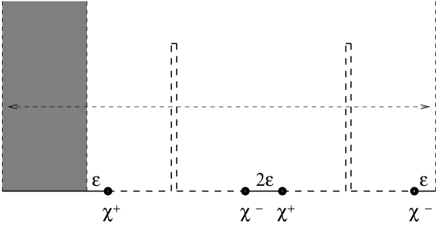
Figure 23: The geometry involved in the computation of $|{\cal B}^{\prime}_{\alpha,t}*{\cal B}^{\prime}_{\alpha,t}\rangle$. The boundary components labeled by thick continuous line represent $BCFT$ boundary conditions and the boundary components labeled by thick broken lines label $BCFT^{\prime}$ boundary conditions. The coordinate labels of various points are identical to those in Fig.20.

The computation of $|{\cal B}^{\prime}_{\alpha,t}*{\cal B}^{\prime}_{\alpha,t}\rangle$ is straightforward using the gluing rules in the $\widehat{z}$ coordinate system. The result is:

$$\langle{\cal B}_{\alpha,t}^{\prime}*{\cal B}_{\alpha,t}^{\prime}|\phi\rangle=(2\epsilon)^{4h}\Bigl{\langle}f\circ\phi(0)\chi^{+}({\pi\over 4}+\epsilon)\chi^{-}({\pi\over\alpha}-{\pi\over 4}-\epsilon)\chi^{+}({\pi\over\alpha}-{\pi\over 4}+\epsilon)\chi^{-}({2\pi\over\alpha}-{3\pi\over 4}-\epsilon)\Bigr{\rangle}_{{\cal C}^{\prime}_{\alpha,t}}\,.$$ (10.5)

The geometry of ${\cal C}^{\prime}_{\alpha,t}$ has been shown in Fig.23. This correlation function can be evaluated by mapping it to the UHP via the map given in eq.(8.10). As shown in section 8.2, as $t\to 1$ this approaches eq.(8.21), with part of the ${\cal C}^{\prime}_{\alpha,t}$ plane in the middle collapsing to a point in the $\widehat{z}$ plane. In this case this part includes the insertion $\chi^{-}(\pi/\alpha-\pi/4-\epsilon)\chi^{+}(\pi/\alpha-\pi/4+\epsilon)$, and hence this can be replaced by the leading term in the operator product expansion which is $(2\epsilon)^{-2h}$. Thus in the $t\to 1$ limit, we can rewrite (10.5) as,

$$\langle{\cal B}^{\prime}_{\alpha}*{\cal B}_{\alpha}^{\prime}|\phi\rangle=(2\epsilon)^{2h}\Bigl{\langle}f\circ\phi(0)\chi^{+}({\pi\over 4}+\epsilon)\chi^{-}(-{\pi\over 4}-\epsilon)\Bigr{\rangle}_{{\cal C}^{\prime}_{\alpha,1}}\,,$$ (10.6)

where we have used the periodicity in the $\widehat{z}$ plane to replace $\chi^{-}(2\pi/\alpha-3\pi/4-\epsilon)$ by $\chi^{-}(-\pi/4-\epsilon)$. Using the result of section 8.2 that the map $g_{\alpha}(\widehat{z})$ defined in eq.(10.3), that maps ${\cal C}_{\alpha}$ to the upper half plane, also maps ${\cal C}^{\prime}_{\alpha,t}$ to the upper half plane for $t=1$, we have:

$$\langle{\cal B}^{\prime}_{\alpha}*{\cal B}_{\alpha}^{\prime}|\phi\rangle=(2\epsilon)^{2h}\Bigl{\langle}g_{\alpha}\circ f\circ\phi(0)g_{\alpha}\circ\chi^{+}({\pi\over 4}+\epsilon)g_{\alpha}\circ\chi^{-}(-{\pi\over 4}-\epsilon)\Bigr{\rangle}_{UHP}\,.$$ (10.7)

Comparing eqs.(10.4) and (10.7) we see that

$$\langle{\cal B}^{\prime}_{\alpha}|=\langle{\cal B}^{\prime}_{\alpha}*{\cal B}^{\prime}_{\alpha}|\,,$$ (10.8)

as we wanted to show. We end this section by noting that this construction can be easily generalized to construct any of the projectors discussed in section 5 associated with a general BCFT.

11 Concluding Remarks

In this paper we have given a rather general discussion of projectors of the open string $*$-algebra and split wave-functionals. It was found that in addition to the sliver, infinitely many projectors exist which have pure geometrical interpretation as surface states. We have also seen that such surface states, in general, can be viewed as tensor products of half-string surface states. This viewpoint makes it clear that the half-string surface states are naturally defined with the same open string boundary conditions as the full string states. Moreover, all projectors are clearly recognized as being invariant under opposite constant translations of the half strings. We have illustrated in detail our general considerations, by discussing explicitly several interesting projectors.

While we have indicated that the projectors considered here are expected to be equivalent in that they define physically equivalent solutions of vacuum string field theory, our focus on specific projectors and their properties may have applications in other contexts. For example, it seems clear that OSFT solutions are not projectors. It follows, that if OSFT solutions are eventually built in terms of deformations of projectors, particular projectors could be of special use. As noted, level expansion does seem to single out the butterfly as a special projector. There may still be other surface state projectors deserving particular attention which we have not uncovered.

One question we have not attempted to investigate is how the approach of the midpoint to the boundary controls the behavior of the projector. While $f(\xi=i)=\infty$ seems necessary to have a projector, it may be of interest to understand the full significance the behavior of $f$ near $\xi=i$. We have already seen that this behavior controls the boundary conditions satisfied by the half string states.

In this paper we have only considered string fields which have a purely geometric interpretation as surface states associated to Riemann surfaces. All such string fields belong to the Virasoro module on the vacuum. We have uncovered the general geometric mechanism that gives rise to rank-one surface state projectors. It should be kept in mind that there are many projectors that lie outside the Virasoro module of the vacuum and do not have a purely geometric interpretation. For example there are squeezed states built with flat space oscillators that star-multiply to themselves but are not surface states.

It has been recently recognized [40, 43] that the open string star product can be interpreted as a continuous tensor product of mutually commuting two-dimensional Moyal products. This algebraic approach is likely to shed new light on projectors, and it will be interesting to understand in detail the connection with the geometric methods of the present paper. A complete understanding of projectors could well help eventually give a concrete description of the star-algebra. In fact, given the central role of projectors in the study of non-commutative field theory, it is natural to expect that star-algebra projectors will have an important role in our future understanding of string field theory.

Acknowledgements. We would like to thank M. Schnabl for discussions on the matters presented here. The work of L.R. was supported in part by Princeton University “Dicke Fellowship” and by NSF grant 9802484. The research of A.S. was supported in part by a grant from the Eberly College of Science of the Penn State University. The work of B.Z. was supported in part by DOE contract #DE-FC02-94ER40818.

Appendix A Numerical Computations Involving the Butterfly

In this appendix we shall present numerical results for computations involving the butterfly at various levels of approximation. We approximate the butterfly by truncating it to a given level $L$, and calculate various star products keeping only terms up to level $L$. The results are given in Tables 1, 2 and 3. The last column gives the expected answers, and the last but one column gives the extrapolation of the numerical answers to infinite level using a fit of the form $a+b/L+c/L^{2}$.

Table 1 contains numerical results for the square of the butterfly. As we see from this table, as we include more and more terms in the expression for the butterfly, the closer is its square to the expected answer.

We can also test the property (5.4) that the butterfly is a rank-one projector. We need to work in a unitary BCFT, so we choose to consider butterfly states $|{\cal B}^{c=1}\rangle$ built with Virasoro generators of central charge one. Star multiplication of surface states in this theory works as in the $c=0$ case but with extra (infinite) overall factors arising from the conformal anomaly. These infinite factors are regulated by the level truncation procedure and we ignore them, considering the results up to their overall normalization. In Table 2 and Table 3 we present the numerical results for the normalized products $|{\cal B}^{c=1}\rangle*|0\rangle*|{\cal B}^{c=1}\rangle$ and $|{\cal B}^{c=1}\rangle*L_{-2}|0\rangle*|{\cal B}^{c=1}\rangle$. From (5.4) we expect these products to be proportional to the butterfly, and indeed this is seen to hold more and more accurately as the level is increased.

These numerical results confirm the formal arguments of this paper that the butterfly is a rank-one projector of the $*$-algebra.

	$L=2$	$L=4$	$L=6$	$L=8$	$L=10$	$L=12$	$L=\infty$	$Exp$
$|0\rangle$	1.00000	1.00000	1.00000	1.00000	1.00000	1.00000	1.00000	1.00000
$L_{-2}|0\rangle$	-0.43230	-0.46035	-0.47214	-0.47858	-0.48263	-0.48540	-0.49981	-0.50000
$L_{-4}|0\rangle$	0	-0.00351	-0.00213	-0.00146	-0.00108	-0.00084	0.00021	0.00000
$L_{-2}L_{-2}|0\rangle$	0	0.10845	0.11309	0.11567	0.11732	0.11847	0.12307	0.12500
$L_{-6}|0\rangle$	0	0	0.00168	0.00117	0.00087	0.00068	0.00005	0.00000
$L_{-4}L_{-2}|0\rangle$	0	0	0.00040	0.00027	0.00021	0.00017	0.00003	0.00000
$L_{-3}L_{-3}|0\rangle$	0	0	-0.00034	-0.00023	-0.00016	-0.00012	0.00001	0.00000
$(L_{-2})^{3}|0\rangle$	0	0	-0.01771	-0.01843	-0.01887	-0.01918	-0.02017	-0.02083

Table 1: Numerical results for the coefficients of $|{\cal B}\rangle*|{\cal B}\rangle$.

	$L=2$	$L=4$	$L=6$	$L=8$	$L=10$	$L=12$	$L=\infty$	$Exp$
$|0\rangle$	1.00000	1.00000	1.00000	1.00000	1.00000	1.00000	1.00000	1.00000
$L_{-2}|0\rangle$	-0.39892	-0.44581	-0.46296	-0.47192	-0.47743	-0.48115	-0.50002	-0.50000
$L_{-4}|0\rangle$	0	-0.00617	-0.00231	-0.00136	-0.00093	-0.00069	0.00009	0.00000
$L_{-2}L_{-2}|0\rangle$	0	0.09982	0.10808	0.11217	0.11465	0.11633	0.12312	0.12500
$L_{-6}|0\rangle$	0	0	0.00349	0.00143	0.00088	0.00063	-0.00002	0.00000
$L_{-4}L{-2}|0\rangle$	0	0	0.00117	0.00054	0.00033	0.00024	-0.00005	0.00000
$L_{-3}L_{-3}|0\rangle$	0	0	-0.00005	-0.00011	-0.00009	-0.00007	0.00000	0.00000
$L_{-2}L_{-2}L_{-2}|0\rangle$	0	0	-0.01652	-0.01761	-0.01825	-0.01867	-0.02007	-0.02083

Table 2: Numerical results for the coefficients of $|{\cal B}^{c=1}\rangle*|0\rangle*|{\cal B}^{c=1}\rangle$. The coefficient of $|0\rangle$ in the result has been normalized to one.

	$L=2$	$L=4$	$L=6$	$L=8$	$L=10$	$L=12$	$L=\infty$	$Exp$
$|0\rangle$	1.00000	1.00000	1.00000	1.00000	1.00000	1.00000	1.00000	1.00000
$L_{-2}|0\rangle$	-0.48377	-0.49010	-0.48462	-0.48562	-0.48720	-0.48862	-0.48519	-0.50000
$L_{-4}|0\rangle$	0	-0.05238	-0.00861	-0.00461	-0.00312	-0.00233	-0.00689	0.00000
$L_{-2}L_{-2}|0\rangle$	0	0.11387	0.11410	0.11565	0.11712	0.11823	0.12254	0.12500
$L_{-6}|0\rangle$	0	0	0.02146	0.00456	0.00247	0.00166	0.00258	0.00000
$L_{-4}L{-2}|0\rangle$	0	0	0.00288	0.00054	0.00043	0.00035	0.00086	0.00000
$L_{-3}L_{-3}|0\rangle$	0	0	-0.00083	-0.00093	-0.00055	-0.00038	0.00059	0.00000
$L_{-2}L_{-2}L_{-2}|0\rangle$	0	0	-0.01738	-0.01795	-0.01848	-0.01886	-0.02016	-0.02083

Table 3: Numerical results for the coefficients of $|{\cal B}^{c=1}\rangle*L_{-2}|0\rangle*|{\cal B}^{c=1}\rangle$. The coefficient of $|0\rangle$ in the result has been normalized to one.

References

- [1] A. Sen, Int. J. Mod. Phys. A14, 4061 (1999) [hep-th/9902105]; hep-th/9904207; JHEP 9912, 027 (1999) [hep-th/9911116].
- [2] E. Witten, “Noncommutative Geometry And String Field Theory,” Nucl. Phys. B 268, 253 (1986).
- [3] L. Rastelli, A. Sen and B. Zwiebach, “String field theory around the tachyon vacuum”, hep-th/0012251.
- [4] D. Gaiotto, L. Rastelli, A. Sen and B. Zwiebach, “Ghost structure and closed strings in vacuum string field theory,” arXiv:hep-th/0111129.
- [5] L. Rastelli, A. Sen and B. Zwiebach, “Classical solutions in string field theory around the tachyon vacuum,” hep-th/0102112.
- [6] L. Rastelli, A. Sen and B. Zwiebach, “Half-strings, Projectors, and Multiple D-branes in Vacuum String Field Theory”, hep-th/0105058.
- [7] L. Rastelli, A. Sen and B. Zwiebach, “Boundary CFT Construction of D-branes in Vacuum String Field Theory,” hep-th/0105168.
- [8] Y. Matsuo, “BCFT and sliver state,” Phys. Lett. B 513, 195 (2001) [arXiv:hep-th/0105175].
- [9] J. R. David, “Excitations on wedge states and on the sliver,” JHEP 0107, 024 (2001) [arXiv:hep-th/0105184].
- [10] L. Rastelli, A. Sen and B. Zwiebach, “Vacuum string field theory,” hep-th/0106010.
- [11] D. J. Gross and W. Taylor, “Split string field theory. I,” JHEP 0108, 009 (2001) [arXiv:hep-th/0105059].
- [12] D. J. Gross and W. Taylor, “Split string field theory. II,” JHEP 0108, 010 (2001) [arXiv:hep-th/0106036].
- [13] K. Furuuchi and K. Okuyama, “Comma vertex and string field algebra,” JHEP 0109, 035 (2001) [arXiv:hep-th/0107101].
- [14] H. Hata and T. Kawano, “Open string states around a classical solution in vacuum string field theory,” hep-th/0108150.
- [15] I. Kishimoto, “Some properties of string field algebra,” JHEP 0112, 007 (2001) [arXiv:hep-th/0110124].
- [16] P. Mukhopadhyay, “Oscillator representation of the BCFT construction of D-branes in vacuum string field theory,” JHEP 0112, 025 (2001) [arXiv:hep-th/0110136].
- [17] N. Moeller, “Some exact results on the matter star-product in the half-string formalism,” arXiv:hep-th/0110204.
- [18] H. Hata and S. Moriyama, “Observables as Twist Anomaly in Vacuum String Field Theory,” arXiv:hep-th/0111034.
- [19] K. Okuyama, “Siegel gauge in vacuum string field theory,” arXiv:hep-th/0111087.
- [20] L. Rastelli, A. Sen and B. Zwiebach, “A note on a proposal for the tachyon state in vacuum string field theory,” hep-th/0111153.
- [21] L. Rastelli, A. Sen and B. Zwiebach, “Star algebra spectroscopy,” arXiv:hep-th/0111281.
- [22] I. Kishimoto and K. Ohmori, “CFT description of identity string field: Toward derivation of the VSFT action,” arXiv:hep-th/0112169.
- [23] R. Rashkov and K. S. Viswanathan, “A note on the tachyon state in vacuum string field theory,” arXiv:hep-th/0112202; “A proposal for the vector state in vacuum string field theory,” arXiv:hep-th/0201229.
- [24] I. Y. Arefeva, A. A. Giryavets and P. B. Medvedev, “NS matter sliver,” arXiv:hep-th/0112214.
- [25] I. Y. Arefeva, D. M. Belov and A. A. Giryavets, “Construction of the vacuum string field theory on a non-BPS brane,” arXiv:hep-th/0201197.
- [26] M. Marino and R. Schiappa, “Towards vacuum superstring field theory: The supersliver,” arXiv:hep-th/0112231.
- [27] K. Okuyama, “Ghost Kinetic Operator of Vacuum String Field Theory,” arXiv:hep-th/0201015.
- [28] L. Bonora, D. Mamone and M. Salizzoni, “B field and squeezed states in vacuum string field theory,” arXiv:hep-th/0201060.
- [29] K. Okuyama, “Ratio of tensions from vacuum string field theory,” arXiv:hep-th/0201136.
- [30] T. Okuda, “The equality of solutions in vacuum string field theory,” arXiv:hep-th/0201149.
- [31] H. Hata, S. Moriyama and S. Teraguchi, “Exact results on twist anomaly,” arXiv:hep-th/0201177.
- [32] L. Rastelli and B. Zwiebach, “Tachyon potentials, star products and universality,” JHEP 0109, 038 (2001) [arXiv:hep-th/0006240].
- [33] V. A. Kostelecky and R. Potting, “Analytical construction of a nonperturbative vacuum for the open bosonic string,” Phys. Rev. D 63, 046007 (2001) [hep-th/0008252].
- [34] G. Moore and W. Taylor, “The singular geometry of the sliver” arXiv:hep-th/0111069.
- [35] M. Schnabl, “Anomalous reparametrizations and butterfly states in string field theory” arXiv:hep-th/0202139.
- [36] A. LeClair, M. E. Peskin and C. R. Preitschopf, “String Field Theory On The Conformal Plane. 1. Kinematical Principles,” Nucl. Phys. B 317, 411 (1989); Nucl. Phys. B 317, 464 (1989).
- [37] D. J. Gross and A. Jevicki, “Operator Formulation Of Interacting String Field Theory,” Nucl. Phys. B283, 1 (1987).
- [38] I. Bars and Y. Matsuo, “Associativity Anomaly in String Field Theory,” arXiv:hep-th/0202030.
-
[39]
H. M. Chan, J. Bordes, S. T. Tsou and L. Nellen,
Phys. Rev. D 40 (1989) 2620;
J. Bordes, H. M. Chan, L. Nellen and S. T. Tsou, Nucl. Phys. B 351 (1991) 441;
J. Bordes, A. Abdurrahman and F. Anton, Phys. Rev. D 49 (1994) 2966 [arXiv:hep-th/9306029];
A. Abdurrahman, F. Anton and J. Bordes, Nucl. Phys. B 411 (1994) 693;
A. Abdurrahman and J. Bordes, Phys. Rev. D 58 (1998) 086003;
T. Kawano and K. Okuyama, “Open string fields as matrices,” JHEP 0106, 061 (2001) [arXiv:hep-th/0105129]. - [40] I. Bars, “Map of Witten’s * to Moyal’s *,” Phys. Lett. B 517, 436 (2001) [arXiv:hep-th/0106157].
- [41] I. Ellwood, B. Feng, Y. H. He and N. Moeller, “The identity string field and the tachyon vacuum,” JHEP 0107, 016 (2001) [arXiv:hep-th/0105024].
- [42] M. Schnabl, “Wedge states in string field theory,” arXiv:hep-th/0201095.
- [43] M. R. Douglas, H. Liu, G. Moore and B. Zwiebach, “Open String Star as a Continuous Moyal Product,” arXiv:hep-th/0202087.