Cosmological Creation of D-branes and anti-D-branes

Abstract:

We argue that the early universe may be described by an initial state of space-filling branes and anti-branes. At high temperature this system is stable. At low temperature tachyons appear and lead to a phase transition, dynamics, and the creation of D-branes. These branes are cosmologically produced in a generic fashion by the Kibble mechanism. From an entropic point of view, the formation of lower dimensional branes is preferred and $D3$ brane-worlds are exponentially more likely to form than higher dimensional branes. Virtually any brane configuration can be created from such phase transitions by adjusting the tachyon profile. A lower bound on the number defects produced is: one D-brane per Hubble volume.

1 Introduction

In this article we introduce the physics of brane anti-brane systems to cosmologists and their cosmology to string theorists. Recently, there has been much interest in the cosmology of branes. However, little has been written about their origin and their anti-particles (anti-branes) which are literally the flip side of branes.

Branes and anti-branes are unlike the point particles of the standard cosmology; they are inherently non-perturbative. They are solitons and are very heavy at weak coupling. If a strongly coupled phase existed during the very early universe, branes may have been perturbative objects in the coupling $1/g_{s}$. When $g_{s}\rightarrow\infty$, then $m_{Dp}\sim 1/g_{s}\rightarrow 0$ and branes become virtually massless and may have been pair produced[1]. Because of their intricate substructure (they possess a gauge theory on their world-volume), their production may have been entropically more favorable than the production of elementary particles. Large string coupling corresponds to a large eleventh dimension since, $g_{s}\sim R_{11}$, implying that a strongly coupled universe would likely be eleven dimensional and described by M-theory  [2]. A universe originating from a M-theory initial state would thus presumably be populated by large numbers of branes of different dimensionalities.

However, little is known about such a strongly coupled era and M theory. Thus, it is difficult to describe the pair production of branes and anti-branes in any concrete way. But, non-perturbative objects such as monopoles and cosmic strings are thought to have been produced in the early universe through well understood processes – as topological defects created during various phase transitions [3]. In this paper we show that branes and anti-branes may have been easily produced in a similar way – through a tachyonic phase transition, obviating the need for pair production via a Schwinger type mechanism. This so-called tachyonic phase transition is well known, and has so far been thought of as a formal mathematical device. We will elevate it to a dynamical mechanism motivated by certain ideas from topological K-theory.

A universe in which branes are produced should also contain anti-branes. A brane differs from an anti-brane only by possessing an opposite (Ramond-Ramond) charge. The charge of a D-brane corresponds to an orientation. Hence, a $\bar{D}p$ anti-brane is simply a brane flipped over (rotated by $\pi$) [4]. It is hard to understand why the early universe may have preferred a particular orientation. Thus, if branes were ubiquitous early on, it is likely that anti-branes were too. From a technical standpoint, anti-branes are also required if the early universe was compact and cosmologically unusual objects such as orientifolds were absent. Tadpole cancellation requires them [5]. (Orientifolds are unusual because they represent boundaries of the universe and lead to non-local effects.)

Phase transitions are ideal for producing topological defects. But they often lead to an embarrassment of riches: too many are produced. For example, in many GUT phase transitions enough monopoles are created to dominate the energy density of the universe and cause it to re-collapse [6]. We find that generic tachyonic phase transitions producing branes lead to similar problems: over-abundances of branes and anti-branes.

In this paper we will try to answer the following questions: (1) were D-branes produced after the big bang; (2) if so, how; (3) do they lead to a brane problem, analogous to the monopole problem causing the universe to re-collapse?

Most of our discussion refers to a universe modeled by Type IIB string theory. Generalizations to Type IIA or Type I theory are straightforward. The picture we construct of brane anti-brane cosmology is the following.

$\bullet$ The universe starts as a stack of space-filling $D9-\bar{D}9$ brane anti-brane pairs. The $D9-\bar{D}9$ pairs may either be thought of as describing the initial state of the universe, or as produced during a high temperature era when large dimensional branes were most easily created.

$\bullet$ At high temperature, $T>T_{H}/\sqrt{g_{s}N}$, the system is stable [7]. No tachyons, which are present in brane anti-brane systems at zero temperature, exist. ($T_{H}$ is the Hagedorn temperature, $N$ is the number of initial coincident $D9-\bar{D}9$ brane anti-brane pairs, and $g_{s}$ is the closed string coupling). Because of the brane tensions, and matter on the branes (gas of open string), the branes expand and the temperature decreases. As the temperature drops the potential of open strings transforming under the bi-fundamental representation of the $U(N)\times U(N)$ gauge symmetry changes.

$\bullet$ At $T\sim T_{H}/\sqrt{g_{s}N}$ the potential for those open strings develops a double well structure and the strings become tachyonic. The tachyons then condense by rolling to the bottom of their potential where the $U(N)\times U(N)$ gauge symmetry is broken to a smaller group $G$.

$\bullet$ Upon tachyon condensation, the $D9$ branes and $\bar{D}9$ branes disappear. The tachyons cause their annihilation [8]. Cosmological topological obstructions via the Kibble mechanism generically arise. Once the tachyons roll down to the minima of their potential, $D(9-2k)$ branes corresponding to non-zero homotopy groups, $\pi_{2k-1}({\cal{M}}=U(N))$ are produced as topological defects. Exotic spatial profiles for the tachyon field at the bottom of its potential, $V(t)$, may lead to exotic brane configurations, such as intersecting branes, etc. Because the universe at this stage is weakly coupled and at a lower temperature, entropy arguments favor the formation of lower dimensional defects over higher dimensional ones. In particular $D3$ braneworlds are exponentially more likely to form than higher dimensional branes. In Type IIA theory, $D(2p)$ branes are generically produced by the Kibble mechanism. Unstable non-BPS $D(2p)$ ($D(2p+1)$) branes in Type IIB (Type IIA) may also be formed for $p$ an integer. However, in the absence of any stabilization mechanisms (orientifolds, etc.), they soon decay within a few string times after their formation.

$\bullet$ The production of branes occurs cosmologically and in a generic fashion. By causality, at least one brane per Hubble volume is created. These branes lead to a brane problem and severe cosmological difficulties.

String theory is not well understood in curved spaces. Thus we have made efforts to insure that most of our results are independent of the spacetime metric and are model independent. For example, tachyon condensation is a background independent process, as the shape of tachyon potential is fixed. Only a prefactor of the potential, the brane tension, is model dependent. The formation of defects is a topological process depending on the homotopy groups of the tachyon potential. Entropy arguments based on bulk properties of branes are used to postulate that lower dimensional branes are favored as end products of tachyon condensation. Also, the number of $Dp$ branes filling spacetime – one per Hubble volume – is an argument based on topology and causality.

The plan of the paper is as follows. In section 2 we examine whether the universe, modeled by Type IIB theory, may have begun from an initial state of $D9-\bar{D}9$ brane anti-brane pairs. In section 3 we describe the properties of a $D9-\bar{D}9$ system, and more generally the properties of brane anti-brane systems. Next, in section 4 we explain how lower dimensional branes may have filled the early universe. In section 5, we quote the analogous results for Type IIA theory. Finally, in section 6 we address some possible objections to our results.

2 An Initial State of $N$ $D9-\bar{D}9$ Brane pairs

2.1 Motivation

In recent years there has been a great multitude of brane universe models. The original ADD scenario started out as a flat D-brane in Minkowski space [9]. Then came the Randall-Sundrum models: brane(s) embedded in adS [10]. Subsequently, many variations appeared, like the manyfold universe (a brane folded on top of itself), and intersecting brane models [11]. Such models, though apparently disparate, possess enough unifying characteristics to allow a study of the whole gamut of models using only a few tools. They can all be built out of pairs of $D9$ branes and $\bar{D}9$ anti-branes in Type IIB string theory, or the unstable $D9$ branes of Type IIA string theory [12, 13, 14].

Recently, the K-theory classification of D-brane charges has taught us that any D-brane configuration in type IIB string theory can be built out of $N$ $D9-\bar{D}9$ brane anti-brane pairs. On their world-volumes, the 9-branes and anti-branes possess tachyon fields and fluxes akin to electromagnetic fluxes. One starts with a collection of $D9-\bar{D}9$ branes and adjusts the tachyon fields and fluxes on the 9-branes. A phase transition then occurs turning the original constituents into the configuration of choice. D-brane configurations in Type IIA string theory can similarly be constructed from unstable $D9$ branes and their world-volume fields, although subtleties arise requiring the use of K-homology [15]. Hence, we can study any brane world scenario by studying 9-branes and the tachyons and fluxes on them.

Such 9-branes may be thought of as mathematical devices to create brane configurations. However, they can also be taken to be real. We treat them as physical objects and model the early universe as emerging from an initial state of $D9-\bar{D}9$ branes. (We pick Type IIB theory as our starting point.)

The $D9-\bar{D}9$ branes may be thought of as an initial state with the following properties. It is an open string vacuum state, since $D9-\bar{D}9$ pairs are a solution to the “equations of motion” of open strings. This vacuum is unstable at zero temperature. But, it is thought to be stable at high temperature. Since the branes are space-filling, there is no ad hoc partition of spacetime into Neumann and Dirichlet directions. Hence, apart from compactification issues, such a state describes an isotropic and homogeneous universe. Also, such an open string vacuum state necessarily contains open and closed string excitations. Closed strings correspond to gravity and open strings correspond to gauge fields like photons or gluons and one expects the early universe to have possessed gravitational and gauge degrees of freedom. Gravity appears on the space-filling branes because of worldsheet duality. This duality implies that open string theories necessarily contain closed strings. In the case of $Dp$ branes, the closed strings are in the bulk. However, for space-filling branes, there is no bulk, or rather the bulk coincides with the world-volume of the branes [16].

Previous string cosmology scenarios such as the pre-big bang proposal, have always taken the closed string vacuum state as an initial state [17]. Closed string theories do not necessarily contain open strings (gauge fields). Thus the description of the early universe as an open string vacuum seems more natural.

The rationality of an initial state of $N$ $D9-\bar{D}9$ branes can also be argued from thermodynamics. It appears entropically favorable to create large dimensional branes at very high energy densities and weak coupling [18].

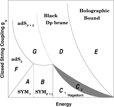
Figure 1: The phase diagram of D-branes as a function of the closed string coupling, $g_{s}$ and energy, $E$.

We recall the D-brane phase diagram discussed in Abel, Barbon, Kogan and Rabinovici  [18, 19, 20]. A D-brane admits two different thermodynamic descriptions. At weak coupling, the entropy of a brane is dominated by the gas of open (super Yang-Mills) strings on its world-volume, which corresponds to regions $A$ and $B$ in figure 1. If the temperature is raised, the increased energy density is transferred to the open strings. Since the mass of the strings is proportional to their length, the open strings grow and start to explore the surrounding space. If compact directions exist, the strings may wind these directions leading to winding modes. This corresponds to the Hagedorn regime, regions $C_{1}$ and $C_{2}$. At very high energy density the energy of a D-brane is dominated by the cloud of open strings on it. In region $C_{2}$ the energy of the gas equals, and exceeds, the rest mass of the D-brane. If the energy is raised further, the Jeans mass is exceeded and a black hole forms, region $D$.

At strong coupling D-branes have a different description. The entropy of a brane in this regime is dominated by its geometrical entropy – akin to the area of a black hole. A finite temperature $Dp$ brane has horizons. At low temperatures it has an $adS_{p+2}$ geometry, region $G$. At sufficiently low temperatures the brane can be described as a collection of “smeared” $D0$ branes whose geometry is $adS_{2}$, region $F$. At very high temperatures, the horizons of the $adS_{p+2}$ geometry shift and the $Dp$ brane turns into a black hole, region $D$. As the energy is further increased the black hole grows until it fills up the entire space and reaches the holographic bound, region $E$.

The dotted line partitioning regions $C_{1}$ and $C_{2}$ denotes when the energy $E$ of the open string gas becomes larger than the $Dp$ brane mass, $m_{Dp}\sim 1/g_{s}$. This region may be unstable to the spontaneous production of D-branes or anti-branes leading to the screening of any already existing Ramond-Ramond charge. Abel, et al.,  [18] assert that in thermal equilibrium the following reaction should be common in region $C_{2}$: $D+\bar{D}\leftrightarrow X+X$, where $X$ are massless fields. The chemical potential of the massless fields is zero implying that in equilibrium, $\mu+\bar{\mu}=0$, where $\mu$ and $\bar{\mu}$ are the chemical potentials of the branes and anti-branes respectively. In the absence of any CP violation, and for significant brane production, symmetry dictates that $\mu=\bar{\mu}=0$. Because of their considerable structure (a world-volume gauge theory), branes can be crudely modeled as particles having internal structure and obeying Boltzmann statistics. The chemical potential is then

$$\mu\sim\ln\left(\frac{V_{\perp}}{N}\sum_{\vec{p}_{\perp},n}e^{-\beta E(\vec{p}_{\perp},n)}\right)$$ (1)

The sum is over the center of mass motion of a brane and its quantum numbers $n$. The energy is $E(\vec{p}_{\perp},n)=M_{p}+\vec{p}^{2}_{\perp}/2m_{Dp}+\epsilon_{n}$. The $\epsilon_{n}$ are the internal excitations and represent open string excitations on a D-brane. The free energy of the open string gas on a $Dp$ brane is $e^{-\beta F_{g}}=\sum_{n}e^{-\beta\epsilon_{n}}$. If $\mu=0$, eq. 1 can be inverted giving,

$$\frac{V_{\perp}}{N}\sim e^{-\beta m_{Dp}}\sum_{n}e^{-\beta\epsilon_{n}}\int d\vec{p}_{\perp}e^{-\beta\vec{p}^{2}_{\perp}/2m_{Dp}}=e^{-\beta(m_{Dp}+F_{g})}\left(\frac{m_{Dp}}{\beta}\right)^{d_{\perp}/2}$$ (2)

Near the Hagedorn temperature for $p>6$, the free energy, $F_{g}$, diverges negatively. Thus unsuppressed pair production of large dimensional branes may occur in Type IIB string theory. The free energy diverges because, above $p=6$ the system is limiting. Increases in energy lead to more winding modes and an energy pile-up on the branes. Note, the density of states is proportional to the (volume of the brane)/(volume of the transverse space). For $p<6$, the system is not limiting, and can lose its energy to the closed string bath (in the bulk).

It would have been impossible to spontaneously produce heavy defects like D-branes at high temperature, had they not possessed a world-volume gauge theory. Because of their intricate structure it is entropically favorable to produce them at high temperature. We can make this more obvious by focusing on the gauge group on the branes and noting how it influences the free energy [7].

Consider a configuration of $N$ branes and $N$ anti-branes. Let $k_{1}$ and $k_{2}$ be two positive numbers less than unity. Suppose $k_{1}N$ branes are coincident. Then a $U(k_{1}N)$ gauge theory will appear increasing the entropy by a factor of $k_{1}N$. If $k_{2}N$ brane anti-brane pairs are coincident, then (tachyonic) open strings transforming in a bifundamental representation $(k_{2}N,\overline{k_{2}N})$ will arise. This will increase the entropy by a factor of $k_{2}^{2}N^{2}$.

Let $F_{Dp}$ be the free energy due to the center of mass motion of branes and anti-branes, and $F_{photon}$ be the entropy of the open string excitations on non-coincident branes and anti-branes. Suppose the number of branes which are coincident equals the number of anti-branes which are coincident and let $F_{gluon}$ be the free energy of a single pair of coincident branes. Let $F_{tachyon}$ be the free energy due to open string excitations on a coincident brane anti-brane pair. Finally let $F_{V(t)}$ be the free energy due to the potential energy of the tachyons. Then the free energy of the open string and D-brane system is

$$F=F_{V(t)}+F_{Dp}+F_{photon}+2k_{1}NF_{gluon}+k_{2}^{2}N^{2}F_{tachyon}$$ (3)

$F_{photon},F_{gluon}$, and $F_{tachyon}$ are the free energies of open string gases on the brane, and as discussed above, diverge negatively near the Hagedorn temperature for large $p$. Maximizing the entropy means minimizing the free energy, and the free energy as a function of $N$ looks like an inverted parabola. It is minimized by taking $N$ to infinity. This would seem to indicate that, at least in the canonical ensemble, where the system is connected to an infinite reservoir of energy, that configurations with large numbers of high dimension branes are probable.

2.2 Supersymmetry

A system of branes and anti-branes such as a pair of $D9-\bar{D}9$ breaks all supersymmetries  [8]. This may be disconcerting. However, from our point of view, it may actually be beneficial. Supersymmetry is valuable for solving the hierarchy problem at low energies. But it is problematic for cosmology because it is difficult to reconcile with time dependent metrics [22]. For example, in the simplest set up with no non-perturbative fluxes turned on, supersymmetry requires the existence of a timelike Killing spinor. A timelike Killing spinor roughly squares to a timelike Killing vector. Systems with timelike Killing vectors are stationary, and are cosmologically not very interesting.

Brane anti-brane systems are non-supersymmetric at high energies, but after undergoing tachyonic phase transitions can easily flow to supersymmetric configurations at lower energies. By adjusting the scale at which the transitions take place, one can adjust the energy at which the supersymmetry needed for the hierarchy problem is restored. Thus by breaking supersymmetry at high energies, time dependent vacuum solutions of the supergravity equations may be more easily generated and the hierarchy problem resolved by restoring supersymmetry at lower energies. The time dependence of the universe at late times would be a separate problem to solve. But it would be no harder than it is already.

3 Properties of $D9-\bar{D}9$ Systems

3.1 The Presence of Tachyons at Zero Temperature

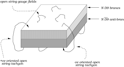
Figure 2: $N$ coincident $D9-\bar{D}9$ brane anti-brane pairs; open strings stretching between branes and anti-branes are tachyons.

Brane anti-brane systems are tachyonic at zero temperature [23]. This is because the GSO projection on the sector of open strings connecting the branes to the anti-branes is reversed [8]. Thus, instead of projecting out the tachyons in this sector, the GSO projection insures that the tachyons remain. In fact, there are two tachyons per brane and anti-brane, because strings connecting the branes to anti-branes can be oriented in two ways, see figure 2. Each pair of tachyons can be complexified into a complex tachyon field. For $N$ coincident branes and anti-branes, there are $N^{2}$ ways of connecting the $N$ branes to the $N$ anti-branes. Thus, the tachyons transform in the bifundamental representation $(N,\bar{N})$ of the gauge group on the brane: $U(N)\times U(N)$.

The existence of tachyons may be surprising as superstring theory claims to be tachyon-free. However, these tachyons are manifestations of the instability one expects from particle anti-particle attraction. The tachyon eventually leads to the annihilation of the brane and anti-brane, provided no topological obstructions to annihilation exist [8].

The tachyon field, $t$, possesses a potential $V(t)$ which depends on only $|t|$. The potential has a double well shape. Initially, the tachyon starts at the top of the potential, $t=0$, and then rolls down to the bottom, $t_{0}$. If no topological obstructions to tachyon condensation exist, then at the bottom of the well, $t=t_{0}$, the negative tachyon energy cancels the tensions of the brane and anti-brane leaving the manifestly supersymmetric closed string vacuum. Specifically, for $N$ coincident brane anti-brane pairs, as Sen [8] has argued and has been verified by  [24, 25, 26]:

$$V(t_{0})+2N\tau_{p}=0.$$ (4)

When $t=t_{0}$ the phase transition ends. Since the transition is second order, all of spacetime flows from the open string vacuum to the closed string vacuum state in a finite time. No physical open string degrees of freedom will be left and none of the false vacuum (open string vacuum) remains. The open string degrees of freedom represented by the gauge fields on the brane acquire masses and become confined. Closed string dilatonic/gravitational/RR-radiation fills the space.

A vital feature of the tachyon potential is that it can universally be written as  [27]

$$V(t)=2\tau_{p}(1+v(t)).$$ (5)

Here $v(t)$ is a dimensionless universal function of the tachyon field. It is exactly -1 at the bottom of the potential. For superstrings, the bottom is always a global minimum. Apart from the multiplicative factor, $\tau_{p}$, the tachyon potential is the same for flat D-branes, D-branes wrapped on cycles of an internal compact manifold, D-branes in the presence of a background metric or anti-symmetric tensor field. The tension, $\tau_{p}$, is the only model dependent parameter and depends on the boundary conformal/string field theory used to describe the system.

3.2 Remarks on Open String Tachyons at High Temperature

Figure 3: The tachyon potential $V(t)$ above and below the critical temperature $T_{c}$ $\sim T_{H}/\sqrt{g_{s}N}$.

The behavior of the tachyon potential at high temperature is not well understood. However, we make some remarks based on the preliminary investigation by Danielsson et al.  [7].

In field theory, it is well known that finite temperature loop corrections lead to symmetry restoration at high temperature [29]. For example a double well potential for a scalar field $\phi$ in a $\phi^{4}$ type theory will slowly change shape and become parabolic at some critical temperature. See figure 3.

The authors argue in  [7] that something similar happens to the tachyon potential. This is very significant for $D9-\bar{D}9$ physics. In a parabolic potential, the tachyon is no longer “tachyonic” and possesses a positive mass, implying that brane anti-brane systems are stable at high temperature. This insures that a universe composed of a stack of $D9-\bar{D}9$ branes is initially stable. The physical reason cited for stability is the following: by shifting the equilibrium value of the tachyon field upwards toward the symmetric point, the tachyon mass decreases. Although, it costs energy to do this, a gas of smaller mass tachyons has a larger entropy. At very high temperature, the minimum of the potential can shift to the symmetric point, $t=0$.

More concretely, the symmetric point minimizes the free energy at temperatures above a critical temperature $T_{c}$

$$T\geq T_{c}\sim\frac{T_{H}}{\sqrt{g_{s}N}}$$ (6)

where $g_{s}$ is the closed string coupling and $T_{H}$ is the Hagedorn temperature. This can be shown by considering the potential and tachyon parts of the free energy, $F_{V(t)}$ and $F_{tachyon}$ respectively. For simplicity, consider the case of a $D3-\bar{D}3$ pair, and let the tachyon potential be parameterized as in eq. (5). Then,

$$F=2\tau_{3}{\rm Tr}v(t)+\frac{\Omega_{2}}{(2\pi)^{3}}cN^{2}\beta^{-4}\int_{0}^{\infty}dxx^{2}\ln\left(\frac{1-e^{-\sqrt{x^{2}+\beta^{2}m^{2}}}}{1+e^{-\sqrt{x^{2}+\beta^{2}m^{2}}}}\right)$$ (7)

where $\tau_{3}$ is the 3-brane tension and $m$ is the mass given to the gauge bosons which gain a mass and become confined due to tachyon condensation. Here $c=8$, and is a degeneracy factor accounting for the 8 bosonic and 8 fermionic degrees of freedom. By starting at the symmetric point and letting one of the diagonal tachyons condense by an amount $\delta t$, the tachyon gains mass, the gauge bosons get a mass $\delta m$, and the free energy changes (7) by

$$\delta F=-4\tau_{3}(\delta t)^{2}+\frac{1}{2}\frac{N}{\beta^{2}}(\delta m)^{2}$$ (8)

For sufficiently large temperature, $\delta F$ is no longer negative for a tachyon rolling towards its minimum $t_{0}$. It becomes positive for $T>T_{c}$. Thus, if tachyon condensation occurs above $T_{c}$, the entropy decreases. Therefore, tachyon condensation does not occur, and the minimum of the tachyon potential can shift from $t=t_{0}$ to $t=0$.

However, this high temperature description of the open string vacuum ($t=0$) is typically non-perturbative. The Hagedorn temperature for open string systems is limiting and the temperature on the brane cannot exceed the Hagedorn temperature, $T_{H}$. Therefore, in order to satisfy eq. (6), the ’tHooft coupling $g_{s}N$ must exceed unity. Although the closed string coupling $g_{s}$ and the open string coupling $g_{s}^{1/2}$ may be small, the effective (’tHooft) coupling, $g_{s}N$, must be large. An exception to this has been suggested by Kogan.

3.3 Consequences of Topological Obstructions on Tachyon Condensation

If topological obstructions exist then the end product of tachyon condensation will not be pure vacuum; lower dimensional branes will be left over. This picture is familiar from years of work on monopoles and cosmic strings. For example, in the case of the Abelian Higgs Model, if the Higgs potential has non-zero winding such that the fundamental group is non-zero, $\pi_{1}(U(1))\neq 0$, then a cosmic string will be left after the Higgs field rolls down to a minimum of its potential [3]. Similar things happen in the tachyon case. Since the tachyon is a complex field, it can wind around a co-dimension two locus and non-zero winding around the tachyon potential leads to left over defects. The type of D-brane which is left over from tachyon condensation depends on which homotopy groups are non-zero.

A vortex, the higher dimensional analog of a cosmic string, will be left if $\pi_{1}({\cal{M}})\neq 0$, where ${\cal{M}}$ is the vacuum manifold of the tachyon potential. If the tachyons condense on $Dp$ and $\bar{D}p$ branes, then a vortex is a $D(p-2)$ brane. Similarly, if $\pi_{3}({\cal{M}})\neq 0$, then a vortex of a vortex – which is $D(p-4)$ brane will be left over. More generally, if the tachyons of a system of $D9-\bar{D}9$ branes condense, a $9-2k$ dimensional D-brane will be created if $\pi_{2k-1}({\cal{M}})\neq 0$.

The symmetry group of the vacuum manifold ${\cal{M}}$ is $U(N)$ if $N$ $D9-\bar{D}9$ branes condense. This is because, the gauge symmetry is broken to the diagonal subgroup $(U(N)\times U(N))/U(N)\sim U(N)$ once the tachyons receive expectation values. The existence of stable left over defects from tachyon condensation can be inferred from the presence of some Ramond-Ramond charge, which is measured by the K-theory group, ${{\rm K}}^{0}$. For example, ${\rm K}^{0}$ tells us that if the tachyons condense in $2k$ ($k\in{\mathbb{Z}}^{+}$) flat dimensions, such that false vacuum is left in $9-2k$ directions, that $9-2k$ D-brane charge may be left since ${\rm K}^{0}(S^{2k})={\mathbb{Z}}$. Here, $S^{2k}$ is the one point compactification of ${\mathbb{R}}^{2k}$. Now, ${{\rm K}}^{0}$ can be directly related to the vacuum manifold $U(N)$ through the homotopy groups $\pi_{2k-1}(U(N))$ and used to tell us when tachyon condensation onto ${\cal{M}}=U(N)$ will leave $Dp$ brane charge. Specifically [28],

$${{\rm K}}^{0}(S^{2k+r})=\left\{\begin{array}[]{cll}{\mathbb{Z}}&{\rm if}&r=0\\ 0&{\rm if}&r=1\end{array}\right\}=\pi_{2k-1+r}(U(N))\ \ \ \ \forall N\geq k+r,~{}k\in{\mathbb{Z}}^{+}.\$$ (9)

This means that if the tachyon field condenses in even dimensions ($r=0$) that stable $9-2k$ branes may form if $N\geq k$, and that if the tachyon condenses in odd dimensions ($r=1$) that no stable branes will form as long as $N\geq k+1$. In fact no stable defects will form for any $N$, if the tachyon condenses in odd dimensions. The homotopy groups $\pi_{2k}(U(N))$ will not generally be trivial for $N<k+1$. For example [31], if $N=k-1$ and $k\in 2{\mathbb{Z}}$, then $\pi_{2k}(U(N=k-1))={\mathbb{Z}}_{(2k!)/2}$. However, such a $9-(2k+1)$-brane described by $\pi_{2k}$, does not possess any Ramond-Ramond charge, as can be verified from the Chern-Simons part of the action. It will decay to vacuum in much the same way that the global strings of cosmic string theory, which appear due to a non-trivial $\pi_{0}$, decay via the emission of radiation. Likewise, if $N<k$ and the tachyon condenses in even dimensions, no physical/stable $D(9-2k)$ branes can form. (A lower dimensional $D(9-2k^{\prime})$ brane can of course form, for $N\geq k^{\prime}$.) Thus by restricting to the stable range $N\geq k+r$, we obtain all the physically possible/stable D-branes. Table 1 makes (9) more explicit. This is a hint of the power of K-theory. It identifies all of the possible decay products almost for free, whereas homotopy theory mistakes some unstable/unphysical configurations as stable.

$Dp$-brane	$D8$	$D7$	$D6$	$D5$	$D4$	$D3$	$D2$	$D1$	$D0$	$D(-1)$
Transverse Space	$S^{1}$	$S^{2}$	$S^{3}$	$S^{4}$	$S^{5}$	$S^{6}$	$S^{7}$	$S^{8}$	$S^{9}$	$S^{10}$
Homotopy Group	$\pi_{0}$	$\pi_{1}$	$\pi_{2}$	$\pi_{3}$	$\pi_{4}$	$\pi_{5}$	$\pi_{6}$	$\pi_{7}$	$\pi_{8}$	$\pi_{9}$
$K^{0}(S^{n})=\pi_{n-1}(U(N))$	0	${\mathbb{Z}}$	0	${\mathbb{Z}}$	0	${\mathbb{Z}}$	0	${\mathbb{Z}}$	0	${\mathbb{Z}}$
Minimum $N$	1	1	2	2	3	3	4	4	5	5

Table 1: Type IIB D brane spectrum; the second line is the 1-point compactified transverse space; minimum $N$ is the minimum number of $D9-\bar{D}9$ pairs needed to create a $Dp$ brane and is the beginning of the stable range.

At the beginning of section 2.1 we advertised brane anti-brane systems as a way of creating any brane-world model by adjusting fields on the brane anti-brane system’s worldvolume. Those fields are the fluxes and the tachyons on a $Dp-\bar{D}p$ system. Their values determine whether the homotopy groups $\pi_{2k-1}({\cal{M}})\neq 0$ and which branes form at the end of tachyon condensation. The field strength, $F$, in some sense provides the energy for the defects to form. The flux, and its generalizations are quantized. Each quanta corresponds to a single brane. For example, if $\int F$ over a 2 surface is unity, then $\pi_{1}({\cal{M}})=1$ and a $D(p-2)$ brane results. The tachyon can be thought of as determining the shape of the final brane configuration. Regions where the tachyon field is stuck at $t=0$ (the false vacuum) become part of the daughter brane. Regions where the tachyon has condensed to $t=t_{0}$ become the bulk and no brane exists there. For example, if the tachyon vanishes on a co-dimension two surface and has the value $t=t_{0}$ in the two transverse directions, a vortex will form. Generally, to produce a certain configuration such as a $D3$ intersecting a $D5$, the tachyon field must be forced to be zero on the configuration and have the value $t_{0}$ in the transverse space. One can metaphorically describe the field strength as providing the “paper” out of which to create the desired brane, and the tachyon as the scissors which allow one to cut out the desired shape.

We can demonstrate this with the following example  [8]: the construction of a $D1$ brane as a vortex on a $D3-\bar{D}3$ pair. An effective Lagrangian for the tachyon on a $D3-\bar{D}3$ can be written as ${\cal{L}}=(D_{\mu}t)^{2}-V(t)$, where the gauge covariant derivative is $D_{\mu}=\partial_{\mu}-i(A_{\mu}-A^{\prime}_{\mu})$. Here $A_{\mu}$ is the gauge field on the brane and $A^{\prime}_{\mu}$ is the gauge field on the anti-brane. A finite energy vortex will be realized if at large $r$ the tachyon takes the value $t=t_{0}$ such that $V(t)\rightarrow V(t_{0})$, and the kinetic energy vanishes: $(D_{\mu}t)^{2}\rightarrow 0$. The kinetic energy at large $r$ can be seen to vanish if there is a net quantized magnetic flux on the $D3-\bar{D}3$,

$$\frac{1}{2\pi}\int(F-F^{\prime})d^{3}x=1.$$ (10)

Eq. 10 is the tachyon field’s winding number. It is also the first Chern class of the gauge field configuration. If $A_{\mu}$ has cylindrical symmetry then eq. (10) implies that in the radial gauge $A_{r}=A^{\prime}_{r}=0$ for large $r$

$$\oint_{{\rm large}\,\,S^{1}}(A_{\theta}-A^{\prime}_{\theta})d\theta=2\pi\;\;\;\Rightarrow\;\;\;A_{\theta}-A^{\prime}_{\theta},\rightarrow 1$$ (11)

Eq.(11) and the fact that the tachyon takes values on the vacuum manifold, $t\rightarrow t_{0}e^{i\theta}$, imply that $(Dt)^{2}\rightarrow 0$, and that a vortex solution exists. Using the Chern-Simons part of the action of the $D3-\bar{D}3$ pair, one can show that the vortex has Ramond-Ramond charge and is a $D1$ brane [32]. Note, this construction is virtually the same as the cosmic string solution of the Abelian Higgs model.

If one is interested in only counting the number of daughter branes arising from tachyon condensation, one can map the K-theory group classifying the D-brane charges into cohomology, and use the total Chern class to find explicit expressions for embedded charges on a $Dp-\bar{D}p$ brane configuration. The total Chern class can be decomposed into Chern classes, $c_{i}$, whose integrals measure the fluxes and their generalizations on a brane anti-brane system. For example, the Chern classes of the system are defined as

$$c_{1} = \frac{1}{2\pi i}{\rm Tr}(F-F^{\prime})$$

$$c_{2} = \frac{1}{(2\pi i)^{2}}\left({\rm Tr}(F\wedge F-F^{\prime}\wedge F^{\prime})-({\rm Tr}F\wedge{\rm Tr}F-{\rm Tr}F^{\prime}\wedge{\rm Tr}F^{\prime})\right)$$

$$c_{3} = \cdots$$ (12)

The generalized fluxes, $\int c_{i}$, are quantized and thus measure the embedded D-brane charges in a $Dp-\bar{D}p$ system – meaning the number of branes left after tachyon condensation [13, 33]. For example, $\int c_{1}$ measures the number of $p-2$ branes minus the number of $p-2$ anti-branes, or rather the total $p-2$ brane charge left after tachyon condensation; $\int c_{2}$ measures the total $p-4$ brane charge of the system; $\int c_{3}$ measures the total $p-6$ brane charge, etc.

4 Brane Production in the Early Universe

We have learned that lower dimensional branes result from tachyon condensation when magnetic fluxes are turned on. The central result of this paper is that the fluxes needed for brane formation can be generated dynamically in an expanding universe by the Kibble mechanism. This is the same mechanism which generates defects such as cosmic strings, textures and monopoles from GUT phase transitions. These defects also require fluxes to be turned on and the Kibble mechanism provides them through cosmological dynamics.

At high temperature, $T>T_{c}$, the tachyon potential will be parabolic and a system of $N$ $D9-\bar{D}9$ branes will be stable against decay. The energy density in the brane tensions $2N\tau_{9}$, the matter density on the brane due to gauge fields, and massive modes, will act as a source for the expansion of the $D9-\bar{D}9$ branes. If the expansion is adiabatic, the temperature will decrease monotonically.

Figure 4: 8D domain wall in ${\mathbb{R}}^{10}$. The loop $C$ does not wind the vacuum manifold since $\Delta\theta\neq 2\pi$ around the loop.

When the temperature approaches $T_{c}$, tachyonic instabilities will arise as the tachyon potential takes on a double well shape. After the tachyon rolls down to the vacuum manifold ${\cal{M}}$, it will be characterized by a set of phase angles, $\{\theta_{i}\}$, and a modulus $|t_{0}|$. For example, if ${\cal{M}}=S^{1}$, then the tachyon will take the expectation value $\langle t\rangle=|t_{0}|e^{i\theta}$. However, near the temperature $T_{c}$, the tachyon field will fluctuate randomly, rolling down the potential and then rolling up via thermal fluctuations. Hence $t$ will not take on any definite values and the phase angles will fluctuate. Once the temperature falls below $T_{c}$ and reaches the Ginzburg temperature $T_{G}$, thermal fluctuations will no longer be able to push the tachyon up the potential again. At this point, once the tachyon rolls to the bottom of $V(t)$, its phase will be frozen in. Note, the Ginzburg temperature is close to $T_{c}$ and can be written as $h(g_{s})T_{c}$, where $h(g_{s})$ depends only on the string coupling and is typically close to unity [3].

In a second order phase transition such as the tachyonic transition, the correlation length of the field approaches infinity. However, expanding universes have causal horizons, which bound the distance over which causal processes can occur. In a universe with a Hubble parameter $H\sim 1/t$, causal processes can occur only within a sphere of diameter $H^{-1}$. Thus an expanding universe will have regions which are causally disconnected from each other.

Suppose that no topological obstructions in the usual sense appear such that all $N$ $D9-\bar{D}9$ pairs condense completely to vacuum. Then the tachyon field will have a magnitude $|t_{0}|$ everywhere. However, because Hubble volumes are causally disconnected and since the tachyon’s phase on ${\cal{M}}$ is randomly determined, the tachyon’s phase will generally be different in different Hubble volumes. Spacetime will thus possess a domain type structure, with the expectation value $\langle t\rangle$ varying from Hubble region to region in a relatively random way. The question answered by Kibble about cosmological phase transitions (like our tachyonic transition) was whether any residue of false vacuum remains anywhere. In particular can false vacuum be trapped at the intersection points of Hubble regions like flux tubes are trapped in a superconductor [34]?

Figure 5: Three Hubble volume sized regions $A,B,C$, intersect at a point $P$, which is actually a 7D edge. The tachyon field takes the values $t_{A},t_{B},t_{C}$ on $A,B$ and $C$ respectively. The tachyon field maps the upper loop in spacetime, $D$, which encloses $P$ to the lower loop on the vacuum manifold, $E$, and is an element of $\pi_{1}({\cal{M}})$.

The answer depends on the shapes of the Hubble regions and how they intersect. Each region is nine-dimensional. When two regions meet as in figure 4, their common boundary is 8D. There is a jump of phase angles across the boundary. However, the change in phase angle(s) around the closed curve $C$ is not a non-zero multiple of $2\pi$. Thus no winding of the potential occurs. However, if three cells meet along an edge as in figure 5, where the edge is seven dimensional and coming out of the paper, then the phase change around the closed curve $D$ enclosing the edge at $P$ will be $2\pi$. The tachyon maps $D$ onto the locus $E$ winding ${\cal{M}}$. Attempts to shrink the curve in spacetime will cause the path $E$ to move off of ${\cal{M}}$ and upwards to the false vacuum $t=0$. Thus along the edge, which is the intersection of the cells, a line defect of false vacuum will be trapped. This line defect is actually seven dimensional and corresponds to a $D7$ brane. The tachyon mapping the spacetime circle, $D$, to the circle on ${\cal{M}}$ is an element of $\pi_{1}({\cal{M}})={\mathbb{Z}}$. The non-triviality of $\pi_{1}({\cal{M}})$ can be interpreted to mean that there exists a configuration, notably the 3 intersecting cells, for which a $S^{1}$ in spacetime can be mapped to a locus winding the vacuum manifold. The winding insures that some false vacuum exists, because to conserve winding number as the spacetime circle is shrunk to zero size the tachyon must move off of ${\cal{M}}$ to the top of $V(t)$ where $t=0$. Three cells were needed because three points are needed to uniquely to determine a $S^{1}$.

Likewise, the non-triviality of $\pi_{3}({\cal{M}})$ can be interpreted to mean that there exists a configuration, notably five intersecting cells, for which a $S^{3}$ in spacetime can be mapped to a locus winding the vacuum manifold. Five cells are needed because five points uniquely determine a $S^{3}$. (Think of the $S^{3}$ as passing through the centers of five 4D balls, each of which represents a Hubble volume with a different $\langle t\rangle$.) The intersection of the cells is a 5D subspace. Winding then corresponds to the presence of a $D5$ brane at the intersection point.

In general a sphere $S^{k}$ is determined by $k+2$ points If each point corresponds to a different vacuum expectation value $\langle t_{i}\rangle$, then $\pi_{k}(U(N))={\mathbb{Z}}$ corresponds to $k+2$ cells intersecting in a $9-(k+1)$ subspace with a $D(9-(k+1))$ or $\bar{D}(9-(k+1))$ brane trapped at the intersection. See Table 2.

$Dp$-brane	$D7$	$D6$	$D5$	$D4$	$D3$	$D2$	$D1$	$D0$
Loop in ${\mathbb{R}}^{10}$	$S^{1}$	$S^{2}$	$S^{3}$	$S^{4}$	$S^{5}$	$S^{6}$	$S^{7}$	$S^{8}$
No. regions	3	4	5	6	7	8	9	10
Type IIB charge	${\mathbb{Z}}$	0	${\mathbb{Z}}$	0	${\mathbb{Z}}$	0	${\mathbb{Z}}$	0

Table 2: The number of Hubble regions with a common intersection needed to produce a $Dp$ brane; the last line gives the possible Type IIB $D$-brane charge at such an intersection.

Thus because $\pi_{7}(U(N))=\pi_{5}(U(N))=\pi_{3}(U(N))=\pi_{1}(U(N))={\mathbb{Z}}$ for sufficient $N$, tachyon condensation on a group of $D9-\bar{D}9$ pairs will generically create either $D7$ or $D5$ or $D3$ or $D1$ branes at the intersections of different Hubble regions. The specific $D$-brane which forms will depend on the dynamics of the Hubble regions and how they intersect. Table 2 shows that lower dimensional branes require more regions to have a common intersection. Although the regions are irregularly shaped, it is hard to force many regions to have a common boundary. From this point of view, it would seem that higher dimensional branes are more likely to be created. However, as we show later, energetics and entropy arguments favor lower dimensional defects.

It is interesting that the spectrum of string theory defects which cosmology creates via the Kibble mechanism is much richer than in GUTs. In order to form different defects like monopoles and cosmic strings in GUTs, one needs a complicated multi-step symmetry breaking mechanism. In our case, different defects appear because the spacetime has more dimensions; thus more homotopy groups are relevant. The $\pi_{2k-1}$ can be made non-trivial simply by increasing $N$ which enlarges the unbroken gauge group $U(N)\times U(N)$ and the broken symmetry group $U(N)$.

Since we can roughly associate one intersection to each Hubble volume, a lower bound on the number of branes formed by tachyon condensation in an expanding universe is: one brane per Hubble volume.

Below, we point out another mechanism by which the Kibble mechanism can operate which may be more realistic. However, it is based on time-dependent aspects of tachyon condensation which are not well understood.

The tachyon field is actually a matrix and consists of $N^{2}$ individual tachyon fields $t_{ij}$ where $0\leq i,j\leq N$. It is charged by the $U(N)$ gauge fields on the branes and the $U(N)$ gauge fields on the anti-branes. Thus, it transforms under the bifundamental representation of $U(N)\times U(N)$, which is broken to $U(N)$ when the tachyon field receives an expectation value on the vacuum manifold ${\cal{M}}$. Using the gauge symmetry, one can diagonalize the tachyon $t$, at every point in its evolution, and isolate the degrees of freedom in $N$ diagonal tachyon fields $t_{ii}$ which we call $t_{i}$. We label time by $\tau$. The $t_{i}$ are independent of one another. However, in the diagonal basis their classical equations of motion in flat space are the same: $\Box t_{i}=-V^{\prime}(t_{i})$, and the initial conditions are also the same $t(\tau=0)=0$. Thus classically at each point in time, the fields $t_{i}$ should be the same, $t_{1}(\tau)=t_{2}(\tau)=\cdots=t_{N}(\tau)$. However, at the temperature $T_{c}$, the fields will feel thermal fluctuations, as well as quantum perturbations of magnitude $\Delta t_{i}=H/(2\pi)$. Hence, as the tachyons roll up and down the potentials $V(t_{i})$ they will lose coherence and generally $t_{1}(\tau)\neq t_{2}(\tau)\neq\cdots\neq t_{N}(\tau)$, since the evolution of the tachyon field will be partially stochastic

$$dt_{i}=t_{i}(\tau)\mu(\tau)d\tau+t_{i}(\tau)\sigma^{2}(\tau)dW_{i}.$$ (13)

The first term in (13) is the deterministic component of $t_{i}$’s evolution. The second piece is a Brownian motion.

The lack of coherence of the $t_{i}$ will not break the gauge symmetry of $t$. However, the lack of coherence means that as the Ginzburg temperature is approached the final values of the $t_{i}$ will be frozen in at different times. This effectively means that the $N$ $D9-\bar{D}9$ brane anti-brane pairs annihilate at different times. For example, suppose $t_{3},\ldots,t_{N}$ undergo their final condensation at the same time, and suppose that $t_{1}=t_{2}$ and that $t_{1}$ and $t_{2}$ have their final values frozen in several string times after $t_{3},\ldots,t_{N}$. Hence, while $t_{1}$ and $t_{2}$ are still oscillating, the other tachyons will have disappeared and the brane anti-brane pairs and the gauge fields on their worldvolume will have as well. Thus, $t_{1},t_{2}$ will no longer see the gauge fields on the $N-2$ branes which have condensed (because the gauge fields will have become confined.) They will only see the gauge fields on the first and second brane pair and will only feel a $U(2)$ gauge symmetry. Hence the gauge symmetry on ${\cal{M}}$ will have been broken to $U(N)\rightarrow U(N-2)\times U(2)$. The last two branes can lead to brane production via the Kibble mechanism. In particular they can create 7-branes or 5-branes, since $U(2)$ is in the stable range of only $\pi_{1}$ and $\pi_{3}$. The first $N-2$ pairs may typically produce lower dimensional branes, since $U(N-2)$ is in the stable range of all the relevant homotopy groups, $\pi_{1},\pi_{3},\pi_{5},\pi_{7},\pi_{9}$ if $N$ is large.

More generally, a group of $N$ tachyons will not all condense at the same time because of perturbations and because the phases are not frozen in exactly at $T_{G}$, but in a narrow band around $T_{G}$. If the condensation is staggered such that $n_{1}$ tachyons first condense at roughly the same time, and $n_{2}$ condense a few strings times later, and so on until the last group of $n_{q}$ tachyons condense, then the gauge symmetry on ${\cal{M}}$ will be broken to $U(N)\rightarrow U(n_{1})\times U(n_{2})\times\cdots\times U(n_{q})$. The number of possible ways to condense is equal to the number of subsets of $N$ brane pairs, or rather the power set of $N$, which is $2^{N}$. This is an enormous number, and it is statistically likely that many groups $n_{j}\sim{\cal{O}}(1)$ will exist. Such $n_{i}$ can only lead to the production of high dimensional branes since $U(n_{i})$ is in the stable range of only the lower homotopy groups. If $n_{j}\gg 1$, then very low dimensional branes may result from tachyon condensation and the Kibble mechanism, as $U(n_{j}\gg 1)$ is in the stable range of all the relevant homotopy groups. This multi-step symmetry breaking is a generalization of elaborate multi-step symmetry breaking patterns in GUTs which form multiple defects like monopoles and cosmic strings.

The $q$ partitions of $n_{i},0\leq i\leq q$, imply that a lower bound on the number of branes which form is: $q$ $D$-branes per Hubble volume. These branes will typically intersect since they are extended objects, and a network of branes analogous to a string network will fill spacetime.

To determine whether the underlying physics prefers the creation of large dimensional branes ($n_{i}\gg 1$) or small dimensional branes ($n_{i}\sim 1$), we employ some crude arguments based on energetics and entropy maximization. From the point of view of energetics, one would expect the tachyons to condense in as many dimensions as possible unless the tachyon profile was set by hand. Regions where the tachyons have not condensed are filled with the false vacuum $t=0$, and possess a higher energy $V(0)$, than regions where the tachyons have condensed – regions where $V=V(t_{0})$. From a different perspective, regions which are filled with D-branes have a sizable vacuum energy since D-branes are heavy at weak string coupling. Alternatively, from an entropy point of view one might expect the large possible entropy of the gauge theory on the branes to make it entropically favorable to have large regions of false vacuum.

Consider an initial state $i$ of $N$ $D9-\bar{D}9$ pairs filling a compact toroidal spacetime. Let the toroid be square and have a radius of $r_{0}$. We would like to calculate the probability for the state $i$ to decay into a final state $f_{p}$ relative to the probability for $i$ to decay into a different state $f_{p^{\prime}}$. We will take the state $f_{p}$ to consist of a gas of $Dp$ branes wrapping $p$ cycles of the torus and a gas of gravitons in the transverse space. The state $f_{p^{\prime}}$ is similar except $Dp^{\prime}$ branes wrap $p^{\prime}$ cycles and gravitons fill the remaining transverse space. For simplicity, we will assume that the final state branes are not coincident and that no coincident brane anti-brane pairs are left.

The probability of a state, $i$, is proportional to the Euclidean partition function

$$P(i)\sim Z(i)\sim e^{-F(i)}=e^{-(U(i)-TS(i))}$$ (14)

where $F(i)$, $U(i)$ and $S(i)$ are the free energy, energy and entropy of the state $i$ respectively.

The relative probability for the decay process $i\rightarrow f_{p}$ is then

$${\cal{P}}(i\rightarrow f_{p})\equiv\frac{P(f_{p})}{P(i)}\sim\frac{e^{-F(f_{p})}}{e^{-F(i)}}\sim e^{T(S(f_{p})-S(i))}$$ (15)

The entropy of the initial state, $S(i)$, is the sum of the entropy of the tachyon and gauge field gas on the world volume of the $D9-\bar{D}9$ branes which is denoted $S_{t+g}$, and the entropy of any embedded solitonic configurations, $S_{soliton}$. Thus

$$S(i)=S_{t+g}+S_{soliton}$$ (16)

The relative probability for the two processes ${\cal{P}}(i\rightarrow f_{p})$ and ${\cal{P}}(i\rightarrow f_{p}^{\prime})$ is then, using Eq. 15,

$$\frac{{\cal{P}}(i\rightarrow f_{p})}{{\cal{P}}(i\rightarrow f_{p^{\prime}})}\equiv\frac{P(f_{p})/P(i)}{P(f_{p^{\prime}})/P(i)}\sim\frac{e^{-F(f_{p})}}{e^{-F(f_{p^{\prime}})}}\sim e^{T(S(f_{p})-S(f_{p^{\prime}}))}$$ (17)

Unsurprisingly, the relative probability depends only on the difference in entropies of the states $f_{p}$ and $f_{p^{\prime}}$. The entropy $S(f_{p})$ is a sum of the entropy of the photon gas on the $Dp$ branes $S_{\gamma}$, the entropy due to the motion of a $Dp$ brane $S_{Dp}$, and the entropy of the graviton gas in the transverse space $S_{g}$.

$$S(f_{p})=S_{\gamma}+S_{Dp}+S_{g}$$ (18)

We will ignore $S_{Dp}$ because it is negligible compared to the entropies of the relativistic graviton and photon gases, $S_{g}$ and $S_{\gamma}$.

The equation of state for a gas in $d$ spatial dimensions is $p_{ress}=\rho/d$. Here $p_{ress}$ is the pressure, and $\rho$ is the energy density. The gravitons in Eq. 18 move in $9$ spatial dimensions and the photons move in $p$ spatial dimensions. Thus,  [6],

$$S_{g} = \frac{(p_{ress}+\rho_{g})}{T}V_{g}=\frac{10}{9}\frac{\rho_{g}V_{g}}{T}=\frac{10}{9}\frac{E_{g}}{T}$$

$$S_{\gamma} = \frac{(p_{ress}+\rho_{\gamma})}{T}V_{p}=\frac{p+1}{p}\frac{\rho_{\gamma}V_{p}}{T}=\frac{p+1}{p}\frac{E_{\gamma}}{T}$$ (19)

where $T$ is the temperature, $V_{p}$ is the volume of a $p$ dimensional torus, and $\rho_{g},\rho_{\gamma}$ are the energy densities of the graviton and photon gases. $E_{g}$ and $E_{\gamma}$ are the energies of the graviton and photon gases. The volume $V_{g}$ is the nine-dimensional volume $V_{9}$ minus the volume of the daughter brane $V_{p}$.

$$V_{g}=V_{9}-V_{p}$$ (20)

Energy conservation requires

$$E=E_{g}+E_{\gamma}+E_{Dp}$$ (21)

where $E_{Dp}=\tau_{p}V_{p}$. The entropy $S(f_{p})$ is then

$$TS(f_{p})=\frac{10}{9}E_{g}+\frac{p+1}{p}E_{\gamma}=\frac{10}{9}E+\left(\frac{1}{p}-\frac{1}{9}\right)E_{\gamma}-\frac{10}{9}E_{Dp}$$ (22)

To calculate the relative probability of obtaining state $f_{p}$ or $f_{p^{\prime}}$ in Eq. 17, we can calculate $\partial S(f_{p})/\partial p$ instead of the difference, $S(f_{p})-S(f_{p^{\prime}})$.

$$\frac{\partial TS(f_{p})}{\partial p}=\left[\left(\frac{1}{p}-\frac{1}{9}\right)\rho_{\gamma}-\frac{10}{9}\tau_{p}\right]\frac{\partial V_{p}}{\partial p}<0\ \ \ \ {\rm for}\ \rho_{\gamma}(T)\ll\tau_{p}$$ (23)

If $\tau_{p}>\rho_{\gamma}(T)$ then the inequality (23) is true. This will happen if the brane is not highly excited when produced. Also, if the temperature at which the brane is produced is lower than the string scale then the inquality is valid. This may occur if cosmological expansion on the branes redshifts the energy density on the parent branes and anti-branes during tachyon condensation. Equation (23) implies that the entropy increases as the dimension of the daughter $Dp$ branes decreases. This is not surprising. One expects it to be entropically favorable to produce a gas of gravitons rather than a heavy D-brane and its world-volume photon gas. The tension of the daughter D-brane soaks up most of the energy leaving little to excite the photon gas on it. If the energy of the photon gas exceeds the energy of the brane tension, then a thick halo of open strings covers the brane and the equality in (23) is reversed. This is understandable as this is the regime in which the argument in section 2.1 favoring the production of high dimensional branes applies.

Thus, for realistic conditions entropy arguments favor the production of lower dimensional branes over the production of higher dimensional branes. This contrasts with our earlier argument that low dimension branes are more difficult to create via the Kibble mechanism. We believe, that entropy arguments are likely to prevail, although this must be explicitly checked.

¿From eq. (17) one can argue that lower dimensional branes are exponentially more likely than higher dimensional ones. ¿From a brane-world point of view this may be very attractive, as it implies that the production of branes with $p>3$ is exponentially suppressed relative to the production of $D3$ brane-worlds. This also implies that few $D3$ branes will be produced, and that mostly $D1$ branes and perhaps $D(-1)$ branes (which are instantons) will form. However, if $N$ is large the probability for the formation of a $D3$ brane becomes non-negligible and is given by a Poisson-like process.

D-strings may form on the $D3$ branes as embedded defects when a $D1$ and a $D3$, formed from two partitions, overlap. Such configurations are well known [35, 36, 37, 38]. The embedded D-strings may cause cosmological problems and may induce gravitational collapse of the brane universes. Monopoles were similar disasters for pre-inflation cosmology. Inflation at high energies is needed to dilute the $D1$ branes.[39, 40]

We now relax the condition that no topological obstructions to tachyon condensation other than the Kibble mechanism appear. In the very early universe, the open strings on the space-filling branes and anti-branes are expected to be highly excited. The $D9-\bar{D}9$ branes will be covered with a cloud of excited perturbative and non-perturbative phenomena. The excitations on the branes and anti-branes will be broadly similar. However, large fluctuations may occur, and typically, the fluxes and non-perturbative excitations will be somewhat different on the the branes and anti-branes. This is consistent, for example, with a primordial magnetic field possibly generated some time before the era of structure formation. The Chern classes, $c_{m}$ measure how the excitations differ on the branes and anti-branes. Unless the gauge field configurations on the branes and anti-branes are topologically identical, the Chern classes will be non-zero. Hence, $N$ $D9-\bar{D}9$ branes near the big bang will generally possess embedded charges.

Represent the spacetime $M$ as a product manifold $M=X\times Y$, where $Y$ is some compact submanifold. Now

$$M=\sum_{\{x~{}\in X\}}X\times Y_{x}$$ (24)

where the sum is over all points $x$ in $X$. We think of $X$ as fibered at every point $x$ by $Y$, where $Y_{x}$ is the fiber at $x$. If $c_{m}$ integrated over $Y_{x}$ is non-zero, then after tachyon condensation a $D(9-2m)$ brane will be left wrapping $Y$ at the position $x$ on $X$. Thus one $D(9-2m)$ brane will exist in one Hubble volume surrounding $x$. Unlike in the Kibble mechanism, there is a brane in only one Hubble volume. It is likely that $c_{m}$ integrated over $Y_{x}$, for many points $x$, will be non-zero. However, the number of defects created in this way – which relies on random random cosmological excitations to impose $\int_{Y_{x}}c_{m}\neq 0$ – can never compare to the number of defects created by the Kibble mechanism. However, if one so desires, one can turn on various fluxes and carefully set the tachyon field, such that when the universe exits from the tachyonic phase transition, the configuration of choice (a susy intersecting brane configuration, etc.) will exist in at least one place in the universe.

5 Type IIA Theory

All of our Type IIB results have analogs in Type IIA theory. Instead of starting with $N$ $D9-\bar{D}9$ brane anti-brane pairs as an initial state, one starts with $2N$ non-BPS $D9$ branes (or $\bar{D}9$ branes) in Type IIA theory. These branes are stable at high temperature and become tachyonic at low temperature. The tachyon potential has a double well structure, and if $2N$ $\bar{D}9$ branes are initially coincident, they will possess a $U(2N)$ gauge symmetry, which is broken on the vacuum manifold to

$${\cal{M}}_{IIA}\sim\frac{U(2N)}{U(N)\times U(N)}$$ (25)

because on ${\cal{M}}$ the tachyon field possesses $N$ identical eigenvalues $t_{0}$ and $N$ identical eigenvalues $-t_{0}$.

Topological obstructions to tachyon condensation may exist in the form of lower dimensional brane charges. However, the brane charges are measured by the K-theory group ${\rm K}^{1}$, instead of ${\rm K}^{0}$ as in Type IIB theory. ${\rm K}^{1}$ maps to the homotopy groups

$${\rm K}^{1}(S^{2k+1+r})=\left\{\begin{array}[]{cll}{\mathbb{Z}}&{\rm if}&r=0\\ 0&{\rm if}&r=1\end{array}\right\}=\pi_{2k+r}\left(\frac{U(2N)}{U(N)\times U(N)}\right)\ \ \ \ \forall N>2k+1+r,~{}k\in{\mathbb{Z}}^{+}.\$$ (26)

This time if the tachyon condenses in odd dimensions ($r=0$), stable $8-2k$ branes may form if $N\geq 2k+1$. If the tachyon condenses in even dimensions ($r=1$), no stable branes will form. As before the the stable range, $N>2k+1+r$, selects the physical states.

The K group can be mapped into cohomology, and the total Chern class can be decomposed into Chern classes, each of whose integrals measure the embedded $D$-brane charges. For example, $\int c_{1}$ measures the net $D8$ brane charge, etc.

However, in reality ${\rm K}^{1}$ doesn’t always accurately measure Type IIA brane charge. For more general spacetimes, the stable range for ${\rm K}^{1}$ begins at $N=\infty$, and thus an infinite number of branes are required to create lower dimensional defects [41]. It turns out that the K-homology group ${\rm K}_{1}$ measures Type IIA D-brane charge for finite $N$ and general spacetimes. ${\rm K}_{1}$ is dual to ${\rm K}^{1}$ in the same way that homology is Poincare dual to cohomology. By substituting ${\rm K}_{1}$ for ${\rm K}^{1}$, we find a stable range beginning at finite $N$, and everything is thought to work out [15].

The cosmological dynamics in Type IIA are similar to the dynamics in Type IIB. The matter on the $\bar{D}9$ branes causes adiabatic expansion, the temperature drops, and then tachyons appear. The tachyons condense completely to vacuum everywhere, unless embedded charges exist.

Even if no embedded charges exist, branes still appear via the Kibble mechanism at the intersections points of causally disconnected Hubble regions. The specific branes which form depend on the dynamics of how the Hubble volumes intersect. As before, to produce a $D(8-k)$ brane trapped at an intersection, $k+2$ Hubble regions with different $\langle t\rangle$ need to intersect. Since $\pi_{even}({\cal{M}}_{IIA})={\mathbb{Z}}$, only even (spatial) dimensional branes may form at the intersection. Entropy arguments suggest that lower dimensional branes are preferred. Thus a Type IIA universe emerging from a tachyonic phase transition may be populated with many, many $D0$ branes, which are essentially monopoles.

6 Conclusions

We have showed that tachyon condensation in an expanding universe always produces $D$-branes as topological defects. A lower bound on the number of branes produced is one D-brane per Hubble volume. The dimensionality and shape of higher dimensional branes depend on the tachyon field and its dynamics. Entropically, lower dimensional branes are exponentially favored over say, $D5$ or $D7$ branes. The probability to create a $D3$ brane-world increases as $N$ increases. This may be a viable way to dynamically create a brane-universe. The branes which are produced will generally be intersecting, and a “brane network” will fill spacetime. Specific brane configurations such as those used to construct brane-world models with realistic gauge groups, or those used to trap gravity, may be produced by carefully adjusting the tachyon profile.

However, our arguments may seem to suffer from the following flaws:

$\bullet$ We considered an initial state of $N$ $D9-\bar{D}9$ branes, which may seem unnatural. But, in order to obtain gauge fields and gravity in the early universe branes must be included. The branes which would most naturally serve to begin/continue the evolution of the universe are space-filling branes, since they do not artificially label directions as Dirichlet or Neumann. More importantly, all lower dimensional D-branes can be built from space-filling D-branes. In this sense space-filling branes are fundamental objects in string theory. In fact, the presence of space-filling branes is not exotic at all. For example, had we started with Type I theory, the only other string theory naturally containing open strings and branes, 32 $D9$ branes would have then been required for anomaly cancellation [4]. Thus an important moral may be: the desire for gauge field excitations in the early universe makes space-filling branes inevitable. Moreover, if one chooses to stay in Type II theory, once space-filling branes are included, coincident space-filling anti-branes must also be included for anomaly cancellation. The inclusion of branes and anti-branes makes a tachyonic phase transition like the one we have described inevitable.

$\bullet$ We have largely ignored compactification issues. However, one of the important features of the tachyon potential is its background independence. Thus, the process of tachyon condensation in our model is independent of whether the branes are wrapped or curved, etc. However, the notion of a Hubble volume does depend on the geometry. If space is flat, then the Hubble length, $H^{-1}$, is infinite, and the Kibble mechanism doesn’t operate. Typically then, one $Dp$ brane per universe may be produced (if any are). If branes are wrapped on compact cycles and the cycles expand, then the Kibble mechanism operates while the cycles are expanding. However, as the expansion increases, much of the energy of expansion is transferred to strings winding around the compact directions, which may stop the expansion. If tachyon condensation occurs when the cycles have stopped expanding, then no branes are generically produced as the Hubble length in this case is as large as the space. Hence, the scale at which the phase transition occurs is critical. In more well known theories producing defects like cosmic strings, the properties of the defects also crucially depend on the energy scale of the phase transition.

Tachyonic phase transitions are stringy phenomena and are expected to occur near the string scale. Strings winding compact directions dominate the energy when the size of the system is much larger than the string scale. When $R\sim\l_{s}$, energy is partitioned equally between open string winding modes and open string momentum modes since $R\sim l_{s}$ is the self-dual radius of simple compactifications like toroidal compactifications. Thus, during a tachyonic phase transition, winding modes do not dominate [42]. We therefore believe our results are largely independent of wrappings and geometry.

However, the spectrum of possible D-branes which can form via tachyon condensation on a general spacetime $M$ with various compact or non-compact cycles will depend on the topology. The Type IIB spectrum is determined by the K-theory group $K^{0}(\bar{M})$, where $\bar{M}$ is a suitable compactification of $M$. In general, $K^{0}(\bar{M})\neq K^{0}(\bar{{\mathbb{R}}}^{n})$, and the possible $D$-branes which can form in the two spaces will differ. For example, if a spacetime possesses some non-supersymmetric cycles $Y$, then in the absence of any stabilization mechanisms, tachyon condensation on $M$ will can never leave stable $D$-branes wrapped on $Y$. Also, the stable range may vary between different spacetimes. Analogous concerns apply to Type IIA theory. This does not detract from our analysis. However, at the onset of estimating the number of defects arising from tachyon condensation on an initial state of say $N$ $D9-\bar{D}9$ branes, one must identify the spectrum of $D$-branes allowed on $M$.

$\bullet$ Our mechanism involves some non-perturbative physics. For example, large ’t Hooft coupling $g_{s}N$ is required to stabilize the tachyon field. Also, there is some confusion regarding the open string vacuum which flows to the closed string vacuum via tachyon condensation. Arguments derived from the spacetime action seem to indicate that the open string vacuum has a strong effective coupling $\sim V(t=0)^{-1}$  [27, 43]. However, arguments originating from the world sheet expansion suggest that it is weakly coupled, since the expansion is an expansion in “holes” on the world-sheet. Holes are weighted by $\sim V(t=0)$, which is very small [44]. But, even if the physics is non-perturbative, at least the low temperature description is apparently under control as evidenced by the explicit calculation of the exact tachyon potential up to higher derivative terms [25]. In any case, non-perturbative effects are nothing new with respect to topological defects. Their formation is, after all, inherently non-perturbative.

The arguments put forth in this paper also apply to scenarios in which brane and anti-brane pairs collide and produce $D3$ brane worlds.[39] For example, suppose that a single parallel $D5-\bar{D}5$ pair collides. Suppose that the branes are so large that they contain many Hubble volumes. Then once the branes come within $l_{s}$ of each other, open string tachyons will form [23], and the tachyons will eventually condense to different values in different Hubble regions. Thus one brane (possibly a $D3$) per Hubble volume will be created by the Kibble mechanism.

We have succeeded in creating D-branes cosmologically. But, an over-abundance is produced. One defect per Hubble volume is enough to over-close the universe [6]. Somehow the branes must be diluted or a brane anti-brane annihilation mechanism must set in decreasing their numbers. The branes and anti-branes produced by the Kibble mechanism will feel a long range attractive potential, $V(r)\sim-1/r^{7-p}$ [45]. This force presumably leads to annihilation of some fraction of the branes in each Hubble volume. In a forthcoming article  [46] these, and associated issues are addressed.

- [1] M. Maggiore and A. Riotto, “D-branes and cosmology,” Nucl. Phys. B 548, 427 (1999) [hep-th/9811089].
- [2] E. Witten, “String theory dynamics in various dimensions,” Nucl. Phys. B 443 (1995) 85 [arXiv:hep-th/9503124].
- [3] see for example: E. P. Shellard, A. Vilenkin, “Cosmic Strings and Other Topological Defects,” Cambridge, UK: University of Cambridge Press (1994)., M. B. Hindmarsh and T. W. Kibble, “Cosmic strings,” Rept. Prog. Phys. 58, 477 (1995) [arXiv:hep-ph/9411342].
- [4] J. Polchinski, “Dirichlet-Branes and Ramond-Ramond Charges,” Phys. Rev. Lett. 75, 4724 (1995) [arXiv:hep-th/9510017].
- [5] M. Srednicki, “IIB or not IIB,” JHEP 9808, 005 (1998) [arXiv:hep-th/9807138].
- [6] see for example: R. Kolb, M. Turner, ”The Early Universe.” New York: US, Addison Wesley (1986).
- [7] U. H. Danielsson, A. Guijosa and M. Kruczenski, “Brane-antibrane systems at finite temperature and the entropy of black branes,” hep-th/0106201.
- [8] A. Sen, “Stable Non-BPS States in String Theory,” JHEP 9806 007 (1998), A. Sen, “Stable Non-BPS Bound States of BPS D-branes,” JHEP 9808 010 (1998), A. Sen, “Tachyon Condensation on the Brane Antibrane System,” JHEP 9808 012 (1998), A. Sen, “Stable non-BPS D-particles,” Phys.Lett. B441 133 (1998), A. Sen,“SO(32) Spinors of Type I and Other Solitons on Brane-Antibrane Pair,” JHEP 9809 023 (1998), and for reviews, see: A. Sen, “Non-Bps D-Branes In String Theory,” Class. Quant. Grav. 17, 1251 (2000), J. H. Schwarz, “Non-BPS D-brane systems,” arXiv:hep-th/9908144, A. Lerda and R. Russo, “Stable non-BPS states in string theory: A pedagogical review,” Int. J. Mod. Phys. A 15, 771 (2000) [arXiv:hep-th/9905006].
- [9] N. Arkani-Hamed, S. Dimopoulos and G. R. Dvali, “The hierarchy problem and new dimensions at a millimeter,” Phys. Lett. B 429, 263 (1998) [arXiv:hep-ph/9803315]; I. Antoniadis, N. Arkani-Hamed, S. Dimopoulos and G. R. Dvali, “New dimensions at a millimeter to a Fermi and superstrings at a TeV,” Phys. Lett. B 436, 257 (1998) [arXiv:hep-ph/9804398].
- [10] L. Randall and R. Sundrum, “An alternative to compactification,” Phys. Rev. Lett. 83, 4690 (1999) [hep-th/9906064].
- [11] see for example: N. Arkani-Hamed, S. Dimopoulos, G. R. Dvali and N. Kaloper, “Manyfold universe,” JHEP 0012, 010 (2000) [arXiv:hep-ph/9911386]; M. Cvetic, G. Shiu and A. M. Uranga, “Three-family supersymmetric standard like models from intersecting brane worlds,” Phys. Rev. Lett. 87, 201801 (2001) [arXiv:hep-th/0107143]; G. Aldazabal, S. Franco, L. E. Ibanez, R. Rabadan and A. M. Uranga, “Intersecting brane worlds,” JHEP 0102, 047 (2001) [arXiv:hep-ph/0011132];L. E. Ibanez, F. Marchesano and R. Rabadan, “Getting just the standard model at intersecting branes,” JHEP 0111, 002 (2001) [arXiv:hep-th/0105155]; R. Blumenhagen, B. Kors, D. Lust and T. Ott, “The standard model from stable intersecting brane world orbifolds,” Nucl. Phys. B 616, 3 (2001) [arXiv:hep-th/0107138]; R. Blumenhagen, L. Goerlich, B. Kors and D. Lust, “Noncommutative compactifications of type I strings on tori with magnetic background flux,” JHEP 0010, 006 (2000) [arXiv:hep-th/0007024].
- [12] R. Minasian and G. W. Moore, “K-theory and Ramond-Ramond charge,” JHEP 9711, 002 (1997) [arXiv:hep-th/9710230].
- [13] E. Witten, “D-branes and K-theory,” JHEP9812, 019 (1998) [hep-th/9810188].
- [14] P. Horava, “Type IIA D-branes, K-theory, and matrix theory,” Adv. Theor. Math. Phys. 2, 1373 (1999) [arXiv:hep-th/9812135].
- [15] J. A. Harvey and G. W. Moore, “Noncommutative tachyons and K-theory,” J. Math. Phys. 42, 2765 (2001) [arXiv:hep-th/0009030];T. Asakawa, S. Sugimoto and S. Terashima, “D-branes, matrix theory and K-homology,” arXiv:hep-th/0108085;R. J. Szabo, “Superconnections, anomalies and non-BPS brane charges,” arXiv:hep-th/0108043;V. Periwal, “D-brane charges and K-homology. (Z)),” JHEP 0007, 041 (2000) [arXiv:hep-th/0006223];Y. Matsuo, “Topological charges of noncommutative soliton,” Phys. Lett. B 499, 223 (2001) [arXiv:hep-th/0009002].
- [16] see for example, J. Polchinski, ”String Theory, Volume I,” Cambridge:UK, University of Cambridge Press (1998), chapter 7.
- [17] see for example, G. Veneziano, “String cosmology: The pre-big bang scenario,” arXiv:hep-th/0002094 (Les Houches Lectures 1999).
- [18] S. A. Abel, J. L. Barbon, I. I. Kogan and E. Rabinovici, “String thermodynamics in D-brane backgrounds,” JHEP 9904, 015 (1999) [hep-th/9902058].
- [19] J. L. Barbon, I. I. Kogan and E. Rabinovici, “On stringy thresholds in SYM/AdS thermodynamics,” Nucl. Phys. B 544, 104 (1999) [arXiv:hep-th/9809033].
- [20] E. J. Martinec and V. Sahakian, “Black holes and the SYM phase diagram. II,” Phys. Rev. D 59, 124005 (1999) [arXiv:hep-th/9810224]; M. Li, E. J. Martinec and V. Sahakian, “Black holes and the SYM phase diagram,” Phys. Rev. D 59, 044035 (1999) [arXiv:hep-th/9809061].
- [21] S. Frautschi, “Statistical Bootstrap Model Of Hadrons,” Phys. Rev. D 3, 2821 (1971).
- [22] J. Maldacena and C. Nunez, “Supergravity description of field theories on curved manifolds and a no go theorem,” Int. J. Mod. Phys. A 16, 822 (2001) [hep-th/0007018].
- [23] T. Banks and L. Susskind, “Brane - Antibrane Forces,” hep-th/9511194.
- [24] A. Sen and B. Zwiebach, “Tachyon condensation in string field theory,” JHEP 0003, 002 (2000) [arXiv:hep-th/9912249], N. Berkovits, A. Sen and B. Zwiebach, “Tachyon condensation in superstring field theory,” Nucl. Phys. B 587, 147 (2000) [arXiv:hep-th/0002211].
- [25] A. A. Gerasimov and S. L. Shatashvili, “On exact tachyon potential in open string field theory,” JHEP 0010, 034 (2000) [arXiv:hep-th/0009103], D. Kutasov, M. Marino and G. W. Moore, “Some exact results on tachyon condensation in string field theory,” JHEP 0010, 045 (2000) [arXiv:hep-th/0009148], D. Kutasov, M. Marino and G. W. Moore, “Remarks on tachyon condensation in superstring field theory,” arXiv:hep-th/0010108, D. Ghoshal and A. Sen, “Normalisation of the background independent open string field theory action,” JHEP 0011, 021 (2000) [arXiv:hep-th/0009191]; T. Takayanagi, S. Terashima and T. Uesugi, “Brane-antibrane action from boundary string field theory,” JHEP 0103, 019 (2001) [arXiv:hep-th/0012210];P. Kraus and F. Larsen, “Boundary string field theory of the DD-bar system,” Phys. Rev. D 63, 106004 (2001) [arXiv:hep-th/0012198]; and for a review: K. Ohmori, “A review on tachyon condensation in open string field theories,” arXiv:hep-th/0102085.
- [26] O. Andreev, “Some computations of partition functions and tachyon potentials in background independent off-shell string theory,” Nucl. Phys. B 598, 151 (2001) [arXiv:hep-th/0010218]; A. A. Tseytlin, “Sigma model approach to string theory effective actions with tachyons,” J. Math. Phys. 42, 2854 (2001) [arXiv:hep-th/0011033].
- [27] A. Sen, “Universality of the tachyon potential,” JHEP9912, 027 (1999) [hep-th/9911116].
- [28] K. Olsen and R. J. Szabo, “Constructing D-branes from K-theory,” Adv. Theor. Math. Phys. 3, 889 (1999) [arXiv:hep-th/9907140]; and see for example, A. Hatcher, “Vector Bundles and K-theory,” online book at http://www.math.cornell.edu/ hatcher/#VBKT, or C. Nash, “Differential Topology And Quantum Field Theory,” London, UK: Academic Press (1991) 386 p.
- [29] see for example, J.I. Kapusta, ”Finite Temperature Field Theory” Cambridge: UK, Cambridge University Press (1989).
- [30] S. A. Abel, K. Freese and I. I. Kogan, “Hagedorn inflation of D-branes,” JHEP 0101, 039 (2001) [arXiv:hep-th/0005028].
- [31] M. A. Kervaire, “Some nonstable homotopy groups of Lie groups,” Illinois J. Math. 4, 161-169 (1960).
- [32] C. Kennedy “Ramond-Ramond Couplings on Brane-Antibrane Systems” Phys. Lett. B464 206-212 (1999) [hep-th/9905195].
- [33] E. Witten, “Topology and M-Theory,” Lecture at CIT-USC Workshop: Strings, Branes and M-theory, http://citusc.usc.edu/lectures/Witten-00_02_09/bergmannotes-00_02_09.html.
- [34] T. W. Kibble, “Topology Of Cosmic Domains And Strings,” J. Phys. AA 9, 1387 (1976).
- [35] M. R. Douglas, “Branes within branes,” hep-th/9512077, M. Li, “Boundary States of D-Branes and Dy-Strings,” Nucl. Phys. B 460, 351 (1996) [hep-th/9510161],E. Witten, “Small Instantons in String Theory,” Nucl. Phys. B 460, 541 (1996) [hep-th/9511030].
- [36] R. Gregory and A. Padilla, “Nested braneworlds and strong brane gravity,” arXiv:hep-th/0104262.
- [37] G. W. Semenoff and K. Zarembo, “Solitons on branes,” Nucl. Phys. B 556, 247 (1999) [arXiv:hep-th/9903140].
- [38] G. R. Dvali, I. I. Kogan and M. A. Shifman, “Topological effects in our brane world from extra dimensions,” Phys. Rev. D 62, 106001 (2000) [arXiv:hep-th/0006213].
- [39] C. P. Burgess, M. Majumdar, D. Nolte, F. Quevedo, G. Rajesh and R. J. Zhang, “The inflationary brane-antibrane universe,” JHEP 0107, 047 (2001) [hep-th/0105204]; S.H. Alexander, “Inflation from Brane Annihilation,” Phys. Rev. D65 (2002) 023507, [arXiv:hep-th/0105032]; G. Dvali, Q. Shafi and S. Solganik, “D-Brane Inflation,” hep-th/0105203; E. Halyo, “Inflation from rotation,” [arXiv:hep-ph/0105341]; G. Shiu and S.-H.H. Tye, “Some Aspects of Brane Inflation,” Phys. Lett. B516 (2001) 421, [arXiv:hep-th/0106274]; B.-S. Kyae and Q. Shafi, “Branes and Inflationary Cosmology,” Phys. Lett. B526 (2002) 379, [arXiv:hep-ph/0111101]; J. Garcia-Bellido, R. Rabadan, F. Zamora, “Inflationary Scenarios from Branes at Angles,” JHEP 01 (2002) 036, [arXiv:hep-th/0112147]; R. Blumenhagen, B. Kors, D. Lust and T. Ott, “Hybrid Inflation in Intersecting Brane Worlds,” [arXiv:hep-th/0202124]; N. Jones, H. Stoica and S. H. Tye, “Brane interaction as the origin of inflation,” [arXiv:hep-th/0203163].
- [40] A. Mazumdar, S. Panda and A. Perez-Lorenzana, Assisted inflation via tachyon condensation, Nucl. Phys. B 614, 101 (2001) [arXiv:hep-ph/0107058]; C. P. Burgess, P. Martineau, F. Quevedo, G. Rajesh and R.-J. Zhang, “Brane-Antibrane Inflation in Orbifold and Orientifold Models,” [arXiv:hep-th/0111025]; C. Herdeiro, S. Hirano and R. Kallosh, “String Theory and Hybrid Inflation/Acceleration,” JHEP 0112 (2001) 027, [arXiv:hep-th/0110271]; K. Dasgupta, C. Herdeiro, S. Hirano and R. Kallosh, “D3/D7 Inflationary Model and M-theory,” [arXivhep-th/0203019].
- [41] E. Witten, “Overview of K-theory applied to strings,” Int. J. Mod. Phys. A 16, 693 (2001) [arXiv:hep-th/0007175].
- [42] R. Brandenberger and C. Vafa, “Superstrings In The Early Universe,” Nucl. Phys. B 316, 391 (1989), S. Alexander, R. Brandenberger and D. Easson, “Brane gases in the early universe,” Phys. Rev. D 62, 103509 (2000) [hep-th/0005212]; R. Brandenberger, D. A. Easson and D. Kimberly, “Loitering phase in brane gas cosmology,” Nucl. Phys. B 623, 421 (2002) [arXiv:hep-th/0109165].
- [43] P. Yi, “Membranes from Five-Branes and Fundamental Strings from Dp Branes,” Nucl.Phys. B550 214-224 (1999); A. Sen, “Supersymmetric World-volume Action for Non-BPS D-branes,” JHEP 9910 008 (1999); O. Bergman, K. Hori, P. Yi, “Confinement on the Brane,” Nucl.Phys. B580 289-310 (2000); M. Kleban, A. Lawrence, S. Shenker, “Closed strings from nothing,” Phys.Rev. D64 066002 (2001);
- [44] J. A. Harvey, D. Kutasov, E. J. Martinec On the relevance of tachyons [arXiv:hep-th/0010108]; D. Kutasov, M. Marino, G. Moore, “Some Exact Results on Tachyon Condensation in String Field Theory,” JHEP 0010 045 (2000); B. Craps, P. Kraus and F. Larsen, “Loop corrected tachyon condensation,” JHEP 0106, 062 (2001) [arXiv:hep-th/0105227]; K. Bardakci and A. Konechny, “One Loop Partition Function In The Presence Of Tachyon Background And Corrections To Tachyon Condensation,” Nucl. Phys. B 614, 71 (2001).
- [45] G. Lifschytz, “Comparing D-branes to Black-branes,” Phys. Lett. B 388, 720 (1996) [hep-th/9604156].
- [46] M. Majumdar, A C. Davis, “Brane anti-brane annihilation in an expanding universe,” forthcoming.