On Signatures of Short Distance Physics in the Cosmic Microwave Background

Abstract

Following a self-contained review of the basics of the theory of cosmological perturbations, we discuss why the conclusions reached in the recent paper by Kaloper et al. Kaloper are too pessimistic estimates of the amplitude of possible imprints of trans-Planckian (string) physics on the spectrum of cosmic microwave anisotropies in an inflationary Universe. It is shown that the likely origin of large trans-Planckian effects on late time cosmological fluctuations comes from nonadiabatic evolution of the state of fluctuations while the wavelength is smaller than the Planck (string) scale, resulting in an excited state at the time that the wavelength crosses the Hubble radius during inflation.

I Introduction

It has recently been emphasized that the predictions of inflationary cosmology for the spectrum of density fluctuations and Cosmic Microwave Background (CMB) anisotropies may not be robust against effects of trans-Planckian (string) physics RHBrev . This trans-Planckian problem can easily be seen from the space-time sketch in Fig. 1. Essentially all current realizations of the inflationary scenario are based on weakly interacting fields, in which context the Fourier modes of the field representing cosmological fluctuations evolve independently from the initial time (e.g. the beginning of inflation) until their amplitude reaches order $1$ in the recent past. Most models also have a period of inflation greatly in excess of the minimal number required to solve the cosmological problems of standard cosmology inf ; Linde . Provided that the period of inflation lasts more than about 70 e-foldings, then the physical wavelength of comoving scales responsible for present CMB anisotropies was smaller than the Planck (string) scale at the beginning of inflation. Hence, to study the evolution of fluctuations from the time they are formed until the time their wavelength becomes larger than the Planck (string) scale, the effects of trans-Planckian (string) physics cannot be neglected.

The possible effect of trans-Planckian physics on the spectrum of cosmological perturbations was first studied in detail in Ref. MB (see also Ref. Niemeyer ) by means of replacing the standard free field theory dispersion relation by some ad hoc dispersion relations. The same method and dispersion relations were used in Unruh and CJ in the context of an analysis of possible trans-Planckian effects on black hole radiation. It was found that if the evolution of the modes is non-adiabatic in the initial stages, then significant effects on the spectrum of cosmological fluctuations are possible MB3 ; NP2 . Subsequently, the possibility of measurable effects of trans-Planckian physics on observables such as CMB anisotropies and power spectra of scalar and tensor metric fluctuations was studied kempf ; Chu ; Easther ; kempfN ; Hui ; HoB in models where the trans-Planckian physics is based on stringy space-time uncertainty relations, and in some examples large effects were found.

Very recently, a paper has appeared Kaloper which claims to show using general effective field theory techniques that trans-Planckian effects on CMB anisotropies in an inflationary Universe must be suppressed by a factor of $(H_{\rm inf}/M)^{2}$, where $H_{\rm inf}$ is the Hubble constant during inflation, and $M$ is the scale of trans-Planckian physics. This result implies that trans-Planckian effects are not observable. This conclusion appears to be in conflict with the analyses of Refs. Easther ; Hui ; HoB .

The purpose of this note is to point out that the conclusions of Ref. Kaloper are too pessimistic concerning the potential observability of trans-Planckian (string) physics in the spectrum of CMB anisotropies. The key point is that in Ref. Kaloper , the effect of trans-Planckian physics on the amplitude of fluctuations of a particular Fourier mode of the fluctuating field is estimated at the time the mode crosses the Hubble radius during inflation, and assuming that the state of this mode is the local vacuum state at that time. Recall that in an expanding background, the vacuum state of a scalar field on this background - and the fields which characterize cosmological perturbations are such scalar fields - is not uniquely defined. In particular, a state which at early times is empty of particles in the comoving frame will in general appear to contain many particles at a later time Parker ; BDbook . The effect described in Ref. Kaloper is indeed usually very small. However, the more important effect of trans-Planckian physics is to open the possibility of a non-adiabatic evolution of the initial local vacuum (the local vacuum at the initial time, e.g. the beginning of inflation) on trans-Planckian scales, thus leading to a state of the fluctuation mode at the time of Hubble radius crossing which is highly excited MB , or to lead to other effects which can be characterized as changing the initial conditions on the state at the time when the fluctuation mode crosses the Hubble radius.

To make these points clear, it is important to dispel the myth that in current models of inflation, based on weakly coupled fields, the fluctuations are generated at the time they cross the Hubble radius. Thus, in the following section we will give an overview of the quantum theory of the generation and evolution of cosmological fluctuations, hopefully providing a pedagogical introduction to this subject. In Sec. III, we then compare the analysis of Kaloper with the studies which have shown that trans-Planckian physics may leave imprints in physical quantities such as CMB anisotropies which are observable. Finally, in Sec. IV, we present our conclusions.

Figure 1: Space-time sketch of the evolution of a comoving length scale with comoving wavenumber $k$ in an inflationary Universe. The coordinates are physical distance and cosmic time $t$. At very early times, the wavelength is smaller than the Planck scale $\ell_{\rm Pl}$ (Phase I), at intermediate times it is larger than $\ell_{\rm Pl}$ but smaller than the Hubble radius $H^{-1}$ (Phase II), and at late times during inflation it is larger than the Hubble radius (Phase III).

II Theory of Cosmological Perturbations

In the following we give an overview of the quantum theory of cosmological perturbations. The reader is referred to MFB for details and references to the original literature (see for example Ref. MS . A modern textbook treatment can also be found in LLbook . Since gravity is a purely attractive force, and since the fluctuations on scales of the CMB anisotropies were small when the anisotropies were generated, the fluctuations had to have been very small in the early Universe. Thus, a linearized analysis of the fluctuations is justified. In this case, the Fourier modes of the cosmological fluctuations evolve independently.

The basic idea of the theory of cosmological perturbations (which includes the theory of gravitational waves) is to quantize the linear fluctuations about a classical background cosmology described by a homogeneous and isotropic Friedmann cosmology with metric

$${\rm d}s^{2}\,=\,a^{2}(\eta)\bigl{(}{\rm d}\eta^{2}-{\rm d}{\bf x}^{2}\bigr{)}.$$ (1)

Here, $\eta$ is conformal time related to the physical time $t$ via ${\rm d}t=a(\eta){\rm d}\eta$, and we have considered for simplicity the case of a spatially flat Universe. The coordinates ${\bf x}$ are comoving coordinates. The starting point is the full action of gravity plus matter

$$S\,=\,\int{\rm d}^{4}x\sqrt{-g}R+S_{\rm m},$$ (2)

where the first term is the usual Einstein-Hilbert action for gravity, $R$ being the Ricci scalar and $g$ the determinant of the metric, and $S_{\rm m}$ is the matter action. For the sake of simplicity, and since it is the usual assumption in simple inflationary Universe models, we take matter to be described by a single minimally coupled scalar field $\varphi$. Then, we separate the metric and matter into classical background variables $g^{(0)}_{\mu\nu},\varphi^{(0)}$ which depend only on time, and fluctuating fields $h_{\mu\nu},\delta\varphi$ which depend on space and time and have vanishing spatial average:

$$g_{\mu\nu}\,=\,g^{(0)}_{\mu\nu}(\eta)+h_{\mu\nu}(\eta,{\bf x}),\quad\varphi\,=\,\varphi^{(0)}(\eta)+\delta\varphi(\eta,{\bf x})\,.$$ (3)

There are two kinds of metric perturbations of interest in early Universe cosmology: the scalar and tensor fluctuations . At the level of the linearized equations of motion there is no coupling between scalar and tensor modes, and thus they can be quantized independently.

Let us first consider tensor fluctuations. Tensor fluctuations correspond to gravitational waves. The perturbed metric only has non-vanishing space-space components $h_{ij}(\eta,{\bf x})$,

$${\rm d}s^{2}=a^{2}(\eta)[{\rm d}\eta^{2}-(\delta_{ij}+h_{ij}){\rm d}x^{i}{\rm d}x^{j}],$$ (4)

which can be expanded in terms of the two basic traceless and symmetric polarization tensors $e^{+}_{ij}$ and $e^{\times}_{ij}$ as

$$h_{ij}(\eta,{\bf x})\,=\,h_{+}e^{+}_{ij}+h_{\times}e^{\times}_{ij}\,$$ (5)

where the space and time dependence is in the coefficient functions $h_{+}$ and $h_{\times}$. When the Einstein action is expanded to second order in the metric fluctuations about a Friedmann-Robertson-Walker (FRW) background (1), the action for $h_{+}$ and $h_{\times}$ reduces to that of a free, massless, minimally coupled scalar field $h$ in the FRW background. To obtain the correct normalization, the metric must be multiplied by the normalization factor $m_{\rm Pl}/\sqrt{2}$, where $m_{\rm Pl}$ is the four-dimensional Planck mass. In order to obtain the equation of motion, we expand the action to second order in the fluctuating fields (the terms in the action linear in the fluctuating fields vanish if the background is taken to be a solution of the equations of motion). In Fourier space, the action is

$$\delta S_{\rm g}=\int{\rm d}\eta\frac{a^{2}}{2}\biggl{(}h^{\prime}_{-{\bf k}}h^{\prime}_{\bf k}-k^{2}h_{-{\bf k}}h_{\bf k}\biggr{)}\,.$$ (6)

This leads to the equation of motion

$$h_{\bf k}^{\prime\prime}+2{{a^{\prime}}\over a}h_{\bf k}^{\prime}+k^{2}h_{\bf k}\,=\,0\,.$$ (7)

The Hubble friction term can be eliminated via a change of variables $\mu_{k}\,\equiv\,ah_{k}\,$, yielding the equation of motion

$$\mu_{\bf k}^{\prime\prime}+\biggl{(}k^{2}-{{a^{\prime\prime}}\over a}\biggr{)}\mu_{\bf k}\,=\,0\,.$$ (8)

One recognizes the equation of motion of a parametric oscillator, an oscillator with a time-dependent fundamental frequency.

Let us now turn the second type of cosmological perturbations: scalar perturbations. Scalar metric fluctuations couple to matter, and give rise to the large-scale structure of the Universe. The description of scalar metric perturbations is more complicated than the analysis of gravitational waves both because of the coupling to matter and also because some perturbation modes correspond to space-time reparametrizations of a homogeneous and isotropic cosmology. This is the issue of gauge fixing. A simple way to address this issue is to work in a system of coordinates which completely fixes the gauge. A simple choice is the longitudinal gauge, in which the metric takes the form MFB

$${\rm d}s^{2}\,=\,a^{2}(\eta)\bigl{[}(1+2\Phi)d\eta^{2}-(1-2\Psi)\delta_{ij}{\rm d}x^{i}{\rm d}x^{j}\bigr{]}\,,$$ (9)

where the space and time dependent functions $\Phi$ and $\Psi$ are the two physical metric degrees of freedom which describe scalar metric fluctuations The fluctuations of matter fields give additional degrees of freedom for scalar metric fluctuations. In the simple case of a single scalar matter field, the matter field fluctuation can be denoted by $\delta\varphi$. In the absence of anisotropic stress, it follows from the Einstein equations that the two metric fluctuation variables $\Phi$ and $\Psi$ coincide. Due to the Einstein constraint equation, the remaining metric fluctuation $\Psi$ is determined by the matter fluctuation $\delta\varphi$. It is clear from this analysis of the physical degrees of freedom that the action for scalar metric fluctuations must be expressible in terms of the action of a single free scalar field $v$ with a time dependent mass (determined by the background cosmology). As shown in M85 (see also L80 ), this field is

$$v\,=\,a\biggl{(}\delta\varphi+{{\varphi_{0}^{\prime}}\over{\cal H}}\Psi\biggr{)}=z{\cal R}\,,$$ (10)

where $\varphi_{0}(\eta)\equiv\varphi^{(0)}$ denotes the background value of the scalar matter field, ${\cal H}=a^{\prime}/a$,

$$z\,\equiv\,a{{\varphi_{0}^{\prime}}\over{\cal H}}\,,$$ (11)

and ${\cal R}$ denotes the curvature perturbation in comoving gauge L85 . The action for scalar metric fluctuations is M88

$$\delta S_{\cal R}\,=\,{1\over 2}\int{\rm d}^{4}{\bf x}\biggl{[}(v_{\bf k}^{\prime})^{2}-\delta^{ij}v_{{\bf k},i}v_{{\bf k},j}+{{z^{\prime\prime}}\over z}v_{\bf k}^{2}\biggr{]}\,,$$ (12)

which leads to the equation of motion

$$v_{\bf k}^{\prime\prime}+\biggl{(}k^{2}-{{z^{\prime\prime}}\over z}\biggr{)}v_{\bf k}\,=\,0\,,$$ (13)

which under the change $a\rightarrow z$ is identical to the equation (8) for gravitational waves. Therefore, we obtain again the equation of a parametric oscillator. Note that if $a(\eta)$ is a power of $\eta$, then $\varphi_{0}^{\prime}$ and ${\cal H}$ scale with the same power of $\eta$. The variable $z$ is then proportional to $a$, and thus the evolution of gravitational waves and scalar metric fluctuations is identical. In this case, the solution can be expressed in terms of Bessel functions.

Let us now analyze the behavior of the classical mode functions $\mu_{\bf k}(\eta)$ and $v_{\bf k}(\eta)$. The equations (8) and (13) are harmonic oscillator equations with a time-dependent mass given by $a^{\prime\prime}/a$ and/or $z^{\prime\prime}/z$. On scales smaller than the Hubble radius, the mass term is negligible, and the mode functions oscillate with constant amplitude. On scales larger than the Hubble radius, however, the mass term dominates and the $k^{2}$ term can be neglected. The mode functions no longer oscillate. In an expanding background, the dominant mode of $\mu_{\bf k}(\eta)$ and $v_{\bf k}(\eta)$ scales as $a(\eta)$. Thus, the role of the time of Hubble radius crossing is to give the time when the classical mode functions begin to increase in amplitude.

So far, all the considerations are classical. This is sufficient to describe the evolution of the perturbations. However, if one is interested in the source of the fluctuations, then a quantum treatment becomes necessary. In this framework, the state of each mode of the fluctuating field is fixed at some initial time $t_{\rm i}$ which (at least in the context of cosmology described by the above action) is independent of $k$ and can be taken to be the beginning of the period of inflation. Note that in the framework currently used in inflationary cosmology it is wrong to consider that fluctuations on scale $k$ are generated at the time $t_{\rm H}(k)$ when that scale crosses the Hubble radius.

The quantum description can be discussed most easily in the Heisenberg picture in which the states are time-independent but the operators evolve. From the action (12) it follows that the momentum canonically conjugate to the field $v$ is $\Pi_{\bf k}\,=\,v^{\prime}_{-{\bf k}}\,$ and this leads to the Hamiltonian

$$H_{\cal R}\,=\,\int{\rm d}^{3}{\bf x}\biggl{(}\Pi^{2}_{\bf k}+\delta^{ij}v_{{\bf k},i}v_{{\bf k},j}-{{z^{\prime\prime}}\over z}v^{2}_{\bf k}\biggr{)},$$ (14)

We now canonically quantize this Hamiltonian, elevating $v$ and $\Pi$ to canonically conjugate operators ${\hat{v}}$ and ${\hat{\Pi}}$, and imposing the Hamilton equations as equations of motion. It then immediately follows that the operator ${\hat{v}}$ satisfies the same equation of motion as the classical field $v$. We can expand the operator ${\hat{v}}$ into a basis of operators ${\hat{c}}_{\bf k}$ and ${\hat{c}}^{\dagger}_{\bf k}$ which, at the initial time $\eta_{\rm i}$, correspond to the Minkowski field creation and annihilation operators. Specifically,

$${\hat{v}}(\eta,{\bf x})\,=\,\frac{1}{(2\pi)^{3/2}}\int{\rm d}^{3}{\bf k}[{\hat{c}}_{\bf k}(\eta)e^{i{\bf k}\cdot{\bf x}}+{\hat{c}}^{\dagger}_{\bf k}(\eta)e^{-i{\bf k}\cdot{\bf x}}]\,,$$ (15)

The difference with the case of a free field is that, due to the interaction of the field ${\hat{v}}(\eta,{\bf x})$ with the classical background, the time dependence of the creation and annihilation operators is no longer given by $e^{\pm i\omega\eta}$. This is a manifestation of the fact that particles creation is now possible. The operators ${\hat{c}}_{\bf k}(\eta)$ and ${\hat{c}}^{\dagger}_{\bf k}(\eta)$ obey the usual creation and annihilation operator algebra

$$[{\hat{c}}_{\bf k}(\eta),{\hat{c}}^{\dagger}_{\bf p}(\eta)]\,=\,\delta({\bf k}-{\bf p})\,.$$ (16)

This relation is of course valid for any time $\eta$. As initial state, we choose the state which is empty of particles from the point of view of the local comoving observer at the initial time $\eta_{\rm i}$. This state $|0\rangle$ is defined by

$${\hat{c}}_{\bf k}|0\rangle\,=\,0\,.$$ (17)

Since due to the time dependence of the background there is nontrivial mixing between creation and annihilation operators at different times, this state is in general not the vacuum at later times. Since the mode equation for fixed ${\bf k}$ has exactly two independent solutions, the creation and annihilation operators at time $\eta>\eta_{\rm i}$ must be related to the creation and annihilation operators at initial time $\eta_{\rm i}$ via a Bogoliubov transformation

$${\hat{c}}_{\bf k}(\eta)\, = \,\alpha_{k}(\eta){\hat{c}}_{\bf k}(\eta_{\rm i})+\beta_{k}(\eta)\hat{c}^{\dagger}_{-{\bf k}}(\eta_{\rm i})\,,$$ (18)

$${\hat{c}}_{\bf k}^{\dagger}(\eta)\, = \,\alpha_{k}^{*}(\eta){\hat{c}}_{\bf k}^{\dagger}(\eta_{\rm i})+\beta_{k}^{*}(\eta)\hat{c}_{-{\bf k}}(\eta_{\rm i})\,,$$ (19)

where the Bogoliubov coefficients $\alpha_{k}$ and $\beta_{k}$ satisfy the normalization condition

$$|\alpha_{k}|^{2}-|\beta_{k}|^{2}\,=\,1\,.$$ (20)

This relation guarantees that the commutation relations are preserved in time. The time dependence of the quantum field can now be written as $\hat{c}_{\bf k}(\eta)=(\alpha_{k}+\beta_{k}^{*})(\eta)\hat{c}_{\bf k}(\eta_{\rm i})\equiv v_{k}(\eta)\hat{c}_{\bf k}(\eta_{\rm i})$. The temporal function $v_{\bf k}(\eta)$ is solution of the classical mode equation and should be chosen to be pure positive frequency at the time $\eta_{\rm i}$, with vacuum normalization

$$v_{\bf k}(\eta_{\rm i})\,=\,{1\over{\sqrt{2k}}}\,,\quad v_{\bf k}^{\prime}(\eta_{\rm i})\,=\,i\sqrt{\frac{k}{2}}\,.$$ (21)

This amounts to choosing $v_{k}^{\rm(in)}(\eta)\sim e^{-ik(\eta-\eta_{\rm i})}/\sqrt{2k}$. The Bogoliubov transformation exhibited in Eqs. (18), (19) gives the most general time evolution of the quantum field ${\hat{v}}(\eta,{\bf x})$. In particular, it is not necessary that the “out” region be flat. If this is the case, then the most general mode function in the “out” region is a linear combination of positive and negative frequency plane waves, i.e.,

$$v^{\rm(out)}_{k}(\eta) = a_{k}v_{k}^{\rm(in)}(\eta)+b_{k}v_{k}^{\rm(in)*}(\eta)\,,$$ (22)

$$v^{\rm(out)*}_{k}(\eta) = a_{k}^{*}v_{k}^{\rm(in)*}(\eta)+b_{k}^{*}v_{k}^{\rm(in)}(\eta)\,.$$ (23)

Inserting these relation into the canonical decomposition of the field ${\hat{v}}^{\rm(out)}(\eta,{\bf x})$, see Eq. (15) [using that $c_{\bf k}(\eta)=v_{k}(\eta)c_{\bf k}(\eta_{\rm i})$], and comparing with the equation obtained using Eqs. (18), (19), one immediately reaches the conclusions that the coefficients $a_{k}$ and $b_{k}$ are in fact given by

$$a_{k}=\alpha_{k},\quad b_{k}=\beta_{k}^{*}.$$ (24)

The “number operator” (using language appropriate to a scalar field on a given background) which measures the number of particles of comoving momentum ${\bf k}$ from the point of view of the comoving observer at time $\eta$ is

$${\hat{N}}_{\bf k}(\eta)\,=\,{\hat{c}}_{\bf k}^{\dagger}(\eta){\hat{c}}_{\bf k}(\eta)\,.$$ (25)

In the state $|0\rangle$, the expectation value of this number operator is

$$\langle 0|{\hat{N}}_{k}|0\rangle\,=\,|\beta_{k}|^{2}\,.$$ (26)

The Bogoliubov coefficients $\beta_{k}$ thus measure the number of particles from the point of view of the comoving observer at time $\eta>\eta_{\rm i}$ in the state which at time $\eta_{\rm i}$ is the local vacuum state. Translated to field language, these Bogoliubov coefficients measure the magnitude of the two point field correlation function in momentum space at later times in the initial vacuum state. Let us notice that the Bogoliubov coefficient can also be determined by the overlap integral

$$\beta_{k}\,=\,\langle v_{k}^{\rm(in)},v_{k}^{\rm(out)*}\rangle\,,$$ (27)

where $\langle a,b\rangle$ stands here for the usual Klein-Gordon scalar product.

The quantum mechanical interpretation of the two phases $t<t_{\rm H}(k)$ and $t>t_{\rm H}(k)$ is the following: on sub-Hubble scales we have oscillating quantum vacuum fluctuations and the Bogoliubov coefficients $\beta_{k}$ vanish. There is no particle production on these scales. Once the scales cross the Hubble radius, the mode functions begin to grow and the fluctuations get frozen. By (27) this implies a growth of the Bogoliubov coefficients $\beta_{k}$ which is proportional to the amplitude of $v_{k}(\eta)$. The initial vacuum state then becomes highly squeezed at $t\gg t_{\rm H}(k)$. In the case of gravitational waves, this physics was first discussed in Grishchuk . For a free scalar field on a cosmological background, the squeezing of the initial quantum vacuum state corresponds to particle production BDbook . Applied to the fields representing cosmological fluctuations, the squeezing leads to the generation of effectively classical cosmological perturbations.

For cosmological applications, it is particularly interesting to calculate the two-point correlation functions of gravitational waves and density perturbations. For gravitational waves, the power spectrum of gravitational waves in the vacuum state $|0\rangle$ can be written in terms of the new field $\mu_{k}$ as

$${\cal P}_{g}(k)\,=\,2{{k^{3}}\over{2\pi^{2}a^{2}}}|\mu_{k}|^{2}\,.$$ (28)

The two point function appearing in (28) is that of a free canonically normalized massless scalar field multiplied by $2/m_{\rm Pl}^{2}$. The factor $2$ comes from the fact that gravitational waves have two independent states of polarization. In analogy to (28), the power spectrum of the curvature fluctuation ${\cal R}$ is

$${\cal P}_{\cal R}(k)\,=\,{{k^{3}}\over{2\pi^{2}}z^{2}}|v_{k}|^{2}\,.$$ (29)

This last quantity can be estimated very easily. From the fact that on scales larger than the Hubble radius the mode functions are proportional to $a(\eta)$, we find

$${\cal P}_{\cal R}(k)\simeq{{k^{3}}\over{2\pi^{2}}}{1\over 2k}\frac{1}{a^{2}[\eta_{\rm H}(k)]}\,,$$ (30)

where $\eta_{\rm H}(k)$ is the conformal time of Hubble radius crossing for the mode with comoving wavenumber $k$. Note that the second factor on the r.h.s. of (30) represents the vacuum normalization of the wavefunction.

III Why Significant Effects of Trans-Planckian Physics on CMB Anisotropies are Possible

Let us now return to the main topic of this Letter, namely the question of why significant effects of trans-Planckian (string) physics on CMB anisotropies are possible. They key point is that in most current models of inflation, the duration of the phase of quasi-exponential expansion is so long that at the beginning of this period, the time when the initial conditions for the fluctuations are set, the physical wavelengths of modes responsible for the CMB anisotropies are smaller than the Planck (string) scale. Let us illustrate this point with a concrete example. In a single-field model of inflation, the number of e-folds is given by the formula

$$N=-\frac{8\pi}{m_{\rm Pl}^{2}}\int_{\varphi_{\rm i}}^{\varphi_{\rm e}}{\rm d}\varphi V(\varphi)\biggl{(}\frac{{\rm d}V}{{\rm d}\varphi}\biggr{)}^{-1}\,,$$ (31)

where $\varphi_{\rm i}$ is the value of the scalar field at the beginning of inflation and $\varphi_{\rm e}$ is the value at the end of inflation, i.e., when $-\dot{H}/H^{2}=1$ (a dot means a derivative with respect to cosmic time $t$). Let us consider the prototypical model of inflation, namely chaotic inflation with a scalar field potential which is given by $V(\varphi)=(\lambda/4!)\varphi^{4}$ with $\lambda\simeq 10^{-15}$. In this case $\varphi_{\rm e}=m_{\rm Pl}/\sqrt{\pi}$. The integral in Eq. (31) can be easily performed and we get

$$N=\frac{\pi}{m_{\rm Pl}^{2}}\varphi_{\rm i}^{2}-1\,.$$ (32)

In chaotic inflation the initial conditions are fixed according to the rule $V(\varphi_{\rm i})\simeq m_{\rm Pl}^{4}$ which amounts to $\varphi_{\rm i}\simeq(24/\lambda)^{1/4}m_{\rm Pl}$. As a consequence, we deduce that $N\simeq 2\pi\sqrt{6/\lambda}-1\simeq 4.9\times 10^{8}$. This means that the Hubble radius today, $\ell_{\rm H}=10^{61}\ell_{\rm Pl}$ ($h=0.5$), where $\ell_{\rm Pl}$ is the Planck length, was equal to $\simeq e^{-10^{8}}\ell_{\rm Pl}\simeq 10^{-4.7\times 10^{7}}\ell_{\rm Pl}$ at the beginning of inflation, i.e., very well below the Planck length indeed. On these scales, it is clear that the framework of standard quantum field theory described in the previous section and used in order to establish what the predictions of inflation are most likely breaks down.

This simple example raises the following question: do the predictions of inflation depend on physics on scales shorter than the Planck length? In trying to answer this question we immediately face the problem that the trans-Planckian physics is presently unknown and that, as a consequence, it is impossible to study its impact on the inflationary predictions. To circumvent this difficulty, one studies the robustness of inflationary predictions to ad-hoc (reasonable) changes in the standard quantum field theory framework supposed to mimic the modifications caused by the actual theory of quantum gravity. If the predictions are robust to some reasonable changes, then it seems likely that they will be robust to the modifications induced by the true theory of quantum gravity. On the other hand, if the predictions are not robust, the knowledge of the exact theory is required in order to predict exactly what the changes are. However, one can still study what is the origin of these modifications and try to use the currently available data to put constraints on the unknown theory of quantum gravity.

Let us now describe what are the possible ad-hoc modifications that can be considered. So far, four different possibilities have been studied. The first one consists in replacing the standard dispersion relation $\omega=k$ by some ad-hoc relations. This proposal was first made in Refs. Unruh ; CJ in the context of black hole physics and is based on an analogy with condensed matter physics. It is known that the dispersion relation starts departing from the linear relation $\omega=k$ on scales of the order of the atomic separation: the mode feels the granular nature of matter. In the same way, one can expect the dispersion relation to change when the mode starts feeling the discreteness of space-time on scales of the order of the Planck (string) length. Some of the dispersion relations studied so far in the literature are displayed in Fig. 2. We will come back to this possibility below.

The second proposal is to modify the standard commutation relations.

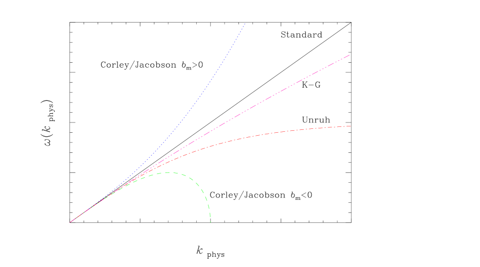
Figure 2: Various dispersion relations considered in the literature (see Refs. Unruh ; CJ ; KG , and also Ref. Mersini for another dispersion relation not displayed on the plot). For $k_{\rm phys}\ll k_{{}_{\rm C}}=k_{{}_{\rm Pl}}$, all the dispersion relations are linear, $\omega_{\rm phys}\simeq k_{\rm phys}$, which guarantees that the laws of physics on scales below the Planck scale are the standard ones. On the other hand on very small scales, for $k_{\rm phys}\gg k_{{}_{\rm C}}$, the dispersion relations deviate from the standard one.

The modification envisaged in Refs. Ve ; GM ; ACV ; GKP amounts to choose

$$[\hat{x},\hat{p}]=i\hbar(1+\beta\hat{p}^{2}),$$ (33)

which introduces a short distance cut-off. Its implications for the wave equation were studied in Ref. kempf . It has been argued that this commutation relation could be a generic prediction of string theory. It has been shown in Refs. Chu ; Easther ; kempfN that significant effect on the power spectrum are possible in this case.

The third proposal consists in assuming that the quantum state in which the cosmological perturbations are placed is no longer the vacuum but some excited state. In this case, it has been shown in Ref. Hui that a possible observable signature is the modification of the consistency relations between the spectral indices of scalar and tensor fluctuations in inflation. Proposals 2 and 3 are not necessarily unrelated. For example, in the work of Ref. Easther , the modified commutation relation leads to a state at Hubble radius crossing which is not the adiabatic vacuum.

Very recently, a fourth possibility has been suggested in Ref. Kaloper using general effective field theory techniques. In this case, it has been demonstrated that trans-Planckian effects on CMB anisotropies in an inflationary Universe are suppressed by a factor of $(H/M)^{2}$, where $H$ is the Hubble constant during inflation, and $M$ is the scale of trans-Planckian physics. If we take into account that the value of $H$ during inflation is bounded from above due to the observational bounds on the spectrum of gravitational waves Hbound , then - in models in which the string scale is close to the usual four-dimensional Planck scale - this suppression factor render the signatures of this kind of trans-Planckian physics far too small to be observed in the near future. On this basis, the authors of Ref. Kaloper conclude that short distance physics cannot be observed in the CMB. However, this conclusion clearly rests on the type of modifications chosen by the authors and is not true in general.

To demonstrate that a priori significant changes in the inflationary predictions are possible, let us come back to the case where the standard dispersion is modified. The method is to replace the linear dispersion relation $\omega_{{}_{\rm phys}}=k_{\rm phys}$ by a non standard dispersion relation $\omega_{{}_{\rm phys}}=\omega_{{}_{\bf phys}}(k)$. In the context of cosmology, it has been shown in Ref. MB that this amounts to replacing $k^{2}$ appearing in (13) with $k_{\rm eff}^{2}(n,\eta)$ defined by

$$k^{2}\,\rightarrow\,k_{\rm eff}^{2}(k,\eta)\equiv a^{2}(\eta)\omega_{{}_{\rm phys}}^{2}\biggl{[}\frac{k}{a(\eta)}\biggr{]}.$$ (34)

For a fixed comoving mode, this implies that the dispersion relation becomes time-dependent. Therefore, the equation of motion of the quantity $v_{k}(\eta)$ takes the form

$$v_{k}^{\prime\prime}+\biggl{[}k_{\rm eff}^{2}(k,\eta)-{{a^{\prime\prime}}\over a}\biggr{]}v_{k}\,=\,0\,.$$ (35)

Let us remark that a more rigorous derivation of this equation, based on a variational principle, has been provided in Ref. LLMU , see also Refs. jacobson ; jacobson2 .

The evolution of modes thus must be considered separately in three phases, see Fig. 1. In Phase I the wavelength is smaller than the Planck scale, and trans-Planckian physics is expected to play an important role. In Phase II, the wavelength is larger than the Planck scale but smaller than the Hubble radius. In this phase, trans-Planckian physics is expected to have a negligible effect (and the work of Kaloper makes this statement quantitative). Hence, by the analysis in Section II, the wavefunction of fluctuations is oscillating in this phase,

$$v_{k}\,=\,B_{1}\exp(-ik\eta)+B_{2}\exp(ik\eta)$$ (36)

with constant coefficients $B_{1}$ and $B_{2}$. In the standard approach, the initial conditions are fixed in this region and the usual choice of the vacuum state leads to $B_{1}=1/\sqrt{2k}$, $B_{2}=0$ (see the previous section). Phase III starts at the time $t_{\rm H}(k)$ when the mode crosses the Hubble radius. During this phase, the wavefunction is squeezed and is given by

$$v_{k}\,=\,C_{1}z(\eta)+C_{2}z(\eta)\int^{\eta}\frac{{\rm d}\tau}{z^{2}(\tau)}\,.$$ (37)

The source of trans-Planckian effects on observations studied in MB is the possible non-adiabatic evolution of the wavefunction during Phase I. If this occurs, then it is possible that the wavefunction of the fluctuation mode is not in its vacuum state when it enters Phase II and, as a consequence, the coefficients $B_{1}$ and $B_{2}$ are no longer given by the standard expressions above. In this case, the wavefunction will not be in its vacuum state when it crosses the Hubble radius, and the final spectrum will be different. In general $B_{1}$ and $B_{2}$ are determined by the matching conditions between phase I and II. If the dynamics is adiabatic throughout (in particular if the $a^{\prime\prime}/a$ term is negligible), the WKB approximation holds and the solution is always given by

$$v_{k}(\eta)\,\simeq\,\frac{1}{\sqrt{2k_{\rm eff}(k,\eta)}}\exp\biggl{[}-i\int_{\eta_{\rm i}}^{\eta}k_{\rm eff}{\rm d}\tau\biggr{]}\,,$$ (38)

where $\eta_{i}$ is some initial time. Therefore, if we start with a positive frequency solution only and uses this solution, one finds that no negative frequency solution appears. Deep in the region II where $k_{\rm eff}\simeq k$ the solution becomes

$$v_{k}(\eta)\simeq{1\over{\sqrt{2k}}}\exp(-i\phi-ik\eta),$$ (39)

i.e. the standard vacuum solution times a phase which will disappear when we calculate the modulus. The phase $\phi$ is given by $\phi\equiv\int_{\eta_{\rm i}}^{\eta_{1}}k_{\rm eff}{\rm d}\tau$, where $\eta_{1}$ is the time at which $k_{\rm eff}\simeq k$. By focusing only on trans-Planckian effects on the local vacuum wave function at the time $t_{\rm H}(k)$, the authors of Kaloper miss this important potential source of trans-Planckian signals in the CMB.

It is possible to give the conditions for violation of adiabaticity and to quantify exactly the accuracy of the WKB approximation. Given an equation of the form $\mu^{\prime\prime}+\omega^{2}\mu=0$ (in the present context, one has $\omega^{2}=k^{2}_{\rm eff}-a^{\prime\prime}/a$), the WKB approximation is valid if the quantity $|Q/\omega^{2}|\ll 1$, where the quantity $Q$ is defined by the following expression

$$Q=\frac{3(\omega^{\prime})^{2}}{4\omega^{2}}-\frac{\omega^{\prime\prime}}{2\omega}.$$ (40)

This standard criterion can be obtained in the following manner. The WKB solution, $\mu_{\rm wkb}$, satisfies the equation $\mu_{\rm wkb}^{\prime\prime}+\mu_{\rm wkb}(\omega^{2}-Q)=0$ exactly. Therefore, one has $\mu\simeq\mu_{\rm wkb}$ if $|Q/\omega^{2}|\ll 1$. To obtain a modification of the inflationary spectrum, it is sufficient to find a dispersion relation such that $|Q/\omega^{2}|\gg 1$ in phase I.

Let us now present some concrete examples where a change in the inflationary spectrum has been obtained. The first dispersion relation for which these effects were found is

$$k_{\rm eff}^{2}(k,\eta)=k^{2}-k^{2}|b_{m}|\biggl{[}{{\ell_{{}_{\rm C}}}\over{\lambda(\eta)}}\biggr{]}^{2m},$$ (41)

where $\lambda(\eta)=2\pi a(\eta)/k$ is the wavelength of a mode. For this case, it was found that the spectral index is modified and that superimposed oscillations appear. However, important concerns regarding the previous conclusion can be raised. For example, the dispersion relation (41) used leads to complex frequencies in the context of an inflationary model with a long period of superluminal expansion. Furthermore, the initial conditions for the Fourier modes of the fluctuation field have to be set in the region where the evolution is non-adiabatic and the use of the usual vacuum prescription can be questioned. For this reason, the previous example is not satisfactory MB2 .

Examples where a modification can be obtained without the previous difficulties can nevertheless be obtained. In Ref. LLMU such an example has been explicitly constructed with the dispersion relation

$$\omega_{\rm phys}^{2}=k^{2}_{\rm phys}+2b_{11}k_{\rm phys}^{4}-2b_{12}k_{\rm phys}^{6}.$$ (42)

The coefficients $b_{11}$ and $b_{12}$ can be chosen such the dispersion relation has a maximum around $k_{{}_{\rm C}}$ and a minimum at a scale smaller than $k_{{}_{\rm C}}$. This minimum can be chosen to be smaller than the Hubble parameter during phase I. This is the case in Fig. 3.

Figure 3: Example of a dispersion relation where the WKB approximation can be violated during phase I.

In this example, $\omega_{\rm phys}$ always remains real, the initial conditions can be fixed in a region where the WKB approximation is valid (as a consequence, the initial state can be chosen as the minimal energy state Brown78 ) and where the mode function $v_{k}$ oscillates. Since there is a phase during which the WKB approximation is not valid, the final spectrum is modified. It has been calculated explicitly in Ref. LLMU . The difficulties described previously can also be avoided by considering the evolution of fluctuations in a bouncing cosmology in which the initial conditions can be set in the asymptotically flat past, and focusing on modes for which the frequency never becomes complex BJM . For all the examples where everything can be done consistently, the coefficients $B_{1}(k)$ and $B_{2}(k)$, see Eq. (36), in phase II are found to be of the form

$$B_{1}(k) = \frac{1}{\sqrt{2k}}[1+\epsilon\xi_{1}(k)+{\cal O}(\epsilon^{2})]\,,$$ (43)

$$B_{2}(k) = \epsilon\xi_{2}(k)+{\cal O}(\epsilon^{2})\,,$$ (44)

where the functions $\xi_{1}(k)$ and $\xi_{2}(k)$ have been explicitly calculated in Refs. LLMU ; BJM . In the previous relations, $\epsilon$ is a small parameter which is basically the time that the mode has spent in the region where the WKB approximation is violated. The advantage of expanding the two coefficients in the parameter $\epsilon$ is that general equations can be obtained. But this does not mean that the correction has to be proportional to a small parameter and large non perturbative effects can also be obtained if the time spent by the mode in the region where WKB is not valid is large.

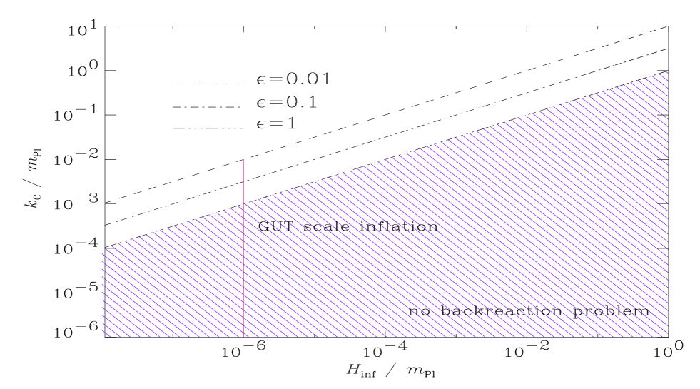
Figure 4: Region in the $(k_{{}_{\rm C}},H_{\rm inf})$ plan where a correction of order $\epsilon$ is expected with a back-reaction problem. The shaded region indicates the region obtained for $\epsilon=0.01$. For larger $epsilon$ the shaded region should be extended up to the corresponding straight line indicated on the figure.

In this case, another concern Tanaka ; Starob is that the excitations produced during Phase I might have an important back-reaction effect. This is because an excited state leads to an energy density that could be larger that the vacuum energy density causing inflation. The energy density due to trans-Planckian effect is LLMU

$$\rho\simeq{\cal O}(\epsilon^{2}k_{{}_{\rm C}}^{4}).$$ (45)

Therefore, there is no back-reaction problem if $\rho<m_{\rm Pl}^{2}H_{\rm inf}^{2}$. Obviously, the smallest $\epsilon$ is, the less severe the back-reaction problem is but, at the same time, the less important the modification of the spectrum is. The important point is that, by playing with the quantities $H_{\rm inf}$ and $k_{{}_{\rm C}}$, a window where the correction is significant and where there is no back-reaction can be found. These results are summarized in Fig. 4.

In the light of the work of Refs. Easther ; kempfN , another way to think about the coefficients $B_{1}(k)$ and $B_{2}(k)$, see Eqs. (43) and (44), is as phenomenological parameters which describe the effects of short distance physics. Trans-Planckian (stringy) physics can lead to non-standard values of these coefficients at the earliest time when the fluctuation modes can be described by the usual actions for linearized gravitational fluctuations discussed in Section II, and the work of Ref. Easther presents a concrete model where values of $B_{1}(k)$ and $B_{2}(k)$ arise which differ from the standard values enough to produce measureable effects but for which the back-reaction of the non-vacuum state at Hubble radius crossing is negligible (We thank Brian Greene for communications on this point).

IV Discussion and Conclusion

Based on a review of the theory of cosmological fluctuations as applied to inflationary cosmology we have discussed the main sources of expected trans-Planckian (stringy) signatures on the spectrum of CMB anisotropies. One important potential source MB is the fact that the evolution of the fluctuation modes can be non-adiabatic when their wavelength is smaller than the Planck (string) scale. This leads to an excited state of the fluctuation modes at the time when the mode crosses the Hubble radius at $t_{\rm H}(k)$. Another way in which trans-Planckian effects can lead to an excited state of the fluctuation modes at $t_{\rm H}(k)$ is that new physics Easther ; kempfN will generate non-trivial Bogoliubov coefficients $B_{1}(k)$ and $B_{2}(k)$, see Eqs. (43) and (44), at the earliest time that the modes can be adequately approximated by the usual actions for linearized gravitational fluctuations.

The recent paper Kaloper does not address this issue. It focuses on the computation of the trans-Planckian (stringy) corrections to the fluctuation amplitude in the local vacuum state at $t_{\rm H}(k)$, and comes to the correct conclusion that these corrections are usually negligible. If one were to try to use the effective field theory techniques used in Kaloper to address the evolution of the modes in Phase I, one would not be able to integrate over degrees of freedom with frequency larger than $H$. Since the frequencies of the modes in Phase I are trans-Planckian, one is not allowed to integrate out any sub-Planckian modes. From this point of view one would reach the conclusion that one is not in the regime of applicability of effective field theory, and that therefore the corrections to results obtained (like the standard results of inflation on the spectrum of fluctuations) should be expected to be of order unity or larger.

We hope that the review of the theory of cosmological perturbations presented in Section II will be of use to physicists not actively working on cosmological perturbations, and that it will dispel the myth that fluctuations are generated at Hubble radius crossing. Note also that in the modern version of the theory of cosmological perturbations presented here, there is no need for ad hoc ultraviolet subtractions, since the analysis is done consistently in momentum space in linear perturbation theory. A final caveat, however, is that if it were to turn out that inflation is the result of some highly nonlinear theory at a scale much smaller than the Planck scale (see e.g. the model of BZ ), then the theory of cosmological perturbations presented in Section II would not apply on scales smaller than the Hubble radius. One would then need to calculate in terms of an effective field theory, and by the analysis of Kaloper one would not expect any deviations from the expected spectrum of scale-invariant fluctuations due to trans-Planckian physics.

Acknowledgments

We would like to thank Brian Green and Paul Windey for comments and careful reading of the manuscript and the authors of Ref. Kaloper for sending us a draft of their paper before publication and for useful comments on this manuscript. We acknowledge support from the BROWN-CNRS University Accord and are grateful to Herb Fried for his efforts to secure this Accord. R. B. wishes to thank the CERN Theory Division for hospitality and support during the time when this paper was written. The research was also supported in part (at Brown University) by the U.S. Department of Energy under Contract DE-FG02-91ER40688, TASK A.

References

- (1) N. Kaloper, M. Kleban, A. Lawrence and S. Shenker, hep-th/0201158.
- (2) R. H. Brandenberger, Proceeding of the International School on Cosmology, Kish Island, Iran (2000), hep-ph/9910410.
- (3) A. Guth, Phys. Rev. D23 (1981) 347; A. Linde, Phys. Lett. B108 (1982) 389; A. Albrecht and P. J. Steinhardt, Phys. Rev. Lett. 48 (1982) 1220; A. Linde, Phys. Lett. B129 (1983) 177; A. A. Starobinsky, Pis’ma Zh. Eksp. Teor. Fiz. 30 (1979) 719 [JETP Lett. 30 (1979) 682]; V. Mukhanov and G. Chibisov, JETP Lett. 33 (1981) 532; S. Hawking, Phys. Lett. B115 (1982) 295; A. A. Starobinsky, Phys. Lett. B117 (1982) 175; J. M. Bardeen, P. J. Steinhardt, and M. S. Turner, Phys. Rev. D28 (1983) 679; A. Guth and S. Y. Pi, Phys. Rev. Lett. 49 (1982) 1110.
- (4) A. Linde, “Particle Physics and Inflationary Cosmology”, Harwood Academic, Chur, (1990).
- (5) R. H. Brandenberger and J. Martin, Mod. Phys. Lett. A16, 999 (2001), astro-ph/0005432; J. Martin and R. H. Brandenberger, Phys. Rev. D63, 123501 (2001), hep-th/0005209.
- (6) J. C. Niemeyer, Phys. Rev. D63, 123502 (2001), astro-ph/0005533; J. C. Niemeyer, astro-ph/0201511.
- (7) W. Unruh, Phys. Rev. D51, 2827 (1995).
- (8) S. Corley and T. Jacobson, Phys. Rev. D54, 1568 (1996), hep-th/9601073; S. Corley, Phys. Rev. D57, 6280 (1998), hep-th/9710075.
- (9) J. Martin and R. H. Brandenberger, Proceedings of the Ninth Marcel Grossmann Meeting on General Relativity, edited by R. T. Jantzen, V. Gurzadyan and R. Ruffini, World Scientific, Singapore, 2002, astro-ph/0012031.
- (10) J. C. Niemeyer and R. Parentani, Phys. Rev. D64, 101301 (2001), astro-ph/0101451.
- (11) A. Kempf, Phys. Rev. D63 (2001) 083514, astro-ph/0009209.
- (12) C. S. Chu, B. R. Greene and G. Shiu, Mod. Phys. Lett. A16, 2231 (2001), hep-th/0011241.
- (13) R. Easther, B. R. Greene, W. H. Kinney and G. Shiu, Phys. Rev. D64, 103502 (2001), hep-th/0104102; R. Easther, B. R. Greene, W. H. Kinney and G. Shiu, hep-th/0110226.
- (14) A. Kempf and J. C. Niemeyer, Phys. Rev. D64, 103501 (2001) astro-ph/0103225.
- (15) L. Hui and W. H. Kinney, astro-ph/0109107.
- (16) R. H. Brandenberger and P. M. Ho, in preparation.
- (17) L. Parker, Phys. Rev. 183, 1057 (1969).
- (18) N. D. Birrell and P. C. W. Davies, “Quantum fields in curved space”, Cambridge Univ. Press, Cambridge, (1982).
- (19) V. F. Mukhanov, H. A. Feldman, R. H. Brandenberger, Phys. Rept. 215, 203 (1992).
- (20) J. Martin and D. J. Schwarz, Phys. Rev. D57, 3302 (1998), gr-qc/9704049.
- (21) A. Liddle and D. Lyth, “Cosmological inflation and large-scale structure, Cambridge Univ. Press, Cambridge, (2000).
- (22) V. F. Mukhanov, Sov. Phys. JETP Lett. 41, 493 (1985), [Pisma Zh. Eksp. Teor. Fiz. 41, 402 (1985)].
- (23) V. Lukash, Sov. Phys. JETP 52, 807 (1980).
- (24) D. H. Lyth, Phys. Rev. D31, 1792 (1985).
- (25) V. F. Mukhanov, Sov. Phys. JETP 67, 1297 (1988), [Zh. Eksp. Teor. Fiz. 94, 1 (1988)].
- (26) L. P. Grishchuk, Sov. Phys. JETP 40, 409 (1975), [Zh. Eksp. Teor. Fiz. 67, 825 (1974)].
- (27) J. Kowalski-Glikman, Phys. Lett. B499, 1 (2001), astro-ph/0006250.
- (28) L. Mersini, M. Bastero-Gil and P. Kanti, Phys. Rev. D64, 043508 (2001), hep-ph/0101210.
- (29) G. Veneziano, Europhys. Lett. 2, 199 (1986).
- (30) D. Gross and P. Mende, Nucl. Phys. B303, 407 (1988).
- (31) D. Amati, M. Ciafaloni and G. Veneziano, Phys. Lett. B216, 41 (1989).
- (32) R. Guida, K. Konishi and P. Provero, Mod. Phys. Lett. A6, 1487 (1991).
- (33) V. A. Rubakov, M. V. Sazhin and A. V. Veryaskin, Phys. Lett. B115, 189 (1982); L. F. Abbott and M. B. Wise, Nucl. Phys. B244, 541 (1984).
- (34) M. Lemoine, M. Lubo, J. Martin and J. P. Uzan, Phys. Rev. D65, 023510 (2002), hep-th/0109128.
- (35) T. Jacobson and D. Mattingly, gr-qc/0007031.
- (36) T. Jacobson and D. Mattingly, Phys. Rev. D63, 041502 (2001), gr-qc/0007031.
- (37) J. Martin and R. H. Brandenberger, hep-th/0201189.
- (38) M. Brown and C. Dutton, Phys. Rev. D18, 4422 (1978).
- (39) R. H. Brandenberger, S. E. Joras and J. Martin, hep-th/0112122.
- (40) T. Tanaka, astro-ph/0012431.
- (41) A. A. Starobinsky, Sov. Phys. JETP Lett. 73, 371 (2001), [Pisma Zh. Eksp. Teor. Fiz. 73, 415 (2001)], astro-ph/0104043.
- (42) R. H. Brandenberger and A. R. Zhitnitsky, Phys. Rev. D55, 4640 (1997), hep-ph/9604407.