Soliton Decay in Coupled System of Scalar Fields

Abstract

A system of coupled scalar fields is introduced which possesses a spectrum of massive single-soliton solutions. Some of these solutions are unstable and decay into lower mass stable solitons. Some properties of the solutions are obtained using general principles including conservations of energy and topological charges. Rest energies are calculated via a variational scheme, and the dynamics of the coupled fields are obtained by solving the field equations numerically.

I Introduction

Relativistic solitons, including those of the conventional sine-Gordon equation, exhibit remarkable similarities with classical particles. They exert short range forces on each other and make collisions, without losing their identities a1 . They are localized objects and do not disperse while propagating in the medium. Because of their wave nature, they do tunnel a barrier in certain cases, although this tunnelling is different from the well-known quantum version a2 . Topological solitons are stable, due to the boundary conditions at spatial infinity. Their existence, therefore, is essentially dependent on the presence of degenerate vacua a33 .

Topology provides an elegant way of classifying solitons in various sectors according to the mappings between the degenerate vacua of the field and the points at spatial infinity. For the sine-Gordon system in 1+1 dimensions, these mapping are between $\phi=2n\pi$, $n\in\mathbb{Z}$ and $x=\pm\infty$, which correspond to kinks and anti-kinks of the SG system. More complicated mappings occur in solitons in higher dimensions. For example, in cosmic strings, the vacuum is $S^{1}$ and topological sectors corresponds to distinct mappings between this $S^{1}$ and a large circle around the string. This leads to the homotopy group $\pi^{1}(S^{1})=\mathbb{Z}$.

Coupled systems of scalar fields have been investigated by many authors bas ; riz2 ; a4 . Bazeia et al. bas considered a system of two coupled real scalar fields with a particular self-interaction potential such that the static solutions are derivable from first order coupled differential equations. Riazi et al. riz2 employed the same method to investigate the stability of the single soliton solutions of a particular system of this type. Inspired by the well-known properties of sine-Gordon equation, we introduce a coupled system of two real scalar fields which shows a considerably reacher structure and dynamics. The present system is not of the form investigated in bas and riz2 and static solutions are not derivable from first order differential equations.

In our proposed system, a spectrum of solitons with different rest energies exist which are stable, unstable or meta-stable, depending on their energies and boundary conditions. Some of the more massive solitons decay spontaneously into stable ones which subsequently leave the interaction area. Note that the term “soliton” is used throughout this paper for localized solutions. The problem of integrability of the model is not addressed here. Such non-dispersive solutions are called “lumps” by Coleman a5 to avoid confusion with true solitons of integrable models. However, it has now become popular to use the term soliton in its general sense.

Pogosian po1 investigated kink solutions in bi-dimensional $SU(N)\times Z_{2}$ models. He found that heavier kinks tend to break up into lighter ones. Comparing our results with those reported by Pogosian, it is interesting to note that fairly similar phenomena are observed in quite different systems. In an earlier paper, Pogosian and Vachaspati po2 reported $(N+1)/2$ distinct classes of kink solutions in an $SU(N)\times Z_{2}$ field theory.

The organization of the paper is as follows: In section II, we introduce the lagrangian density, dynamical equations, and conserved currents of the proposed model. In section III, some exact solutions, together with the corresponding charges and energies are derived. The necessary nomenclature, and general behavior of the solutions due to the boundary conditions are also introduced in this section. Numerical solutions corresponding to different boundary conditions are presented, and properties of these solutions like their charges, masses and their stability status are addressed in this section. In order to investigate the stability of the numerical solutions, their evolution are worked out numerically. The dynamical evolution of the unstable solutions are investigated further in section IV. Our final conclusion and a summary of the results is given in the last section.

II Dynamical Equations and Conserved Currents

Our choice of the Lagrangian density reads

$${\cal L}=\frac{1}{2}\partial^{\mu}\phi_{1}\partial_{\mu}\phi_{1}-\alpha_{1}({\phi_{2}}^{2}+\epsilon_{1})(1-cos\phi_{1})+\frac{1}{2}\partial^{\mu}\phi_{2}\partial_{\mu}\phi_{2}-\alpha_{2}({\phi_{1}}^{2}+\epsilon_{2})(1-cos\phi_{2})$$ (1)

in which $\alpha_{1,2}$ and $\epsilon_{1,2}$ are positive constants, and $\phi_{1,2}$ are two real scalar fields. The background space-time is assumed to have the metric $g_{\mu\nu}=\mathrm{diag}(1,-1)$ in 1+1 dimensions and $c=1$ has been used throughout this paper. Recall that the sine-Gordon Lagrangian density

$${\cal L}=\frac{1}{2}\partial^{\mu}\phi\partial_{\mu}\phi-\alpha(1-\cos\phi)$$ (2)

leads to single soliton solutions

$$\phi=2n\pi\pm 4\tan^{-1}e^{\sqrt{\alpha}x}$$ (3)

all having rest energies $8\sqrt{\alpha}$. Our proposed Lagrangian density (1) comes from the idea of mixing two scalar fields in such a way that the discrete vacua at $\phi_{1}=2n\pi$, $\phi_{2}=2m\pi$ ($m,n\in\mathbb{Z}$) survive, while the rest energies of solitons for each field (say $\phi_{1}$) is affected by the value of the other ($\phi_{2}$) and vice versa. It will be seen later, that this idea leads to the appearance of non-degenerate solitons with distinct topological charges.

The corresponding equations of motion are easily obtained by applying the variational principle $\delta\big{(}\int{\cal L}d^{2}x\big{)}=0$ to the lagrangian density (1):

$$\square\phi_{1}=\alpha_{1}({\phi_{2}}^{2}+\epsilon_{1})\sin\phi_{1}+2\alpha_{2}\phi_{1}(1-\cos\phi_{2}),$$ (4)

and

$$\square\phi_{2}=\alpha_{2}({\phi_{1}}^{2}+\epsilon_{2})\sin\phi_{2}+2\alpha_{1}\phi_{2}(1-\cos\phi_{1}).$$ (5)

Since the lagrangian density (1) is Lorentz invariant, the corresponding energy-momentum tensor a3

$$T^{\mu\nu}=\partial^{\mu}\phi_{1}\partial^{\nu}\phi_{1}+\partial^{\mu}\phi_{2}\partial^{\nu}\phi_{2}-g^{\mu\nu}{\cal L},$$ (6)

satisfies the conservation law

$$\partial_{\mu}T^{\mu\nu}=0.$$ (7)

The Hamiltonian density is obtained from Eq. (6) according to

$${\cal H}=T^{0}_{0}=\frac{1}{2}\dot{\phi_{1}}^{2}+\frac{1}{2}\dot{\phi_{2}}^{2}+\frac{1}{2}{{\phi^{\prime}}_{1}}^{2}+\frac{1}{2}{{\phi^{\prime}}_{2}}^{2}+V(\phi_{1},\phi_{2}),$$ (8)

where dot and prime denote time and space derivatives, respectively. It is seen from (1) that the potential is

$$V(\phi_{1},\phi_{2})=\alpha_{1}({\phi_{2}}^{2}+\epsilon_{1})(1-\cos\phi_{1})+\alpha_{2}({\phi_{1}}^{2}+\epsilon_{2})(1-\cos\phi_{2}).$$ (9)

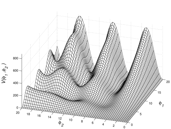
Figure 1: The self-interaction potential is shown as a height diagram over the $(\phi_{1},\phi_{2})$ plane.

This potential is shown in Fig. (1), as a height diagram over the $(\phi_{1},\phi_{2})$ plane. In this figure and any numerical calculation throughout this paper, we fix the parameters as $\alpha_{1}=0.3$, $\alpha_{2}=1$, $\epsilon_{1}=0.5$, and $\epsilon_{2}=0.07$ for the sake of being definite. The classical vacua consist of points in the $(\phi_{1},\phi_{2})$ plane at which the condition $V(\phi_{1},\phi_{2})=0$ holds. Since the potential consists of two non-negative terms, it vanishes if and only if the two terms vanish simultaneously. This leads to the vacuum set of points in the $(\phi_{1},\phi_{2})$ space:

$${\cal V}=\{(\phi_{1},\phi_{2})|\phi_{1}=2m\pi\ {\rm~{}and~{}}\ \phi_{2}=2n\pi;\ \ m,n\in\mathbb{Z}\}.$$ (10)

It can be shown that the following topological currents can be defined, which are conserved independently, and lead to quantized charges:

$$J^{\mu}_{mH} = \delta_{mp}\epsilon^{\mu\nu}\partial_{\nu}\phi_{1}/2\pi$$

$$J^{\mu}_{mV} = \delta_{mq}\epsilon^{\mu\nu}\partial_{\nu}\phi_{2}/2\pi.$$ (11)

In these equations, $m$ is an integer, and the integers $p$ and $q$ are defined according to

$$p = {\rm~{}integer~{}part~{}of~{}}(\phi_{1}/2\pi)+1,$$

$$q = {\rm~{}integer~{}part~{}of~{}}(\phi_{2}/2\pi)+1.$$

The subscripts $V$ and $H$ denote “Vertical” and “Horizontal” which will be explained later. The currents $J^{\mu}_{mH,V}$ are conserved, independent of each other:

$$\partial_{\mu}J^{\mu}_{mH} = 0,$$

$$\partial_{\mu}J^{\mu}_{mV} = 0.$$ (12)

The corresponding topological charges are given by

$$Q_{mH} = \int_{-\infty}^{\infty}J^{0}_{mH}dx\;=\;\delta_{mp}\left[\phi_{1}(+\infty)-\phi_{1}(-\infty)\right]/2\pi,$$

$$Q_{mV} = \int_{-\infty}^{\infty}J^{0}_{mV}dx\;=\;\delta_{mq}\left[\phi_{2}(+\infty)-\phi_{2}(-\infty)\right]/2\pi.$$ (13)

These charges quantify the mappings between the vacua $\phi_{1,2}(\pm\infty)\in\cal{V}$ and the points at spatial infinity.

III Single Soliton Solutions

Static solutions which correspond to transitions between adjacent vacua are symbolically shown in Fig. (2).

Figure 2: Nomenclature of horizontal ($H$) and vertical ($V$) solutions according to boundary conditions. The three lightest solutions: $H_{1}^{0}$, $V_{0}^{1}$, and $H_{1}^{1}$ are stable, while $V_{1}^{1}$ and $V_{2}^{1}$ are unstable. The corresponding rest energies and charges are shown in Table 1 for our choice of parameters.

Accordingly, we call the static solutions $H$ (horizontal) and $V$ (vertical) types. We have called them ‘horizontal’ and ‘vertical’ simply because of their orientation in ($\phi_{1},\phi_{2}$) plane. Initial guesses for these solutions are obtained using the known properties of the conventional sine-Gordon equation a4 . Note that the exact solutions are not strictly horizontal or vertical lines in the ($\phi_{1},\phi_{2}$) plane. Rather, they are bent curves joining two neighboring vacuum points due to the coupling between the two scalar fields. Any finite energy solution should start and end at one of the vacuum points belonging to $\cal{V}$ (Eq. 10). Equations (4) and (5) possess the following exact single soliton solutions:

$$H^{0}_{p+1}:\qquad\phi_{1}=4\tan^{-1}\exp\left[\pm a(x-x_{0})\right]+2p\pi\quad{\rm~{}and~{}}\quad\phi_{2}=0,$$ (14)

with

$$Q_{mH}=\delta_{mp},\qquad Q_{mV}=0,$$

and

$$V_{0}^{q+1}:\qquad\ \ \quad\phi_{2}=4\tan^{-1}\exp\left[\pm b(x-x_{0})\right]+2q\pi\quad{\rm~{}and~{}}\quad\phi_{1}=0,$$ (15)

with

$$Q_{mH}=0,\qquad Q_{mV}=\delta_{mq},$$

where $p$ and $q$ are integers. Note that Eqs. (14) and (15) satisfy Eqs. (4) and (5) in the static ($\frac{\partial}{\partial t}=0$) case. In these equations, $a=\sqrt{\alpha_{1}\epsilon_{1}}$, $b=\sqrt{\alpha_{2}\epsilon_{2}}$, and $x_{0}$ is the kink position. Apart from these exact solutions, we will introduce other static solutions which are obtained numerically later. Despite the similarity of the special solutions (14) and (15) with those of sine-Gordon equation, there are profound differences between the general static solutions of the present system and SG, including non-degenerate soliton masses and instability of some of the static solutions. The rest energies of the $H$ and $V$-type solitons are obtained by integrating the corresponding Hamiltonian densities (with $\dot{\phi_{1}}=\dot{\phi_{2}}=0$) over the $x$-space. The rest energies are approximately given by:

$$H-{\rm type}:\ \ M_{H}\simeq 8\sqrt{\alpha_{1}(4\pi^{2}n^{2}+\epsilon_{1})},$$ (16)

and

$$V-{\rm type}:\ \ M_{V}\simeq 8\sqrt{\alpha_{2}(4\pi^{2}n^{2}+\epsilon_{2})},$$ (17)

where $n$ is an integer. We have written programs in the ‘MATLAB’ environment, which calculate static solutions and the dynamical evolutions from pre-specified initial conditions. The static solutions are obtained by minimizing the energy functional

$$E=\int{\cal H}dx$$ (18)

where ${\cal H}=T_{0}^{0}$ is the energy (Hamiltonian) density, using a variational procedure. The program is asked to terminate as soon as the energy converges up to a $10^{-6}$ accuracy. Inspired by the exact solutions (14) and (15), the initial guesses were taken to be of the form of the sine-Gordon solitons. These initial guesses were deformed toward the lowest energy solutions by the variational calculation. This deformation is caused by the slope of the potential function as depicted in Fig. (1). Sample solutions are shown in Fig. (3).

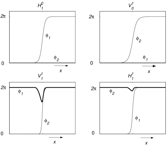
Figure 3: Examples of static solutions.

Static solutions $V^{1}_{0}$, $H^{0}_{1}$, $H^{1}_{1}$ and $V^{1}_{1}$ as projected on the ($\phi_{1}$,$\phi_{2}$) plane are shown in Fig. (4).

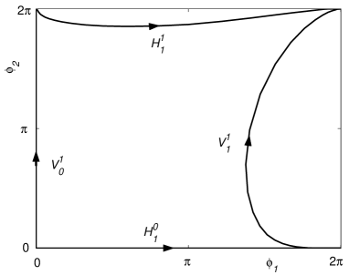
Figure 4: The static solutions $V^{1}_{0}$, $H^{0}_{1}$, $H^{1}_{1}$, and $V^{1}_{1}$ as projected on the ($\phi_{1},\phi_{2}$) plane.

A sample classification is shown in Table 1 for a particular choice of the parameters.

symbol		mass		$Q_{1H}$		$Q_{1V}$		$Q_{2H}$		$Q_{2V}$		$Q_{3H}$		stability
$V^{1}_{0}$		2.09		0		+1		0		0		0		stable
$V^{2}_{0}$		2.09		0		0		0		+1		0		stable
$H^{0}_{1}$		3.09		+1		0		0		0		0		stable
$H^{0}_{2}$		3.09		0		0		+1		0		0		stable
$H^{0}_{3}$		3.09		0		0		0		0		+1		stable
$H^{1}_{1}$		26.7		+1		0		0		0		0		stable
$H^{1}_{2}$		27.5		0		0		+1		0		0		stable
$H^{1}_{3}$		27.6		0		0		0		0		+1		stable
$V^{1}_{1}$		42.9		0		+1		0		0		0		$V^{1}_{1}\rightarrow\bar{H}^{0}_{1}V^{1}_{0}H^{1}_{1}$
$V^{2}_{1}$		48.4		0		0		0		+1		0		stable
$H^{2}_{1}$		53.6		+1		0		0		0		0		stable
$H^{2}_{2}$		54.6		0		0		+1		0		0		stable
$V^{1}_{2}$		89.6		0		+1		0		0		0		$V^{1}_{2}\rightarrow\bar{H}^{0}_{2}\bar{H}^{0}_{1}V^{1}_{0}H^{1}_{1}H^{1}_{2}$
$V^{2}_{2}$		95.5		0		0		0		+1		0		stable
$V^{1}_{3}$		129		0		+1		0		0		0		metastable

Table 1: A sample classification of the lowest energy solitons for $\alpha_{1}=0.3$, $\alpha_{2}=1$, $\epsilon_{1}=0.5$, $\epsilon_{2}=0.07$.

Anti-solitons exist with the same masses (rest energies) as solitons but with opposite charges. The anti-soliton solutions are obtained by simply exchanging the boundary conditions at $x=+\infty$ into those at $x=-\infty$. For example,

$$H_{1}^{0}:\left\{\begin{array}[]{ll}\phi_{1}(-\infty)=0,&\phi_{1}(+\infty)=2\pi\\ \phi_{2}(-\infty)=0,&\phi_{2}(+\infty)=0,\end{array}\right.$$ (19)

while

$$\bar{H}_{1}^{0}:\left\{\begin{array}[]{ll}\phi_{1}(-\infty)=2\pi,&\phi_{1}(+\infty)=0\\ \phi_{2}(-\infty)=0,&\phi_{2}(+\infty)=0.\end{array}\right.$$ (20)

It is clear from the definition of topological charges (11) that solitons and anti-solitons have opposite charges. The approximate formulae (16) and (17) may be compared with the numerical results depicted in Table 1. It can be seen that the masses of the $H$-type solitons are better approximated by Eq. (16) than those given by Eq. (17). This difference can be attributed to the fact that the horizontal solitons deviate less from the sine-Gordon solitons (see Fig.(4)).

IV Soliton Decay

The time-dependent solutions of the dynamical equations (4) and (5) were obtained numerically, by transforming these PDEs into finite difference equations, and calculating the fields $\phi_{1}(x,t)$ and $\phi_{2}(x,t)$ in successive time steps. Most of the static solutions obtained did not undergo appreciable variations when inserted into our dynamical program as initial conditions. This is a numerical indication for the stability of the corresponding static solutions. However, not all the static solutions obtained by the variational method explained in the last section were found to be stable. For the given choice of parameters, $V^{1}_{1}$, for example, is unstable and decays spontaneously via (see Fig. 5(a) and (b))

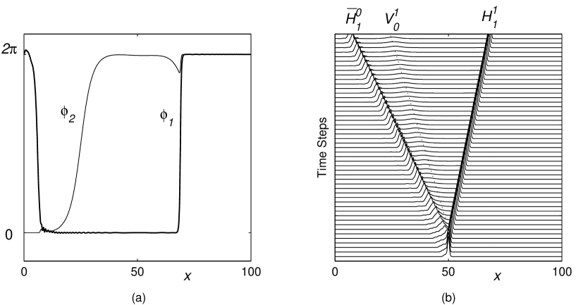
Figure 5: The decay of $V^{1}_{1}$. (a) $\phi_{1}$ and $\phi_{2}$ as a function of $x$ after the decay of $V^{1}_{1}$. (b) The energy density as a function of $x$ for various time steps. The dotted line for $V^{1}_{0}$ is added in order to clarify the trajectory of this decay product.

$$V^{1}_{1}\longrightarrow\bar{H}^{0}_{1}+V^{1}_{0}+H^{1}_{1}.$$ (21)

Here, $\bar{H}^{0}_{1}$ is the anti-soliton of $H^{0}_{1}$. Figure (5(a)) shows the $\phi_{1}$ and $\phi_{2}$ fields after several time steps. The decay product solitons can be identified at positions where the fields jump from one vacuum to an adjacent vacuum. Figure (3) helps recognizing these decay products. Figure (4) shows the stable solutions $H^{1}_{1}$, $V^{1}_{0}$, and $H^{0}_{1}$ and the unstable solution $V_{1}^{1}$ on the $(\phi_{1},\phi_{2})$ plane. Numerical calculations show that the decay of $V^{1}_{1}$ starts with the trajectory shown for this solution and evolves gradually to the $\bar{H^{0}_{1}}$ ($H^{0}_{1}$ in the reverse direction), $V_{0}^{1}$ and $H^{1}_{1}$ trajectories in this figure. Figure (5(b)) shows the corresponding energy density for various time steps. Individual solitons as decay products are more apparent in this figure.

The balance of $H$ and $V$ charges is of course respected in the decay (21), which can be easily demonstrated by computing $Q_{mV}$ and $Q_{mH}$ for $V_{1}^{1}$, $\bar{H}^{0}_{1}$, $V_{0}^{1}$, and $H_{1}^{1}$. From the conservation of energy point of view, $M(V^{1}_{1})=42.9$, while $M(\bar{H}^{0}_{1})+M(V^{1}_{0})+M(H^{1}_{1})=31.88$ which shows that the decay is allowed, and the excess energy is transferred to the kinetic energies of the solitons. As Fig. (5(b)) shows, no appreciable energy is radiated away as small amplitude wavelets.

Numerical results show that $V^{1}_{2}$ is also unstable and decays via

$$V^{1}_{2}\longrightarrow\bar{H}^{0}_{2}+\bar{H}^{0}_{1}+V^{1}_{0}+H^{1}_{1}+H^{1}_{2}.$$ (22)

Figure (6) illustrates the decay of $V^{1}_{2}$.

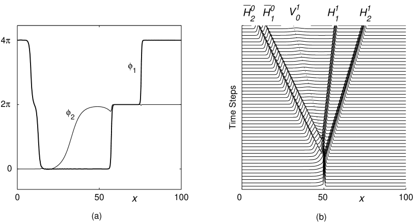
Figure 6: The decay of $V^{1}_{2}$. (a) $\phi_{1}$ and $\phi_{2}$ as a function of $x$ after the decay of $V^{1}_{2}$. (b) The energy density as a function of $x$ for various time steps.

It can be seen from Fig. (6(b)) that a $\bar{H}^{0}_{1}V^{1}_{0}H^{1}_{1}$ compound (i.e. $V_{1}^{1}$) is produced first. This compound subsequently decays into its components in a short time. Note that $M(V^{1}_{2})=89.6$ and the sum of the rest energies of the decay products is $\sum_{\mathrm{product}}M=62.47$. The difference goes to the kinetic energies of the decay products. The total energy and all topological charges are conserved. In order to demonstrate the conservation of topological charges, let us write down the charges of individual solitons:

$$V^{1}_{2} : ~{}Q_{1V}=+1~{}~{}~{}\bar{H}^{0}_{2}:~{}Q_{2H}=-1~{}~{}~{}\bar{H}^{0}_{1}:~{}Q_{1H}=-1$$

$$V^{1}_{0} : ~{}Q_{1V}=+1~{}~{}~{}H^{1}_{1}:~{}Q_{1H}=+1~{}~{}~{}H^{1}_{2}:~{}Q_{2H}=+1$$

all other charges being zero. We thus have $Q_{1V}$(LHS)=+1 and $Q_{1V}$(RHS)=+1, and all other charges equal to zero for both sides.

Surprisingly enough, although the decay of $V^{1}_{3}$ via

$$V^{1}_{3}\longrightarrow\bar{H}^{0}_{3}+\bar{H}^{0}_{2}+\bar{H}^{0}_{1}+V^{1}_{0}+H^{1}_{1}+H^{1}_{2}+H^{1}_{3}$$ (23)

is allowed by conservation of energy and charge, such a decay is not observed. We thus conclude that $V^{1}_{3}$ is a metastable soliton, and its fission needs some external trigger.

V Conclusion

Although the Sine-Gordon equation is an integrable system, even minor modifications of the equation, usually exploit its integrability. We described in this paper and elsewhere a2 ; a6 , that interesting and rich behavior may result by suitable modifications of the sine-Gordon equation irrespective of being integrable or not. Removal of mass degeneracy, soliton confinement, and soliton decay are among such properties.

For the system introduced in this paper, we presented a class of exact, single soliton solutions in the particular case where the system reduced to the sine-Gordon equation ($\phi_{1}=0$ or $\phi_{2}=0$). Other classes of static solutions were computed numerically using a variational algorithm. These static solutions were then fed into a numerical program which computed the dynamical evolution of the solution. We found that most of the static solutions were stable, while a few underwent decay into lower energy solitons. Topological charges where conserved throughout these dynamical processes, in addition to the conservation of energy and linear momentum which results from the invariance of Lagrangian under space and time translation. In the particular decay (22), two interesting effects were observed: First, the decay did not start promptly. Rather, $V^{1}_{2}$ decayed into $\bar{H}_{2}^{0}V_{1}^{1}H_{2}^{1}$ first, and $V_{1}^{1}$ decayed via (21) in a later stage. Second, the ($\bar{H}^{0}_{1},\bar{H}^{0}_{2}$) pair apparently remained as a bound system in the decay of $V^{1}_{2}$. In order to check whether $\bar{H}^{0}_{1}$ and $\bar{H}^{0}_{2}$ do form a bound system, we did numerical calculations (both variational and dynamical) for this system. It turned out that the system split into $\bar{H}^{0}_{1}$ and $\bar{H}^{0}_{2}$ which moved away from each other. We conclude that $\bar{H}^{0}_{1}\bar{H}^{0}_{2}$ do not form a bound system.

Finally, let us discuss briefly the kinematics of solitons in the decay process. Since our system is relativistic, principles of conservation of energy and momentum should be applicable in their relativistic form. Ignoring the energy and momentum radiated away in the form of small amplitude wavelets, we may write

$$Mc^{2}=\sum^{n}_{i=1}\gamma_{i}m_{i}c^{2},$$ (24)

and

$$\sum_{i=1}^{n}\gamma_{i}m_{i}v_{i}=0,$$ (25)

for the decay

$$S\rightarrow s_{1}+s_{2}+...+s_{n}.$$ (26)

In equations (24) and (25), $M$ is the mass of the $S$ soliton, $m_{i}$ are the masses of $s_{i}$ solitons, $v_{i}$ are the corresponding velocities, and $\gamma_{i}=(1-v_{i}^{2})^{-1/2}$. The system of equations (24) and (25) have a unique solution for $v_{i}$, if $n=2$. For $n>2$, we have only two equations for $n$ unknowns and the equations do not have a unique solution. However, the decay pattern and the distribution of velocities among the decay products seem to be predetermined in our numerical results (compare the decay pattern of $V_{1}^{1}$ in Figures (5) and (6)). If we note that the decay to the daughter solitons does not happen in a single stage, but rather it proceeds in successive stages, it becomes clear why the distribution of velocities among the decay products follow a unique pattern. In each stage, an unstable soliton decays into two decay products which is actually observed numerically. The velocities of the two decay products is unique, according to (24) and (25). One of the decay products, in turn, decays into two solitons in later stage, and so on.

- (1) G.L. Lamb, Jr. Elements of Soliton Theory, Wiley, New York (1980).
- (2) N. Riazi, Int. J. Theor. Phys., 35, No.1, 101 (1996).
- (3) T.D. Lee, Particle Physics and Introduction to Field Theory, Harwood, 1981.
- (4) D. Bazeia, J.R.S. Nascimento, R.F. Ribeiro and D. Toledo, J. Phys. A, 30, 8157 (1997).
- (5) N. Riazi, M.M. Golshan and K. Mansuri, Int. J. Theor. Phys. Group Theor. Non. Op., 7, No. 3, 91 (2001).
- (6) R. Rajaraman, Solitons and Instantons, North-Holland, Amsterdam (1982).
- (7) S. Coleman, in ‘New Phenomena in Subnuclear Physics’ Ed. by A. Zichichi, Plenum Press (1977).
- (8) L. Pogosian, Phys. Rev. D65, 065023 (2002).
- (9) L. Pogosian and T. Vachaspati, Phys. Rev. D64, 105023 (2001).
- (10) M. Guidry, Gauge Field Theories, An Introduction with Application, Wiley, New York (1991).
- (11) N. Riazi and A.R. Gharaati, Int. J. Theor. Phys., 37 No. 3, 1081 (1998).