$\Lambda<0$ Quantum Gravity in 2+1 Dimensions II:
Black Hole Creation by Point Particles

Using the recently proposed formalism for $\Lambda<0$ quantum gravity in 2+1 dimensions we study the process of black hole production in a collision of two point particles. The creation probability for a BH with a simplest topology inside the horizon is given by the Liouville theory 4-point function projected on an intermediate state. We analyze in detail the semi-classical limit of small AdS curvatures, in which the probability is dominated by the exponential of the classical Liouville action. The probability is found to be exponentially small. We then argue that the total probability of creating a horizon given by the sum of probabilities of all possible internal topologies is of order unity, so that there is no exponential suppression of the total production rate.

1 Introduction

In [1] we have proposed a formalism for quantum theory of asymptotically AdS 2+1 gravity. The formalism is based on the analytic continuation procedure developed in [2]. The theory is defined holographically, using a conformal field theory (CFT) on the boundary. The relevant CFT is expected to be the quantum Liouville field theory (LFT), or, more precisely, a certain extension thereof that incorporates the point particle states, see the companion paper [1] for more details.

In the present paper we apply this formalism to study black hole (BH) creation by point particles. Classically such a process was described in two papers [3, 4]. The process is essentially a $\Lambda<0$ version of the Gott time machine [5]. In this paper we obtain the quantum amplitude for black hole production. We verify the expected semi-classical behavior, in that the amplitude is peaked on the classical Matschull process.

It is important to realize that there is not one but many different classical Matschull processes. Namely, the BH created in a collision of two point particles can have a non-trivial topology inside the horizon. The process described in [3] is that corresponding to the simplest possible internal topology. In the main text we give examples of other possible internal topologies that can get created. The internal structure inside the horizon is invisible to an external observer, so is correct to think of it as the BH microstate. The formalism of [1] allows to calculate the creation probability for each internal topology (each microstate). The total probability of creating a horizon is then given by a sum of probabilities of all different possible microstates. In this paper we only study in detail the amplitude (probability) for the simplest microstate. We then give some arguments as to what the result of the sum over microstates can be.

Thus, the paper mostly deals with the process described in [3], which is the simplest one in which a horizon is created. The calculation of the amplitude for this process proceeds as follows. First we perform an analytic continuation of the classical Matschull process. The result is a particular hyperbolic 3D manifold $M$. The topology of the asymptotic boundary $\tilde{X}$ of this manifold is that of a sphere with 4 conical singularities. In a certain precise sense $\tilde{X}$ can be viewed as the double of a spatial slice $X$ of the spacetime, see below. According to the prescription [1] the Hartle-Hawking state is given by the CFT partition function on $X$, which, in our case is a disc with two conical singularities. The BH creation amplitude $\Psi$ is thus the LFT 2-point function on a disc:

$$\Psi[a;\eta,\eta]=Z_{\rm LFT}\left[\,\,\lower 16.62178pt\hbox{\psfig{height=36.135pt}}\,\,\right].$$ (1.1)

The amplitude depends on the boundary condition $a$, on the rest mass of the particles $\eta$, and on the relative position of the insertion points, which encodes the center of mass momentum of particles. This 2-point function is explicitly known, see [6]. In practice, however, we are more interested in a probability given by the amplitude squared. To obtain the probability let us take $|\Psi|^{2}$ and sum over all possible boundary conditions. Summing over boundary conditions is equivalent to “erasing” them, and the result is the 4-point function on the sphere:

$$\sum_{a}|\Psi[a;\eta,\eta]|^{2}=Z_{\rm LFT}\left[\,\,\lower 21.68121pt\hbox{\psfig{height=43.36243pt}}\,\,\right].$$ (1.2)

This quantity has the interpretation of the probability of two point particles colliding and forming a BH. To get the probability of creation of a particular size BH we have to project the 4-point function on some intermediate state. We have, schematically,

$$Z_{\rm LFT}\left[\,\,\lower 21.68121pt\hbox{\psfig{height=43.36243pt}}\,\,\right]=\sum_{P}\,\,\lower 21.68121pt\hbox{\psfig{height=43.36243pt}}$$ (1.3)

The sum here is actually an integral, see below. Each term in the sum (1.3) has the interpretation of the probability of creation of a BH of a particular size determined by the label $P$, see formula (5.7) below for a precise identification. Note that the same quantity can also be interpreted as the scattering amplitude for two point particles with the intermediate state being a BH. A determination of probability for production out of the 4-point function is standard in string theory, see, for example, a recent calculation [7] of the production rate for string balls. This once more emphasizes the “stringy” nature of this quantum theory.

The BH creation probability defined by (1.3) depends on the parameters $\eta$ (rest masses) of point particles, on the size of the BH being created, and, importantly, on the cross-ratio of the 4 insertion points on the sphere. In [1] we have stated that the cross-ratio $x$ carries information about the relative momentum of the two colliding particles. When the $x$ is complex its imaginary part encodes information about the impact parameter. In this paper we will obtain these relations. As we shall see, this is not easy, for these relations, if known, give a solution to the very hard problem of accessory parameters for uniformization of Riemann surfaces (in our case a 4-punctured sphere). We shall see that one can explicitly solve this problem for a particular Riemann surface that describes the collision of maximally massive particles. Unfortunately, this is not the most interesting case physically. However, a collision of, for example, massless particles, can still be analyzed in an important limit of a large BH created, without having an explicit solution for uniformization.

As we explain below, in the semi-classical limit of small AdS curvatures, the 4-point function is dominated by the exponential of the classical Liouville action. As it turns out, for a large BH created, the Liouville action is proportional to the BH size. Thus, we find that the probability of producing a BH of size $2\pi r_{+}$ with the simplest possible topology inside is exponentially small, and is given by:

$${\cal P}\simeq e^{-2\pi r_{+}/8G\hbar}.$$ (1.4)

This result is not surprising, because this is also the probability of a large BH exploding into a pair of point particles, a Hawking type process that is suppressed by the usual Boltzmann factor. We note that the quantity in the exponential is equal to $-\beta M/2$, where $\beta$ is the inverse temperature and $M$ is the mass of the BH of size $2\pi r_{+}$. The probability (1.4) should not be interpreted as the total probability to create a horizon, instead this is the probability to form a BH in a particular microstate (particular internal topology). A BH can be formed in other microstates. To find the total probability of creating a horizon one should sum over all possible microstates.

An argument similar to the one in [8] can be given to estimate what the result of this sum can be. Let us take for the moment, as in [8], the probability of each individual microstate to be $e^{-\beta M}$. The total number of possible BH microstates is $e^{S_{\rm BH}}$, where $S_{\rm BH}$ is the BH entropy. The point is that, unlike for the Schwarzschild BH in 3+1 dimensions, for BTZ BH the quantity $-I=S_{\rm BH}-\beta M$, where $I$ is the BH free energy, is positive: $-I>0$. This is because, for the BTZ BH, $\beta M=S_{\rm BH}/2$, unlike the Schwarzschild case $\beta M=2S_{\rm BH}$. In other words, the BTZ BH free energy is negative (like for a regular thermodynamic system), while for Schwarzschild it is positive. Thus, the argument of [8] applied to the case of 2+1 dimensions tells us that we should not expect an exponential suppression of the BH production rate: the density of states wins over the creation probability of each individual microstate. As the result (1.4) tells us, the probability of each individual microstate is even larger than that assumed in the above argument. Thus, there is even less reason to suspect a suppression in the case of 2+1 gravity. This is essentially the argument why we believe that there is no suppression. Some additional arguments are given in the last section.

The paper is mostly concerned with the original Matschull process, which describes creation of a BH of the simplest internal topology. Other possible topologies appear in section 3 and their role is emphasized in 8.

The paper is organized as follows. First, in section 2 we review the classical Matschull process. We carry out an analytic continuation of the corresponding spacetimes in section 3. Some basics of quantum LFT are reviewed in section 4. In section 5 we give an expression for the BH creation probability, and study it for the case of maximally massive particles in section 6. The probability for BH production is obtained in section 7. We conclude with a discussion.

2 The classical black hole creation process

In this section we review, in the amount needed for our purposes, the classical BH creation process. It was initially described for the case of a head-on collision of massless particles in [3], and generalized to a non-zero impact parameter in [4]. The head-on massive particles case was analyzed in paper [9].

2.1 A point particle spacetime

We start by considering a point particle that at $t=0$ moves through the origin of AdS₃. A point particle in 2+1 dimensions is described as a line of conical singularities. This line is a geodesic, it is the world-line of the particle in the spacetime, and it is also the axis of identifications. In the ${\rm SL}(2,{\mathbb{R}})$ model of AdS₃, which is briefly reviewed in the Appendix, geodesics that pass through the origin ${\bf x}={\bf e}$ are described as one-parameter subgroups of the type $e^{S{\bf n}}$, where $s\in{\mathbb{R}},{\bf n}\in{\mathfrak{s}l}(2)$. Let us parameterize the Lie algebra ${\mathfrak{s}l}(2)$ in the following way:

$${\bf n}={\bf\gamma}_{0}+\kappa{\bf\gamma}(\theta),\qquad\kappa\in{\mathbb{R}},$$ (2.1)

where $\gamma(\theta)=\gamma_{1}\sin(\theta)+\gamma_{2}\cos(\theta)$. For a timelike geodesic, which corresponds to a massive particle, $\kappa<1$. The case of a null particle corresponds to $k=1$. The exponential can be readily computed:

$$A=e^{s{\bf n}}=\cos(\pi\alpha)+{\sin(\pi\alpha)\over\sqrt{1-\kappa^{2}}}(\gamma_{0}+\kappa\gamma(\theta)),$$ (2.2)

where we have introduced

$$\pi\alpha=s\sqrt{1-\kappa^{2}}.$$ (2.3)

The set of points $e^{S{\bf n}}$ is the axis of the identification that has to be carried out to get the particle spacetime. This identification is generated by the following isometry:

$${\bf x}\to e^{s{\bf n}}{\bf x}e^{-s{\bf n}}.$$ (2.4)

It is clear that all points on the axis are left invariant under this transformation.

The spacetime obtained as the result of identifications (2.4) describes a single point particle of a particular mass. The mass can be obtained from the trace $(1/2){\rm Tr}(A)=\cos(\pi\alpha)$ of the group element generating the identifications. There are in fact two different notions of mass in AdS₃. One notion, see, e.g., [10] arises from considering a dispersion relation. One can define the particle’s momentum as the ${\mathfrak{s}l}(2)$ element that is the traceless part of $e^{s{\bf n}}$. One then gets:

$$p^{2}+\sin^{2}{\pi\alpha}=0.$$ (2.5)

It is thus natural to identify the quantity $\pi\alpha$ as the particle’s mass:

$$m=\pi\alpha.$$ (2.6)

For small $m$ the dispersion relation (2.5) is approximately that of a particle in a flat spacetime. However, $m$ close to $\pi$ again gives the dispersion relation appropriate for a small mass particle. The maximum possible mass corresponds to $m=\pi/2$. This gives the largest possible value of the norm of the momentum vector. We shall refer to such particles as maximally massive. The other notion of mass is the AdS analog of the usual ADM mass. We shall denote it by $M$ and choose it so that the AdS spacetime has zero mass. Then $M$ is related to the parameter $\alpha$ via

$$M/\pi=1-\alpha^{2}.$$ (2.7)

This relation is explained in the beginning of section 5. As it is clear from this formula, the “zero” mass particle $m=0$ has $M=\pi$ and is not the empty AdS spacetime. As we shall see later, it is actually the “zero” mass BH. One gets the empty AdS for $m=\pi$, the other “massless” case. It is important to keep in mind this double nature of mass in AdS.

2.2 Head-on collision

We are now ready to study particle collisions. We first consider the case of zero impact parameter. We take two point particles, not necessarily massless, thus generalizing the analysis of [3]. Such a more general collision has been analyzed in [9]. Note that we use a different parameterization of group elements.

For simplicity, we assume that particles have same mass. We choose the timelike geodesics –world-lines of the particles– be generated by the following two vector fields (VF):

$${\bf n}_{1}=\gamma_{0}+\kappa\gamma_{1},\qquad{\bf n}_{2}=\gamma_{0}-\kappa\gamma_{1},\qquad\kappa\leq 1.$$ (2.8)

The case of null particles considered by [3] corresponds to $\kappa=1$. One gets the generators of identifications by exponentiating the above VF’s:

$$A_{1}=e^{s{\bf n}_{1}}=\cos(\pi\alpha)+{\sin(\pi\alpha)\over\sqrt{1-\kappa^{2}}}(\gamma_{0}+\kappa\gamma_{1}),$$

$$A_{2}=e^{s{\bf n}_{2}}=\cos(\pi\alpha)+{\sin(\pi\alpha)\over\sqrt{1-\kappa^{2}}}(\gamma_{0}-\kappa\gamma_{1}).$$ (2.9)

The parameter $\pi\alpha$ is defined in (2.3). The world-lines of both particles intersect the $t=0$ plane at the origin, which gives a collision.

The result of the collision is either a point particle or a BH. The mass of the resulting object is determined by taking the trace of the product of these ${\rm SL}(2,{\mathbb{R}})$ elements. We get:

$$\cosh{\nu}=-{1\over 2}{\rm Tr}(A_{1}A_{2})=-\cos^{2}(\pi\alpha)+{1+\kappa^{2}\over 1-\kappa^{2}}\sin^{2}(\pi\alpha).$$ (2.10)

When $\nu$ is real, the result of the collision is a black hole, and $\nu$ is the half of its horizon size: $\nu=\pi r_{+}$. Let us note that the relation (2.10) between $\nu$ and the momentum $\kappa$ can be rewritten as:

$$\cosh(\nu/2)=\sin(\pi\alpha)\cosh(\mu/2).$$ (2.11)

Here the parameter $\mu$ is introduced as:

$$\cosh(\mu/2)={1\over\sqrt{1-\kappa^{2}}}.$$ (2.12)

It is now easy to determine which configurations of particles result in a BH. As is not hard to see from (2.11), a BH is created whenever $|\sin(\pi\alpha)|\cosh(\mu/2)\geq 1$. One can also rewrite this as:

$$|\cos(\pi\alpha)|\leq\kappa.$$ (2.13)

One should think of $\kappa$ as a measure of particle’s momentum. Thus, (2.13) says that a BH is created for a large enough relative momentum of particles.

The condition (2.13) is valid for massive particles only. The massless case, analyzed in [3], can be obtained by taking the limit $\kappa\to 1$. In this case the BH formation condition reduces to $s\geq 1$, which is the one obtained by Matschull.

As one can see from (2.13), there is a special value of particle’s mass for which a BH is created for any value of the momentum $\kappa$. This is when the cosine in (2.13) equals zero. This corresponds to $m=\pi/2$, which is the case of maximally massive particles. As it is clear from (2.12), the BH size is then $2\nu=2\mu$.

2.3 Non-zero impact parameter

An analysis for massless particles was given in [4]. Here we present a much simpler treatment based solely on manipulations with generators. To get the BH angular velocity we use a formula derived in [2]. Unlike in [4], we consider particles of arbitrary mass, thus generalizing results of this reference.

Let us first find a parameterization of a particle that at $t=0$ is moving through a point in AdS₃ some distance away from the origin. We will later take two such particles, thus producing a non-zero impact parameter collision. Let us consider a particle that at $t=0$ is at a point with coordinates $\rho,\varphi$. Using the formula (A.5) of the Appendix it is not hard to find that the matrix representation of this point is given by:

$${\bf x}=\cosh{\chi}+\sinh{\chi}\gamma(\varphi)=e^{\chi\gamma(\varphi)}.$$ (2.14)

Here

$$\chi=\log\left({1+\rho\over 1-\rho}\right)$$ (2.15)

is the proper distance from the origin. A geodesic passing through $\bf x$ can be obtained by a shift. Thus, let us introduce a matrix ${\bf h}=e^{\chi\gamma(\varphi)/2}$. Then a geodesic passing through $\bf x$ is obtained as a one-parameter group ${\bf h}e^{S{\bf n}}{\bf h}$, where $\bf n$ is defined in (2.1). All points on this geodesic are fixed by the isometry

$${\bf x}\to A_{L}{\bf x}A_{R}^{-1}={\bf h}e^{s{\bf n}}{\bf h}^{-1}{\bf x}{\bf h}^{-1}e^{-s{\bf n}}{\bf h}.$$ (2.16)

Let us calculate the left and right group elements generating this isometry. A straightforward but lengthy calculation gives

$$A^{L}={\bf h}e^{s{\bf n}}{\bf h}^{-1} = \cos(\pi\alpha)+{\sin(\pi\alpha)\over\sqrt{1-\kappa^{2}}}\Big{(}\sinh(\chi)\gamma(\pi/2+\varphi)+\kappa\sinh(\chi)\sin(\theta-\varphi)\gamma_{0}$$ (2.17)

$$+ \cosh(\chi)\gamma_{0}+\kappa\left(\cosh^{2}(\chi/2)\gamma(\theta)-\sinh^{2}(\chi/2)\gamma(2\varphi-\theta)\right)\Big{)}.$$

The right generator $A^{R}$ is obtained by replacing $\chi\to-\chi$. Let us now take $\theta=\pi/2,\varphi=0$. We get:

$$A_{1}^{L}=\cos(\pi\alpha)+{\sin(\pi\alpha)\over\sqrt{1-\kappa^{2}}}\Big{(}(\cosh(\chi)+\kappa\sinh(\chi))\gamma_{0}+(\kappa\cosh(\chi)+\sinh(\chi))\gamma_{1}\Big{)}.$$ (2.18)

For $\kappa=1$ (null particle) this becomes $1+s\,e^{\chi}(\gamma_{0}+\gamma_{1})$, which is the same group element as the one considered in [4]. To get the right group element one has to replace $\chi\to-\chi$. One gets:

$$A_{1}^{R}=\cos(\pi\alpha)+{\sin(\pi\alpha)\over\sqrt{1-\kappa^{2}}}\Big{(}(\cosh(\chi)-\kappa\sinh(\chi))\gamma_{0}+(\kappa\cosh(\chi)-\sinh(\chi))\gamma_{1}\Big{)}.$$ (2.19)

Few remarks are necessary about particle’s motion. First of all, when $\kappa=0$ at $t=0$ the particle is at rest at point $\bf x$. It will then start falling towards the origin along $\varphi=0$, where it will have certain momentum. Thus, the case of $\kappa=0$ and non-zero $\chi$ is the same as that of non-zero $\kappa$ and zero $\chi$, except that in the former case the particle moves through the origin at $t=\pi/2$. To compare the two cases we note that, for $\chi=0$, the maximal coordinate distance $\rho_{max}$ that the particle can move away from the origin is:

$${2\rho_{max}\over 1+\rho_{max}^{2}}=\kappa.$$ (2.20)

The particle first reaches this point at $t=\pi/2$. The corresponding proper distance from the origin is ${\rm Arccosh}(1/\sqrt{1-k^{2}})=\mu/2$, where $\mu$ is the same quantity that already appeared in (2.12). For $\mu,\chi$ both non-zero we have a particle that at $t=0$ is the proper distance $\chi$ away from the origin, and has momentum $\kappa$ in the direction orthogonal to the line $\varphi=0$. At time $t=\pi/2$ the particle is the proper distance $\mu/2$ from the origin. When $\chi>\mu/2$ one gets the same orbits only that the two parameters interchange. It is thus enough to consider only the range of parameters $\chi\leq\mu/2$.

Let us now bring the second particle. We take it to be moving in the opposite direction, which corresponds to $\theta=3\pi/2$ and passing through the point $\rho,\varphi=\pi$. The corresponding left and right generators are

$$A_{2}^{L}=\cos(\pi\alpha)+{\sin(\pi\alpha)\over\sqrt{1-\kappa^{2}}}\Big{(}(\cosh(\chi)+\kappa\sinh(\chi))\gamma_{0}-(\kappa\cosh(\chi)+\sinh(\chi))\gamma_{1}\Big{)},$$ (2.21)

$$A_{2}^{R}=\cos(\pi\alpha)+{\sin(\pi\alpha)\over\sqrt{1-\kappa^{2}}}\Big{(}(\cosh(\chi)-\kappa\sinh(\chi))\gamma_{0}-(\kappa\cosh(\chi)-\sinh(\chi))\gamma_{1}\Big{)}.$$

The result of the collision can be found by finding the left and right group elements $A^{L,R}$ generating the corresponding identification. A straightforward calculation gives:

$$\cosh\nu={1\over 2}{\rm Tr}(A^{L}) = -{1\over 2}{\rm Tr}(A_{1}^{L}A_{2}^{L})=$$ (2.22)

$$- \cos^{2}(\pi\alpha)+{\sin^{2}(\pi\alpha)\over 1-\kappa^{2}}\left((1+\kappa^{2})\cosh(2\chi)+2\kappa\sinh(2\chi)\right),$$

$$\cosh\bar{\nu}={1\over 2}{\rm Tr}(A^{R}) = -{1\over 2}{\rm Tr}(A_{1}^{R}A_{2}^{R})=$$ (2.23)

$$- \cos^{2}(\pi\alpha)+{\sin^{2}(\pi\alpha)\over 1-\kappa^{2}}\left((1+\kappa^{2})\cosh(2\chi)-2\kappa\sinh(2\chi)\right).$$

From here, using simple manipulations, we obtain:

$$\cosh(\nu/2)=\sin(\pi\alpha)\cosh(\mu/2+\chi),\qquad\cosh(\bar{\nu}/2)=\sin(\pi\alpha)\cosh(\mu/2-\chi),$$ (2.24)

where $\mu$ was defined in (2.12). We thus obtained the same relations as (2.11), where $\mu/2$ is replaced by $\mu/2+\chi$ for the left group element and by $\mu/2-\chi$ for the right one. Now the parameters of the corresponding BH can be obtained using the formulas derived in [2]. We get:

$$\pi r_{+}={1\over 2}(\nu+\bar{\nu}),\qquad\pi r_{+}\Omega=\pi r_{-}={1\over 2}(\nu-\bar{\nu}).$$ (2.25)

Let us first consider the case of two particles of the maximal mass. We then have $\sin(\pi\alpha)=1$ and, thus, as for the head-on case, a BH is created for any value of the momentum $\kappa$. The BH size is $2\pi r_{+}=2\mu$ and the angular velocity is $\Omega=2\chi/\mu$. In other words, the BH size is determined solely by the momentum $\kappa$, and is given by the same expression as in the head-on case. The impact parameter $2\chi$ is equal to a half of the inner horizon size. Let us also note that when $2\chi=\mu$ an extremal rotating BH is created. Because $\chi\leq\mu/2$ no naked singularity can be created.

The described case of particles of the maximal mass is somewhat pathological because, as is clear from a comparison of the horizon size $2\pi r_{+}=2\mu$ and of the proper distance $\mu$ between the particles at maximum separation, the horizon exists already at maximum separation. Thus, the spacetime containing two particles of maximal mass is a black hole, for the particles are always behind the horizon. For zero $\chi$, the two particles fall towards each other, collide and then hit the BH singularity. For a non-zero $\chi$ the particles never hit the singularity, oscillating between the inner and outer horizons. In particular, for the extremal case $\chi=\mu/2$, and the particles are always at the same distance from each other, just behind the horizon.

Let us now consider the other limiting case, that of massless particles. Then $\kappa\to 1$ and we get:

$$\cosh(\nu/2)=s\,e^{\chi},\qquad\cosh(\bar{\nu}/2)=s\,e^{-\chi}.$$ (2.26)

As is clear from this expressions a BH is created whenever $s\geq e^{\chi}$. Both the BH size and angular momentum can now be obtained using (2.25). It is instructive to plot $\pi r_{+},\pi r_{-}$ as functions of $\chi$ at fixed relative momentum $s$. For large $s$ the BH size is $2\pi r_{+}=2\log(4s^{2})+O(1/s^{2})$, and this is practically unchanged for the whole range of parameter $\chi\leq\log(s)$, except for a small region near $\chi=\log(s)$. At extremality the black hole size drops to $2\pi r_{+}=2\log(2s^{2})$, that is by $2\log{2}$. The dependence of the $2\pi r_{-}$ on $\chi$ is practically linear for the whole range of $\chi$. One gets, sufficiently far from extremality: $2\pi r_{-}=4\chi$. Thus, for a large relative momentum $s$, and sufficiently far from extremality, the dependence of the inner, outer horizon radii on the parameters of the colliding particles is essentially the same as in the maximally massive case. Null case gives something new only for either small momentum $s$, or close to the extremality. As we shall see, this carries over into the quantum theory. The situation of large $s$ null particles is described in the quantum theory by the same formulas as the maximally massive case.

3 Analytic continuation

Here we carry out an analytic continuation of the spacetimes of the previous section. We use the procedure described in [2], although only black hole spacetimes were treated in this reference. A generalization to point particles is somewhat non-trivial. The content of this section is new.

3.1 Zero impact parameter

We start by considering a single point particle moving at $t=0$ through the origin of AdS. Later we take two such particles moving in opposite directions to obtain a zero impact parameter collision.

In order to analytically continue the particle spacetime we, following [11, 2], consider the action of the isometry (2.4) on the conformal boundary cylinder $\cal I$. The main idea is to find and analytically continue the fixed points of this action. To this end we need to find the restriction onto $\cal I$ of the VF $\xi$ generating (2.4). To get $\xi$ we simply have to replace the $\gamma$-matrices in (2.1) by the VF’s $J_{i}$ (A.16), and then use (A.15) to restrict the result to the boundary. One has to do this separately for the right and left VF’s. We get, for the left part:

$$s{\bf n}=-2s\left(1+\kappa(\sin{u}\sin{\theta}-\cos{u}\cos{\theta})\right)\partial_{u}=-2s(1-\kappa\cos(u+\theta))\partial_{u}.$$ (3.1)

Let us note that this can be rewritten as:

$$s{\bf n}=-4s\kappa\sin{\left({u+\theta+i\delta\over 2}\right)}\sin{\left({u+\theta-i\delta\over 2}\right)}\partial_{u}=-4s\kappa\sin{\left({u-u_{p}\over 2}\right)}\sin{\left({u-u_{p^{\prime}}\over 2}\right)}\partial_{u}.$$ (3.2)

Here we have introduced

$$1/\kappa=\cos{i\delta}.$$ (3.3)

and $u_{p}=i\delta-\theta,u_{p^{\prime}}=-i\delta-\theta$. The full VF becomes:

$$\xi=-4s\kappa\sin{\left({u-u_{p}\over 2}\right)}\sin{\left({u-u_{p^{\prime}}\over 2}\right)}\partial_{u}+4s\kappa\sin{\left({v-v_{p}\over 2}\right)}\sin{\left({v-v_{p^{\prime}}\over 2}\right)}\partial_{v},$$ (3.4)

where $v_{p}=-i\delta+2\pi-\theta,v_{p^{\prime}}=i\delta-\theta$. The factor of $2\pi$ in $v_{p}$ is introduced so that the two terms on the right hand side have the opposite signs. There is some amount of ambiguity here, for one can always shift any of the null coordinates by $2\pi$. As we shall see, our choice gives the correct pattern of fixed lines for the case of a null particle.

Figure 1: The conformal boundary $\cal I$ for a null particle. Fixed lines of the VF $\xi$ are shown.

The two fixed points of the VF $\xi$ are located at $u_{p},v_{p^{\prime}}$ and $u_{p^{\prime}},v_{p}$. In other words, the $t,\phi$ coordinates are given by:

$$t=i\delta-\theta,\phi=0,\qquad t^{\prime}=-i\delta+\pi-\theta,\phi^{\prime}=\pi.$$ (3.5)

Let us see that this gives an expected pattern of fixed lines in the null case. In this case $\kappa=1$ and $\delta=0$. Let us also take $\theta=\pi/2$ for definiteness, which corresponds to the particle 1 of the previous section. We have two fixed points at $t=-\pi/2,\phi=0$ and $t^{\prime}=\pi/2,\phi^{\prime}=\pi$. The corresponding set of fixed lines is shown in Fig. 1 and is as expected, see [4].

In case of a massive particle $\kappa<1$ and $\delta\not=0$. The coordinates of the fixed points are now complex. This corresponds to the fact that massive particles never reach the boundary. Indeed, the fixed points of $\xi$ are exactly those points where particle’s world-line would intersect the boundary. Let us now go to the Euclidean cylinder, see Fig. 2. We replace $t\to it$ and map the resulting Euclidean cylinder to the $z$-plane. Fixed points of $\xi$ go to the following two points:

$$z=e^{-\delta-i\theta},\qquad z^{\prime}=e^{\delta+2\pi i-i\theta}.$$ (3.6)

From now on we will put $\theta=\pi/2$ for definiteness. We have $z=-ie^{-\delta},z^{\prime}=-ie^{\delta}$. The corresponding points on the $w$-plane are:

$$w=-{1\over\cosh{\delta}}+i{\sinh{\delta}\over\cosh{\delta}}=-\kappa+i\sqrt{1-\kappa^{2}}={-\sinh(\mu/2)+i\over\cosh(\mu/2)},$$ (3.7)

and $w^{\prime}=1/w=\bar{w}$. We note that both points lie on the unit circle, $w$ above and $w^{\prime}$ below the real axis. Note that, in case the particle is not moving $\kappa=0$ and the fixed points are $w=i,w^{\prime}=-i$. This is as expected, for these are the points that on the cylinder are at plus and minus infinity, so that the line connecting them is the axis of the cylinder. This describes a particle that is located at the center of AdS at any $t$. The other limiting case, that of a null particle, is described by both fixed points approaching the real axis.

One can repeat the above continuation procedure for the particle 2 of the previous section, for which $\theta=3\pi/2$. As one can convince oneself, to go from particle 1 to particle 2 it is enough to replace $i\delta\to i\delta+\pi$ in formulas for the fixed points. Let us denote the fixed points of the first particle by $w_{1},w_{1}^{\prime}$, with $w_{1}$ given by (3.7) and those of the second particle by $w_{2},w_{2}^{\prime}$. We take $w_{2}$ to be in the upper half-plane. We get:

$$w_{2}=\kappa+i\sqrt{1-\kappa^{2}}={\sinh(\mu/2)+i\over\cosh(\mu/2)},$$ (3.8)

and $w_{2}^{\prime}=1/w_{2}=\bar{w}_{2}$. All 4 fixed points are located on the unit circle, see Fig. 3.

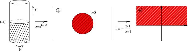
Figure 2: Analytic continuation of the boundary cylinder $\cal I$.

The analytic continuation of the spacetime in question can now be described as follows. It is a particular hyperbolic 3D manifold $M$, whose conformal boundary has the topology of a sphere with 4 conical singularities. $M$ is obtained as the quotient of the hyperbolic space ${\bf H}$ by a certain discrete group of isometries $\Sigma$. For the case in hand, $\Sigma$ is a group freely generated by two elements $L_{1},L_{2}\in{\rm SL}(2,{\mathbb{C}})$. According to the analytic continuation rule [2], the elements $L_{1},L_{2}$ must be chosen in such a way that their fixed points coincide with the obtained analytically continued fixed points $w_{1},w_{1}^{\prime},w_{2},w_{2}^{\prime}$. The trace does not change in the analytic continuation. For the considered case of particles of equal mass, and thus same parameter $\alpha$, see (2.3), $L_{1},L_{2}$ belong to the same conjugacy class:

$${1\over 2}{\rm Tr}(L_{1})={1\over 2}{\rm Tr}(L_{2})=\cos(\pi\alpha).$$ (3.9)

Since the fixed points of $L_{1}$ $w_{1},w_{1}^{\prime}$ are the complex conjugates of each other (same for $L_{2}$), the group $\Sigma$ is a discrete subgroup of ${\rm SL}(2,{\mathbb{R}})\in{\rm SL}(2,{\mathbb{C}})$.

To understand the geometry of $M$ let us describe the conformal boundary $\tilde{X}$ of $M$. We recall that the conformal boundary of the hyperbolic space ${\bf H}$ is the Riemann sphere, where the isometry group ${\rm SL}(2,{\mathbb{C}})$ acts by fractional linear transformations. The geometry of the boundary of ${\bf H}/\Sigma$ is thus that of ${\cal C}/\Sigma$ where $\cal C$ is the complement of the set of fixed points of the action of $\Sigma$ on the complex plane. To visualize this geometry it is enough to find the fundamental region. As is not hard to convince oneself, a half of the fundamental region for the group generated by $L_{1},L_{2}$ is given by a domain $D$ bounded by 4 circular arcs. The vertices of the curvilinear polygon $D$ are at the fixed points $w_{1},\bar{w}_{1},w_{2},\bar{w}_{2}$. The angles at all the vertices are $\pi\alpha$. The boundary $\tilde{X}$ of $M$ can then be pictured as two copies of $D$ glued along their boundaries to form a sphere with 4 conical singularities.

Figure 3: A half of the fundamental region for $\Sigma$ is shown: (a) for the case of particles of the maximal mass $m=\pi/2$; (b) for the null case.

The geometry of the boundary is particularly simple when we take particles of the maximal mass $m=\pi/2$. The angles at all vertices become right, and $D$ is a polygon bounded by 4 mutually orthogonal arcs, see Fig. 3(a). As is not hard to find, the radius of the two circles bounding $D$ on left and right is $\sqrt{1-k^{2}}/k$, the location of the centers on the real axis is at $\pm 1/k$.

For null particles all 4 fixed points lie on the real axis, at points $\pm 1$. The generators $L_{1},L_{2}$ become parabolic in this case. A half of the fundamental region is shown in Fig. 3(b).

To further understand the geometry of $\tilde{X}$, let us restrict our attention to the upper half-plane ${\bf U}$. The group $\Sigma\subset{\rm SL}(2,{\mathbb{R}})$ and thus acts by isometries on ${\bf U}$. A half of the fundamental region for this action is just the part of $D$ that lies above the real axis. We thus see that $X={\bf U}/\Sigma$ is a hyperbolic manifold with 2 conical singularities and one asymptotic region. The circumference $l$ of the throat of this asymptotic region can be easily computed. Half of $l$ is given by the distance in ${\bf U}$ between the arcs $w_{1},-A$ and $A,w_{2}$. As is not hard to find, $l/2=\nu$, where $\nu$ was defined in (2.11). This means that the 2D hyperbolic manifold $X={\bf U}/\Sigma$ has the geometry of 2 point particles inside the throat of size $l=2\pi r_{+}$. In other words, this is the geometry of two point particles and a BH of size $2\pi r_{+}$.

Figure 4: The geometry of ${\bf U}/\Sigma$ is that of an infinite throat ending on two conical singularities. What is shown here is the geometry for the case of particles of mass $m<\pi/2$. For the maximal mass the conical singularities are located exactly on the minimal curve $l$. In the case of null particles one gets two infinite throats of zero circumference instead of conical singularities.

As it became clear from the above discussion, the geometry of $\tilde{X}$ is that of the Schottky double of $X={\bf U}/\Sigma$. The geometry of $X$ is always that of a BH with two point particles. The size of the BH can be computed either by multiplying the holonomies in the Lorentzian signature, as we did in the previous section, or by computing the size of the throat on ${\bf U}/\Sigma$. These two different calculations give the same result. According to the prescription of [1] the amplitude of a spatial slice geometry $X={\bf U}/\Sigma$ is given by the LFT partition function on this Riemann surface. As we discussed in the introduction, the probability is given by the LFT partition function on the double $\tilde{X}={\cal C}/\Sigma$, which is a sphere with 4 conical singularities. To evaluate this partition function we will need to understand a relation between the geometry of $\tilde{X}$ and location of the points of insertion of vertex operators in the 4-point function. We will deal with this below, after we generalize the analytic continuation to the case of a non-zero impact parameter.

3.2 Rotating case

We now take two particles that are moving towards each other with some non-zero impact parameter. The analytic continuation procedure is the same as before. We need to find the VF’s that generate identifications producing the spacetime, find the restriction of these VF’s to the conformal boundary $\cal I$, and determine the fixed points. The fixed points are then to be analytically continued by maps in Fig. 2 to the complex $w$-plane. Having obtained the fixed points $w_{1},\bar{w}_{1},w_{2},\bar{w}_{2}$ on the $w$-plane one can construct a group $\Sigma\subset{\rm SL}(2,{\mathbb{C}})$ generated by, in our case, two generators, whose fixed points are $w_{1},\bar{w}_{1},w_{2},\bar{w}_{2}$. The generators are elliptic, corresponding to rotations on an angle $2\pi\alpha$. This specifies the group $\Sigma$ completely.

In practice, however, it is much easier to simply guess what the locations of the fixed points must be. Recall, see (2.11), (2.24), that to go from to the non-zero impact parameter case one had to replace $\mu/2$ by $\mu/2\pm\chi$. Recall also that $\chi$ is related to the BH angular momentum, and the later should be analytically continued as we analytically continue the spacetime. This leads to the following guess for the fixed points:

$$w_{1}={-\sinh(\mu/2+i\chi)+i\over\cosh(\mu/2+i\chi)},\qquad w_{1}^{\prime}=1/w_{1},$$ (3.10)

and

$$w_{2}={\sinh(\mu/2+i\chi)+i\over\cosh(\mu/2+i\chi)},\qquad w_{2}^{\prime}=1/w_{2}.$$ (3.11)

This guess for the fixed points can be checked, for example, by analytically continuing the resulting generators $L_{1},L_{2}$ back to the Lorentzian signature, as described in [2]. One indeed gets the isometries $A_{1},A_{2}$ given by (2.18), (2.19), (2.21). Note that the fixed points are no longer on the unit circle, and they are not complex conjugates of each other, although it is still true that $w^{\prime}=1/w$.

One can now construct a group $\Sigma$ generated by two elliptic elements $L_{1},L_{2}$ with traces satisfying (3.9), and with fixed points given by $w_{1},w_{1}^{\prime}$ and $w_{2},w_{2}^{\prime}$ correspondingly. The group $\Sigma$ is no longer a subgroup of ${\rm SL}(2,{\mathbb{R}})$. This is, of course, as expected, for the presence of rotation is generally manifested by $\Sigma$ being complex. The space ${\bf H}/\Sigma$ is a hyperbolic 3-manifold, whose conformal boundary $\tilde{X}$ has the topology of a sphere with 4 conical singularities. The boundary $\tilde{X}$ can be thought of as obtained by gluing two copies of the non-rotating case surface $X$ with a twist. We will not need any further details on the rotating case. As we saw, a non-zero impact parameter can be incorporated by simply replacing $\mu/2$ by $\mu/2+i\chi$ in all the formulas. Thus, the rotating black hole situation is obtained from the zero impact parameter case by an analytic continuation in $\mu$.

3.3 Other topologies

The purpose of this subsection is to note that, in addition to the simplest topology shown in Fig. 4, more complicated topologies of the spatial slice may appear as a result of the collision. The corresponding spacetimes may be obtained by choosing a more non-trivial group $\Gamma$.

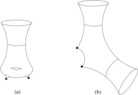
Figure 5: Other topologies that can be created inside the horizon include: (a) a torus; (b) another asymptotic region.

For example, let us consider a group $\Gamma$ generated by two elliptic elements, corresponding to the two colliding particles, and, in addition, two hyperbolic elements whose axes intersect. One gets a spacetime whose spatial slice topology is depicted in Fig. 5(a). Thus, this spacetime describes a process in which two point particles collide and form a BH with a torus inside the horizon.

Another spacetime is obtained by taking, in addition to the elliptic particle generators, two hyperbolic generators whose axes do not intersect. One obtains a spacetime with the spatial slice topology shown in Fig. 5(b) This is the spacetime describing two colliding particles that produce a BH with an asymptotic region inside.

It is now clear that one can construct spacetimes describing two colliding particles producing a BH with an arbitrary topology inside the horizon. All this topologically non-trivial structure is behind the horizon, and is thus invisible from the asymptotic region where particles lived before the collision. This structure is, in some sense, a micro-state of the BH created. It is clear that in order to find the probability of two particles forming a horizon one should sum over all possible topologies that can appear inside. We discuss such a sum in the last section.

We are now basically ready to define and study the BH creation probability. We do this in section 5, after we review some basics of Liouville theory.

4 Quantum Liouville theory

In this section we review some basic facts about the quantum LFT, in the amount we need for the following. Our main reference here is [12], see also [13] and [14].

4.1 General properties

The Liouville theory action is:

$$A_{L}[\phi]=\int d^{2}x\left[{1\over 4\pi}(\partial_{a}\phi)^{2}+\mu e^{2b\phi}\right].$$ (4.1)

Here $\phi$ is the Liouville field, $b$ is the coupling constant of the theory and $\mu$ is a constant of the dimension of $1/({\rm length})^{2}$, which sets a scale for the theory. We leave the region over which the integral is taken unspecified for now. Usually one also adds to the Lagrangian a term proportional to $\phi R$, where $R$ is the curvature scalar of a fixed background metric, and adjusts the coefficient in front of this term so that the action is independent of the background. For our purposes, however, it is more convenient to work in the flat background (this is also the choice of [12]). Then the integral of $\phi R$ translates into a set of boundary terms, see below. Although by appropriately choosing the boundary terms one can define LFT on any Riemann surface, see [15], in the present paper we are interested in LFT on the sphere. It is most convenient to work with the extended complex plane. The field $\phi$ is then required to have the following asymptotic for $|z|\to\infty$:

$$\phi(z,\bar{z})=-Q\log(z\bar{z})+O(1).$$ (4.2)

Here $Q$ is given by:

$$Q=b+{1\over b}.$$ (4.3)

To make the action (4.1) well-defined on such fields, one introduces a large disc $D$ of radius $R\to\infty$ and adds a boundary term to the action:

$$A_{L}=\int_{\Omega}d^{2}x\left[{1\over 4\pi}(\partial_{a}\phi)^{2}+\mu e^{2b\phi}\right]+{Q\over\pi R}\int_{\partial\Omega}dl\,\phi+2Q^{2}\log{R}.$$ (4.4)

The last term is needed to make the action finite as $R\to\infty$.

The vertex operators of LFT are:

$$V_{\zeta}(z)=e^{2\zeta\phi(z)},$$ (4.5)

where $z$ is a point on $S^{2}$. They are primary operators of conformal dimension:

$$\Delta_{\zeta}=\zeta(Q-\zeta).$$ (4.6)

Correlation functions of vertex operators are formally defined as the following functional integral:

$${\cal G}_{\zeta_{1},\ldots,\zeta_{n}}(z_{1},\ldots,z_{n})=\int{\cal D}\phi\,V_{\zeta_{1}}(z_{1})\cdots V_{\zeta_{n}}(z_{n})e^{-A_{L}[\phi]}.$$ (4.7)

The integral must be taken over the fields satisfying the boundary condition (4.2).

The scale dependence of correlators is:

$${\cal G}_{\zeta_{1},\ldots,\zeta_{n}}(z_{1},\ldots,z_{n})=(\pi\mu)^{(Q-\sum\zeta_{i})/b}F_{\zeta_{1},\ldots,\zeta_{n}}(z_{1},\ldots,z_{n}),$$ (4.8)

where $F_{\zeta_{1},\ldots,\zeta_{n}}(z_{1},\ldots,z_{n})$ is independent of the scale $\mu$.

The spectrum of LFT consists of the states created by $V_{\zeta}$ with

$$\zeta={Q\over 2}+iP.$$ (4.9)

These are the normalizable states. One can also consider the “states” created by $V_{\zeta}$ with $0<\zeta<Q$. These operators create conical singularities and thus correspond to non-normalizable states.

4.2 Three-point function

The three-point function in LFT is given by the Dorn-Otto-Zamolodchikov-Zamolodchikov (DOZZ) formula:

$${\cal G}_{\zeta_{1},\zeta_{2},\zeta_{3}}(z_{1},z_{2},z_{3})=|z_{12}|^{2\Delta_{12}}|z_{23}|^{2\Delta_{23}}|z_{31}|^{2\Delta_{31}}C(\zeta_{1},\zeta_{2},\zeta_{3}),$$ (4.10)

where $z_{ij}=z_{i}-z_{j},\Delta_{ij}=\Delta_{k}-\Delta_{i}-\Delta_{j},i\not=k,j\not=k,\Delta_{i}=\Delta_{\zeta_{i}}$ and

$$C(\zeta_{1},\zeta_{2},\zeta_{3}) = \left[\pi\mu\gamma(b^{2})b^{2-2b^{2}}\right]^{(Q-\sum\zeta_{i})/b}\times$$ (4.11)

$$\times {\Upsilon_{0}\Upsilon(2\zeta_{1})\Upsilon(2\zeta_{2})\Upsilon(2\zeta_{3})\over\Upsilon(\zeta_{1}+\zeta_{2}+\zeta_{3}-Q)\Upsilon(\zeta_{1}+\zeta_{2}-\zeta_{3})\Upsilon(\zeta_{2}+\zeta_{3}-\zeta_{1})\Upsilon(\zeta_{3}+\zeta_{1}-\zeta_{2})}.$$

Here

$$\gamma(x)={\Gamma(x)\over\Gamma(1-x)},$$ (4.12)

and $\Upsilon(x)$ is a special function defined by the following integral representation:

$$\log\Upsilon(x)=\int_{0}^{\infty}{dt\over t}\left[\left({Q\over 2}-x\right)^{2}e^{-t}-{\sinh^{2}\left({Q\over 2}-x\right){t\over 2}\over\sinh{bt\over 2}\sinh{t\over 2b}}\right].$$ (4.13)

The quantity $\Upsilon_{0}$ is defined as:

$$\Upsilon_{0}=\left({d\Upsilon(x)\over dx}\right)_{x=0}.$$ (4.14)

4.3 4-point function

The 4-point function can be reduced to a function of the cross-ratio

$$x={z_{12}z_{34}\over z_{13}z_{24}}.$$ (4.15)

It is thus convenient to put $z_{4}=0,z_{3}=x,z_{2}=1,z_{1}=\infty$. One introduces:

$${\cal G}_{\zeta_{1},\ldots,\zeta_{4}}(\infty,1,x,0):=G_{\zeta_{1},\ldots,\zeta_{4}}(x,\bar{x}).$$ (4.16)

The 4-point function $G_{\zeta_{1},\ldots,\zeta_{4}}(x,\bar{x})$ can be decomposed into a sum over intermediate states:

$$G_{\zeta_{1},\zeta_{2},\zeta_{3},\zeta_{4}}(x,\bar{x})={1\over 2}\int_{-\infty}^{\infty}C(\zeta_{1},\zeta_{2},{Q\over 2}+iP)C(\zeta_{3},\zeta_{4},{Q\over 2}-iP)|{\cal F}(\Delta_{1},\ldots,\Delta_{4},\Delta;x)|^{2}dP.$$ (4.17)

The function ${\cal F}(\Delta_{1},\ldots,\Delta_{4},\Delta;x)$ is the so-called conformal block [16], which sums up all descendants of a given primary state. It depends on the central charge of LFT

$$c=1+6Q^{2},$$ (4.18)

and on the conformal dimension

$$\Delta={Q^{2}\over 4}+P^{2}.$$ (4.19)

4.4 Semi-classical limit

In the semi-classical limit the LFT correlators are dominated by the classical Liouville action, which appears as the $b\to 0$ limit of (4.1). One then introduces a new “classical” Liouville field:

$$\varphi=2b\phi,$$ (4.20)

The “quantum” action (4.1) is then:

$$A_{L}[\phi]={1\over b^{2}}S_{Liouv}[\varphi],$$ (4.21)

where

$$S_{Liouv}[\varphi]={1\over 8\pi}\int d^{2}x\left[{1\over 2}(\partial_{a}\varphi)^{2}+8\pi\mu b^{2}e^{\varphi}\right]$$ (4.22)

is the classical Liouville action. There are also some boundary terms to be added to this action, see below. Varying the classical action with respect to $\varphi$ one finds that locally $\varphi$ satisfies the classical Liouville equation:

$$\Delta\varphi=8\pi\mu b^{2}e^{\varphi}.$$ (4.23)

Then the metric $ds^{2}=e^{\varphi}|dz|^{2}$ is a metric of constant negative curvature $-8\pi\mu b^{2}$.

As we have said, correlation functions ${\cal G}_{\zeta_{1},\ldots,\zeta_{n}}(z_{1},\ldots,z_{n})$ of vertex operators are dominated, in the semi-classical limit, by $S_{Liouv}$ evaluated on a particular solution to the Liouville equation. Let us consider the case of “heavy” vertex operators, which is relevant for this paper. Let us take $\zeta_{i}=\eta_{i}/b$ with $\eta_{i}<1/2$ of order $O(1)$, and consider the case $\sum\eta_{i}>1$ so that there is a solution to (4.23) with negative curvature. There is then a unique solution $\tilde{\varphi}$ of the Liouville equation (4.23) with the following boundary conditions:

$$\varphi(z,\bar{z})=-2\log{|z|^{2}}+O(1)\qquad{\rm at}\quad|z|\to\infty$$

$$\varphi(z,\bar{z})=-2\eta_{i}\log{|z-z_{i}|^{2}}+O(1)\qquad{\rm at}\quad z\to z_{i}.$$ (4.24)

The correlation functions ${\cal G}_{\zeta_{1},\ldots,\zeta_{n}}(z_{1},\ldots,z_{n})$ are then dominated by the classical Liouville action

$${\cal G}_{\zeta_{1},\ldots,\zeta_{n}}(z_{1},\ldots,z_{n})\sim\exp{\left(-{1\over b^{2}}S_{Liouv}[\tilde{\varphi}]\right)}$$ (4.25)

evaluated on the canonical Liouville field $\tilde{\varphi}$. The classical Liouville action $S_{Liouv}$ is given by:

$$S_{Liouv}[\varphi]={1\over 8\pi}\int_{D}dx^{2}\left[{1\over 2}(\partial_{a}\varphi)^{2}+8\pi\mu b^{2}e^{\varphi}\right]+\phi_{\infty}+2\log{R}-\sum_{i}\left(\eta_{i}\varphi_{i}+2\eta_{i}^{2}\log{\epsilon_{i}}\right).$$ (4.26)

Here $D$ is a disc of radius $R$ with small discs of radii $\epsilon_{i}$ cut out around each of the singularities at $z_{i}$, and

$$\varphi_{i}={1\over 2\pi\epsilon_{i}}\int_{\partial\Omega_{i}}dl\,\varphi.$$ (4.27)

4.5 Semi-classical limit and Riemann surfaces

A relation to Riemann surfaces and uniformization arises because the canonical Liouville field $\tilde{\varphi}$ can be obtained if the uniformization map is known. Consider the Liouville stress-energy tensor

$$T_{\varphi}=\varphi_{zz}-{1\over 2}\varphi_{z}^{2}$$ (4.28)

for the canonical field $\tilde{\varphi}$. Then $T_{\tilde{\varphi}}$ is a meromorphic function on ${\mathbb{C}}$ with second order poles at points $z_{i}$, see, e.g., [14]. One can then consider the Fuchsian differential equation:

$${d^{2}u\over dz^{2}}+{1\over 2}T_{\tilde{\varphi}}(z)u=0.$$ (4.29)

It is then a classical result, see references in [14], that the monodromy group $\Gamma$ of this equation is, up to conjugation in ${\rm SL}(2,{\mathbb{C}})$, a subgroup of ${\rm SL}(2,{\mathbb{R}})$. It is a discrete subgroup if and only if the angle deficits are rational, in other words if and only if $\eta_{i}=1/2-1/(2l_{i})$, where $l_{i}$ are positive integers or $\infty$. There is thus a particular Riemann surface $\tilde{X}={\bf U}/\Gamma$ associated with every solution of (4.23), and thus with every configuration of points $z_{i}$ on ${\mathbb{C}}$ labelled by $\eta_{i}$. The topology of this Riemann surface is that of a sphere with $n$ conical singularities of angle deficits $4\pi\eta_{i}$.

Let us now consider the ratio $f=u_{1}/u_{2}$ of two linearly independent solutions of the Fuchs equation (4.29). It is a multi-valued meromorphic function on ${\mathbb{C}}$ with ramification points at $z_{i}$. The ratio $f=u_{1}/u_{2}$ has the property that its Schwarzian derivative ${\cal S}(f;z)$ is equal to the quadratic differential $T_{\tilde{\varphi}}(z)$. This then implies that one can reconstruct the canonical Liouville field if one knows $f(z)$:

$$e^{\varphi}={|f^{\prime}(z)|^{2}\over({\rm Im}\,f)^{2}}.$$ (4.30)

Here the ratio $f=u_{1}/u_{2}$ is assumed to be normalized in such a way that the monodromy group $\Gamma$ is in ${\rm SL}(2,{\mathbb{R}})$.

To summarize, there is a connection between Riemann surfaces, their uniformization, and solutions of the Liouville equation (4.23). In particular, there is a one-to-one correspondence between solutions $\tilde{\varphi}$ and Riemann surfaces. The LFT correlators are thus dominated, in the semi-classical regime, by a particular Riemann surface, whose shape can be determined by solving the Liouville equation, finding the quadratic differential $T_{\tilde{\varphi}}(z)$ and then determining the monodromy group of the corresponding Fuchsian equation.

5 BH creation probability and the semi-classical limit

In the introduction we have motivated the following prescription for calculating the BH creation probability $\cal P$. It is given by the 4-point function (4.17) projected onto a particular intermediate state:

$${\cal P}(P,x)=C(\zeta_{1},\zeta_{2},{Q\over 2}+iP)C(\zeta_{1},\zeta_{2},{Q\over 2}-iP)|{\cal F}(\Delta_{1},\Delta_{2},\Delta_{1},\Delta_{2},\Delta;x)|^{2}.$$ (5.1)

The parameter $P$ labelling the intermediate primary state should be thought of as a measure of the size of the BH created. The probability $\cal P$ is also a function of the cross-ratio $x$ of the 4 points where the vertex operators are inserted. We will study the BH creation probability (5.1) in the semi-classical limit, which, as we shall presently see, corresponds to small AdS curvatures.

5.1 Semi-classical limit relations

A precise relation between the label $P$ and the BH size can be stated in the semi-classical limit and is as follows. Let us now restore the dependence of all quantities on $l,G,\hbar$. There is then the following relation, see [17], between the mass $M$ of an object and the conformal dimension:

$$Ml=\Delta+\bar{\Delta}.$$ (5.2)

For primary states $P=p/b$ the conformal dimension is real and we get, in the semi-classical limit, $Ml=(1/2b^{2})(1+4p^{2})$. We should now recall the Brown-Henneaux value of the central charge:

$$c_{\rm BH}={3l\over 2G\hbar}={3l\over 2l_{p}}$$ (5.3)

and match it to the LFT central charge (4.18) in the semi-classical limit. This gives:

$${1\over b^{2}}={l\over 4l_{p}}.$$ (5.4)

Thus, small AdS curvatures $l>>l_{p}$ correspond to small $b$, which is the semi-classical limit of LFT. In this limit we get, for the mass:

$$M={1\over 8l_{p}}\left(1+4p^{2}\right).$$ (5.5)

This should be compared with the usual BTZ BH relation between the size and mass:

$$M={1\over 8l_{p}}\left(1+r_{+}^{2}\right)$$ (5.6)

which gives:

$$r_{+}=2p.$$ (5.7)

Therefore, $\nu=\pi r_{+}=2\pi p$. Having in mind this identification between $P=p/b$ and $\nu$ we will sometimes write the semi-classical BH creation probability as a function of $\nu$ instead of $P$.

In the system of units that we used so far $8\pi G=\hbar=l=1$. In these units the equations (5.5), (5.6) become

$$M/\pi=1+4p^{2}.$$ (5.8)

One can repeat a similar analysis for primary states with $\zeta=\eta/b$. One gets the relation (2.7) with

$$\alpha=1-2\eta.$$ (5.9)

This is an obvious relation between the angle $2\pi\alpha$ at the tip of the cone and the angle deficit $4\pi\eta$.

Having found a relation between the size $2\nu$ of the BH created and the parameter $P=p/b$ of the intermediate primary state, we are ready to study the probability ${\cal P}(\nu,x)$. As we saw in the previous section, in the semi-classical limit the 4-point function (4.17) is dominated by a particular Riemann surface whose topology is that of a sphere with 4 conical singularities. This Riemann surface has one modulus, which we choose to be the size of the hole one gets by cutting the surface into two 2-punctured discs. We will denote this size by $2\nu(x)$ indicating that it depends on the cross-ratio $x$. It also depends on the conformal dimensions of the vertex operators, but we suppress this for brevity. The fact that the full 4-point function is dominated by a particular Riemann surface means that the function ${\cal P}(P,x)$ will be peaked at a particular value of $P$ for a fixed $x$. This value of $P$ is such that $P=p/b$ and $2\pi p=\nu(x)$. In other words, for a fixed cross-ratio, the BH creation probability is peaked at a BH of size $2\nu(x)$. Now we would like: (i) find the function $\nu(x)$; (ii) check that the corresponding BH is the one predicted by the classical analysis of section 2; (iii) find the probability ${\cal P}(\nu,x(\nu))$ as a function of a size of the BH created. As we shall see, (i) is a very hard problem, related to the so-called problem of accessory parameters for uniformization. We shall present some relevant results for general $\eta$ in the next subsection. Further analysis will be given in section 6, where we specialize to the case of maximally massive $\eta=1/4$ particles.

5.2 Accessory parameters, Schottky uniformization

The problem we are facing is to find a relation $\nu(x)$ between the modulus $\nu$ of the Riemann surface that dominates the correlator and the cross-ratio $x$. Let us explain why this problem is equivalent to the famous problem of accessory parameters. This will suggest to us a way to get the relation $\nu(x)$ for a particular case $\eta=1/4$.

In section 4 we have seen that the semi-classical limit relation between LFT correlators and Riemann surfaces goes through the Fuchs equation (4.29). As we discussed, every solution $\tilde{\varphi}$ of the classical Liouville equation leads to a quadratic differential $T_{\tilde{\varphi}}$. It is the classical result, see, e.g., [18], Chap. V, that $T_{\tilde{\varphi}}$ has the following form:

$$T_{\tilde{\varphi}}={1-\alpha_{1}^{2}\over 2z^{2}} + {1-\alpha_{2}^{2}\over 2(z-x)^{2}}+{1-\alpha_{3}^{2}\over 2(z-1)^{2}}$$

$$- {2+\alpha_{4}^{2}-\alpha_{1}^{2}-\alpha_{2}^{2}-\alpha_{3}^{2}\over 2z(z-1)}-{2x(1-x){\cal C}(x)\over z(z-x)(z-1)}.$$

Here $\alpha_{i}$ are the monodromy parameters at each of the conical singularities, which we assumed are located at points $0,x,1,\infty$ correspondingly. The quantity ${\cal C}(x)$ is the famous accessory parameter, which is a function of $x$. It is such that he monodromy group of the Fuchsian equation (4.29) is Fuchsian, and determines a Riemann surface in question. The ratio $f(z)=u_{1}/u_{2}$ of two linearly independent solutions of (4.29) gives a conformal mapping from the complex plane with 4 marked points into a domain in ${\bf U}$. This map is multi-valued, but the corresponding inverse map $f^{-1}:{\bf U}\to\tilde{X}={\mathbb{C}}/\{0,x,1,\infty\}$ is single valued. Map $f$ is called developing. If known, it allows to determine $\nu(x)$. It also allows one to find the Liouville field $\tilde{\varphi}$, see formula (4.30). One can then evaluate the Liouville action on $\tilde{\varphi}$. As is known, see [14, 19] the accessory parameter ${\cal C}(x)$ can be obtained as the derivative of the Liouville action $S_{Liouv}[\tilde{\varphi}]$ with respect to $x$. Thus, one can view the map $f$ as the central object. Once it is known, all other quantities of interest can be determined.

We will find the relation $\nu(x)$ for $\eta=1/4$, and an analog of the map $f$, by considering the Schottky uniformization instead of the Fuchsian one. In Schottky uniformization a Riemann surface is obtained as a quotient of the complex plane ${\mathbb{C}}$ (instead of ${\bf U}$) with respect to a discrete group that is a subgroup of ${\rm SL}(2,{\mathbb{C}})$ (instead of ${\rm SL}(2,{\mathbb{R}})$). In fact, this is what is relevant for our purposes, for the Riemann surfaces that we have obtained as the conformal boundary of $M$ were quotients ${\mathbb{C}}/\Sigma,\Sigma\subset{\rm SL}(2,{\mathbb{C}})$. Not every surface with conical singularities can be uniformized via Schottky. A necessary requirement is that there is an even number of marked points, and that they can be paired with the same angle deficit in a pair. Riemann surfaces obtained as a double of some surface with boundary can always be uniformized via Schottky. All Riemann surfaces we encountered in section 3 were of this type.

Having a surface that is uniformizable via Schottky one can pose a problem similar to that we encountered considering the Fuchs equation. Namely, find a map $w(z)$ mapping the surface $\tilde{X}={\mathbb{C}}/\{0,x,1,\infty\}$ into a domain in ${\mathbb{C}}$, the fundamental domain of some group $\Sigma$. Given $x$, such a mapping exists only for a particular $\Sigma$. Knowing this map one can get the relation $\nu(x)$.

One can complete the maps $f:\tilde{X}\to{\bf U},w:\tilde{X}\to{\cal C}$ by a map $J:{\bf U}\to{\cal C}$ relating the Fuchsian and Schottky uniformization maps. One gets a commutative diagram:

$$\diagram\node{{\bf U}}\arrow[2]{e,t}{J}\arrow{se,b}{f^{-1}}\node[2]{{\cal C}\subset{\mathbb{C}}}\arrow{sw,r}{w^{-1}}\\ \node[2]{\tilde{X}}$$ (5.11)

We note that to evaluate the Liouville action on $\tilde{\varphi}$ it is enough to know the map $J$ relating the two uniformizations. Indeed, if $J$, or rather its inverse $J^{-1}$ is known, one gets the canonical Liouville field on the Schottky domain via:

$$e^{\tilde{\varphi}(w)}={|J^{-1}_{w}|^{2}\over({\rm Im}\,J^{-1})^{2}}.$$ (5.12)

One can then evaluate the Liouville action directly on the Schottky domain. This way of finding the Liouville action, (and of actually defining it) was used in [15] for the case of higher genus surfaces.

In some cases the problem of finding the map $w$ (and $J^{-1}$) may be easier than that of finding the Fuchsian uniformization map $f$. Thus, as we shall see, it is rather easy to find $w$ for the special case of $\eta=1/4$, that is, of conical singularities of angle deficit $\pi$. As we will find in the next section, the map in question is given by elliptic functions. We will also see that it is sometimes easier to evaluate the Liouville action on the Schottky domain. We will use this method to get the Liouville action for $\eta=1/4$, and to get an asymptotic of $S_{Liouv}$ for the null case $\eta=1/2$.

Before we specialize to the case $\eta=1/4$ let us describe another way how the relation $\nu(x)$ can be obtained.

5.3 Extremum of the 4-point function

Another way to determine the function $\nu(x)$ is to directly look for an extremum of ${\cal P}(P,x)$ as a function of $P$ at fixed $x$. Such an analysis was first performed in [12], Section 8, and we will essentially repeat the results of this reference here.

In the semi-classical limit we consider the case of “heavy” particles with parameters $\zeta_{i}=\eta_{i}/b$. As before, we shall consider a collision of particles of equal rest mass. We thus take $\eta_{1}=\eta_{2}=\eta$. A relation between $\eta$ and the parameter $\alpha$ is given by (5.9). We take the intermediate state to be $P=p/b$. In the limit $b\to 0$ the probability is then given by:

$${\cal P}(p,x)=C(\eta/b,\eta/b,(1/2+ip)/b)C(\eta/b,\eta/b,(1/2-ip)/b)|{\cal F}(\Delta,\Delta,\Delta,\Delta,\Delta^{\prime};x)|^{2},$$ (5.13)

where

$$\Delta={1\over b^{2}}\eta(1-\eta),\qquad\Delta^{\prime}={1\over b^{2}}\left({1\over 4}+p^{2}\right).$$ (5.14)

We will now use the fact that both the structure constant $C$ and the conformal block $\cal F$ are given semi-classically by certain exponentials, see [12]. We have:

$$C(\eta_{1}/b,\eta_{2}/b,\eta_{3}/b)\sim e^{-{1\over b^{2}}S^{(cl)}(\eta_{1},\eta_{2},\eta_{3})},$$ (5.15)

where

$$S^{(cl)}(\eta_{1},\eta_{2},\eta_{3}) = \left(\sum\eta_{i}-1\right)\log(\pi\mu b^{2})+F(\eta_{1}+\eta_{2}+\eta_{3}-1)+F(\eta_{1}+\eta_{2}-\eta_{3})+$$

$$F(\eta_{2}+\eta_{3}-\eta_{1})+F(\eta_{3}+\eta_{1}-\eta_{2})-F(0)-F(2\eta_{1})-F(2\eta_{2})-F(2\eta_{3}).$$

Here

$$F(\eta)=\int_{1/2}^{\eta}\log{\gamma(x)}\,dx,$$ (5.17)

and $\gamma(x)$ is given by (4.12). As is shown in [12], the quantity $S^{(cl)}$ is essentially the classical Liouville action computed on the canonical Liouville field for a sphere with 3 conical singularities.

The conformal block $\cal F$ has a similar asymptotic:

$${\cal F}(\Delta_{1},\ldots,\Delta_{4},\Delta;x)=e^{{1\over b^{2}}f(\eta_{i},p;x)}.$$ (5.18)

Here $f(\eta_{i},p;x)$ is the classical conformal block and has the following power series expansion in $x$:

$$f(\eta_{i},p;x)=(\delta-\delta_{1}-\delta_{2})\log{x}+{(\delta+\delta_{1}-\delta_{2})(\delta+\delta_{3}-\delta_{4})\over 2\delta}x+O(x^{2}).$$ (5.19)

Here $\delta=p^{2}+1/4$ and $\delta_{i}=\eta_{i}(1-\eta_{i})$. Unfortunately, no closed form representation of the conformal block is known, even for the classical block $f(\eta_{i},p;x)$.

The probability is therefore given in $b\to 0$ limit by the following expression:

$${\cal P}(p,x)=e^{-{1\over b^{2}}{\cal S}_{\eta,\ldots,\eta}(p|x,\bar{x})}.$$ (5.20)

Here ${\cal S}_{\eta,\ldots,\eta}(p|x,\bar{x})$ is the quantity

$${\cal S}_{\eta_{1},\ldots,\eta_{4}}(p|x,\bar{x})=S^{(cl)}(\eta_{1},\eta_{2},1/2+ip)+S^{(cl)}(\eta_{3},\eta_{4},1/2-ip)-f(\eta_{i},p,x)-f(\eta_{i},p,\bar{x})$$ (5.21)

specialized to the case of all $\eta_{i}$ equal to $\eta$. An extremum of ${\cal P}(p,x)$ as a function of $p$ at fixed $x$ is determined by the equation:

$${\partial\over\partial p}{\cal S}_{\eta_{1},\ldots,\eta_{4}}(p|x,\bar{x})=0$$ (5.22)

specialized to the case $\eta_{i}=\eta$. Using (5.3) this gives an equation:

$$-i\log{\gamma^{2}(1-2ip)\over\gamma^{2}(1+2ip)}-i\log{S_{\eta_{1},\eta_{2}}(p)}-i\log{S_{\eta_{3},\eta_{4}}(p)}=-{\partial\over\partial p}\left(f(\eta_{i},p;x)+f(\eta_{i},p;\bar{x})\right),$$ (5.23)

where

$$S_{\eta_{1},\eta_{2}}(p)={\gamma(\eta_{1}+\eta_{2}-1/2+ip)\gamma(1/2+\eta_{1}-\eta_{2}+ip)\over\gamma(\eta_{1}+\eta_{2}-1/2-ip)\gamma(1/2+\eta_{1}-\eta_{2}-ip)}.$$ (5.24)

We will study this equation for the case of maximally massive particles in the following section.

6 Maximally massive particles: $\eta=1/4$

As we shall see, a complete analysis is possible in this case in that the dependence $\nu(x)$ can be obtained explicitly by finding a conformal map for the Schottky uniformization, see previous section. The obtained function $\nu(x)$ will agree with the relation obtained by the second method, at least for small $x$, when it is enough to keep only the logarithmic term on the right hand side of (5.23). Our analysis will thus verify that the black hole creation probability is picked at the same Riemann surface as the one that arises in the analytic continuation of the classical collision process. This will solve problems (i) and (ii). The problem (iii) of finding the probability as a function of the modulus is dealt with in the next section.

6.1 Extremum of the probability

Let us first use the method based on the equation (5.23). For $\eta=1/4$ it becomes:

$$2\pi-4i\log{\Gamma(1-2ip)\Gamma(1+ip)\Gamma(1/2+ip)\over\Gamma(1+2ip)\Gamma(1-ip)\Gamma(1/2-ip)}=-{\partial\over\partial p}\left(f(1/4,p;x)+f(1/4,p;\bar{x})\right).$$ (6.1)

It should be understood as an equation on $p$ as a function of $x$. Let us consider the case of small $x$. We shall assume that this corresponds to small $p$, and later check that this assumption is correct. For small $x$, the series representation (5.19) of the classical conformal block gives $-2p\log{|x|^{2}}$ for the right hand side of (6.1). The small $p$ asymptotic of the left hand side is obtained using the formula:

$${\rm Arg}\Gamma(x+iy)=y\Psi(x)+O(y^{2}).$$ (6.2)

Here $\Psi(x)=\Gamma^{\prime}(x)/\Gamma(x)$. The equation (6.1) then becomes $2\pi-16p\log{2}=-2p\log{|x|^{2}}$, whose solution can be written as:

$$\nu(x)=2\pi p={\pi^{2}\over\log(1/|x|)+4\log{2}}.$$ (6.3)

Thus, small $|x|$ indeed correspond to small $p$, as assumed. We will verify this relation in the next subsection using a different method.

6.2 Uniformization map, relation to colliding particles

In this subsection we find a map giving the Schottky uniformization. This will allow us to determine $\nu(x)$ explicitly. As we shall see, the map in question is given by elliptic functions.

As we have described in the previous section, the Schottky uniformization $w$ maps the Riemann surface $\tilde{X}={\mathbb{C}}/\{0,x,1,\infty\}$ into a fundamental domain of some group $\Sigma$ on ${\mathbb{C}}$. Let us take $\Sigma$ to be the group obtained in section 3, the one that corresponds to the zero impact parameter case, with $\eta=1/4$. A half $D$ of the fundamental domain for this case is shown in Fig. 3(a). It is enough to find a map from $D$ to the upper half-plane. Such a map exists by Riemann’s mapping theorem, and it is clear that it coincides with the inverse of the map $w$.

We notice that one can first map the unit disc into the upper half-plane by a fractional linear transformation. One can then use the logarithm function to map $D$ into a rectangle of sides $\mu/\pi,i$, where $\mu$ is defined in (2.12). This rectangle can be mapped into the upper half-plane by means of elliptic function ${\rm sn}$.

Figure 6: The unit disc can be mapped into the upper half-plane, which is then mapped into an infinite strip by the logarithm function. The images of $D$ are shown.

As before, we denote the local coordinate on $\tilde{X}$ by $z$. The surface is then the complex $z$-plane with points $0,x,1,\infty$ deleted. We choose the map $z(w)$ so that $w_{2}$ goes on the $z$-plane to $z_{4}=0$, point $w_{1}\to z_{3}=x,w_{1}^{\prime}\to z_{2}=1$ and $w_{2}^{\prime}\to z_{1}=\infty$. The map $z(w)$ is then given by:

$$z(w)=x\,{\rm sn}^{2}\,\left({\pi K(x)w\over\mu};\sqrt{x}\right),$$ (6.4)

with

$${K(x)\over K(1-x)}=\mu/\pi.$$ (6.5)

Here $K(x)$ is the usual complete elliptic integral of the first kind given by

$$K(m)=\int_{0}^{1}{dt\over\sqrt{(1-t^{2})(1-mt^{2})}}={\pi\over 2}F(1/2,1/2,1;m),$$ (6.6)

and $F$ is the usual hypergeometric function.

The relation (6.5) is the one we need. Indeed, in the case $\eta=1/4$ the Riemann surface modulus $\nu=\mu$, and thus $\nu(x)$ is given by (6.5). Let us compare it with the relation we obtained in the previous subsection. In the limit of small $x$ $K(x)\sim\pi/2$ and we only need $K(1-x)$. The corresponding asymptotic can be obtained by using an expansion for $F(a,b,a+b,z)$. Keeping only the zeroth order terms we get:

$$F(1/2,1/2,1;1-x)={1\over\pi}\left(\log(1/x)+4\log{2}\right)+O(x\log{x}).$$ (6.7)

It is now easy to see that in the limit of small $x$ the formula (6.5) gives the same dependence $\nu(x)$ as we have obtained earlier in (6.3). This verifies that the probability is picked at the same Riemann surface as the one obtained by the analytic continuation.

The relation (6.5), although almost obvious in the retrospect, seems to have not been noticed before. What is known, see [20], is that

$$q=\exp{-\pi K(1-x)/K(x)}$$ (6.8)

is a more natural parameter than $x$ for purposes of, e.g., developing a series representation for the conformal block. However, the fact that $iK(x)/K(1-x)$ is the modulus of the Riemann surface corresponding to $\eta=1/4$ seems new.

Let us note that although our derivation of the relation (6.5) used in an essential way the fact that we are dealing with massive $\eta=1/4$ particles, for a large BH size $\nu$ one can expect (6.5) to hold for any $\eta$. Indeed, let us take the massless $\eta=1/2$ case. A half of the fundamental region for this case is shown in Fig. 3(b). It is clear that for large $\nu$ the fundamental region becomes essentially the same as that for $\eta=1/4$ large $\nu$, namely the whole unit circle. This means that for large $\nu$ the map $w:D\to{\bf U}$ must be insensitive to $\eta$. For large BH one should thus expect (6.5) to be valid independently of value of $\eta$. We will use this in the next section when analyzing the large BH creation probability.

7 Probability for a large BH

To estimate the probability $\cal P$ for a large size of the BH created we can utilize the result of [21] that states that the conformal block ${\cal F}(\Delta_{i},\Delta;x)$ is, for large $\Delta$, given by:

$${\cal F}(\Delta_{i},\Delta;x)\simeq q^{\Delta},$$ (7.1)

where $q$ is given by (6.8). Using this, and the fact that the probability is given by the 4-point function, which is the absolute value square of ${\cal F}$, we see that:

$${\cal P}\simeq e^{-\nu/2b^{2}},$$ (7.2)

where we have used that $\Delta=(1+p^{2})/b^{2}$ and $\nu=2\pi p$.

The result (7.2) is what we need. In the remainder of this section we give a derivation of this result using the classical Liouville action. This will allow us to give an interpretation to (7.2) in terms of the Euclidean gravity action on the instanton that describes the colliding particles, see the beginning of the next section. The derivation will also help us understand the case of a non-zero impact parameter.

Thus, the probability ${\cal P}(\nu,x)$ is given by the 4-point function projected onto a particular intermediate state. As we have discussed, in the semi-classical limit that we are interested in the 4-point function is dominated by the exponential of the classical Liouville action, see (4.25). This thus gives the probability of the most likely BH:

$${\cal P}(\nu,x(\nu))=e^{-{1\over b^{2}}S_{Liouv}[\tilde{\varphi}]}.$$ (7.3)

Here $S_{Liouv}[\tilde{\varphi}]$ is the Liouville action evaluated on the canonical field $\tilde{\varphi}$ that corresponds to the Riemann surface of modulus $\nu$. The problem thus reduces to that of evaluating the Liouville action. We will find $S_{Liouv}[\tilde{\varphi}]$ in the limit of a large BH created. As we shall see, in this limit the result is independent of the mass of colliding particles.

Let us first analyze the massive case $\eta=1/4$. We evaluate the Liouville action on the Schottky uniformization domain. Our analysis is essentially the same as in [20, 21]. First we need to to find the map $J^{-1}$ relating the Schottky and Fuchsian uniformizations, see (5.11). This map can be obtained as a ratio of two linearly independent solutions of the Fuchs equation on the Schottky domain. The quadratic differential that appears in this equation is given by (5.2) plus the Schwarzian derivative of the map $z(w)$ (6.4). We thus get a Schroedinger equation on the $w$-plane, with a doubly-periodic potential, see [21]. This means that two linearly independent solutions of the Fuchs equation on the Schottky domain are of the form $e^{\pm\nu w/2K}f_{1,2}(w)$, where $f_{1,2}$ are certain doubly-periodic functions. The map $J^{-1}$ is therefore given by:

$$J^{-1}(w)=e^{\nu w/K}f_{1}(w)/f_{2}(w).$$ (7.4)

Here we assumed that a half of the fundamental domain for $\Sigma$ is a rectangle of sides $K=K(x),iK^{\prime}=iK(1-x)$, with $\nu/\pi=K/K^{\prime}$. The constant in the exponential is then selected so that the monodromy one gets by going from $w=0$ to $w=K$ and back (that is the monodromy around the operators at $z_{4}=0$ and $z_{3}=x$) is equal to $\cosh{\nu}$. The derivative of the Liouville field (5.12) is given, for large $\nu$, by: $\tilde{\varphi}_{w}\simeq\nu/K$. The Liouville action is thus:

$$S_{Liouv}[\tilde{\varphi}]\simeq{1\over 4\pi}\int d^{2}x\,|\nu/K|^{2}.$$ (7.5)

The integral here is taken over the fundamental domain on the $w$-plane. The fundamental domain is a parallelogram formed by vectors $2K,iK^{\prime}$. The modular parameter of this parallelogram is $\tau=iK^{\prime}/2K$. Its area is: $|2K|^{2}{\rm Im}(\tau)$. We then obtain:

$$S_{Liouv}[\tilde{\varphi}]\simeq\pi|\nu/\pi|^{2}{\rm Im}(\tau).$$ (7.6)

This is the same result as the one obtained in [21]. Let us now use it to get the probability. For purely imaginary $\tau$, which is the case of a non-rotating BH, ${\rm Im}(\tau)=\pi/2\nu$, and we get (7.2). It is not hard to see that this result also holds in the rotating case. Indeed, for $\eta=1/4$ $\nu=\mu$, and rotation is incorporated by replacing $\mu\to\mu+2i\chi$, where $2\chi$ is the impact parameter. It is easy to see that the probability is independent of $\chi$ and is given by (7.2).

Although we were discussing the case $\eta=1/4$ it is clear that for large $\nu$ nothing depends on $\eta$. Indeed, the only input in the calculation of the preceding paragraph is the map (6.4). For $\eta\not=1/4$ the map $z(w)$ giving the Schottky uniformization is not known. However, one can use $z(w)$ given by (6.4) just as a change of variables for the Fuchsian equation. This maps the Riemann surface $\tilde{X}={\mathbb{C}}/\{0,x,1,\infty\}$ into a parallelogram on the $w$-plane. In the $\eta>>1$ limit the Liouville action can be evaluated as above, giving (7.2) for the probability. It is also clear that the same expression (7.2) with $\nu\to{\rm Re}(\nu)$ is valid in the rotating case. This means that the probability $\cal P$ is independent of the impact parameter, for large values of $\nu$ and in the range of the impact parameter far enough from the value at which an extremal BH is created. It would be of interest to find the probability in the near-extremal region. We shall not attempt this in the present paper.

Let now restore the dependence on physical constants. Using (5.4) we get:

$${\cal P}(\nu)\simeq e^{-\nu l/8l_{p}}.$$ (7.7)

We note that the quantity in the exponential equals to the quarter of the BH entropy $S_{\rm BH}=2\pi r_{+}/4l_{p}$.

8 Discussion

The result (7.7) can be interpreted in a different way. Let us recall, see [22], that the value of the appropriately regularized Einstein-Hilbert action on a 3-dimensional hyperbolic manifold that has $\tilde{X}$ as the conformal boundary is equal to $S_{Liouv}$ evaluated on the canonical Liouville field corresponding to $\tilde{X}$. The result (7.2) was obtained by evaluating $S_{Liouv}$ on the Liouville field corresponding to the geometry of $\tilde{X}$, with $\tilde{X}$ being the conformal boundary of $M$, analytic continuation of the colliding particles spacetime. Thus (7.7) can also be interpreted as the exponential of the classical gravity action evaluated on the instanton that describes the colliding particles.

We have only analyzed the simplest case of large BH size. It is not hard to extend this analysis to small $\eta$, using the relation $\nu(x)$ that can be obtained for $\nu<<1$ from (5.23). We shall not attempt this in the present paper.

We have only considered the case of small AdS curvatures, which, in view of (5.4), corresponds to the semi-classical limit of the LFT. In this case one can use the fact that the 4-point function is dominated by the classical Liouville action. However, the expression (5.1) is clearly valid for any $b$, thus one can analyze the BH production in the regime of large curvatures. This is when the effects of quantum become crucial and quantum gravity is essential. The theory leads to definite predictions. We leave an analysis of the large curvature regime to the future.

Let us note just one complication that arises in the case of small $l$. Namely, it only makes sense to talk about a spacetime interpretation in the semi-classical limit, when there is a Riemann surface dominating the 4-point function, and its parameters can be identified with those of the colliding particles. In the full-fledged quantum theory no such identification is possible. This means that in the quantum regime the best one has for the measure of the particle’s momentum is the cross-ratio $x$, and the only available measure of the BH size is the conformal dimension of a primary state $|P\rangle$. For a fixed $x$ the probability is no longer expected to be peaked at a particular $P$. Note, however, that it does not mean that the energy is not conserved, for there is no longer a direct relation between $x$ and the momentum of particles.

Let us now discuss the physical implications of (7.7). First of all, we note that (7.7) can also be interpreted as the probability of a BH of size $2\nu$ to evaporate into a configuration of two point particles of equal mass. It is then not at all surprising that the answer we obtained is exponentially small. The exponential suppression is that of Boltzmann type, as could be expected. Indeed, the factor in the exponential in (7.7) is equal to $-\beta M/2$, where $\beta$ and $M$ are the BH inverse temperature and mass correspondingly. Thus, the exponential factor is the one relevant for a thermal emission of a particle of mass $M/2$, which is a rather natural answer.

We should now recall that the geometry of the BH created, see Fig. 4, is just one of the possible outcomes of the collision process. As we discussed in section 3, the topology inside the horizon may be more complicated, see Fig. 5. From the point of view of the outside observer all these geometries are indistinguishable. They can thus be thought of as BH’s microstates. Let us adopt this interpretation. Then the quantity relevant for the outside observer is is the total probability of forming a horizon, given by the sum of probabilities for all possible topologies inside. Let us analyze the structure of this sum. One obtains the probability for other topologies as the 4-point function on a higher genus surface that is the double of the spatial slice. Thus, the geometry shown in Fig. 5(b) results in a genus one surface, and geometry shown in Fig. 5(a) gives a genus two surface. Therefore, the sum over possible topologies inside the horizon is given by

(8.1)

Interestingly, one obtains the “full” string 4-point function given by a sum over the world-sheet genus.

The above sum is not yet the total probability to create a horizon. The point is that, in addition to handles or other asymptotic regions, the geometry inside the horizon may contain other point particles. For example, in the geometry of Fig. 4 one may have three point particles inside the horizon instead of two, see Fig. 7. This has an interpretation of two particles colliding and producing a horizon, but then splitting into 3 particles. Similarly, in the geometry of Fig. 5(a) the internal handle may degenerate into two point particles. This would correspond to a process in which two point particles produce a horizon, then splitting into 4 point particles. To get the total probability to form a horizon one has to add to (8.1) the probability of all these processes. One gets the probability by forming a double Riemann surface. Thus, the geometry in Fig. 7 gives a sphere with 6 conical singularities. To get the total probability one has to sum over the labels at 2 conical singularities:

$$\sum_{\eta^{\prime}}\lower 18.06749pt\hbox{\psfig{height=57.81621pt}}$$ (8.2)

One can similarly obtain probabilities for processes in which more than one additional particle appears. The probability is given by a $2n$-point function on a Riemann surface of some genus, and one has to sum over all different pairings of all vertex operators but those corresponding to the 4 initial point particles.

We thus see that the resulting total probability of forming a horizon still has the structure of a sum over genus. However, one should now consider all $2n$-point functions at a given genus, and then sum over all different pairings of vertex operators, as in (8.2). Note that this total probability can also be thought as obtained from (8.1) in which one allows handles to degenerate into pairs of point particles, and sums over the labels at these pairs. This gives a total probability to form a horizon of any size. To get the probability of creating a particular size horizon one should project onto some intermediate state at one of the handles.

Figure 7: To get the total probability to form a horizon one should in addition take into account processes in which point particles split. For example, the two point particles can split into three, as is shown here.

The question now is whether the resulting sum still gives a small answer. A detailed answer to this question would require understanding of the second quantized LFT that governs the sum over intermediate particle states in, e.g., (8.2), task beyond the scope of this paper. However, the simple argument we gave in the Introduction, analog of the argument of [8], tells us that we should not expect an exponentially small production probability. Let us discuss how an answer of order unity could result from the sum over internal topologies in our theory.

First of all, it can be argued that the sum in (8.1), without taking the possibility of particle splitting into account, still gives an exponentially small answer. The point is that the other terms in the sum (8.1) can be expected to be even more suppressed. Indeed, one expects that each handle introduces roughly the factor of (7.2). This is intuitively clear, and is also supported by one’s experience with exactly solvable models, in which sums like (8.1) can be exactly computed. For example, the multi-instanton corrections in the sine-Gordon model result in the probability given by [23]:

$${\cal P}_{multi}\sim\ln\left(1-{\cal P}\right).$$ (8.3)

Here $\cal P$ is the exponentially small one-instanton contribution. The right hand side, when expanded in powers of ${\cal P}$, starts with ${\cal P}$ and is exponentially small. All other terms are powers of ${\cal P}$ and are even more suppressed. One can expect a similar behavior from the sum (8.1).

Thus, the sum (8.1) over internal topologies is unlikely to give any result different from (7.7). However, the sum in which the internal geometry inside the BH is allowed to have conical singularities may produce a different answer. To see why this is so recall that, as was argued in the companion paper [1], these are the point particle states that are responsible for the BH entropy. If this is so, then the sum over internal particle states does produce a large factor of order $e^{S_{\rm BH}}$ necessary to make the total probability close to unity.

Another, independent way to argue in favor of this is as follows. If the theory is unitary we must have that the sum of probabilities of all possible outcomes, with and without a horizon, must be one. The sum of probabilities of all outcomes with a horizon is discussed above. The outcomes in which no horizon is created are few: there is the process in which two point particles just stick together, or the process in which they scatter with no BH formed. Let us first discuss the scattering process. We first note that the 4-point function (1.2) can be decomposed into intermediate states in a way different from (1.3). Indeed, let us use the decomposition in a different channel:

$$Z_{\rm LFT}\left[\,\,\lower 21.68121pt\hbox{\psfig{height=43.36243pt}}\,\,\right]=\sum_{P}\,\,\lower 24.57153pt\hbox{\psfig{height=50.58878pt}}$$ (8.4)

Each term here can be interpreted as an amplitude for particle scattering due to an exchange of a “virtual” BH of size $P$. This is the same 4-point function as in (1.2), except that it is decomposed using a different channel. It is thus also exponentially small, for values of $x$ that give a large BH in the channel in (1.3).

There is also another scattering process. Namely, there is a process given, similarly to (8.4), by an exchange of a virtual state, except that now this state is that of a point particle:

$$\sum_{\eta^{\prime}}\,\,\lower 24.57153pt\hbox{\psfig{height=50.58878pt}}=\sum_{\eta^{\prime}}Z_{\rm LFT}\left[\,\,\lower 24.57153pt\hbox{\psfig{height=50.58878pt}}\,\,\right].$$ (8.5)

The probability of two particles to stick together is closely related to the one given above. In fact, it is given by the same 4-point function decomposed into intermediate point particle states, except that a different channel is used:

$$\sum_{\eta^{\prime}}Z_{\rm LFT}\left[\,\,\lower 18.06749pt\hbox{\psfig{height=43.36243pt}}\,\,\right].$$ (8.6)

The sum here should be equal to the sum over intermediate states in (8.5), in view of the crossing symmetry. It is now not hard to argue that (8.6) must be small. Indeed, the 4-point function projected onto an intermediate state gives the probability to find this state as an outcome of the collision. This probability is expected to be picked at the process that is realized classically. We have seen that this is indeed the case for the BH intermediate state in (1.3). The probability is picked at the BH that would be created classically. Since for the range of $x$ that corresponds to a large BH the process that is realized classically is creation of a BH, the probability of getting a point particles as an outcome should be even smaller than (7.2). The sum in (8.6) should be thus expected to be very small, and so should be (8.5). This implies that the probability of finding no horizon in the final state is small. Thus, the total probability of creating a horizon must be of order unity.

Let us summarize. We see how amplitudes (probabilities) for every possible outcome of the collision process can be computed. Our arguments indicate that the total BH production rate is of order unity. To further test this one would have to learn how to compute the sum over internal particle states. It is clear that this would require a much more detailed description of the second quantized LFT than we have given so far. These, and other questions that remained open we leave to the future work on the subject.

Acknowledgments

I would like to thank R. Emparan, J. Hartle, G. Horowitz, M. Srednicki for discussions, and S. Solodukhin for correspondence. Special thanks are to M. Voloshin discussions with whom were very useful. The author was supported by the NSF grant PHY00-70895.

Appendix A Appendix

Unless specified otherwise we use units $8\pi G=\hbar=c=1$ throughout the paper.

Here we review some useful facts about the Lorentzian AdS₃. This material is widely known, see, e.g., [11]. We need these facts in section 3.

The Lorentzian AdS₃ can be defined as a quadric $-U^{2}-V^{2}+X^{2}+Y^{2}=-l^{2}$ in ${\mathbb{R}}^{2,2}$. The metric is given by: $ds^{2}=-dU^{2}-dV^{2}+dX^{2}+dY^{2}$. Thus, its group of isometries is ${\rm O}(2,2)$. It is often more convenient to introduce another set of coordinates $t,\rho,\theta$ defined by:

$$U={1+\rho^{2}\over 1-\rho^{2}}\cos{t}, V={1+\rho^{2}\over 1-\rho^{2}}\sin{t}$$

$$X={2\rho\over 1-\rho^{2}}\cos{\theta}, Y={2\rho\over 1-\rho^{2}}\sin{\theta}.$$

The metric then takes the following simple form:

$$ds^{2}=-\left({1+\rho^{2}\over 1-\rho^{2}}\right)^{2}dt^{2}+\left({2\over 1-\rho^{2}}\right)^{2}(d\rho^{2}+\rho^{2}d\theta^{2}).$$ (A.1)

Note that the constant $t$ planes in this model are all isometric to the hyperbolic plane (in the Poincare unit disc model). The conformal infinity $\cal I$ is the (timelike) unit cylinder $t,\theta$.

Another very convenient model, the one best suited for calculations, is that of the ${\rm SL}(2,{\mathbb{R}})$ group manifold, or, more precisely, its universal cover. Note that the equation of the quadric defining AdS₃ can be rewritten as a requirement that the following $2\times 2$ matrix has the unit determinant:

$${\bf x}=\left(\begin{array}[]{cc}U+X&Y+V\\ Y-V&U-X\end{array}\right)$$ (A.2)

This makes it clear that AdS₃ can be realized as the universal cover of the ${\rm SL}(2,{\mathbb{R}})$ group manifold. In this model the metric is just the natural metric on the group manifold:

$$ds^{2}={1\over 2}{\rm Tr}({\bf x}^{-1}d{\bf x}{\bf x}^{-1}d{\bf x}).$$ (A.3)

This model also makes it clear that isometries can be realized as the left and right action of ${\rm SL}(2,{\mathbb{R}})$, that is

$${\bf x}\to A^{L}{\bf x}{A^{R}}^{-1}.$$ (A.4)

Let us also give a parameterization of the ${\rm SL}(2,{\mathbb{R}})$ group manifold in terms of coordinates the $t,\rho,\theta$ introduced in (A). We have:

$${\bf x}={1+\rho^{2}\over 1-\rho^{2}}{\bf\omega}(t)+{2\rho\over 1-\rho^{2}}{\bf\gamma(\theta)},$$ (A.5)

where

$${\bf\omega}(\alpha)=\cos(\alpha){\bf 1}+\sin(\alpha){\bf\gamma}_{0},\qquad{\bf\gamma}(\alpha)=\sin(\alpha){\bf\gamma}_{1}+\cos(\alpha){\bf\gamma}_{2},$$ (A.6)

and $\gamma_{a}$ are the $\gamma$-matrices in 2+1 dimensions:

$$\gamma_{0}=\left(\begin{array}[]{cc}0&1\\ -1&0\end{array}\right),\qquad\gamma_{1}=\left(\begin{array}[]{cc}0&1\\ 1&0\end{array}\right),\qquad\gamma_{2}=\left(\begin{array}[]{cc}1&0\\ 0&-1\end{array}\right).$$ (A.13)

These matrices satisfy:

$${\bf\gamma}_{a}{\bf\gamma}_{b}=\eta_{ab}{\bf 1}-\varepsilon_{ab}^{c}\gamma_{c},$$ (A.14)

where $a,b=0,1,2$, $\eta_{ab}={\rm diag}(-1,1,1)$ is the three-dimensional Minkowski metric which is used to raise and lower indices, and $\varepsilon^{abc}$ is the Levi-Civita symbol with $\varepsilon^{012}=1$.

We also need an expression for isometry generating VF’s. Let us denote $J_{XY}=X\partial_{Y}-Y\partial_{X},J_{YV}=Y\partial_{V}+V\partial_{Y}$, etc. The two sets of commuting VF’s, and their restriction to the boundary $\cal I$ is given by:

$$J_{1}=-{1\over 2}(J_{XU}+J_{YV})=\sin{u}\partial_{u}, \tilde{J}_{1}=-{1\over 2}(J_{XU}-J_{YV})=\sin{v}\partial_{v},$$

$$J_{2}=-{1\over 2}(J_{XV}-J_{YU})=-\cos{u}\partial_{u}, \tilde{J}_{2}=-{1\over 2}(J_{XV}+J_{YU})=-\cos{v}\partial_{v},$$ (A.15)

$$J_{3}=-{1\over 2}(J_{XY}-J_{UV})=\partial_{u}, \tilde{J}_{2}={1\over 2}(J_{XY}+J_{UV})=\partial_{v}.$$

This table is from [11]. The VF $J_{i},\tilde{J}_{i}$ are generators of the two copies of the Lie algebra ${\mathfrak{s}l}(2)$. Here we have also indicated what these VF become on the conformal boundary cylinder $\cal I$: $u=t-\phi,v=t+\phi$ are the usual null coordinates on $\cal I$. Let us also note that the generators $J_{i}$ can be expressed in terms of the $\gamma$-matrices. We have:

$$J_{1}=-{1\over 2}\gamma_{1},\qquad J_{2}=-{1\over 2}\gamma_{2},\qquad J_{3}=-{1\over 2}\gamma_{0}.$$ (A.16)

References

- [1] K. Krasnov, quantum gravity in 2+1 dimensions I: quantum states and stringy S-matrix, hep-th/0112164.
- [2] K. Krasnov, Analytic continuation for asymptotically AdS 3D gravity, gr-qc/0111049.
- [3] H-J. Matschull, Black hole creation in 2+1 dimensions, Class. Quant. Grav. 16 1069-1095 (1999).
- [4] S. Holst and H-J. Matschull, The Anti-de Sitter Gott universe: a rotating BTZ wormhole, Class. Quant. Grav. 16 3095-3131 (1999).
- [5] J. R. Gott, Closed timelike curves produced by pairs of moving cosmic strings, Phys. Rev. Lett. 66 1126 (1991).
- [6] B. Ponsot and J. Teschner, Boundary Liouville field theory: boundary three-point function, hep-th/0110244.
- [7] S. Dimopoulos and R. Emparan, String balls at LHC and beyond, Phys. Lett. B 526 393-398 (2002).
- [8] M. B. Voloshin, Semiclassical suppression of black hole production in particle collisions, Phys. Lett. B 518, 137-142 (2001). More remarks on suppression of large black hole production in particle collisions, Phys. Lett. B 524, 376-382 (2001).
- [9] D. Birmingham and S. Sen, Gott time machines, BTZ black hole formation, and Choptuik scaling, Phys. Rev. Lett. 84 1074-1077 (2000).
- [10] H.-J. Matschull and M. Welling, Quantum mechanics of a point particle in 2+1 dimensional gravity, Class. Quant. Grav. 15 2981-3030 (1998).
- [11] S. Aminneborg, I. Bengtson, S. Holst, A spinning anti-de Sitter wormhole, Class. Quant. Grav. 16 363-382 (1999).
- [12] A. B. Zamolodchikov and Al. B. Zamolodchikov, Structure constants and conformal bootstrap in Liouville field theory, Nucl. Phys. B477 577-605 (1996).
- [13] J. Teschner, Liouville theory revisited, hep-th/0104158
- [14] L. Takhtajan and P. Zograf, Hyperbolic 2-spheres with conical singularities, accessory parameters and Kahler metrics on , math.CV/0112170.
- [15] P. G. Zograf and L. A. Takhtajan, On uniformization of Riemann surfaces and the Weil-Peterson metric on the Teichmuller and Schottky spaces, English trans. in Math. USSR Sb. 60 297-313 (1988).
- [16] A. A. Belyavin, A. M. Polyakov, and A. B. Zamolodchikov, Infinite conformal symmetry in two-dimensional quantum field theory, Nucl. Phys. B 241 333-380 (1984).
- [17] J. D. Brown and M. Henneaux, Central charges in the canonical realization of asymptotic symmetries: an example from three-dimensional gravity, Comm. Math. Phys. 104 207-226 (1986).
- [18] Z. Nehari, Conformal mapping, MacGraw-Hill, New York, 1952.
- [19] L. Cantini, P. Menotti and D. Seminara, Proof of Polyakov conjecture for general elliptic singularities, hep-th/0105081.
- [20] Al. B. Zamolodchikov, Conformal symmetry in two-dimensional space: recursion representation of conformal block, Teor. Math. Fizika 73 103-110 (1987).
- [21] Al. B. Zamolodchikov, Two-dimensional conformal symmetry and critical four-spin correlation functions in the Ashkin-Teller model, Sov. Phys. JETP 63 1061-1066 (1986).
- [22] K. Krasnov, Holography and Riemann surfaces, Adv. Theor. Math. Phys. 4 929-979 (2000).
- [23] M. Stone, The lifetime and decay of “excited vacuum” states of a field theory associated with nonabsolute minima of its effective potential, Phys. Rev. D14 3568 (1976).
- [24] S. N. Solodukhin, Classical and quantum cross-section for black hole production in particle collisions, hep-th/0201248.
- [25] A. Jevicki and J. Thaler, Dynamics of black hole formation in an exactly solvable model, hep-th/0203172.
- [26] M. K. Parikh and F. Wilczek, Hawking radiation as tunneling, Phys. Rev. Lett. 85 5042-5045 (2000).