Structures in Feynman Graphs - Hopf Algebras and Symmetries

Abstract

We review the combinatorial structure of perturbative quantum field theory with emphasis given to the decomposition of graphs into primitive ones. The consequences in terms of unique factorization of Dyson–Schwinger equations into Euler products are discussed.

BUCMP/02-02
hep-th/0202110

Introduction

The reputation of quantum field theory has always been mixed. As a predictive theory, it is the best theory ever formulated. It has been plagued by inconsistencies and conceptual flaws though, ever since it was first spelled out. Roughly speaking, these shortcomings come in two forms: order by order in the perturbation theory short-distance singularities seemingly destroy the meaning of the Feynman rules, and the predictive power of a perturbative calculation. Elimination of this flaw in perturbative renormalization works self-consistently, but this does not satisfy a mathematician: without any guiding structure, renormalization remained ill-reputed as a sole means to hide the infinities under the carpet. Surely not a pillar on which the foundations of the theory could rest. Eventually, recourse to extended objects, avoiding the presence of point-like short-distance singularities, seemed unavoidable. So far, this has not led to the advent of a predictive theory replacing local quantum field theory.

The second shortcoming of perturbative quantum field theory was its inability to make contact to non-perturbative approaches: a demon, enabled to renormalize any loop order in arbitrary short time indeed seems to be monstrous: we are confronted typically with a series of finite numbers whose asymptotic behaviour defies understanding, ie. resummation so far. Singularities in the Borel plane on the positive axis can be generated by renormalons, and by instanton singularities [1].

Part of these flaws gave way recently: the ugly duckling of short-distance singularities and their elimination in perturbative renormalization turned out to be a conceptual asset of the theory.

We will review these developments and put them into context, with emphasis given to comment on future potential for progress beyond perturbation theory. Much of what is reported here in the first six sections has been published elsewhere, or was, in much greater detail, the content of a course in renormalization theory recently given [2]. The final section then is devoted to some new ideas.

1 Lie- and Hopf algebra structures in a perturbative expansion

1.1 Motivation

The structure of the perturbative expansion of a Quantum Field Theory (QFT) is in many ways determined by the Hopf and Lie algebra structures of Feynman graphs. Forest formulas originate from the Hopf algebra structure, while notions like anomalous dimensions and $\beta$-functions relate to the Lie algebra structure. This allows for considerable simplifications in the conceptual interpretation of renormalization theory. Indeed, the identification with the Riemann–Hilbert problem allows to summarize renormalization theory in a single line: find the Birkhoff decomposition of a regularized but unrenormalized physical parameter of interest. The positive part will be its renormalized contribution (in a MS scheme), the negative part the corresponding counterterm [3, 4].

Nevertheless, this result, a direct consequence of the Hopf and Lie algebra structure and of the existence of a group homomorphism to diffeomorphism groups, does not exhaust the tools given at our hand by these algebraic structures.

It indeed seems wise to start a consideration of quantum field theory from the viewpoint of combinatorics and graph theory, a viewpoint already mandated by ’t Hooft and Veltman’s famous diagrammar [5]. By its very definition, QFT will ultimately reflect, in its short distance singularities and its most notorious properties reflecting those, the structure of spacetime at the infinitesimal small. In the lack of the ability to perform experiments at essentially infinitely high energies, the observables which arise from the presence of short distance singularities are the only window we have towards that structure.

But then, is is desirable to rest the pillars of the foundations of QFT on structures which are robust enough to accommodate the unknown structure of the very small, and hence combinatorics is certainly a good candidate down here.

From this viewpoint, it seems favorable to start from Feynman diagrams, and try to derive the features which we hope to see in a QFT from their combinatorial properties. The structure of the very small might still be queerer than we think, and maybe even queerer than we can think, and so any attempt to axiomatize or construct QFT from principles gained from experience with the not so very small might ultimately turn out to be demanding more than Nature is prepared to deliver. So we will set out to explore the combinatorial structures behind a perturbative expansion, which, as we will see, in itself provides the means to handle short-distance singularities, and offers much in terms of a conceptual analysis of QFT. The development of this combinatorial viewpoints owns much to the efforts of practitioners of QFT, who exposed it to the most cruel tests in radiative correction calculations. One is left with awe when one studies in detail how well perturbative QFT fares in such tests. None of the rigorous approaches to QFT ever produced tools which contributed to the art of radiative correction calculations significantly while the combinatorial notions reported here build a rigorous mathematical background for the practice of QFT, and hopefully start to close a gap between such practice of QFT and its mathematical foundations which grew far too big in the last decades.

There are two basic operations on Feynman graphs which govern their combinatorial structure, organize their contributions to a chosen Green function as well as organize the process of renormalization.

These two basic operations are the decomposition of a graph into subgraphs, and the opposite operation, insertion of subgraphs into a graph. While insertion of subgraphs is needed to generated the formal series over graphs which provide a fixpoint for the Dyson–Schwinger equation of a given Green function, decomposition of graphs is necessary to achieve renormalization by counterterms which are local expressions, polynomial in (derivatives of) fields in the Lagrangian. Such a Lagrangian ${\cal L}$ is typically a finite sum of monomials

$${\cal L}=\sum_{i}{\cal M}_{i},$$

where, for example in a massive scalar theory with cubic interaction, we have monomials ${\cal M}_{1}=1/2\;\partial_{\mu}\phi\partial^{\mu}\phi$, ${\cal M}_{2}=1/2\;m^{2}\phi^{2}$, ${\cal M}_{3}=g/6\;\phi^{3}$. Each such monomial ${\cal M}_{i}$ can obtain a $Z$-factor ${\cal M}_{i}\to Z_{i}{\cal M}_{i}$ to absorb short-distance singularities. Feynman graphs arise when we expand in terms of a weak coupling $g$. The $Z$-factors provide invertible series in $g$, their constant term is unity. The theory is typically calculated using some regulator. $Z$-factors are arranged such that they eliminate all divergences so that the regulator can be switched off eventually. As always, absorbing singularities allows for choice of the remaining finite part, which gives rise to the various renormalization schemes used in practice.

Let us have a first look at a Feynman graph and the roles these operations play. Consider a three-loop vertex-correction $\Gamma$, this time in QED in four dimensions, with the usual identification of wavy lines with photons and straight lines with fermions

$$\Gamma=\;\raisebox{-17.07164pt}{\epsfbox{vv.eps}}\;.$$

This graph $\Gamma$ consists of twelve edges and seven vertices. We denote by $\Gamma^{[0]}$ the set of vertices, and by $\Gamma^{[1]}$ the set of edges. There are three external edges which have an open end. They are just a reminder of the meaning a physicist gives to such a graph: it is a contribution to the probability amplitude of a scattering process involving, in this case, a fermion anti-fermion pair and a photon, so a decay $1\to 2$ or recombination $2\to 1$. To these external edges we can assign quantum numbers, specifying the spin, mass, momenta and other characteristics of the particles involved in the scattering process.

The set of edges decomposes in this obvious manner into internal and external ones $\Gamma^{[1]}=\Gamma^{[1]}_{\rm int}\cup\Gamma^{[1]}_{\rm ext}$. To calculate the actual contribution of a graph $\Gamma$, one needs Feynman rules, which can be heuristically derived from the Lagrangian of the theory in a straightforward way. They come with a surprise though: typically, in sensible quantum field theories they do not seem to make sense, at first sight.

Obviously, we use two different meanings of sense. What goes on here is that the theories most sensible from a particle physicists viewpoint are those which agree best with observations. Nature singles out by this criterion renormalizable quantum field theories in four dimensions. But then, their Feynman rules seem to violate common sense: evaluating the Feynman graphs in such theories by the Feynman rules produces ill-defined quantities galore. It is a relief then that these senseless quantities actually make good mathematical sense when one looks at the structure of graphs quite a bit more closely.

Let us go back to the example of the graph $\Gamma$, regarded as a QED graph in four dimensions. Let us describe the structure of the ill-defined quantities we get from this graph. First of all, we assign a variable $k_{e}$ to each edge $e\in\Gamma^{[1]}$. Variables attached to internal edges we call internal momenta, while variables attached to external edges we call external momenta, which we assume to be fixed and given as part of the quantum numbers of external particles.

Each vertex in the set $\Gamma^{[0]}$ of vertices of $\Gamma$ imposes a constraint on these variables, such that the momenta attached to a vertex add to zero. One easily recognizes that the number of free variables left is then equal to the number of loops in the graph. Those free variables, corresponding to internal unobserved momenta, have to be integrated out. The Feynman rules attach propagators $P^{-1}(k_{e})$ to each edge $e$, and the edge variables $k_{e}$ have to be integrated over a $D$-dimensional Euclidean space (as far as short-distance singularities go we can indeed avoid the complications provided by other signatures of the metric, or by some non-vanishing curvature). Depending on the scaling degree $\omega_{P}$ of the inverse propagators $P(k_{e}),P(\lambda k_{e})=\lambda^{\omega_{P}}P(k_{e})$ for large $k_{e}$, this might or might not be a well-defined integral. This can be easily decided by powercounting, and leads us to the notion of a degree of divergence: assigning weights $\omega_{P}$ to edges (and, in general, also to vertices), allows, by sole consideration of these weights and the number of loops in a graph, to decide in advance if the integrals attached to a graph will have short distance (UV) divergences. Such an integral is typically of the form

$$\phi(\Gamma)=\int\prod_{e\in\Gamma^{[1]}_{\rm int}}d^{D}k_{e}\;P^{-1}(k_{e})\prod_{v\in\Gamma^{[0]}}\delta^{K}\left(\sum_{j\in f_{v}}k_{j}\right)g(v),$$ (1)

where $f_{v}$ is the set of edges attached to $v$ and $g(v)$ is the factor which the Feynman rules assign to the vertex $v$, and an appropriate ordering of the factors along fermionic lines and so on, if necessary, is understood. Note that this integral representation implies momentum conservation for the external momenta.

Understanding the singularity structure of such an expression amounts to an identification of singular subintegrals, which can possibly be provided only by subgraphs which contain closed loops, and it thus suffices to consider 1PI graphs and their disjoint unions to identify all singular subsectors.

So then, what is the message for our example? It turns out that there is one divergent subgraph for QED in $D=4$ dimensions. So what we get is an ill-defined quantity containing another ill-defined quantity as a subintegral.

How do we get sense into this? There are two steps in this process, the first is to understand how to make sense out of graphs which have no divergent subgraphs. The second and harder is to understand how to do it when subproblems are present. In between lies the step to understand why divergent subgraphs make life so much harder.

Consider

$$\Gamma_{0}:=\;\raisebox{-17.07164pt}{\epsfbox{vc.eps}}\;.$$

This is a QED graph which has no divergent subgraph in four dimensions. By the above such a graph can be written in the form

$$\phi(\Gamma)(m;p_{i})=\int_{0}^{\infty}\frac{F_{\Gamma}(r;m;p_{i})}{r}dr,$$ (2)

with

$$F_{\Gamma}(0;m;p_{i})=0,\;\lim_{r\to\infty}F_{\Gamma}(r;m;p_{i})=Q(\log(r)),$$ (3)

where $Q(\log(r))$ is a polynomial in $\log(r)$ with coefficients independent of $m;p_{i}$ and we let $r=\sum_{i}|k_{e_{i}}|$, say.

Hence, all what is sick about this graph remains invariant when we vary these external parameters - the disease is localized, hence curable: the difference

$$\phi(\Gamma)(m;p_{i})-\phi(\Gamma)(m;\tilde{p_{i}})$$ (4)

exists for any modified external momenta $\tilde{p_{i}}$. Actually, in a log divergent graph free of subdivergences the divergence remains invariant under any diffeomorphism $\psi$ of external parameters $(m;p_{i})\to\psi((m;p_{i}))$.

So we can give no absolute meaning to the value of a Feynman graph, but the relative value defined by comparison with another graph with modified continous quantum numbers exists. A typical example for a graph without subdivergences is a one-loop graph, obviously. And that were the early successes of QFT indeed: the comparison of observables distinguished by different external parameters.

One point is worth mentioning here: it is not the loop number which makes a simple subtraction sufficient, but the fact that there are no subdivergences. That is one of the crucial advantages of the Hopf algebraic desciption of short distance singularities: the number of divergent sectors provides a well-defined grading on that Hopf algebra, and induction over that grading provides a much clearer understanding how to achieve finite results. With respect to this grading, the bidegree as we will call it, divergent graphs free of subdivergences are of bidegree one, and correspond to the primitive elements in the Hopf algebra. We will often call them primitive graphs. Ultimately, they are the building blocks out of which we can assemble the full perturbative expansion, once we learn how to insert them into each other.

This story has a Lagrangian version: the reference to a chosen scheme is established by plugging counterterms into the Lagrangian, such that all Green functions vanish at this reference ’point’, from now on called renormalization point. The choice of this point corresponds to a choice of a subtraction scheme $R$. Linguistically, we are rather lax: the choice of any scheme like minimal subtraction, momentum scheme, on-shell scheme and so on will be allowed. Any such choice, as we will see, corresponds to the choice of a certain element in the group of characters of the Hopf algebra, and hence indeed to a point in that group.

What goes wrong when subdivergences are present is obvious - simple differences like the above will fail. Indeed, the presence of divergences generates a dependence of the illness on external parameters. End of theory?

Fortunately not. Let us consider what happens when we take two primitively divergent graphs and insert them into each other, say we insert

$$\gamma:=\;\raisebox{-17.07164pt}{\epsfbox{vs.eps}}\;$$

into $\Gamma_{0}$ so that $\Gamma$ is obtained. Evaluating by the Feynman rules, the integral $\phi(\gamma)$ will appear as a subintegral of $\phi(\Gamma)$. Typically, the continous parameters -momenta- attached to the external legs of $\gamma$ will be integrated over in that larger integral $\phi(\Gamma)$. But really, what we should insert in that larger integral is $\phi(\gamma)$ minus its value at the renormalization point. That is the trick actually: the elimination of subdivergences goes first, before the cure is available for the larger problem posed by the larger graph $\Gamma$. This is consistent with the Lagrangian story: curing the sickness of $\gamma$ required the insertion of its counterterm into the Lagrangian. Thus this modified Lagrangian will, whenever providing $\gamma$, also provide its counterterm, hence provide the cured version of $\gamma$.

Summarizing, $\Gamma$ in our example contains one interesting subgraph, the one-loop self-energy graph $\gamma$. It is the only subgraph which provides a divergence, and the whole UV-singular structure comes from this subdivergence and from the overall divergence of $\Gamma$ itself. From the analytic expressions corresponding to $\Gamma$, to $\Gamma_{0}$ and to $\gamma$ we can form the analytic expression corresponding to the renormalization of the graph $\Gamma$. It is given by

$$\phi(\Gamma)-R(\phi(\Gamma))-R(\phi(\gamma))\phi(\Gamma_{0})+R\left(R(\phi(\gamma))\phi(\Gamma_{0})\right).$$ (5)

We emphasize that the crucial step in obtaining this expression is the use of the graph $\Gamma$ and its disentangled pieces, $\gamma$ and $\Gamma_{0}=\Gamma/\gamma$. Diagrammatically, the above expression reads (omitting $\phi$)

$$\;\raisebox{-17.07164pt}{\epsfbox{vv.eps}}\;-R\left(\;\raisebox{-17.07164pt}{\epsfbox{vv.eps}}\;\right)-R\left(\;\raisebox{-17.07164pt}{\epsfbox{vs.eps}}\;\right)\;\raisebox{-17.07164pt}{\epsfbox{vc.eps}}\;$$

$$+R\left(R\left(\;\raisebox{-17.07164pt}{\epsfbox{vs.eps}}\;\right)\;\raisebox{-17.07164pt}{\epsfbox{vc.eps}}\;\right).$$

The unavoidable arbitrariness in the so-obtained expression lies in the choice of the map $R$ which we suppose to be such that it does not modify the short-distance singularities (UV divergences) in the analytic expressions corresponding to the graphs. It just evaluates graphs at the chosen renormalization point, so it employs the chosen scheme. Certain requirements on $R$ have to be demanded [6, 3, 7]: it has to be faithful to short-distance singularities, and it has to establish a Baxter algebra on the target space of the Feynman rules $\phi:H\to V$:

$$R(ab)+R(a)R(b)=R(aR(b))+R(R(a)b),\;R:V\to V,\;a,b\in V.$$ (6)

This then renders the above combination of four terms finite. If there were no subgraphs, a simple subtraction $\phi(\Gamma)-R(\phi(\Gamma))$ would suffice to eliminate the short-distance singularities, but the necessity to obtain local counterterms forces us to first subtract subdivergences. This is Bogoliubov’s famous $\bar{R}$ operation [8], which delivers here:

$$\phi(\Gamma)\to\bar{R}(\phi(\Gamma))=\phi(\Gamma)-R(\phi(\gamma))\phi(\Gamma_{0}).$$ (7)

This provides two of the four terms above. Amongst them, these two are free of subdivergences and hence provide only a local overall divergence. The projection of these two terms into the range of $R$ provides the other two terms, which combine to the counterterm

$$Z_{\Gamma}=-R(\phi(\Gamma))+R(R(\phi(\gamma))\phi(\Gamma_{0}))$$ (8)

of $\Gamma$, and addition of this counterterm delivers the finite result above, in the kernel of $R$, by the fact that the UV divergences are not changed by the renormalization map $R$.

Locality is indeed connected to the absence of subdivergences: if a graph has a sole overall divergence, UV singularities only appear when all loop momenta tend to infinity jointly. Regarding the analytic expressions corresponding to a graph as a Taylor series in external parameters like masses or momenta, powercounting establishes that only the coefficients of the first few polynomials in these parameters are UV singular. Hence they can be subtracted by a counterterm which is a polynomial in fields and their derivatives. The argument fails as long as one has not eliminated all subdivergences: their presence can force each term in the Taylor series to be divergent. For example, if none of the edges or vertices of the subgraph involves the external momenta (by routing external momenta so that they avoid the subgraph under consideration), then no derivative with respect to those parameters can possibly eliminate the divergence generated by this subgraph. Hence, the preparation of a graph for a local subtraction by Bogoliubov’s operation is unavoidable. The independence of the singularities of a prepared graph on the variation (diffeomorphism) of external parameters is a strong hint to regard the remaining singularity as a residue, an analogy with far-reaching consequences [4] to which we will come back below.

The basic operation so far was the disentanglement of the graph $\Gamma$ into pieces $\gamma$ and cographs $\Gamma_{0}=\Gamma/\gamma$, and this very disentanglement gives rise to a Hopf algebra structure, as was first observed in [9], which we will describe shortly.

It is useful to study the invariants of a permutation of places where a subgraph $\gamma$ is inserted in a graph $\Gamma_{0}$. What obviously remains invariant is the hierarchical structure of subdivergences, what varies is the topology of the graph. Indeed, the counterterm for $\gamma$ provided by the Lagrangian is the same wherever we insert $\gamma$, and the difference of two such insertions will need no counterterm for $\gamma$. This has immediate consequences for number-theory [10] to be commented at the end of section seven, when we connect such invariance to Galois symmetry.

For now, as an example, consider the two graphs

$$\Gamma_{1}=\;\raisebox{-17.07164pt}{\epsfbox{vv.eps}}\;,\;\Gamma_{2}=\;\raisebox{-17.07164pt}{\epsfbox{vvm.eps}}\;.$$ (9)

They have one common property: both of them can be regarded as the graph

$$\Gamma_{0}=\Gamma_{1}/\gamma=\Gamma_{2}/\gamma=\;\raisebox{-17.07164pt}{\epsfbox{vc.eps}}\;,$$ (10)

into which the subgraph

$$\gamma=\;\raisebox{-17.07164pt}{\epsfbox{vs.eps}}\;$$

is inserted, at two different places $i,j$, though. Such graphs are equivalent, in the sense that the combinatorial process of renormalization produces exactly the same subtraction terms for both of them [9]. This equivalence can be most meaningful stated using the language of operads [11]: inserting a subgraph at different places is an operad composition, with a labelled composition to denote the places where to insert subgraphs. Vanishing of the leading singularity for that difference then means that the permutation group for that operad composition is trivially represented on that leading short-distance singularity.

The combinatorics of renormalization is essentially governed by this bookkeeping process of the hierarchies of subdivergences, and this bookkeeping is what is delivered by rooted trees. They are just the appropriate tool to store the hierarchy of disjoint and nested subdivergences, and ultimately, overlapping subdivergences, which resolve into the former [9, 12, 6].

Hence the Hopf algebra of Feynman graphs indeed has a role model: the Hopf algebra of rooted trees. Rooted trees can be assigned in two natural ways to a Feynman graphs:
i) decomposing momentum space Feynman integrals into divergent sectors [12]. This amounts to a resolution of overlapping divergences into disjoint or nested sectors in the integral representation of graphs provided by the momentum space Feynman rules. This can be done, and will be exhibited later on when we comment on how to use Hochschild cohomology to provide a proof for renormalizability.
ii) on the other hand, starting from coordinate space Feynman rules, the singularities stratify in rooted trees directly, upon the fact that they are supported along diagonals in the configuration space of the location of vertices.

Combining both viewpoints, the Fourier transform becomes a map between two rooted tree Hopf algebras. For now, we restrict ourselves to shortly describe the configuration space viewpoint on Feynman graphs, before we finally define the Hopf algebra of Feynman graphs more formally.

First, let us ask what to make out of graphs which have overlapping divergences. For the non-overlapping graphs $\Gamma_{1},\Gamma_{2}$ above there is a unique way to obtain them from

$$\Gamma_{0}=\Gamma_{1}/\gamma=\Gamma_{2}/\gamma=\;\raisebox{-17.07164pt}{\epsfbox{vc.eps}}\;$$

and the one-loop vertex correction $\gamma$. We plug $\gamma$ into the other vertex-correction at an appropriate internal vertex to obtain the desired graphs. On the other hand, for a graph which contains overlapping divergences we have typically no unique manner, but several ways instead, how to obtain it. It is in this loss of uniqueness how to decompose it, or how to assemble it from its parts, where some of the most fascinating aspects of QFT reside: indeed, we will sketch at the end of this paper that we are fighting here with the famous problem of unique factorization, and will argue that the cure is quite similar to what one does for algebraic number fields: factorize into prime ideals.

Consider Fig.(1). It shows two ways of obtaining a sum $\Omega$ of two graphs, by inserting a vertex graph $\Gamma_{1}$ into the two internal vertices $a,b$ of a self-energy $\omega_{1}$, or a vertex graph $\Gamma_{2}$ into $\omega_{2}$,

$$\Omega=\omega_{1}\star\Gamma_{1}=\omega_{2}\star\Gamma_{2}.$$ (11)

Note that each of the two graphs $\Omega_{1},\Omega_{2}$ in $\Omega$ has four internal vertices. There are two subsets of three vertices in each which belong to the two divergent vertex subgraphs we can identify in them. In coordinate space, these subsets provide a singular strata located along the corresponding diagonals where these subsets collapse to a single point. The coordinate space Feynman rules do not make sense along these diagonals, and their continuation to these diagonals is a problem dual to the compactification of configuration space along diagonals. The choice of compactification corresponds to the choice of a renormalization scheme, and the fact that diagonals in configuration space come stratified by rooted trees [13] invites to establish the Hopf algebra techniques of renormalization theory in the study of configuration spaces, and vice versa.

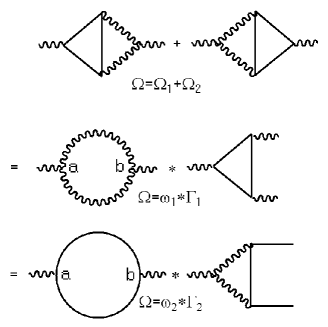
Figure 1: This sum $\Omega$ of two graphs $\Omega_{1},\Omega_{2}$ can be obtained in two different ways. We can either glue $\Gamma_{1}$ into $\omega_{1}$ by identifying the external edges of $\Gamma_{1}$ with the edges adjacent to the vertices $a$ or $b$ of $\omega_{1}$, or similarly, do so for the graphs $\omega_{2},\Gamma_{2}$, with the same result $\Omega$.

The short distance singularities of Feynman graphs then come solely from regions where all vertices are located at coinciding points. One has no problem to define the Feynman integrand in the configuration space of vertices at distinct locations, while a proper extension to diagonals is what is required [14, 15].

Due to the Hopf algebra structure of Feynman graphs we can define the renormalization of all such sectors without making recourse to any specific analytic properties of the expressions (Feynman integrals) representing those sectors. The only assumption we make is that in a sufficiently small neighborhood of such an ultralocal region (the neighborhood of a diagonal) we can define the scaling degree, –the powercounting–, in a sensible manner: combinatorics suffices. Analytic detail arising from quests for causality for example can be imposed later. This principle indeed goes far: almost all detail about the Feynman rules for propagators and vertices which goes beyond their scaling degree is unnecessary at this stage. Having determined these powercounting degrees and having chosen a renormalization scheme, we will soon formally define the principle of multiplicative subtraction which will tell us how we get local counterterms and finite renormalized quantities whatever the finer detail is of the Feynman rules. This is the strong combinatorial backbone of QFT, which ultimately has its source in the notion of a residue, and in the fundamental invariance properties of residues.

This is indeed a very useful application of the Hopf algebra: the decomposition into its primitives reveals the range over which the combinatorial structures of renormalization are stable to include, for example, fluctuations of the metric as long as the scaling degree of propagators is microlocally unchanged, as such fluctuation do not alter the residue of a bidegree one graph. This allows to understand the recent results of Brunetti and Fredenhagen [16] from a combinatorial viewpoint.

Its time now to define the Hopf algebra of Feynman graphs, which expresses this combinatorial backbone of renormalization theory.

1.2 Lie and Hopf algebras of Feynman graphs

We start giving some formal definitions. Our presentation follows [17].

First, we define $n$-particle irreducible ($n$-PI) graphs. We will exclude graphs with self-loops: no edge connects a vertex to itself. But we will allow for two different vertices to be connected by several edges. Note that self-loops are naturally excluded in a massless theory.

Definition 1

A $n$-particle irreducible graph ($n$-PI graph) $\Gamma$ consists of edges and vertices, without self-loops, such that upon removal of any set of $n$ of its edges it is still connected. Its set of edges is denoted by $\Gamma^{[1]}$ and its set of vertices is denoted by $\Gamma^{[0]}$. Edges and vertices can be of various different types.

The type of an edge is often indicate by the way we draw it: (un-)oriented straight lines, curly lines, dashed lines and so on. These types of edges, often called propagators in physicists parlance, are chosen with reference to Lorentz covariant wave equations: the propagator as the analytic expression assigned to an edge is an inverse wave operator with boundary conditions typically chosen in accordance with causality. We can, if desired, ignore such consideration by the choice of an Euclidean metric.

The types of vertices are determined by the types of edges to which they are attached:

Definition 2

For any vertex $v$ $\in\Gamma^{[0]}$ we call the set $f_{v}:=\{f\in\Gamma^{[1]}\mid v\cap f\not=\emptyset\}$ its type.

Note that $f_{v}$ is a set of edges.

Of particular importance are the 1PI graphs. They do not decompose into disjoint graphs upon removal of an edge. Note that any $n$-PI graphs is also $(n-1)$-PI, $\forall n\geq 2$. A graph which is not 1-PI is called reducible. Also, any connected graph is considered as 0-PI.

A further notion needed is the one of external and internal edges, introduced before.

Definition 3

An edge $f$ $\in\Gamma^{[1]}$ is internal, if $\{v_{f}\}:=f\cap\Gamma^{[0]}$ is a set of two elements.

So, internal edges connect two vertices of the graph $\Gamma$.

Definition 4

An edge $f$ $\in\Gamma^{[1]}$ is external, if $f\cap\Gamma^{[0]}$ is a set of one element.

As we exclude self-loops, this means that an external edge has an open end. Thus external edges are associated with a single vertex of the graph. These edges correspond to external particles interacting in the way prescribed by the graph.

We now turn to the possibilities of inserting graphs into each other. Our first requirement is to establish bijections between sets of edges so that we can define gluing operations.

Definition 5

We call two sets of edges $I_{1},I_{2}$ compatible, $I_{1}\sim I_{2}$, iff they contain the same number of edges, of the same type.

Definition 6

Two vertices $v_{1},v_{2}$ are of the same type, if $f_{v_{1}}$ is compatible with $f_{v_{2}}$.

Quite often, we will shrink a graph to a point. The only useful information still available after that process is about its set of external edges:

Definition 7

We define ${\bf res}(\Gamma)$ to be the result of identifying $\Gamma^{[0]}\cup\Gamma^{[1]}_{\rm int}$ with a point in $\Gamma$.

An example is

$$\;\raisebox{-7.11317pt}{\epsfbox{res.eps}}\;.$$

Note that ${\bf res}(\Gamma)^{[1]}\equiv{\bf res}(\Gamma)^{[1]}_{\rm ext}\sim\Gamma^{[1]}_{\rm ext}$. By construction all graphs which have compatibe sets of external edges have the same residue.

If the set $\Gamma^{[1]}_{\rm ext}$ is empty, we call $\Gamma$ a vacuumgraph, if it contains a single element we call the graph a tadpole graph. Vacuum graphs and tadpole graphs will be discarded in what follows. If $\Gamma^{[1]}_{\rm ext}$ contains two elements, we call $\Gamma$ a self-energy graph, if it contains more than two elements, we call it an interaction or vertex graph. Further we restrict ourselves to graphs which have vertices such that the cardinality of their types is $\geq 2$. In the presence of external fields, this can be relaxed.

At this stage, we are provided with a list of edges and vertices obtained typically, but not necessarily, from some QFT Lagrangian. Weights assigned to these elements allow to discriminate graphs formed from these objects by the means of powercounting. We can thus meaningfully speak about 1PI graphs which are superficially divergent or convergent - graphs $\Gamma$ such that the integral Eq.(1) attached to $\Gamma$ diverges or converges at the upper boundary of the final $r=\sum_{e\in\Gamma^{[1]}_{\rm int}}|k_{e}|$ integration in Eq.(2).

We are after a mechanism which eliminates all possible divergences coming from subintegrations. These can be detected by powercounting on the 1PI subgraphs, and we will soon introduce a Hopf algebra structure based on superficially divergent 1PI graphs.

1.3 External structures

Let us mention here one more useful notational device: the external structures of [3]. To each external edge $f\in\Gamma^{[1]}_{\rm ext}$ we assign an external momentum $p_{f}$, a vector in some (to be appropriately specified) vectorspace and impose the condition $\sum_{f\in\Gamma_{\rm ext}^{[1]}}p_{f}=0$. We let $E_{{\bf res}(\Gamma)}$ be the linear space of functions of those variables $p_{f}$ fulfilling this condition.

Following [3] we use a notation familiar from distribution theory to describe the evaluation of a graph $\Gamma$ by some Feynman rules $\phi:{\cal H}\to E_{{\bf res}(\Gamma)}$: with $\phi(\Gamma)\in E_{{\bf res}(\Gamma)}$, we denote by $\langle\sigma,\phi(\Gamma)\rangle$ the evaluation of $\phi(\Gamma)$ with respect to the distribution $\sigma$ on $E_{{\bf res}(\Gamma)}$, in the same way as $\langle\delta_{a},f\rangle=f(a)$ defines the evaluation of a function at $a$ by the pairing with a Dirac $\delta$-distribution supported at $a$.

A graph $\Gamma$ together with a distribution $\sigma$ we call a specified graph, and write $(\Gamma,\sigma)$ for such a pair. We can regard it as a graph with a further prescription how to evaluate it.

We will need these notions to keep track of our perturbative expansion: let us assume that the Lagrangian $L$ which is the source for our perturbative expansion is a sum over $k$ field monomials. Assume that $L$ contains $n$ different fields $\phi_{1},\ldots\phi_{n}$. Then to each monomial $P(\{\phi_{i}\})$ in $L$ we can assign the sequence $(i_{1},\ldots,i_{n})_{P}$, which tells us the degree of $P$ in each field. We call this sequence the field degree of $P$. If two monomials $P,P^{\prime}$ deliver equal field degrees, they both can be described by graphs with an equal residue in the above sense: their corresponding Feynman graphs $\Gamma$ will have identical external legs, hence identical residues ${\bf res}(\Gamma)$. Counterterms for such monomials are then calculated by suitable projections in $E_{{\bf res}(\Gamma)}$, implemented by distributions $\sigma_{P},\sigma_{P^{\prime}}$.

A typical example are the mass and wave function renormalization of a scalar propagator, with monomials $P=-m^{2}\phi^{2}/2$ and $P^{\prime}=\partial_{\mu}\phi\partial^{\mu}\phi/2$, say. Both monomials are quadratic in a scalar field $\phi$ and the contributions of two-point graphs to $P,P^{\prime}$ are obtained from

$$\langle\sigma_{P},\phi(\Gamma)\rangle$$

and

$$\langle\sigma_{P^{\prime}},\phi(\Gamma)\rangle,$$

with $\langle\sigma_{P},f(m^{2},q^{2})\rangle=\partial_{m^{2}}f\mid_{m^{2}=q^{2}}$ and $\langle\sigma_{P^{\prime}},f(m^{2},q^{2})\rangle=\partial_{q^{2}}f\mid_{m^{2}=q^{2}}$, for any function $f(m^{2},q^{2})$. Similarly, one extends to other cases for monomials of equal field degree, and one can conveniently express the formfactor decomposition of Green functions in this language.

In such a notation, all field monomials $P$ in the Lagrangian correspond to expressions $\langle\sigma_{P},\phi({\bf res}(\Gamma))\rangle$, where $\Gamma$ is a graph which external legs in accordance with the field degree of $P$, and one always has that

$$\langle\sigma_{P},\phi(\Gamma)\rangle=\rho_{P}(\Gamma)\langle\sigma_{P},\phi({\bf res}(\Gamma))\rangle,$$ (12)

where $\rho_{P}(\Gamma)$ is a scalar function (the form-factor) which fulfills that on disjoint diagrams $\rho_{P}(\Gamma_{1}\Gamma_{2})\equiv\rho_{P}(\Gamma_{2}\Gamma_{1})=\rho_{P}(\Gamma_{1})\rho_{P}(\Gamma_{2})$, $\forall P$, regardless of the fact that $\langle\sigma_{P},\phi(\Gamma_{P})\rangle$ can be matrix-valued. The simple fact that the action is a Lorentz scalar indeed mandates that a formfactor decomposition into scalar coefficients is always possible, and is in accordance with the product structure of graphs: the evaluation of a product is the commutative product of the evaluations.

It is those scalar coefficients which appear as characters on the Hopf algebra of graphs which we describe below. Our route will be to first define a pre-Lie product on graphs, which at the same time establishes a Lie bracket upon its antisymmetrization, and then take the dual of the universal enveloping algebra of the so-obtained Lie algebra as the Hopf algebra under consideration. This indeed provides the always commutative Hopf algebra which underlies the disentanglement of graphs into their divergent parts, the combinatorial backbone of local quantum field theory.

1.4 The Pre-Lie Structure

Consider two graphs $\Gamma_{1},\Gamma_{2}$. Assume that $\Gamma_{2}$ is an interaction graph. For a chosen vertex $v_{i}\in\Gamma_{1}^{[0]}$ such that $f_{v_{i}}\sim\Gamma^{[1]}_{2,\rm ext}$, we define

$$\Gamma_{1}\star_{v_{i}}\Gamma_{2}=\Gamma_{1}/v_{i}\cup\Gamma_{2}/\Gamma^{[1]}_{2,\rm ext},$$ (13)

where in the union of these two sets we create a new graph such that for every edge $f_{j}\in f_{v_{i}}$, $\{v_{f_{j}}\}$ contains precisely one element in $\Gamma_{2}^{[0]}$. Then we sum over all possible bijection between $f_{vi}$ and $\Gamma_{2,\rm ext}^{1}$, and normalize such that topologically different graphs are generated precisely once.

We now define

$$\Gamma_{1}\star\Gamma_{2}=\sum_{w\in\Gamma_{1}^{[0]}\atop f_{w}\sim\Gamma^{[1]}_{2,\rm ext}}\Gamma_{1}\star_{w}\Gamma_{2}.$$ (14)

All this can be easily generalized to the insertion of self-energy graphs, replacing internal edges by self-energy graphs which have the corresponding external edges.

We also define the insertion of specified graphs in the similar vein, by requiring that

$$(\Gamma_{1},\sigma_{1})\star(\Gamma_{2},\sigma_{2})=(\Gamma_{1}\star\Gamma_{2},\sigma_{1}).$$ (15)

That is, by inserting a graph, we forget about conditions imposed on its external legs. Dually, for the Hopf algebra below, this corresponds to the fact that upon disentangling a graph, we have the freedom to impose constraints -renormalization conditions- to its subgraphs.

Proposition 8

The operation $\star$ is pre-Lie:

$$[(\Gamma_{1},\sigma_{1})\star(\Gamma_{2},\sigma_{2})]\star(\Gamma_{3},\sigma_{3}) - (\Gamma_{1},\sigma_{1})\star[(\Gamma_{2},\sigma_{2})\star(\Gamma_{3},\sigma_{3})]$$

$$=[(\Gamma_{1},\sigma_{1})\star(\Gamma_{3},\sigma_{3})]\star(\Gamma_{2},\sigma_{2}) - (\Gamma_{1},\sigma_{1})\star[(\Gamma_{3},\sigma_{3})\star(\Gamma_{2},\sigma_{2})].$$

To sketch the proof, which is elementary for unspecified graphs, we note that the insertion of subgraphs is a local operation, and that on both sides, the difference amounts to plugging the subgraphs $\Gamma_{2},\Gamma_{3}$ into $\Gamma_{1}$ at disjoint places, which is evidently symmetric under the exchange of $\Gamma_{2}$ with $\Gamma_{3}$. For specified graphs, we choose a color for each evaluation $\sigma_{i}$ under consideration, and represent the pair $(\sigma,\Gamma)$ by a colored graph. Coloring does not spoil the locality of the insertions.

If needed, this can be generalized in a way as to maintain constraints on external legs when inserting a graph into another, still maintaining the pre-Lie structure. Integration over the edges according to Eq.(1) is then done in a way such that it obeys the constraints valid for each subgraph. Such extensions are useful in practice when one desires to decompose graphs into various analytic subfactors [18], and underly the decomposition into primitives discussed in section five.

In most of what follows we only use unspecified graphs, with the generalization to specified graphs being evident.

We get a Lie algebra ${\cal L}$ by antisymmetrizing this operation,

$$[\Gamma_{1},\Gamma_{2}]=\Gamma_{1}\star\Gamma_{2}-\Gamma_{2}\star\Gamma_{1}$$ (16)

and a Hopf algebra ${\cal H}$ as the dual of the universal enveloping algebra of this Lie algebra. Typically, one restricts attention to graphs which are superficially divergent, with residues corresponding to field monomials in the Lagrangian.

Superficially convergent graphs can be incorporated using the trivial abelian Lie algebra which they span when one regards them as specified graphs. The fact that they do not contribute to counterterms in the Lagrangian means that they are annihilated by external structures which project onto the contributions to superficially divergent field monomials $P$. Hence they have a vanishing Lie bracket among themselves and furthermore form a semi-direct product with their superficially divergent cousins [3]. An example of the Lie bracket Eq.(16) is provided by Fig.(2).

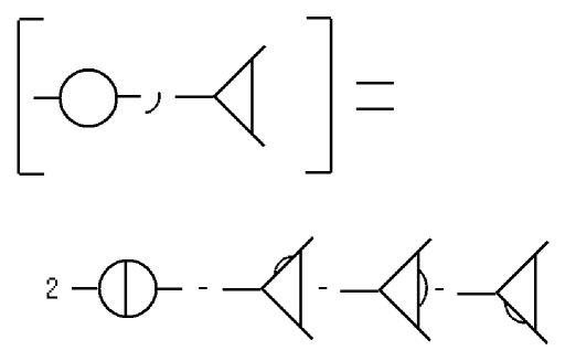
Figure 2: The Lie-bracket $[\Gamma_{1},\Gamma_{2}]=\Gamma_{1}\star\Gamma_{2}-\Gamma_{2}\star\Gamma_{1}$.

1.5 The principle of multiplicative subtraction

Having defined Lie algebra structures on graphs, it is now easy to harvest them to give a clear conceptual meaning to the renormalization process. As announced, we just have to dualize the universal enveloping algebra ${\cal U(L)}$ of ${\cal L}$ and obtain a commutative, but not cocommutative Hopf algebra ${\cal H}$ [3].

From now on, when we want to distinguish carefully between the Hopf and Lie algebras of Feynman graphs we write $\delta_{\Gamma}$ for the multiplicative generators of the Hopf algebra and write $Z_{\Gamma}$ for the dual basis of the universal enveloping algebra of the Lie algebra ${\cal L}$ with pairing

$$\langle Z_{\Gamma},\delta_{\Gamma^{\prime}}\rangle=\delta^{K}_{\Gamma,\Gamma^{\prime}},$$ (17)

where on the rhs we have the Kronecker $\delta^{K}$, and extend the pairing by means of the coproduct

$$\langle Z_{\Gamma_{1}}Z_{\Gamma_{2}},X\rangle=\langle Z_{\Gamma_{1}}\otimes Z_{\Gamma_{2}},\Delta(X)\rangle.$$ (18)

Quite often, we want to refer to the graph(s) which index an element in ${\cal H}$ or ${\cal L}$. For that purpose, for each element in ${\cal H}$ and each element in ${\cal L}$ we introduce a map to graphs:

$$\overline{Z_{X}}=X,\overline{\delta_{X}}=X.$$ (19)

As we already have emphasized the Hopf algebra of rooted trees is the role model for the Hopf algebras of Feynman graphs which underly the process of renormalization when formulated perturbatively at the level of Feynman graphs. The following formulas should be of no surprise for the reader acquainted with the universal Hopf algebra of rooted trees and are a straightforward generalization of similar formulas for rooted tree Hopf algebras [19].

First of all, we start considering one-particle irreducible graphs as the linear generators of the Hopf algebra, with their disjoint union as product. We then identify the Hopf algebra as described above by a coproduct $\Delta:{\cal H}\to{\cal H}\otimes{\cal H}$:

$$\Delta(\Gamma)=\Gamma\otimes 1+1\otimes\Gamma+\sum_{\gamma{\subset}\Gamma}\gamma\otimes\Gamma/\gamma,$$ (20)

where the sum is over all unions of one-particle irreducible (1PI) superficially divergent proper subgraphs and we extend this definition to products of graphs so that we get a bialgebra. The above sum should, when needed, also run over appropriate external structures to specify the appropriate type of local insertion [3] which appear in local counterterms, which we omitted in the above sum for simplicity. Fig.(3) gives an example of a coproduct.

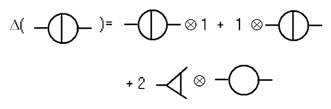
Figure 3: The coproduct $\Delta(\Gamma)$.

For any Hopf algebra element $X$ we often write a shorthand for its coproduct

$$\Delta(X)=\widetilde{\Delta}(X)+X\otimes 1+1\otimes X=X\otimes 1+1\otimes X+X^{\prime}\otimes X^{\prime\prime}.$$

Let now $X$ be a 1PI graph. For each term in the sum $\widetilde{\Delta}(X)=\sum_{i}X^{\prime}\otimes X^{\prime\prime}$ we have unique gluing data $G_{i}$ such that

$$X=X^{\prime\prime}\star_{G_{i}}X^{\prime},\;\forall i.$$ (21)

These gluing date describe the necessary bijections to glue the components $X^{\prime}$ back into $X^{\prime\prime}$ so as to obtain $X$.

The counit $\bar{e}$ vanishes on any non-trivial Hopf algebra element, $\bar{e}(1)=1,\,\bar{e}(X)=0$. At this stage we have a commutative, but typically not cocommutative bialgebra. It actually is a Hopf algebra as the antipode in such circumstances comes for free as

$$S(\Gamma)=-\Gamma-\sum_{\gamma{\subset}\Gamma}S(\gamma)\Gamma/\gamma.$$ (22)

The next thing we need are Feynman rules, which we regard as maps $\phi:{\cal H}\to V$ from the Hopf algebra of graphs ${\cal H}$ into an appropriate space $V$.

Over the years, physicists have invented many calculational schemes in perturbative quantum field theory, and hence it is of no surprise that there are many choices for this space.

For example, if we want to work on the level of Feynman integrands in a BPHZ scheme, we could take as this space a suitable space of Feynman integrands (realized either in momentum space or configuration space, whatever suits). An alternative scheme would be the study of regularized Feynman integrals, for example the use of dimensional regularization would assign to each graph a Laurent-series with poles of finite order in a variable $\varepsilon$ near $\varepsilon=0$, and we would obtain characters evaluating in this ring, an approach leading to the Riemann-Hilbert decomposition described below. In any case, we will have $\phi(\Gamma_{1}\Gamma_{2})\equiv\phi(\Gamma_{2}\Gamma_{1})=\phi(\Gamma_{1})\phi(\Gamma_{2})$, $\forall\phi:{\cal H}\to V$.

Then, with the Feynman rules providing a canonical character $\phi$, we will have to make one further choice: a renormalization scheme. This is is a map $R:V\to V$, and we demand that is does not modify the UV-singular structure: in BPHZ language, it should not modify the Taylor expansion of the integrand for the first couple of terms divergent by powercounting. In dimensional regularization, then, we demand that it does not modify the pole terms in $\varepsilon$. Furthermore, we require it to make the pair $(V,R)$ into a Baxter algebra, as in Eq.(6).

Finally, the principle of multiplicative subtraction emerges: we define a further character $S_{R}^{\phi}$ which deforms $\phi\circ S$ slightly and delivers the counterterm for $\Gamma$ in the renormalization scheme $R$:

$$S_{R}^{\phi}(\Gamma)=-R[\phi(\Gamma)]-R\left[\sum_{\gamma{\subset}\Gamma}S_{R}^{\phi}(\gamma)\phi(\Gamma/\gamma)\right]$$ (23)

which should be compared with the undeformed

$$\phi\circ S=-\phi(\Gamma)-\sum_{\gamma{\subset}\Gamma}\phi\circ S(\gamma)\phi(\Gamma/\gamma).$$ (24)

Then, the classical results of renormalization theory follow immediately [9, 12, 19]. We obtain the renormalization of $\Gamma$ by the application of a renormalized character

$$\Gamma\to S_{R}^{\phi}\star\phi(\Gamma)$$

and the $\bar{R}$ operation as

$$\bar{R}(\Gamma)=\phi(\Gamma)+\sum_{\gamma{\subset}\Gamma}S_{R}^{\phi}(\gamma)\phi(\Gamma/\gamma),$$ (25)

so that we have

$$S_{R}^{\phi}\star\phi(\Gamma)=\bar{R}(\Gamma)+S_{R}^{\phi}(\Gamma).$$ (26)

In the above, we have given all formulas in their recursive form. Zimmermann’s original forest formula solving this recursion is obtained when we trace our considerations back to the fact that the coproduct of rooted trees can be written in non-recursive form, and similarly the antipode [12]. We will come back below to this transition between graphs and trees. Also, we note that the principle of multiplicative subtraction can be formulated in much larger generality, as it is a basic combinatorial principle, see for example [20] for another appearance of this principle.

1.6 The Bidegree

A fundamental notion is the bidegree of a 1PI graph (see [21] for a convenient review of notions needed here). Usually, induction in perturbative QFT, aiming to prove a desired result is carried out using induction over the loop number, an obvious grading for 1PI graphs. On quite general grounds, for our Hopf algebras there exists another grading, which is actually much more useful. We call it the bidegree, ${\rm bid}(\Gamma)$. To motivate it, consider a superficially divergent $n$-loop graph $\Gamma$ which has no divergent subgraph. It is evident that its short-distance singularities can be treated by a single subtraction, for any $n$. It is not the loop number, but the number of divergent subgraphs which is the most crucial notion here. Fortunately, this notion has a precise meaning in the Hopf algebra of superficially divergent graphs using the projection into the augmentation ideal. This indeed counts the degree in renormalization parts of a graph: an overall superficially convergent graph has bidegree zero by definition, a primitive Hopf algebra element has bidegree one, and so on.

So we have ${\cal H}=\bigoplus_{i=0}^{\infty}{\cal H}^{(i)}$, with ${\rm bid}({\cal H}^{(i)})=i$. To define this decomposition, let ${\cal H}_{\rm Aug}$ be the augmentation ideal of the Hopf algebra, and let $P:{\cal H}\to{\cal H}_{\rm Aug}$ be the corresponding projection $P={\rm id}-E\circ\bar{e}$, with $E(q)=qe$. Let $\widetilde{\Delta}(X)=\Delta(X)-e\otimes X-X\otimes e$, as before. $\widetilde{\Delta}$ is still coassociative, and for any $X\in{\cal H}_{\rm Aug}$ there exists a unique maximal $k$ such that $\widetilde{\Delta}^{k-1}(X)\in[{\cal H}^{(1)}]^{\otimes k}.$ Here, ${\cal H}^{(1)}$ is the linear span of primitive elements $z$: $\Delta(z)=z\otimes e+e\otimes z$.

Definition 9

The map $X\to k$ obtained as described above is called the bidegree $deg_{p}$ of $X$.

The bidegree is conserved under the coproduct and under the product (disjoint union). Typically, all properties connected to questions of renormalization theory can be proven more efficiently using the grading by the bidegree instead of the loop number. In particular, we will discuss below the interplay between Hochschild cohomology and the bidegree, which explains locality of counterterms and finiteness of renormalized graphs rather succinctly. But let us first come to an even more succinct formulation of renormalization theory, making use of the existence of complex regularizations.

2 Renormalization and the Riemann–Hilbert
problem

2.1 The Birkhoff decomposition

The Feynman rules in dimensional or analytic regularization determine a character $\phi$ on the Hopf algebra which evaluates as a Laurent series in a complex regularization parameter $\varepsilon$, with poles of finite order, this order being bounded by the bidegree of the Hopf algebra element to which $\phi$ is applied. In minimal subtraction, $\phi_{-}:=S^{\phi}_{R=MS}$ has similar properties: it is a character on the Hopf algebra which evaluates as a Laurent series in a complex regularization parameter $\varepsilon$, with poles of finite order, this order being bounded by the bidegree of the Hopf algebra element to which $S^{\phi}_{R=MS}$ is applied, only that there will be no powers of $\varepsilon$ which are $\geq 0$. Then, $\phi_{+}:=S^{\phi}_{R=MS}\star\phi$ is a character which evaluates in a Taylor series in $\varepsilon$, all poles are eliminated. We have the Birkhoff decomposition

$$\phi=\phi_{-}^{-1}\star\phi_{+}.$$ (27)

This establishes an amazing connection between the Riemann–Hilbert problem and renormalization [3, 4]. It uses in a crucial manner once more that the multiplicativity constraints Eq.(6),

$$R[xy]+R[x]R[y]=R[R[x]y]+R[xR[y]],$$

ensure that the corresponding counterterm map $S_{R}$ is a character as well,

$$S_{R}[xy]=S_{R}[x]S_{R}[y],\;\forall x,y\in H,$$ (28)

by making the target space of the Feynman rules into a Baxter algebra, characterized by this multiplicativity constraint. The connection between Baxter algebras and the Riemann–Hilbert problem, which lurks in the background here, remains largely unexplored, as of today.

Renormalization in the MS scheme can now be summarized in one sentence: with the character $\phi$ given by the Feynman rules in a suitable regularization scheme and well-defined on any small curve around $\varepsilon=0$, find the Birkhoff decomposition $\phi_{+}(\varepsilon)=\phi_{-}\star\phi$.

The unrenormalized analytic expression for a graph $\Gamma$ is then $\phi[\Gamma](\varepsilon)$, the MS-counterterm is $S_{{MS}}(\Gamma)\equiv\phi_{-}[\Gamma](\varepsilon)$ and the renormalized expression is the evaluation $\phi_{+}[\Gamma](0)$. Once more, note that the whole Hopf algebra structure of Feynman graphs is present in this group: the group law demands the application of the coproduct, $\phi_{+}=\phi_{-}\star\phi\equiv S_{MS}^{\phi}\star\phi$.

But still, one might wonder what a huge group this group of characters really is. What one confronts in QFT is the group of diffeomorphisms of physical parameter: low and behold, changes of scales and renormalization schemes are just such (formal) diffeomorphisms. So, for the case of a massless theory with one coupling constant $g$, for example, this just boils down to formal diffeomorphisms of the form

$$g\to\psi(g)=g+c_{2}g^{2}+\ldots.$$

The group of one-dimensional diffeomorphisms of this form looks much more manageable than the group of characters of the Hopf algebras of Feynman graphs of such a theory.

2.2 Diffeomorphisms of physical parameters

Thus, it would be very nice if the whole Birkhoff decomposition could be obtained at the level of diffeomorphisms of the coupling constants. The crucial ingredient is to realize the role of a standard QFT formula of the form

$$g_{\rm new}=g_{\rm old}\;Z_{1}Z_{2}^{-3/2},$$ (29)

which expresses how to obtain the new coupling in terms of a diffeomorphism of the old. This was achieved in [4], recognizing this formula as a Hopf algebra homomorphism from the Hopf algebra of diffeomorphism to the Hopf algebra of Feynman graphs, regarding $Z_{g}=Z_{1}/Z_{2}^{3/2}$, a series over counterterms for all 0PI graphs with the external leg structure corresponding to the coupling $g$, in two different ways. It is at the same time a formal diffeomorphism in the coupling constant $g_{\rm old}$ and a formal series in Feynman graphs. As a consequence, there are two competing coproducts acting on $Z_{g}$. That both give the same result defines the required homomorphism, which transposes to a homomorphism from the largely unknown group of characters of ${\cal H}$ to the one-dimensional diffeomorphisms of this coupling.

The crucial fact in this is the recognition of the Hopf algebra structure of diffeomorphisms by Connes and Moscovici [22]: Assume you have formal diffeomorphisms $\phi,\psi$ in a single variable

$$x\to\phi(x)=x+\sum_{k>1}c_{k}^{\phi}x^{k},$$ (30)

and similarly for $\psi$. How do you compute the Taylor coefficients $c^{\phi\circ\psi}_{k}$ for the composition $\phi\circ\psi$ from the knowledge of the Taylor coefficients $c_{k}^{\phi},c_{k}^{\psi}$? It turns out that it is best to consider the Taylor coefficients

$$\delta_{k}^{\phi}=\log(\phi^{\prime}(x))^{(k)}(0)$$ (31)

instead, which are as good to recover $\phi$ as the usual Taylor coefficients. The answer lies then in a Hopf algebra structure:

$$\delta^{\phi\circ\psi}_{k}=m\circ(\tilde{\psi}\otimes\tilde{\phi})\circ\Delta_{CM}(\delta_{k}),$$ (32)

where $\tilde{\phi},\tilde{\psi}$ are characters on a certain Hopf algebra ${\cal H}_{CM}$ (with coproduct $\Delta_{CM}$) so that $\tilde{\phi}(\delta_{i})$ $=$ $\delta_{i}^{\phi}$, and similarly for $\tilde{\psi}$. Thus one finds a Hopf algebra with abstract generators $\delta_{n}$ such that it introduces a convolution product on characters evaluating to the Taylor coefficients $\delta_{n}^{\phi},\delta_{n}^{\psi}$, such that the natural group structure of these characters agrees with the diffeomorphism group.

It turns out that this Hopf algebra of Connes and Moscovici is intimately related to rooted trees in its own right [19], signalled by the fact that it is linear in generators on the rhs, as are the coproducts of rooted trees and graphs.

There are a couple of basic facts which enable to make in general the transition from this rather foreign territory of the abstract group of characters of a Hopf algebra of Feynman graphs (which, by the way, equals the Lie group assigned to the Lie algebra with universal enveloping algebra the dual of this Hopf algebra) to the rather concrete group of diffeomorphisms of physical observables. These steps are

• Recognize that $Z$ factors are given as counterterms over formal series of graphs starting with 1, graded by powers of the coupling, hence invertible.

• Recognize the series $Z_{g}$ as a formal diffeomorphism, with Hopf algebra coefficients.

• Establish that the two competing Hopf algebra structures of diffeomorphisms and graphs are consistent in the sense of a Hopf algebra homomorphism.

• Show that this homomorphism transposes to a Lie algebra and hence Lie group homomorphism.

This works out extremely nicely, with details given in [4]. In particular, the effective coupling $g_{\rm eff}(\varepsilon)$ now allows for a Birkhoff decomposition in the space of formal diffeomorphisms

$$g_{\rm eff}(\varepsilon)=g_{\rm eff-}(\varepsilon)^{-1}\circ g_{\rm eff+}(\varepsilon)$$ (33)

where $g_{\rm eff-}(\varepsilon)$ is the bare coupling and $g_{\rm eff+}(0)$ the renormalized effective coupling while the coupling can be regarded as the coupling in any theory which has a single interaction term. If there are multiple interaction terms in the Lagrangian, one finds similar results relating the group of characters of the corresponding Hopf algebra to the group of formal diffeomorphisms in the multidimensional space of coupling constants.

There are some false but pertinent claims in the literature with regards to the extension of this result to massless QED and other theories with spin [23]. The above results hold as they stand for massless QED, with the relevant Hopf algebra homomorphism given by $e_{\rm new}=Z_{3}^{-1/2}e_{\rm old}$.

The confusion arises from the assumption that in theories with spin, the noncommutativity of Green functions demands the use of a noncommutative noncocommutative Hopf algebra, ignoring the commutative Hopf algebra obtained from the pre-Lie algebra of graphs insertions above. This is patently wrong and ignores the fact that the relevant characters on the Hopf algebra are given by the coefficient functions of the tree-level form factors, and these coefficient functions are scalar characters

$$\rho(\Gamma_{1}\Gamma_{2})=\rho(\Gamma_{2}\Gamma_{1})=\rho(\Gamma_{1})\rho(\Gamma_{2}),$$ (34)

on a commutative Hopf algebra, with all noncommutativity residing in the matrix structures multiplying those form-factors. A typical such character $\rho$ is provided by the Feynman rules $\phi$ of massless QED applied to a fermion self-energy graph $\Gamma$ with external momentum $p\!\!\!/$ say, where we have

$$\phi(\Gamma)=\rho(\Gamma)p\!\!\!/,$$ (35)

with $\rho(\Gamma)=Tr(p\!\!\!/\phi(\Gamma))/p^{2}$, and $p\!\!\!/=\phi({\bf res}(\Gamma))$, and indeed, the matrix structure of $p\!\!\!/$ plays no further role with respect to the commutativity of ${\cal H}$.

3 Multiple rescalings

So we have singled out $MS$ as a special character, providing us with a Birkhoff decomposition. So what about other renormalization schemes: are they less meaningful? Not quite.

Let us come back to unrenormalized Feynman graphs, and their evaluation by some chosen character $\phi$, and let us also choose a renormalization scheme $R$. The group structure of such characters on the Hopf algebra can be used in an obvious manner to describe the change of renormalization schemes. This has very much the structure of a generalization of Chen’s Lemma [6].

3.1 Chen’s Lemma

Consider $S_{R}\star\phi$. Let us change the renormalization scheme from $R$ to $R^{\prime}$. How is the renormalized character $S_{R^{\prime}}\star\phi$ related to the renormalized character $S_{R}\star\phi$? The answer lies in the group structure of characters:

$$S_{R^{\prime}}\star\phi=[S_{R^{\prime}}\star S_{R}\circ S]\star[S_{R}\star\phi],$$ (36)

which generalizes Chen’s Lemma on iterated integrals [6]. We inserted a unit $\eta$ with respect to the $\star$-product in form of $\eta=S_{R}\circ S\star S_{R}\equiv S_{R}^{-1}\star S_{R}$, and can now read the rerenormalization, switching between the two renormalization schemes, as composition with the renormalized character $S_{R^{\prime}}\star S_{R}^{-1}$. Note that $S_{R^{\prime}}\star S_{R}\circ S$ is a renormalized character indeed: if $R,R^{\prime}$ are both self-maps of $V$ which do not alter the short-distance singularities as discussed before, then in the ratio $S_{R^{\prime}}\star S_{R}\circ S$ those singularities drop out.

Similar considerations apply to a change of scales which determine a character [6]. If $\mu$ is a dimensionful parameter which dominates the process under consideration and which appears in a character $\phi=\phi(\mu)$, then the transition $\mu\to\mu^{\prime}$ is implemented in the group by acting on the right with the renormalized character $\psi_{\mu,\mu^{\prime}}^{\phi}:=\phi(\mu)\circ S\star\phi(\mu^{\prime})$ on $\phi(\mu)$,

$$\phi(\mu^{\prime})=\phi(\mu)\star\psi_{\mu,\mu^{\prime}}^{\phi}.$$ (37)

Let us note that this Hopf algebra structure can be efficiently automated as an algorithm for practical calculations exhibiting the full power of this combinatorics [24].

Now, assume we compute Feynman graphs by some Feynman rules in a given theory and decide to subtract UV singularities at a chosen renormalization point $\mu$. This amounts, in our language, to saying that the map $S_{R}$ is parametrized by this renormalization point: $S_{R}=S_{R_{\mu}}$. Typically, one has for $R_{\mu}:V\to V$,

$$R_{\mu}(ab)=R_{\mu}(a)\,R_{\mu}(b),$$ (38)

in accordance with but stronger than the multiplicativity constraints.

Then, let $\Phi(\mu,\mu^{\prime})$ be the ratio $\Phi(\mu,\mu^{\prime})=S_{R_{\mu}}\star\phi(\mu^{\prime})$. We then have the groupoid law as part of the before-mentioned Chen’s lemma [6, 7]

$$\Phi(\mu,\eta)\star\Phi(\eta,\mu^{\prime})=\Phi(\mu,\mu^{\prime}),$$ (39)

thanks to Eq.(38).

3.2 Automorphisms of ${\cal H}$

We further note that the use of external structures always allows to pullback renormalization schemes to automorphisms of the Hopf algebra by solving the equation

$$S_{R}^{\phi}\circ S=\phi\circ\Theta_{R},$$ (40)

for the automorphism $\Theta_{R}:{\cal H}\to{\cal H}$. Starting from primitive elements $\Gamma$, this can be solved to determine appropriate external structures, following the guidance of [6], solving by a recursion over the bidegree.

The full group structure of the group of characters of the Hopf algebra has barely been used in practice yet, with some notable exceptions in [24, 25], but it provides an enormously rich set of new tools for the investigation of QFT. One striking aspect is that it allows insight into the hardest problem of QFT: understanding the analytic aspects of the perturbative expansion, by laying bare the way in which analytic input enters the combinatorics of renormalization, and by allowing nonperturbative results completely based on the Hopf and Lie algebra structures, for example the beautiful duality between the scaling variable and the coupling discovered in [26].

Harvesting the combinatorial structure of QFT emphasizes the crucial role played by bidegree one graphs and their residues. Relations between such diagrams are often consequences of symmetries in the Lagrangian -BRST symmetry after the quantization of a local gauge symmetry, supersymmetry, or both. Even more striking though are relations which can not be traced back to such an origin. Typically they come as analytic surprises after the calculation of different diagrams. To get an idea of an underlying conceptual source for such relations, we have to look at our main theme, insertion and elimination of subgraphs, more closely.

4 Derivations on the Hopf algebra

Having defined the Hopf- and Lie algebras of Feynman graphs, it is profitable to look into representations of the Lie algebra as derivations on the Hopf algebra, following [17].

4.1 Representations of ${\cal L}$

The Lie algebra ${\cal L}$ gives rise to two representations acting as derivations on the Hopf algebra ${\cal H}$:

$$Z^{+}_{\Gamma}\times\delta_{X}=\delta_{X\star\Gamma}$$ (41)

and

$$Z^{-}_{\Gamma}\times\delta_{X}=\sum_{i}\langle Z^{+}_{\Gamma},\delta_{X^{\prime}_{(i)}}\rangle\delta_{{X^{\prime\prime}_{(i)}}}.$$ (42)

Furthermore, we stress again that any term in the coproduct of a 1PI graph $\Gamma$ determines gluing data $G_{i}$ such that

$$\Gamma=\Gamma^{\prime\prime}_{(i)}\star_{G_{i}}\Gamma^{\prime}_{(i)},\forall i.$$

Here, $G_{i}$ specifies vertices in $\Gamma^{\prime\prime}_{(i)}$ and bijections of their types with the elements of $\Gamma^{\prime}_{(i)}$ such that $\Gamma$ is regained from its parts:

$$\;\raisebox{-7.11317pt}{\epsfbox{pica.eps}}\;.$$

The first line gives a term $(i)$ in the coproduct, decomposing this graph into its only divergent subgraph (assuming we have chosen $\phi^{3}$ in six dimensions, say) and the corresponding cograph, the second line shows the gluing $G_{i}$ for this term, in this example.

We want to understand the commutator

$$[Z_{\Gamma_{1}}^{+},Z_{\Gamma_{2}}^{-}],$$ (43)

acting as a derivation on the Hopf algebra element $\delta_{X}$. To this end introduce

$$Z_{[\Gamma_{1},\Gamma_{2}]}\times\delta_{X}=\sum_{i}\langle Z_{\Gamma_{2}}^{+},\delta_{X^{\prime}_{(i)}}\rangle\delta_{X^{\prime\prime}_{(i)}\star_{G_{i}}\Gamma_{1}}.$$ (44)

Here, the gluing operation $G_{i}$ still acts such that each topologically different graph is generated with unit multiplicity:

$$\;\raisebox{-7.11317pt}{\epsfbox{picb.eps}}\;.$$

4.2 Insertion and Elimination

So finally we are free to exchange graphs, by eliminating one and inserting the other.

Theorem 10

[17]. For all 1PI graphs $\Gamma_{i}$, s.t. ${\bf res}(\Gamma_{1})={\bf res}(\Gamma_{2})$ and ${\bf res}(\Gamma_{3})={\bf res}(\Gamma_{4})$, the bracket

$$[Z_{[\Gamma_{1},\Gamma_{2}]},Z_{[\Gamma_{3},\Gamma_{4}]}] = +Z_{[\overline{Z_{[\Gamma_{1},\Gamma_{2}]}\times\delta_{\Gamma_{3}}},\Gamma_{4}]}-Z_{[\Gamma_{3},\overline{Z_{[\Gamma_{2},\Gamma_{1}]}\times\delta_{\Gamma_{4}}}]}$$

$$-Z_{[\overline{Z_{[\Gamma_{3},\Gamma_{4}]}\times\delta_{\Gamma_{1}}},\Gamma_{2}]}+Z_{[\Gamma_{1},\overline{Z_{[\Gamma_{4},\Gamma_{3}]}\times\delta_{\Gamma_{2}}}]}$$

$$-\delta^{K}_{\Gamma_{2},\Gamma_{3}}Z_{[\Gamma_{1},\Gamma_{4}]}+\delta^{K}_{\Gamma_{1},\Gamma_{4}}Z_{[\Gamma_{3},\Gamma_{2}]},$$

defines a Lie algebra of derivations acting on the Hopf algebra ${\cal H}$ via

$$Z_{[\Gamma_{i},\Gamma_{j}]}\times\delta_{X}=\sum_{I}\langle Z^{+}_{\Gamma_{2}},\delta_{X^{\prime}_{(i)}}\rangle\delta_{X^{\prime\prime}_{(i)}\star_{G_{i}}\Gamma_{1}},$$ (45)

where the gluing data $G_{i}$ are normalized as before.

The Kronecker $\delta^{K}$ terms just eliminate the overcounting when combining all cases in a single equation.

We note that $Z_{[\Gamma,\Gamma]}\times\delta_{X}=k_{\Gamma}\delta_{X}$, where $k_{\Gamma}$ is the number of appearances of $\Gamma$ in $X$ and where we say that a graph $\Gamma$ appears $k$ times in $X$ if $k$ is the largest integer such that

$$\langle\Gamma^{k}\otimes{\rm id},\Delta(\delta_{X})\rangle$$ (46)

is non-vanishing. Also $I:Z_{[\Gamma_{1},\Gamma_{2}]}\to Z_{[\Gamma_{2},\Gamma_{1}]}$ is an anti-involution such that

$$I([Z_{[\Gamma_{1},\Gamma_{2}]},Z_{[\Gamma_{3},\Gamma_{4}]}])=-[I(Z_{[\Gamma_{1},\Gamma_{2}]}),I(Z_{[\Gamma_{3},\Gamma_{4}]})].$$ (47)

Furthermore

$$[Z_{[\Gamma_{1},\Gamma_{2}]},Z_{[\Gamma_{2},\Gamma_{1}]}]=Z_{[\Gamma_{1},\Gamma_{1}]}-Z_{[\Gamma_{2},\Gamma_{2}]}.$$

By construction, we have

Proposition 11

$$Z^{+}_{\Gamma}\equiv Z_{[\Gamma,{\bf res}(\Gamma)]},$$

$$Z^{-}_{\Gamma}\equiv Z_{[{\bf res}(\Gamma),\Gamma]},$$

and $[Z^{-}_{X},Z^{-}_{Y}]=-Z^{-}_{\overline{[Z^{+}_{X},Z^{+}_{Y}]}}.$

Finally,

Proposition 12

$$[Z_{[\Gamma_{1},{\bf res}(\Gamma_{1})]},Z_{[{\bf res}(\Gamma_{2}),\Gamma_{2}]}] = \delta^{K}_{{\bf res}(\Gamma_{1}),{\bf res}(\Gamma_{2})}Z_{[\Gamma_{1},\Gamma_{2}]}+\delta^{K}_{\Gamma_{1},\Gamma_{2}}Z_{[{\bf res}(\Gamma_{2}),{\bf res}(\Gamma_{1})]}$$

$$-Z^{-}_{\overline{Z_{[{\bf res}(\Gamma_{1}),\Gamma_{1}]}\times\delta_{\Gamma_{2}}}}-Z^{+}_{\overline{Z_{[{\bf res}(\Gamma_{2}),\Gamma 2]}\times\delta_{\Gamma_{1}}}}.$$

These derivations provide a convenient mean to relate the insertion of subgraphs at different places to Galois symmetries in Feynman graphs, to be discussed below.

5 Primitivity

The letters in which QFT wants to be formulated are primitive 1PI graphs. But QFT speaks in manners more subtle than words: the letters do not come in linear order, but are inserted into each other in a highly structured way as we saw. How fluent are we in that language? Well, the combinatorial structures revealed so far allow us to decipher the content of QFT -the general Feynman graphs- completely in terms of these underlying letters. This features the residue as the central notion in quantum field theory, with each letter providing its own unique residue, a renormalization group invariant which connects the topology of the graph to number theory [18, 27, 28, 29, 30]. Let us discuss the disentanglement of Feynman graphs into these residues now.

Consider $\Gamma_{1}\star_{i}\Gamma_{2}$, for primitive graphs $\Gamma_{1},\Gamma_{2}$ and insertion at a compatible vertex $i$. Both graphs provide a first order pole, how do these two first order poles determine the second order pole in $\Gamma_{1}\star_{i}\Gamma_{2}$? And how are the higher order poles determined in general? Such questions can now be answered completely thanks to the knowledge of the Hopf algebra structure.

5.1 Higher Poles

The explicit formulas in [4] allow to find the combinations of primitive graphs into which higher order poles resolve. The weights are essentially given by iterated integrals which produce coefficients which generalize the tree-factorials obtained for the undecorated Hopf algebra in [6, 31, 24]. Iterated application of this formula allows to express inversely the first-order poles contributing to the $\beta$-function as polynomials in Feynman graphs free of higher-order poles.

This decomposition into pole terms is accompanied by a decomposition according to the bidegree [32, 21]. In practice, this decomposition is evident for subgraphs with two legs in a massless theory, using that the only effect of self-energies is to raise edge variables to non-integer scaling degrees in Eq.(1) [18]. We thus concentrate on the decomposition of vertex subgraphs.

It is very instructive to use automorphisms $\Theta:{\cal H}\to{\cal H}$ of the Hopf algebra of specified graphs which vary external structures. We will assume that $\Theta$ is chosen in a way such that $R_{\Theta}\circ\phi:=\phi\circ\Theta$ defines a map $R_{\Theta}:V\to V$ in accordance with the usual requirements we impose on renormalization maps. Typically, $\Theta$ will pose further conditions on momenta attached to external edges of vertex correction subgraphs and thus modifies external structures so that an appropriate representation of Feynman graphs will be by suitably colored graphs. Let then

$$S_{\Theta}[(\Gamma,\sigma)]=-\Theta\left[(\Gamma,\sigma)+\sum_{\gamma\subset\Gamma}(\Gamma/\gamma\star_{G_{i}}S_{\Theta}[(\gamma,\sigma)])\right],$$ (48)

with gluing data $G_{i}$ as before and where we let $\Theta[(\Gamma,\sigma)]:=(\Gamma,\Theta(\sigma))$ be such a change of external structure. If we choose $\Theta$ to be trivial on graphs with two external legs, but nontrivial on interaction graphs (setting, for example, all but two chosen external momenta to zero), one gets

Theorem 13

${\rm bid}(S_{\Theta}\star{\rm id}((\Gamma,\sigma)))=0$ and ${\rm bid}(S_{\Theta}((\Gamma,\sigma)))=1$.

This is indeed obvious when we compare with the principle of multiplicative subtraction: in the above: recursively, each (sub)graph is decomposed into the image of ${\rm id}-\Theta$ or $\Theta$. The usual recursion over subgraphs then gives a complete decomposition over the bidegree such that each superficial divergent subgraph is in the image of $\Theta$. Hence,

Corollary 14

For each $\Theta$ as above, $\Gamma=\sum_{i=0}^{{\rm bid}(\Gamma)}\Gamma_{i}$, with ${\rm bid}(\Gamma_{i})=i$ and $\Gamma_{i}=\prod_{j=1}^{i}\gamma_{j}$, with ${\rm bid}(\gamma_{j})=1$,

a complete factorization of higher bidegree graphs into primitive ones: we get indeed a decomposition of $\Gamma$ in terms of increasing bidegree such that all subgraphs in the term of highest bidegree are in the image of $\Theta$. A simple analytic argument based on the universal integral representation Eq.(1) then gives the higher order pole terms in terms of residues. As an example, we get for the graph $\Gamma=\Gamma_{0}\star_{i}\gamma$ of the introduction, with ${\rm bid}(\Gamma)=2$:

$$S_{\Theta}\star{\rm id}(\Gamma)=\left(\;\raisebox{-17.07164pt}{\epsfbox{vv.eps}}\;,\sigma\right)(p_{1},p_{2})-\left(\;\raisebox{-17.07164pt}{\epsfbox{vv.eps}}\;,\Theta(\sigma)\right)(p_{1})$$

$$-\left(\;\raisebox{-17.07164pt}{\epsfbox{vv2.eps}}\;,\sigma\right)(p_{1},p_{2})+\left(\;\raisebox{-17.07164pt}{\epsfbox{vv2.eps}}\;,\Theta(\sigma)\right)(p_{1}),$$ (49)

where we let $\sigma$ be an evaluation at external momenta $p_{1},p_{1}+p_{2},p_{2}$ and $\Theta(\sigma)$ be an evaluation at zero momentum transfer, keeping $p_{1}$. Upon evaluation by $\phi$, in the second line, the subgraph in a circle is inserted as a subintegral into $\phi(\Gamma_{0})$ such that it also has zero momentum transfer at the appropriate leg. It modifies the integral corresponding to $\phi(\Gamma_{0})$ only in the dependence on a single edge variable corresponds to the distinguished momentum upon which the subgraph still depends when evaluated with the external structure $\Theta(\sigma)$. This results in the same factorization in calculations as one gets from self-energy graphs.

It is easy to see that the four terms above combine to an Feynman integral

$$\phi\left(S_{\Theta}\star{\rm id}(\Gamma)\right)$$

which is convergent, and that the first and the third, as well as the second and the fourth term in Eq.(49), combine to a Feynman integral free of subdivergences, while the fourth term alone is of bidegree two, but decomposes in the requested manner, due to the fact that the insertion of the subintegral only modifies the dependence on a single edge variable in $\phi(\Gamma_{0})$. Note that this decomposition amounts to adding zero in a way such that each subdivergence has the desired external structure.

5.2 The scattering type formula

All this combines nicely to a scattering type formula, explicitly worked out for the case of $\phi^{3}$ in [4]. Underlying are some asymptotic scaling properties of graded complex Lie groups worked out in [4] as well. It automatically reproduces the right weights with which residues combine to coefficients of higher pole terms, taking into account both the grading by loop number and the bidegree.

In this context, locality of counterterms ensures that a modification of scales will not change the negative part of the Birkhoff decomposition of the character $\gamma$ of ${\cal H}$ under consideration (following the notation of [3], we let $\gamma$ be the evaluation of the unrenormalized Feynman rules $\phi$ on an infinitesimal circle around $\varepsilon=0$). Hence,

$$\gamma_{-}(\varepsilon)\,\theta_{t\varepsilon}(\gamma_{-}(\varepsilon)^{-1})\ \hbox{is convergent for}\ \varepsilon\rightarrow 0\,,$$

where $\theta_{t\varepsilon}$ implements a one-parameter group of rescalings [3]. The generator $\beta=\left(\frac{\partial}{\partial t}\,F_{t}\right)_{t=0}$ of this one parameter group is related to the residue of $\gamma$

$$\mathrel{\mathop{\kern 0.0pt\rm Res}\limits_{\varepsilon=0}}\gamma=-\left(\frac{\partial}{\partial u}\,\gamma_{-}\left(\frac{1}{u}\right)\right)_{u=0}$$

by the simple equation,

$$\beta=Y\,{\rm Res}\,\gamma\,,$$ (50)

where $Y=\left(\frac{\partial}{\partial t}\,\theta_{t}\right)_{t=0}$ is the grading.

Amazingly, one can give $\gamma_{-}(\varepsilon)$ in closed form as a function of $\beta$ [3]. We shall for convenience introduce an additional generator in the Lie algebra of $G$ (i.e. primitive elements of ${\cal H}^{*}$) such that,

$$[Z_{0},X]=Y(X)\qquad\forall\,X\in\hbox{Lie}\ G\,,$$

where $Y$ implements the grading by the loop number. The scattering type formula for $\gamma_{-}(\varepsilon)$ is then,

$$\gamma_{-}(\varepsilon)=\lim_{t\rightarrow\infty}e^{-t\left(\frac{\beta}{\varepsilon}+Z_{0}\right)}\,e^{tZ_{0}}\,,$$ (51)

exemplifying that the higher pole structure of the divergences is uniquely determined by the residue.

Note that the above decomposition into residues allows for a systematic investigation into the properties of the insertion operad underlying the insertion of subgraphs.

This operad has as indexed composition $\circ_{v,b}$ for the insertion of a subgraph $\gamma$, at a chosen place $v$ (an edge or vertex) in another graph $\Gamma$, using a chosen bijection $b$ of $\gamma^{[1]}_{\rm int}$ with $f_{v}$. Relabelling rules of internal edges and vertices such that axioms of an operad are fulfilled are straightforward [7]. We can now start asking for the question how a variation of $\circ_{v,b}\to\circ_{v^{\prime},b^{\prime}}$ modifies the higher order pole terms, with invariance of the highest degree pole terms easily obtained from the scattering formula, as well as its decomposition into the residues of the underlying bidegree one graphs.

Invariances of the residue of a higher bidegree graph reflect, as we will see, number-theoretic properties of a graph and will be discussed below. But let us first comment on the usefulness of Hochschild cohomology in the renormalization process, which will finish our combinatorial review of standard renormalization theory.

6 Renormalization and Hochschild Cohomology

A particularly nice way to proof locality of counterterms and finiteness of renormalized Green functions can be obtained using the Hochschild properties of the operator $B_{+}^{x}$, where $x$ indicates an appropriate primitive graph and its gluing data. Indeed it raises the bidegree by one unit and is therefore a natural candidate to obtain such feasts. To do this nicely, it pays to describe how to map Feynman graphs to decorated rooted trees.

6.1 From Graphs to Trees

Let us set out to define a Hopf algebra of non-planar decorated rooted trees (see [21] for a census of such algebras) ${\cal H}_{DRT}$ and a homomorphism $\rho$ from the one of graphs ${\cal H}_{FG}$ to this one, $\rho:{\cal H}_{FG}\to{\cal H}_{DRT}$,

$$\rho(\Gamma_{1}\Gamma_{2})=\rho(\Gamma_{1})\rho(\Gamma_{2})$$ (52)

such that

$$\left[\rho\otimes\rho\right]\circ\Delta_{FG}(\Gamma)=\Delta_{T}(\rho(\Gamma)).$$ (53)

Here, $\Delta_{T}$ and $\Delta_{FG}$ are the coproducts in the Hopf algebras of rooted trees and Feynman graphs. The range of $\rho$ defines a sub-Hopf algebra ${\cal H}_{\rho}\subset{\cal H}_{DRT}$, and $\rho$ is a bijection between ${\cal H}_{FG}$ and this closed Hopf algebra ${\cal H}_{\rho}$. We let $1$ be the unit in both Hopf algebras so that $\rho(1)=1$ and identify scalars.

In both algebras we have a decomposition with respect to the bidegree

$${\cal H}_{FG}=\oplus_{i\geq 0}{\cal H}_{FG}^{(i)}\;\mbox{and}\;{\cal H}_{DRT}=\oplus_{i\geq 0}{\cal H}_{DRT}^{(i)}.$$ (54)

We set, to start an induction over the bidegree, ${\cal H}_{FG}^{(i)}={\cal H}_{DRT}^{(i)},\;i=0,1$, where we identify a primitive graph $\Gamma$ with the decorated rooted tree $\rho(\Gamma)=(\ast,\Gamma)\in{\cal H}_{DRT}^{(1)}$.

Then, for some positive integers $r$ and $k_{j}$, $j=1,\ldots,r$, any non-primitive 1PI graph $\Gamma$ can be written at most in $r$ different forms

$$\Gamma=\prod_{i=1}^{k_{j}}\Gamma_{j}\star_{j,i}\gamma_{j,i},\;\forall j=1,\ldots,r.$$

We call $\Gamma$ overlapping if $r>1$. We saw an example for the case $r=2$ earlier, in Fig.(1). Then, we set

$$\rho(\Gamma)=\sum_{j=1}^{r}B_{+}^{\Gamma_{j},G_{j,i}}\left[\prod_{i=1}^{k_{j}}\rho(\gamma_{j,i})\right],$$ (55)

with appropriate gluing data $G_{j,i}$, obtained from $\Delta_{FG}$ as before, see Eq.(21). One immediately proves by induction the required properties of $\rho$, using

$$\Delta_{T}(\rho(\Gamma))=\rho(\Gamma)\otimes 1+\sum_{j=1}^{r}(1\otimes B_{+}^{\Gamma_{j},G_{j,i}})\Delta_{T}(\prod_{i=1}^{k_{j}}\rho(\gamma_{j,i})),$$ (56)

which allows for an inductive construction of $\rho$. The so obtained decorated rooted trees will have decorated vertices where the decorations consist of bidegree one (primitively divergent) graphs and gluing data, which store information how to glue the descendent branches into that decoration. Note that the action of the $B_{+}$ operator is well defined under the coproduct: if $X=B_{+}^{\Gamma,G_{Y}}(Y)$, then $B_{+}^{\Gamma,G_{Y}}(Y^{\prime\prime})$ is well-defined, as the gluing data only use the external legs of $Y$, and ${\bf res}(Y)={\bf res}(Y^{\prime\prime})$ for all cographs $Y^{\prime\prime}$ appearing in the coproduct of $Y$. All these operators $B_{+}^{\Gamma_{j},G_{j,i}}$ are closed Hochschild one-cocycles.

The map $\rho$ is not uniquely given though: the usual ambiguity in a transition from a filtration to a degree means that in this construction of $\rho$ in terms of increasing bidegree, $\rho$ can always be modfied by terms of lower bidegree. By construction, we fixed $\rho$ at bidegrees 0,1. The remaining freedom is actually an asset in practical calculations [19, 12, 33].

6.2 Locality and Finiteness

By the above, we can restrict an inductive proof of locality of counterterms and finiteness of renormalized Green functions to the study of elements of the form $\Gamma=B_{+}^{\gamma_{i},G_{i}}(X_{i})\in{\cal H}_{FG},$ where we use the same notation $B_{+}^{\gamma,G}$ in the Hopf algebra of graphs as in the one of decorated rooted trees.

We will proceed by an induction over the bidegree which is much more natural than the usual induction over the number of loops.

Hence our task is: assume that $S_{R}\star\phi(\Gamma)$ is finite and and $S_{R}(\Gamma)$ a local counterterm for all $\Gamma$ with ${\rm bid}(\Gamma)\leq k$. Show these properties for all $\Gamma$ with ${\rm bid}(\Gamma)=k+1$.

The start of the induction is easy: at unit bidegree, $\phi(\Gamma)-R[\phi(\Gamma)]$ is finite and $S_{R}(\Gamma)$ is local by assumption on $R$.

Let us assume we have established the desired properties of $S_{R}$ and $S_{R}\star\phi$ acting on all Hopf algebra elements up to bidegree $k$. Assume ${\rm bid}(\Gamma)=k+1$. We have

$$\Gamma=B_{+}^{\gamma,G}(X),$$ (57)

where ${\rm bid}(\gamma)=1$, ${\rm bid}(X)=k$, $X$ some monomial in the Hopf algebra.

Next,

$$\Delta(\Gamma)=B_{+}^{\gamma,G}(X)\otimes 1+[1\otimes B_{+}^{\gamma,G}]\Delta(X),$$ (58)

which expresses the fact that $B_{+}^{\gamma,G}$ is a closed Hochschild one-cocycle.

Let us decompose, as usual,

$$\Delta(X)=X\otimes 1+1\otimes X+X^{\prime}\otimes X^{\prime\prime}.$$

It is easy to see from the structure of Eq.(1) that we can define

$${\bf B}_{+}(\phi;\phi;\gamma,G;X)\equiv\phi(B_{+}^{\gamma,G}(X))$$ (59)

and extend this definition to a map ${\bf B}_{+}(\phi;S_{R}\star\phi;\gamma,G;X)$ which glues the renormalized results $S_{R}\star\phi$ into the integral $\phi(\gamma)$.

Using the Hochschild closedness of $B_{+}^{\gamma,G}$ one immediately gets

$$S_{R}\star\phi(\Gamma)=S_{R}(\Gamma)+{\bf B}_{+}(\phi;S_{R}\star\phi;\gamma,G;X)$$ (60)

and

$$S_{R}(\Gamma)=-R[{\bf B}_{+}(\phi;S_{R}\star\phi;\gamma,G;X)].$$ (61)

From here, the induction step boils down to a simple estimate using the fact that the powercounting for asymptotically large internal loop momenta in $\phi(\gamma)$ is modified by the insertion of $S_{R}\star\phi(X)$ (which is finite by assumption, having bidegree $k$) only by powers of $\log(|k_{e}|)$, and that delivers the result easily, from Eq.(1).

7 Unique Factorization and Dyson–Schwinger
Equations

So far, we have described the combinatorial structures underlying renormalization theory. As it befits a Hopf algebra, it all comes down to the study of residues, invariants under diffeomorphisms of continous quantum numbers, parametrizing the primitive elements of the Hopf algebra. Locality hides in the fact that every primitive element has a residue proportional to its graphical residue:

$${\rm res}[\phi(\Gamma)]=\rho(\Gamma)\langle\sigma_{P},\phi({\bf res}(\Gamma)\rangle\,,\;\forall\Gamma,{\rm bid}(\Gamma)=1,$$ (62)

where $\rho$ is a character on ${\cal H}$. This gives a fascinating way of actually defining the tree level terms $\langle\sigma_{P},\phi({\bf res}(\Gamma))\rangle$ in the Lagrangian as the residues of primitive graphs.

This, it occurs to me, is a proper way to define locality in noncommutative QFT. For such theories the traditional notion of locality is obscured by the fact that non-vanishing commutators of spacetime coordinates exponentiate to non-local functions even at the tree level [34, 35]. Not too surprisingly, counterterms involve terms which are then non-local in the traditional sense of not being powers of fields and their derivatives. Nevertheless, the real question to my mind is if they obey the equation above: are the residues (in the operator-theoretic sense) of the bidegree one-part in the perturbative expansion the generators of the tree level (the bidegree zero part) terms?

This is a well-known phenomenon in the study of gauge theories over ordinary spacetime [36], which allows to recover the Yang-Mills action from integrating the one-loop fermion determinant. This has far reaching generalizations incorporating the noncommutative case and connecting gauge theories to Connes’ spectral action, via an operator theoretic residue [37]. The significance of such an approach certainly lies in the emphasis it gives to the Dirac operator and the residue. But in this, one-loop graphs played a distinguished role, and the most promising way to generalize such results to the whole of QFT is to factorize QFT completely into bidegree one graphs, into residues and traces, that is.

So let us muse, in this final section, about the structure of a perturbative expansion in general, using properties of the Dyson–Schwinger equations. These quantum equations of motion are equations which are formally solved in an infinite series of graphs, providing a fixpoint for these equations, and evaluating these graphs order by order using the renormalized character $S_{R}\star\phi$. These equations come typically as integral, or integro-differential equations with a firm reputation to be unsolvable: indeed, their solution would solve and establish quantum field theory in four dimensions.

We essentially learned above how to disentangle Feynman graphs into primitive graphs of unit bidegree. How can we utilize this fact in those equations?

A typical example of such an equation is

$$\;\raisebox{-34.1433pt}{\epsfbox{f5.eps}}\;.$$ (63)

This equation has as a fixpoint a formal series over graphs which starts like

$$\;\raisebox{-56.9055pt}{\epsfbox{f6.eps}}\;.$$ (64)

7.1 Unique Factorization into Residues

To start a more systematic understanding of this equations let us sketch here an approach based on the fact that the series of graphs which provide a solution for it can be written with the help of a commutative product which generalizes the shuffle product (a rather interesting construct in its own right [38]) of ordered sequences to our (partially ordered) Feynman graphs.

To this end, let $w=(a_{1},a_{2},\ldots,a_{n})$ be a sequence of primitive graphs, a word, say, of letters ordered in such a sequence.

We now can define a partial order on Feynman graphs by defining the set $I(w)$ of all Feynman graphs compatible with the ordered sequence $w$ as those 1PI graphs $\Gamma$ which fulfill

$$\langle Z_{a_{1}}\otimes\ldots\otimes Z_{a_{k}},\Delta^{k-1}(\Gamma)\rangle=1.$$ (65)

Here, $Z_{a_{j}}$ are the duals of the primitive elements $a_{j}$. Let $\Sigma(w)=\sum_{\Gamma\in I(w)}\Gamma$ be the sum over all graphs compatible with $w$. Note that with the underlying partial order based on ’being a subgraph’,

$$\Gamma_{1}\leq\Gamma_{2}\Leftrightarrow Z^{-}_{\Gamma_{1}}\times\delta_{\Gamma_{2}}\not=0,$$ (66)

we can write for any graph $\Gamma$

$$\Delta(\Gamma)=\sum_{\Gamma_{1},\Gamma_{2}\in{\cal H}}\zeta(\Gamma_{1},\Gamma_{2})\Gamma_{1}\otimes\Gamma_{2},$$ (67)

where $\zeta(\Gamma_{1},\Gamma_{2})$ is the $\zeta$-function of the incidence algebra assigned to this partial order [39].

The permutation group on $n$ elements acts naturally on the word $w$ with $n$ letters. Let $n_{\Gamma}:=\sum_{\sigma\in S_{n}}\sum_{\Gamma_{1}\in I(\sigma(w))}\langle Z_{\Gamma},\delta_{\Gamma_{1}}\rangle$. Then, we define $\overline{\Sigma}(w)$ to be the same sum as $\Gamma(w)$, but each graph with coefficient $1/n_{\Gamma}$:

$$\overline{\Sigma}(w)=\sum_{\Gamma\in I(w)}\frac{1}{n_{\Gamma}}\Gamma.$$ (68)

On words $w_{1}=(a_{1},v_{1}),w_{2}=(b_{1},v_{2})$ ($a_{1},b_{1}$ letters, $v_{1},v_{2}$ subwords) one has the usual commutative associative product of rifle shuffles

$$w_{1}\perp w_{2}=(a_{1},v_{1}\perp w_{2})+(b_{1},w_{1}\perp v_{2}).$$ (69)

Then, one can consider the commutative associative product

$$\overline{\Sigma}(w_{1})\cdot\overline{\Sigma}(w_{2}):=\overline{\Sigma}(w_{1}\perp w_{2}).$$ (70)

The series of graphs giving a formal solution to the Dyson Schwinger equation above can now be obtained as the product of two Euler factors

$$\frac{1}{1-\overline{\Sigma}(\gamma_{1})}\cdot\frac{1}{1-\overline{\Sigma}(\gamma_{2})}.$$ (71)

Note that the fact that the Dyson-Schwinger equation sums democratically over all possible insertions of graphs into each other is crucial here. Much more about this will be said in future work.

Not much stops us to consider actually an Euler product over all primitive graphs to get a formal solution to Dyson–Schwinger equations in general. We should just construct $\zeta$-functions dedicated to a chosen Green function, defined via an Euler product over primitive elements. Or does it?

First of all, we would like to have the structure of an Euler product not only on the level of graphs, but would like it to be compatible with the Feynman rules. That would deliver a genuine factorization into residues, with far reaching consequences for non-perturbative aspects, in particular with respect to the notorious renormalon problem: indeed, if we had for example for general Euler factors

$$\phi\left(\frac{1}{1-\overline{\Sigma}(\gamma_{1})}\cdot\frac{1}{1-\overline{\Sigma}(\gamma_{2})}\right)=\frac{1}{1-\phi(\overline{\Sigma}(\gamma_{1}))}\frac{1}{1-\phi(\overline{\Sigma}(\gamma_{2}))},$$

we would easily verify that no chains of subgraphs $\gamma_{2}$ say would produce the renormalon problem: factorization into Euler products resums the perturbation series in a way eliminating the factorial growth attached to renormalons, decomposing the whole perturbation series into an Euler product over geometric series.

Note that the existence of Feynman rules compatible with the above factorization essentially would establish a shuffle identity on Feynman graphs, in complete generalization of the situation for iterated integrals. Again, much more on that will be reported in future work.

A further difficulty in this approach is that a full D-S equation mixes graphs with a varying number of external legs. In particular, in the above example we avoided the presence of overlapping divergences. In their study, to my mind, are hidden some of the most valuable treasures of quantum field theory.

7.2 Uniqueness of Factorization and ideals in gauge theories

In the presence of overlapping divergences, unique factorization is lost. Reconsider Fig.(1), an example taken from non-abelian gauge theory.

  

The linear combination $\Omega$ of the two graphs $\Omega_{1},\Omega_{2}$ in the first line describes either all ways of inserting $\Gamma_{1}$ into $\omega_{1}$, or all ways of inserting $\Gamma_{2}$ into $\omega_{2}$. $\Omega$ does not factorize in a unique manner, a phenomenon typical for local gauge theories, as will be demonstrated elsewhere. We only very briefly sketch some relevant ideas here.

Comparing the situation with algebraic number theory (see [40] for an excellent review) gives the right idea how to restore unique factorization: consider ideals. Apparently, if we let $(a,b,c,\dots)$ the ideal of Feynman graphs containing letters $(a,b,c,\dots)$, then we can restore unique factorization of the ideal $(\Omega)$ as

$$(\Omega)=(\omega_{1},\omega_{2})(\omega_{1},\Gamma_{2})(\Gamma_{1},\omega_{2})(\Gamma_{1},\Gamma_{2}).$$ (72)

This implies that we can build products of these components - we must have

$$(\omega_{1},\omega_{2})(\omega_{1},\Gamma_{2})=(\omega_{1}\cdot\omega_{1},\omega_{1}\cdot\Gamma_{2},\omega_{2}\cdot\omega_{1},\omega_{2}\cdot\Gamma_{2})=(\omega_{1}),$$

$$(\Gamma_{1},\omega_{2})(\Gamma_{1},\Gamma_{2})=(\Gamma_{1}\cdot\Gamma_{1},\Gamma_{1}\cdot\Gamma_{2},\omega_{2}\cdot\Gamma_{1},\omega_{2}\cdot\Gamma_{2})=(\Gamma_{1})$$

and

$$(\omega_{1},\omega_{2})(\Gamma_{1},\omega_{2})=(\omega_{1}\cdot\Gamma_{1},\omega_{1}\cdot\omega_{2},\omega_{2}\cdot\Gamma_{1},\omega_{2}\cdot\omega_{2})=(\omega_{2}),$$ (73)

$$(\omega_{1},\Gamma_{2})(\Gamma_{1},\Gamma_{2})=(\omega_{1}\cdot\Gamma_{1},\omega_{1}\cdot\Gamma_{2},\Gamma_{2}\cdot\Gamma_{1},\Gamma_{2}\cdot\Gamma_{2})=(\Gamma_{2}).$$

But this demands that there are relations between those graphs: for example, the product $\omega_{2}\cdot\Gamma_{1}$ is not allowed to vanish, if we want to maintain the structure of an integral domain for our democratic insertions of graphs. How can this be achieved when for example there is no place $v$ in $\omega_{2}$ such that ${\bf res}(\Gamma_{1})=f_{v}$?

The answer lies in the local gauge symmetry, which actually mixes external structures. An easy calculation shows that the one-loop transversal gauge boson propagator and the one-loop fermion propagator are connected:

$$\rho_{F^{2}}\left(\;\raisebox{-8.53581pt}{\epsfbox{f7.eps}}\;\right)=\xi^{-1}\rho_{\bar{\psi}D\psi}\left(\;\raisebox{-8.53581pt}{\epsfbox{f8.eps}}\;\right)\frac{D-3}{D-1}Tr(I),$$ (74)

where we define the gauge parameter $\xi$ as the deviation from the transversal gauge, that is we define the massless Euclidean gauge boson propagator as

$$P^{-1}_{\mu\nu}(k)=\frac{g_{\mu\nu}}{k^{2}}+(\xi-1)\frac{k_{\mu}k_{\nu}}{k^{4}},$$

and use suitable characters $\rho_{P}$. Note that both sides of Eq.(74) are independent of $\xi$. This identity alone is sufficient to guarantee that none of the above products is degenerate. Eq.(74) allows for a very beautiful reinterpretation of gauge symmetry which will be commented on in much greater detail in future work.

As a final remark, note that along with such a factorization comes a considerable simplification in the study of quantum action principles and renormalization of gauge symmetries, as the Leibniz rules for the relevant (BRST-) differentials ensure that one can restrict the study of such questions to single primitively divergent bidegree one factors, which allows to lift results as [41] to all orders once factorization is established.

7.3 Galois symmetries in perturbative QFT

In the above, we started drifting towards a treatment of Feynman graphs as a ring, with associated field of fractions say, where the role of primes is played by primitive graphs, and an Euler product combined with an appropriate shuffle identity for Feynman rules should guide us towards an appropriate notion of a $\zeta$-function for a given Green function.

It is essentially unique factorization which then summarizes all the wisdom of the forest formulas with the renormalization group playing the role of a group of units in that field, and with gauge symmetries making life interesting in the quest for unique factorization.

But then, the solution of the Dyson-Schwinger equation can be factorized in various different sets of primitives. This brings us back to the behaviour of graphs which are build from similar primitives, inserted into each other at different places though. In the mental picture laid bare here this connects to differential Galois theory: Consider the combination $\Gamma_{0}(\star_{i}-\star_{j})\gamma$, studied in the introduction, Eq.(9).

We can consider the ”differential equation” ($Z_{[{\bf res}(\gamma),\gamma]}$ is a derivation!)

$$Z_{[{\bf res}(\gamma),\gamma]}\times\delta_{\Gamma}=\Gamma_{0},$$ (75)

which is solved by the bidegree two graph $\Gamma=\Gamma_{0}\star_{i}\gamma$ as well as by the bidegree two $\Gamma=\Gamma_{0}\star_{j}\gamma$, while the bidegree one primitive $X=\Gamma_{0}(\star_{i}-\star_{j})\gamma$ solves the homogenous equation

$$Z_{[{\bf res}(\gamma),\gamma]}\times\delta_{X}=0.$$ (76)

This justifies to connect the insertion of subgraphs at various different places with Galois symmetries, and was the motivation to indeed look at invariants under such symmetries in Feynman graphs, with a beautiful first result reported in [10]: the coefficient of the highest weight transcendental in the residues of two graphs connected by such a symmetry is invariant. While this is obvious, thanks to the scattering type formula, for the coefficient of the highest pole in the regularization parameter, it is a very subtle result for the residue in a graph of large bidegree.

Conclusion and Acknowledgments

Quantum field theory is to me still the most subtle construct we came across so far in theoretical physics. In particular, in its short distance singularities, it hides mathematical wisdom and beauty which parallel its unmatched achievements as a predictive theory. It is my hope that the recently discovered combinatorial structures in quantum field theory provide powerful tools to unravel these structures, for the benefit of the mathematician and practitioner of quantum field theory alike.

Many thanks to Dennis Sullivan and the organizers of the Dennisfest for giving me the opportunity to speak at this most entertaining workshop.

It is a pleasure to thank Ron Donagi, Takashi Kimura and Jim Stasheff for discussions on various algebraic and operadic properties of Feynman graphs, and my friends and collaborators David Broadhurst and Alain Connes for much needed help in sharpening more of the tools necessary to deal with QFT.

Partial support of this work by the Clay Mathematics Institute is gratefully acknowledged.

References

- [1] A.S. Wightman, Some Lessons of Renormalization Theory, in ”The Lessons of Quantum Theory”, J. de Boer et.al. Eds., Elsevier 1986.
- [2] D. Kreimer, Lectures on Renormalization Theory, to be publ., Boston University 2001.
- [3] A. Connes, D. Kreimer, Renormalization in quantum field theory and the Riemann-Hilbert problem. I: The Hopf algebra structure of graphs and the main theorem, Commun. Math. Phys. 210 (2000) 249[hep-th/9912092].
- [4] A. Connes, D. Kreimer, Renormalization in quantum field theory and the Riemann-Hilbert problem. II: The beta-function, diffeomorphisms and the renormalization group, Commun. Math. Phys. 216 (2001) 215[hep-th/0003188].
- [5] G. ’t Hooft, M. Veltman, DIAGRAMMAR, Cern report 73/9 (1973), reprinted in ”Particle interactions at very high energies”. NATO Adv. Study Inst. Series, Sect. B, vol. 4B, 177.
- [6] D. Kreimer, Chen’s iterated integral represents the operator product expansion, Adv. Theor. Math. Phys. 3 (2000) 627[hep-th/9901099].
- [7] D. Kreimer, Combinatorics of (perturbative) quantum field theory, Phys. Reports 363 (2002) 387[hep-th/0010059].
- [8] Collins, Renormalization, Cambridge Univ. Press 1984.
- [9] D. Kreimer, On the Hopf algebra structure of perturbative quantum field theories, Adv. Theor. Math. Phys. 2 (1998) 303[q-alg/9707029].
- [10] I. Bierenbaum, R. Kreckel, D. Kreimer, On the invariance of residues of Feynman graphs,, J. Math. Phys. in press, hep-th/0111192.
- [11] J.L. Loday, La renaissance des opérades, (French) [The rebirth of operads] Séminaire Bourbaki, Vol. 1994/95. Astérisque No. 237, (1996), (Exp. No. 792, 3) 47.
- [12] D. Kreimer, On overlapping divergences, Commun. Math. Phys. 204 (1999) 669[hep-th/9810022].
- [13] W. Fulton, R. MacPherson, A compactification of configuration spaces, Ann. Math. 139 (1994) 183.
- [14] H. Epstein, V. Glaser, The role of locality in perturbation theory, Ann. Inst. H. Poincaré 19 (1973) 211.
- [15] R. Stora, Renormalized perturbation theory: a theoretical laboratory, talk given at Mathematical Physics in Mathematics and Physics, Siena, June 2000.
- [16] R. Brunetti, K. Fredenhagen, Microlocal analysis and interacting quantum field theories: Renormalization on physical backgrounds, Commun. Math. Phys. 208 (2000) 623[math-ph/9903028].
- [17] A. Connes, D. Kreimer, Insertion and elimination: The doubly infinite Lie algebra of Feynman graphs, Annales Henri Poincaré 3 (2002) 411[hep-th/0201157].
- [18] D. Kreimer, Knots and Feynman Diagrams, Cambridge Univ. Press 2000.
- [19] A. Connes, D. Kreimer, Hopf algebras, renormalization and noncommutative geometry, Commun. Math. Phys. 199 (1998) 203[hep-th/9808042].
- [20] F. Markopoulou, An algebraic approach to coarse graining, hep-th/0006199.
- [21] L. Foissy, Les algèbres des Hopf des arbres enracinés décorées, Thesis, Univ. Reims, Dept. of Math., available from the author: loic.foissy@univ-reims.fr (2001).
- [22] A. Connes, H. Moscovici, Hopf algebras, cyclic cohomology and the transverse index theorem, Commun. Math. Phys. 198 (1998) 199 [math. dg/9806109].
- [23] C. Brouder, A. Frabetti, Noncommutative renormalization for massless QED, hep-th/0011161.
- [24] D. J. Broadhurst, D. Kreimer, Renormalization automated by Hopf algebra, J. Symb. Comput. 27 (1999) 581[hep-th/9810087].
- [25] D. J. Broadhurst, D. Kreimer, Combinatoric explosion of renormalization tamed by Hopf algebra: 30-loop Pade-Borel resummation, Phys. Lett. B475 (2000) 63[hep-th/9912093].
- [26] D. J. Broadhurst, D. Kreimer, Exact solutions of Dyson-Schwinger equations for iterated one-loop integrals and propagator-coupling duality, Nucl. Phys. B 600 (2001) 403[hep-th/0012146].
- [27] D. J. Broadhurst, D. Kreimer, Knots and numbers in Phi**4 theory to 7 loops and beyond, Int. J. Mod. Phys. C6 (1995) 519[hep-ph/9504352].
- [28] D. J. Broadhurst, D. Kreimer, Association of multiple zeta values with positive knots via Feynman diagrams up to 9 loops, Phys. Lett. B393 (1997) 403[hep-th/9609128].
-
[29]
J.M. Borwein, D.M. Bradley, D.J. Broadhurst,
Evaluation of k-fold Euler–Zagier sums: a compendium of
results for arbitrary k, Elec. J.Comb.4(2), R5, (1997);
D.J. Broadhurst, Conjectured Enumeration of irreducible Multiple Zeta Values, from Knots and Feynman Diagrams, Phys.Lett.B, in press, hep-th/9612012;
D.J. Broadhurst, On the enumeration of irreducible -fold Euler sums and their roles in knot theory and field theory, J.Math.Phys., in press, hep-th/9604128. - [30] D. Kreimer, Feynman diagrams and polylogarithms: Shuffles and pentagons, Nucl. Phys. Proc. Suppl. 89 (2000) 289[hep-th/0005279].
- [31] D. Kreimer, R. Delbourgo, Using the Hopf algebra structure of QFT in calculations, Phys. Rev. D60 (1999) 105025[hep-th/9903249].
- [32] D. J. Broadhurst, D. Kreimer, Towards cohomology of renormalization: Bigrading the combinatorial Hopf algebra of rooted trees, Commun. Math. Phys. 215 (2000) 217[hep-th/0001202].
- [33] D.J. Broadhurst, R. Delbourgo, D. Kreimer, Unknotting the polarized vacuum of quenched QED, Phys. Lett. B366 (1996) 421[hep-ph/9509296].
- [34] I. Chepelev, R. Roiban, Convergence theorem for non-commutative Feynman graphs and renormalization, JHEP 0103 (2001) 001[hep-th/0008090].
- [35] M. R. Douglas, N. A. Nekrasov, Noncommutative field theory, Rev. Mod. Phys. 73 (2002) 977[hep-th/0106048].
- [36] M.A. Shifman et al., ABC of instantons, Fortschr. Phys. 32,11 (1984) 585.
- [37] A. Connes, Lectures at Collège de France, winter 2000/2001.
- [38] M.E. Hoffman, Quasi Shuffle Products, J. Algebraic Combin. 11 (2000) 49[math.QA/9907173].
- [39] G.-C. Rota, On the Foundations of Combinatorial Theory I: Theory of Möbius Functions, Zeitsch. f. Wahrscheinlichkeitstheorie 2,4 (1964) 340, reprinted in Gian-Carlo Rota on Combinatorics : Introductory Papers and Commentaries, (Contemporary Mathematicians) by Gian-Carlo Rota (Editor), Joseph P. S. Kung (Editor).
- [40] H.M. Stark, Galois Theory, Algebraic Number Theory and Zeta Functions, in Proc. ”From Number Theory to Physics”, Les Houches March 1989, M. Waldschnidt et.al., Eds., 2nd corr. printing, Springer 1995.
- [41] C.P. Martin, D. Sanchez-Ruiz, Action principles, restoration of BRS symmetry and the renormalization group equation for chiral non-Abelian gauge theories in dimensional renormalization with a non-anticommuting , Nucl. Phys. B572 (2000) 387[hep-th/9905076].