Tall tales from de Sitter space I:
Renormalization group flows

Abstract:

We study solutions of Einstein gravity coupled to a positive cosmological constant and matter which are asymptotically de Sitter and homogeneous. Regarded as perturbations of de Sitter space, a theorem of Gao and Wald implies that generically these solutions are ‘tall,’ meaning that the perturbed universe lives through enough conformal time for an entire spherical Cauchy surface to enter any observer’s past light cone. Such observers will realize that their universe is spatially compact. An interesting fact, which we demonstrate with an explicit example, is that this Cauchy surface can have arbitrarily large volume for fixed asymptotically de Sitter behavior. Our main focus is on the implications of tall universes for the proposed dS/CFT correspondence. Particular attention is given to the associated renormalization group flows, leading to a more general de Sitter ‘c-theorem.’ We find, as expected, that a contracting phase always represents a flow toward the infrared, while an expanding phase represents a ‘reverse’ flow toward the ultraviolet. We also discuss the conformal diagrams for various classes of homogeneous flows.

1 Introduction

Recent observations suggest that our universe is proceeding toward a phase where its evolution will be dominated by a small positive cosmological constant — see, e.g., [1]. These results increase the urgency with which physicists have addressed the question of understanding the physics of de Sitter-like spacetimes — see, e.g., [2, 3, 4, 5, 6, 7, 8, 9, 10, 11, 12]. While de Sitter (dS) space does not itself represent a phenomenologically interesting cosmology, it does present a simple framework within which we may investigate the physics of quantum gravity with a positive cosmological constant. In particular, the cosmological horizon of de Sitter space is an interesting and oft-discussed feature which appears in many spacetimes having a positive cosmological constant. A recent development has been the conjecture [2] that quantum gravity in such spacetimes has a dual description in terms of a Euclidean conformal field theory on the future boundary ($I^{+}$) and/or the past boundary ($I^{-}$). These ideas are naturally extended to include general solutions of Einstein gravity coupled to a positive cosmological constant with asymptotically de Sitter regions to the past and/or future. The time evolution of these solutions corresponds to a re-scaling of the boundary metric and so within the context of the dS/CFT duality, the evolution has a natural interpretation in terms of a renormalization group flow [3, 4]. Similar renormalization group flows have also been discussed in the context of stringy cosmologies [13].

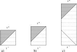
Figure 1: Conformal diagrams of a) de Sitter space, b) perturbed de Sitter space, and c) a very tall asymptotically de Sitter spacetime. The worldline of the ‘central observer’ is the right boundary of each diagram and various horizons related to her worldline are shown. Shaded regions cannot send signals to this observer.

An interesting property of de Sitter space is that it has compact Cauchy surfaces. However, as illustrated in figure 1(a), the causal structure of pure de Sitter space is such that an observer can never see an entire compact Cauchy surface. Instead, the observer’s light cone only expands to include the full Cauchy surface at $I^{-}$, asymptotically as the observer approaches $I^{+}$ . This causal connection between $I^{+}$ and $I^{-}$ plays an important role in understanding the role of both of these surfaces in the dS/CFT correspondence [2, 5, 6, 7]. However, a theorem (Corollary 1) of Gao and Wald [14] tells us that under a generic perturbation of de Sitter space, the conformal diagram becomes taller so that an entire compact Cauchy surface now becomes visible at some finite time. This is shown in figure 1(b). Pushing this somewhat further, one can imagine that in certain circumstances asymptotically de Sitter spacetimes of the sort shown in figure 1(c) may arise. That is, in these spacetimes, a compact Cauchy surface lies in the intersection of the past and future of a generic worldline. In fact, we construct explicit examples of such spacetimes in section 6. These particular examples are of some interest with regard to general discussions of ‘the number of degrees of freedom’ in asymptotically de Sitter spaces [8, 16, 17], as the region open to experimental probing by an observer contains arbitrarily large spatial volumes.

The primary focus of the present paper is investigating renormalization group flows in the context of the dS/CFT duality. The paper is organized as follows: In section 2, we review the basics of de Sitter space, establish our conventions, and introduce the three types of foliations (spherical, flat, and hyperbolic) that will be most relevant in the following sections. Section 3 then generalizes to include a rolling scalar field, which may yield ‘flows’ which are asymptotically dS. In particular, we describe two solution generating techniques which may be used to construct explicit solutions. Section 4 is devoted to extending the ‘c-theorem’ for asymptotically de Sitter evolutions [3, 4]. We generalize the ‘c-theorem’ to include flows with spherical or hyperbolic spatial sections and also certain situations where the spatial geometries are anisotropic. We find that under these general circumstances, an ‘effective’ cosmological constant always decreases (increases) during an expanding (contracting) phase. Finally we consider the possibilities for transitions between phases of expansion and contraction. Because of our interest in global structures, we discuss the Penrose diagrams relevant to these flows in section 5. Section 6 describes the construction of a ‘very tall’ universe. Within the context of one model, we illustrate solutions with asymptotically de Sitter regions both to the future and past and that contain an arbitrarily long lived intermediate matter dominated phase in which the spatial volume is arbitrarily large. We conclude with a discussion of our results in section 7. Finally, with three appendices, we provide additional examples of asymptotically de Sitter renormalization group flows, and flesh out the construction of the conformal diagrams discussed in section 5.

2 De Sitter space basics

The simplest construction of the ($n$+1)-dimensional de Sitter (dS) spacetime is through an embedding in Minkowski space in $n+2$ dimensions, where it may be defined as the hyperboloid

$$\eta_{AB}X^{A}X^{B}=\ell^{2}.$$ (1)

The resulting surface is maximally symmetric, i.e.,

$$R_{ijkl}={1\over\ell^{2}}(g_{ik}\,g_{jl}-g_{il}\,g_{jk})\ ,$$ (2)

which also ensures that the geometry is locally conformally flat. Hence dS space solves Einstein’s equations with a positive cosmological constant,

$$R_{ij}={2\Lambda\over n-1}g_{ij}\qquad{\rm with}\quad\Lambda={n(n-1)\over 2\ell^{2}}\ .$$ (3)

The topology of the space is $R\times S^{n}$. The Penrose diagram is represented by a square [18], as illustrated in Figure 1 (a). Any horizontal cross section of the figure is an $n$-sphere, so that any point in the interior of the diagram represents an $(n-1)$-sphere. At the right and left edges, the points correspond to the north and south poles of the $n$-sphere. Note that diagram is just tall enough that a null cone emerging from, say, the south pole at $I^{-}$ reconverges on the north pole at $I^{+}$.

One may present the metric on dS space in many different coordinate systems, which may be particularly useful in different situations. Three simple choices for ($n$+1)-dimensional dS space come from foliating the embedding space above with flat hypersurfaces, $n_{A}X^{A}=constant$. The three distinct choices correspond to the cases where the normal vector $n_{A}$ is time-like, null or space-like. With these distinct choices, a given hypersurface intersects the hyperboloid on a spatial section which has a spherical, flat or hyperbolic geometry, respectively. Following the standard notation for Friedmann-Robertson-Walker cosmologies, we denote these three cases as $k=+1,0$ and $-1$, respectively. Then the three corresponding metrics on dS space can be written in a unified way as follows:

$$ds^{2}=-dt^{2}+a_{k}^{2}(t)d\Sigma^{2}_{k,n}\ ,$$ (4)

where the $n$-dimensional Euclidean metric $d\Sigma^{2}_{k,n}$ is

$$d\Sigma^{2}_{k,n}=\left\{\begin{array}[]{ll}\vphantom{\sum_{i=1}^{n}}\ell^{2}d\Omega^{2}_{n}&{\rm for}\;k=+1\\ \sum_{i=1}^{n}dx_{i}^{2}&{\rm for}\;k=0\\ \vphantom{\sum_{i=1}^{n}}\ell^{2}d\Xi^{2}_{n}&{\rm for}\;k=-1\ ,\end{array}\right.$$ (5)

where $d\Omega^{2}_{n}$ is the unit metric on $S^{n}$. The ‘unit metric’ $d\Xi^{2}_{n}$ is the $n$–dimensional hyperbolic space ($H^{n}$) which can be obtained by analytic continuation of that on $S^{n}$. For $k{=}\pm 1$ we assume that $n\geq 2$.

The scale factor in each of these cases would be given by

$$a_{k}(t)=\left\{\begin{array}[]{lll}\cosh(t/\ell)&{\rm for}\;k=+1\\ \exp({t/\ell})&{\rm for}\;k=0\\ \sinh(t/\ell)&{\rm for}\;k=-1\ .\end{array}\right.$$ (6)

Hence we see that $k=+1$ corresponds to the standard global coordinates, in which the spatial $n$-sphere begins by shrinking from infinity to a minimum size (with radius $\ell$) and then it re-expands. The choice $k=0$ corresponds to the standard inflationary coordinates, where the flat spatial slices experience an exponential expansion (assuming a positive sign in the exponential). In this case, $t=-\infty$ corresponds to a horizon (i.e., the boundary of the causal future) for a co-moving observer emerging from $I^{-}$. Hence these coordinates only cover half of the full dS space but, of course, substituting a minus sign in the exponential of eq. (6) yields a metric which naturally covers the lower half. The choice $k=-1$ yields a perhaps less familiar coordinate choice where the spatial sections have constant negative curvature. In this case, $t=0$ again represents a horizon. However, this horizon is the future null cone of an actual point inside dS space. Figure 2 illustrates slices of constant $t$ on a conformal diagram of dS space. It is straightforward to see that all of the above coordinate systems in fact are related by a local diffeomorphism. One might also note the exponential expansion that dominates the late time evolution of all three slicings independent of the spatial curvature, i.e., $a_{k}(t)\sim exp(t/\ell)$ as $t\rightarrow\infty$ for all $k$.

These three different coordinate patches are displayed on the full Penrose diagram in figure 2. One comment on the $k=-1$ case is that the central diamond cannot be foliated by homogeneous spacelike hyperboloids. However, it is naturally foliated by timelike hyperboloids, i.e., by copies of dS space. The metric in the central diamond region may be obtained by double analytic continuation of (4) and the result is

$$ds^{2}=dt^{2}+\ell^{2}\sin^{2}(t/\ell)ds^{2}_{dS},$$ (7)

where $ds^{2}_{dS}$ is the metric for $n$-dimensional de Sitter space with unit radius of curvature. Here $t$ is a spacelike coordinate that is naturally thought of as the analytic continuation of the $t$ in (6) behind the horizon.

Figure 2: Constant $t$ slices in a) the spherical slicing, b) the flat slicing, and c) the hyperbolic slicing of de Sitter space.

With the metric (4), we have apparently displayed dS_n+1 with three different boundary geometries:

$$S^{n},\quad{\hbox{{\rm I}\kern-1.99997pt\hbox{\rm R}}}^{n}\quad{\rm and}\quad H^{n}\ .$$ (8)

The dS/CFT correspondence would imply then an equivalence between, on the one hand, quantum gravity in dS space and a CFT on any of the above backgrounds (8). On the other hand, we know that the (past and future) timelike infinities of dS_n+1 space have the topology $S^{n}$. Hence the correct observation is that the latter two boundary geometries are equivalent to (a portion of) $S^{n}$ up to a conformal transformation. However, a singularity in the latter transformation effectively removes (i.e., pushes off to infinity) certain points on the sphere to produce the resulting geometry. In the case where the boundary appears to be $H^{n}$, it is obvious from the Penrose diagram (see figure 2) that these coordinates cover only half of the boundary of dS space. Hence the conformal transformation has pushed out the equator of the boundary sphere to produce two copies of the hyperbolic plane.

A common feature of the three coordinate systems (4) above is that the spatial geometry is uniformly scaled in the time evolution. In appendix A, we present some other metrics on dS space which have non-uniform scalings. In particular, the boundary metric takes the form of a direct product of two submanifolds and each of the latter submanifolds evolves with a different scale factor.

3 Generating asymptotically de Sitter solutions

In this section, we set forth a framework in which to consider generalized dS flows or asymptotically dS solutions. In investigating new phenomena, it is useful to have a set of explicit solutions at one’s disposal. Hence, we introduce two solution generating techniques below. Section 3.1 describes a method that allows for a variety of potentials but is useful mainly for the case of spatially flat sections ($k=0$). This approach is a simple adaptation of the techniques developed in [19] for the case of spatially varying solutions with a negative cosmological constant. This approach allows the equations of motion to be reduced to two first order ODE’s. Section 3.2 treats the special case of piece-wise constant potentials in a way that remains useful for any value of $k$. Throughout this section, our attention is restricted to spacetimes with homogeneous spatial sections.

In general we consider $(n+1)$-dimensional models of Einstein gravity coupled to a scalar field $\phi$. We write the action as

$$S=\frac{1}{16\pi G_{\scriptscriptstyle N}}\int d^{n+1}x\sqrt{-g}\,\left[R-n(n-1)g^{ij}\partial_{i}\phi\partial_{j}\phi-n(n-1)V(\phi)\,\right]\ .$$ (9)

Note that the scalar field terms have been normalized in an unconventional manner (including the fact that Newton’s constant $G_{\scriptscriptstyle N}$ appears in an overall factor in front of the total action) to simplify Einstein’s equations in the following analysis. Einstein’s equations may be written as

$$R_{ij}-\frac{1}{2}g_{ij}R=T_{ij},$$ (10)

where the stress-energy tensor is given (with a slightly unconventional normalization) as

$$T_{ij}=n(n-1)\left[\partial_{i}\phi\partial_{j}\phi-\frac{1}{2}g_{ij}\left(\,(\partial\phi)^{2}+V(\phi)\,\right)\,\right]\ .$$ (11)

Note that if the scalar field sits at a critical point $\phi=\phi_{0}$ of the potential $V(\phi)$, the effective cosmological constant is given by $\Lambda=\frac{n(n-1)}{2}V(\phi_{0})$.

Now we will consider the spatially homogeneous solutions of the form

$$\phi=\phi(t)\quad{\rm and}\quad ds^{2}=-dt^{2}+a^{2}(t)d\Sigma^{2}_{k,n}$$ (12)

with $d\Sigma^{2}_{k,n}$ defined in eq. (5). Given this ansatz, the scalar field equation reduces to

$$\ddot{\phi}+n\frac{\dot{a}}{a}\dot{\phi}=-\frac{1}{2}\frac{\partial V}{\partial\phi}\ ,$$ (13)

where a ‘dot’ denotes a derivative with respect to $t$. The dynamics of the scale factor $a(t)$ is governed by the Friedmann equations

$$\left(\frac{\dot{a}}{a}\right)^{2}+\frac{k}{a^{2}}=\dot{\phi}^{2}+V(\phi)\ ,$$ (14)

$$\frac{\ddot{a}}{a}=-(n-1)\dot{\phi}^{2}+V(\phi)\ .$$ (15)

The second of these is redundant, and a complete solution may be determined from eqs. (13) and (14) alone.

3.1 Pre-potentials

One approach to producing explicit solutions is to adapt the technique of [19] to the present case. This method considers potentials of a special form which allow us to simplify the equations of motion, (13) and (14), for both $a(t)$ and $\phi(t)$ to a system of two first order ODE’s. It is easily verified that eqs. (13), (14) and (15) are satisfied when $\phi$, $\dot{a}/a$, and $V(\phi)$ are related to a pre-potential $W(\phi)$ through

$$\dot{\phi}=\frac{1}{\gamma}\frac{\partial W(\phi)}{\partial\phi}\;\;\;\;\;\;\frac{\dot{a}}{a}=-\gamma nW(\phi),$$ (16)

$$V(\phi)=-\frac{1}{\gamma^{2}}\left(\frac{\partial W(\phi)}{\partial\phi}\right)^{2}+n^{2}W^{2}(\phi),$$ (17)

where

$$\gamma=\left(1-\frac{k}{n^{2}W(\phi)^{2}a^{2}}\right)^{1/2}.$$ (18)

For $k=\pm 1$, these expressions are of limited use as they are highly nonlinear and further the scale factor $a(t)$ appears in eq. (17) through the factor of $\gamma^{2}$. However, for $k=0$, $\gamma=1$ and the scalar potential is completely determined by the pre-potential $W(\phi)$. In this case, the equations (16) reduce to

$$\dot{\phi}=\frac{\partial W(\phi)}{\partial\phi}\;\;\;\;\;\;\frac{\dot{a}}{a}=-nW(\phi)\ ,$$ (19)

which can readily be solved analytically given a sufficiently simple $W(\phi)$. While this technique allows us to construct many interesting analytic flows, we will not consider any explicit examples here.

3.2 Step potentials

Another class of tractable models arises when $V(\phi)$ is piece-wise constant. On each constant piece, the system can be mapped to a particle in a one-dimensional potential so that the dynamics is conveniently summarized by the effective potential. One may then patch together the solutions at the boundaries of the steps. With some number of small steps, this approach may be useful to approximate a slowly varying potential. Alternatively, this technique may be used to simulate the effect of phase transitions in the matter sector. We will consider an interesting example based on these models in section 6.

Let us first consider the dynamics within one step with constant $V(\phi)=V_{0}$, which is assumed to be positive. Recall that in this phase of the evolution, the cosmological constant is given by $\Lambda=n(n-1)V_{0}/2$. From (13), the scalar field equation reduces to

$$0=\ddot{\phi}+n\frac{\dot{a}}{a}\dot{\phi}=a^{-n}\frac{\partial}{\partial t}(a^{n}\dot{\phi}).$$ (20)

Thus, we introduce an integration constant $C_{0}=a^{n}\dot{\phi}$. The familiar Friedmann constraint (14) may then be rewritten as

$$-k=\dot{a}^{2}+w_{eff}(a)\qquad{\rm where}\quad w_{eff}(a)=-\frac{C_{0}^{2}}{a^{2(n-1)}}-V_{0}a^{2}\ .$$ (21)

Hence we may view the dynamics of the scale factor $a$ as that of a classical particle moving in a potential $w_{eff}$ with energy $-k$.

Note that if $C_{0}\not=0$, the effective potential is manifestly negative. However, for the flat and hyperbolic cases ($k=0,-1$), the effective energy is non-negative. Hence for all such solutions, the scale factor reaches zero in either the past or future. Further with $C_{0}\not=0$, one finds a curvature singularity at this point: $a\sim t^{1/n}$ and $R\simeq-{n\over n+1}t^{-2}$. Hence these solutions correspond either to a universe which begins in a contracting dS phase and for which there is enough energy density in the evolving scalar field to produce a big crunch singularity, or similarly to a universe which emerges from a big bang to evolve into an expanding dS phase. Of course, with $C_{0}=0$, the scale factor $a$ reaches zero in a non-singular way which simply corresponds to a horizon in dS space, as discussed above.

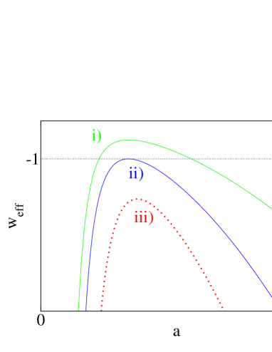
Figure 3: The effective potential $w_{eff}$ with $n=3,k=+1$ for three different cases: i) small $C_{0}^{2}V_{0}^{2}$, ii) $C_{0}^{2}V_{0}^{2}=\frac{4}{27}$, and iii) large $C_{0}^{2}V_{0}^{2}.$

However, the spherical case ($k{=}+1$) is more interesting since the effective energy is negative. For $C_{0}^{2}>V_{0}^{-(n-1)}\frac{1}{n-1}\left(\frac{n-1}{n}\right)^{n}$, one has $w_{eff}<-1$ for all values of $a$. Hence the solutions in this range have a similar interpretation as above with a big crunch or big bang singularity. With $C_{0}^{2}=V_{0}^{-(n-1)}\frac{1}{n-1}\left(\frac{n-1}{n}\right)^{n}$, the peak of the effective potential is precisely $-1$, and so there are various classes of solutions: i) the scale factor is constant with $a^{2n}=V_{0}^{-n}\left(\frac{n-1}{n}\right)^{n}$ and the geometry corresponds to an Einstein static universe, ii) the universe emerges from a big bang and asymptotically evolves toward the previous static geometry, iii) the universe begins with a contracting dS phase and asymptotically approaches the static phase above, and iv) the time reversal of the solutions in either (ii) or (iii). For smaller values of $C_{0}$, the universe is confined either to small $a$ (leading to solutions having both a big bang and a big crunch) or to large $a$ (with dS phases both to the past and future). In all cases, $\phi$ rolls monotonically in one direction.

A piece-wise constant potential can now be dealt with by patching together solutions described by the above effective potentials. When $\phi$ crosses a jump in the potential $V$, the equations of motion show that $a$, $\dot{a}$, and $\phi$ are continuous but that $\dot{\phi}$ and $\ddot{a}$ suffer a discontinuity. The Friedmann constraint (14) then shows that this discontinuity is determined by the requirement that the scalar field energy density $\dot{\phi}^{2}+V$ is conserved through the transition. That is, the two solutions are pasted together such that the effective potential is continuous across the join. As a result, the integration constants $C_{1},C_{2}$ associated with potentials $V_{1},V_{2}$, respectively satisfy the constraint:

$$C_{2}^{2}+V_{2}a^{2n}=C_{1}^{2}+V_{1}a^{2n}\ .$$ (22)

This analysis will be used in the construction of a ‘very tall’ universe in section 6.

4 A generalized de Sitter c-theorem

Having illustrated a framework in which we may study asymptotically dS spaces which are more general than the original dS spacetime, we would like to consider the role of such solutions in the context of the dS/CFT correspondence [2]. Much of the development of this duality relies on intuition developed in studying the AdS/CFT correspondence [20]. One of the interesting features of the latter is the UV/IR correspondence [21, 22]. That is, physics at large (small) radii in the AdS space is dual to local, ultraviolet (nonlocal, infrared) physics in the dual CFT. As was extensively studied in gauged supergravity — see, e.g., [23] — ‘domain wall’ solutions which evolve from one phase near the AdS boundary to another in the interior can be interpreted as renormalization group flows of the CFT when perturbed by certain operators. In analogy to Zamolodchikov’s results for two-dimensional CFT’s [24], it was found that a c-theorem could be established for such flows [25] — see also [26] — using Einstein’s equations. The c-function defined in terms of the gravity theory then seems to give a local geometric measure of the number of degrees of freedom relevant for physics at different energy scales in the dual field theory.

In the dS/CFT duality, there is again a natural correspondence between UV (IR) physics in the CFT and phenomena occurring near the boundary (deep in the interior) of dS space. In the context then of more general solutions which are asymptotically dS, one has an interpretation in terms of renormalization group flows, which should naturally be subject to a c-theorem [3, 4]. The original investigations [3, 4] considered only solutions with flat spatial sections ($k=0$), and we generalize these results in the following to include spherical and hyperbolic sections ($k=\pm 1$). We also consider the flows involving anisotropic scalings of the boundary geometry, but our results are less conclusive in this case.

4.1 The c-function

The foliations of spacetimes of the form given in eq. (12) are privileged in that time translations a) act as a scaling on the spatial metric, and thus in the field theory dual and b) preserve the foliation and merely move one slice to another. In the context of the dS/CFT correspondence, these properties naturally lead to the idea that time evolution in these spaces should be interpreted as a renormalization group flow [3, 4]. Certainly, the same properties apply for time evolution independent of the curvature of the spatial sections, and in fact also apply (in the asymptotically dS regions) for any of the metrics presented in Appendix A. Hence if a c-theorem applies for the $k=0$ solutions [3, 4], one might expect that it should extend to these other cases if properly generalized.

For $k=0$, the proposed c-function [3, 4], when generalized to $n{+}1$ dimensions, is

$$c\simeq{1\over G_{\scriptscriptstyle N}\left|{\dot{a}\over a}\right|^{n-1}}\ .$$ (23)

The Einstein equations ensure that $\partial_{t}\left(\dot{a}/a\right)<0$, provided that any matter in the spacetime satisfies the null energy condition [18]. This result then guarantees that $c$ will always decrease in a contracting phase of the evolution or increase in an expanding phase.

For our general study, we wish to define a c-function which can be evaluated on each slice of some foliation of the spacetime. Of course, our function should satisfy a ‘c-theorem’, e.g., our function should monotonically decrease as the surfaces contract in the spacetime evolution. Further, it should be a geometric function built from the intrinsic and extrinsic curvatures of a slice. Toward this end, we begin with the idea that the c-function is known for any slice of de Sitter space, and note that in this case, eq. (23) takes the form

$$c\sim{1\over G_{\scriptscriptstyle N}\Lambda^{(n-1)/2}}\ .$$ (24)

Thus, if our slice can be embedded in some de Sitter space (as was shown to be the case for any isotropic homogeneous slice in section 2), the value of the c-function should be given by eq. (24). In other words, we can associate an effective cosmological constant $\Lambda_{eff}$ to any slice that can be embedded in de Sitter space and we can then use this $\Lambda_{eff}$ to define our c-function.

It is useful to think a bit about this embedding in order to express $\Lambda_{eff}$ directly in terms of the intrinsic and extrinsic curvatures of our slice. The answer is readily apparent from the general form of the ‘vacuum’ Einstein equations with a positive cosmological constant: $G_{ij}=-\Lambda g_{ij}$. Contracting these equations twice along the unit normal $n^{i}$ to the hypersurface gives the Hamiltonian constraint, which is indeed a function only of the intrinsic and extrinsic curvature of the slice. The effective cosmological constant defined by such a local matching to de Sitter space is therefore given by

$$\Lambda_{eff}=G_{ij}n^{i}n^{j}.$$ (25)

For metrics of the general form (4), this becomes

$$\Lambda_{eff}=\frac{n(n-1)}{2}\left[\left(\frac{\dot{a}}{a}\right)^{2}+{k\over a^{2}}\right].$$ (26)

Taking the c-function to be a function of this effective cosmological constant, dimensional analysis then fixes it to be

$$c\sim\frac{1}{G_{\scriptscriptstyle N}\Lambda_{eff}^{(n-1)/2}}=\frac{1}{G_{\scriptscriptstyle N}}\left({G_{ij}n^{i}n^{j}}\right)^{-(n-1)/2}\ .$$ (27)

For the $k=0$ isotropic case, it is clear that this reduces to the c-function (23) given previously in [3, 4]. For other isotropic cases, it is uniquely determined by the answer for the corresponding slices of de Sitter space. The same holds for an anisotropic slice that can be embedded in de Sitter (see e.g. Appendix A for examples). While the choice (27) is not uniquely determined by the constraints imposed thus far for any slice which cannot be so embedded, it does represent a natural generalization and, as we will see below, this definition allows a reasonable ‘c-theorem’ to be proven.

4.2 The c-theorem

For any of the homogeneous flows as considered in the previous section, it is straightforward to show that our c-function (27) always decreases (increases) in a contracting (expanding) phase of the evolution. However, we would like to give a more general discussion which in particular allows us to consider anisotropic geometries, as well as these isotropic cases.

To prove our theorem, we note that the Einstein equations relate our effective cosmological constant to the energy density $\rho$ on the hypersurface,

$$\Lambda_{eff}=G_{ij}\,n^{i}n^{j}=T_{ij}\,n^{i}n^{j}=\rho.$$ (28)

Consider now the ‘matter energy’ $E=\rho V$ contained in the volume $V$ of a small co-moving rectangular region on the homogeneous slice. That is, we take

$$V=\int_{R}\sqrt{g}\,d^{n}x$$ (29)

for some small co-moving region $R$ of the form $R=\{x|x^{i}_{a}<x^{i}<x^{i}_{b}\}$ where $x^{i}$ denote co-moving spatial coordinates. We also introduce $\delta x^{i}=x^{i}_{b}-x^{i}_{a},$ the co-moving size of $R$ in the $i$th direction. Since $R$ is small, each coordinate $x^{i}$ can be associated with a scale factor $a^{i}(t)$ such that the corresponding physical linear size of $R$ is $a^{i}(t)\delta x^{i}.$

Without loss of generality, let us assume that the coordinates $x^{i}$ are aligned with the principle pressures $P_{i}$, which are the eigenvalues of the stress tensor on the hypersurface. Let us also introduce the corresponding area $A_{i}$ of each face. Note that a net flow of energy into $R$ from the neighboring region is forbidden by homogeneity. As a result, energy conservation implies that $dE=-P_{i}A_{i}d(a\delta x^{i})$ as the slice evolves. However, clearly $dE=\rho dV+Vd\rho$, so that we have

$$d\Lambda_{eff}=d\rho=-\sum_{i}\left(\rho+P_{i}\right)d\ln a_{i}.$$ (30)

Now we will assume that any matter fields satisfy the weak energy condition so that $\rho~{}+~{}P_{i}~{}\geq~{}0$. Thus, if all of the scale factors are increasing, we find that the effective cosmological constant can only decrease in time.

This result provides a direct generalization of the results of [3, 4] to slicings that are not spatially flat. In particular, in the isotropic case (where all scale factors are equal, $a\equiv a_{i}=a_{j}$), it follows that $c(a)$ as given in eq. (26) is, as desired, a monotonically increasing function in any expanding phase of the universe.

Note, however, that the anisotropic case is not so simple to interpret. For example, it maybe that the scale factors are expanding in some directions and contracting in others. In this case our effective cosmological constant may either increase or decrease, depending on the details of the solution.

4.3 Complete Flows versus Bouncing Universes

The general flows are further complicated by the fact that they may ‘bounce’, i.e., the evolution of the scale factor(s) may reverse itself. The simplest example of this would be the $k{=}+1$ foliation of dS space in section 2. In this global coordinate system, the scale factor (6) begins contracting from $a(t=-\infty)=\infty$ to $a(t=0)=1$, but then expands again toward the asymptotic region at $t=+\infty$. In contrast, we refer to the $k{=}0$ and –1 foliations as ‘complete’. By this we mean that within a given coordinate patch, the flow proceeds monotonically from $a=\infty$ in the asymptotic region to $a=0$ at the boundary of the patch — the latter may be either simply a horizon (as in the case of pure dS space) or a true curvature singularity.

For any homogeneous flows, such as those considered in section 3, it is not hard to show that the $k{=}0$ and –1 flows are always complete and that only the $k{=}+1$ flows can bounce. The essential observation is that for $a(t)$ to bounce the Hubble parameter $\dot{a}/a$ must pass through zero. Now the ($tt$)-component of the Einstein equations (10) yields

$$\left({\dot{a}\over a}\right)^{2}=T_{tt}-{k\over a^{2}}\ .$$ (31)

Now as long as the weak energy condition applies, it is clear that the right-hand-side is always positive for $k=0$ and –1 and so $\dot{a}/a$ will never reach zero. On the other hand, no such statement can be made for $k{=}+1$ and so it is only in this case that bounces are possible. Further one might observe that this analysis does not limit the number of bounces which such a solution might undergo. In certain cases with a simple matter content, e.g., dust or radiation, one may show that only a single bounce is possible. However in (slightly) more complex models, multiple bounces are possible. We will illustrate this behavior in section 6, where a solution with a rolling scalar is constructed with multiple bounces — see also appendix B. Finally in the case of anisotropic solutions — see, e.g., Appendix A — the characterization of the flows as complete or otherwise is more complicated.

The renormalization group interpretation of bouncing universes is certainly less straightforward. Perhaps greater insight into this question can come from further study of renormalization group flows and the UV/IR correspondence in the AdS/CFT context for foliations of AdS space where the sections have negative curvature. Such AdS solutions show a similar bounce behavior — see, e.g., [27].

5 The global perspective

Recall from the introduction the observation that asymptotically de Sitter conformal diagrams are ‘tall’, i.e., an entire compact Cauchy surface will be visible to observers at some finite time, and hence that perturbations of dS space may bring features that originally lay behind a horizon into an experimentally accessible region. Specifically, these results rely on Corollary 1 of [14], which we paraphrase as follows:

Let the spacetime $(M,g_{ij})$ be null geodesically complete and satisfy the weak null energy condition and the null generic condition. Suppose in addition that $(M,g_{ij})$ is globally hyperbolic with a compact Cauchy surface $\Sigma$. Then there exist Cauchy surfaces $\Sigma_{1}$ and $\Sigma_{2}$ (of the same compact topology, and with $\Sigma_{2}$ in the future of $\Sigma_{1}$) such that if a point $q$ lies in the future of $\Sigma_{2}$, then the entire Cauchy surface $\Sigma_{1}$ lies in the causal past of $q$.

This is sufficient to guarantee that the conformal diagram is ‘tall’ in the sense of figure 1 (b). While it need not necessarily be ‘very tall’ in the sense of figure 1 (c), the possibility is open that this may hold in certain cases so that a compact Cauchy surface may actually be found to lie within the intersection of the past and future of a generic worldline. An example of such a spacetime will be constructed in section 6 below.

The diagrams in figure 1 were not intended to represent generic asymptotically de Sitter spacetimes. Instead, these diagrams only illustrate what is meant by ‘tall’ and ‘very tall’ spacetimes. The purpose of the current section is to construct the general such conformal diagrams corresponding to our homogeneous flows. This may be of particular interest if in the end there is a meaningful dS/CFT correspondence in which (either distinct or isomorphic) field theories are associated with both $I^{+}$ and $I^{-}$. We note that two field theories are indeed of relevance to certain applications [28, 29] of the more developed AdS/CFT correspondence.

Although we have shown that the evolution of $c(a)$ is monotonic, certain unusual features of our flow become apparent when we study the global structure of the spacetimes dual to our field theory. Let us assume that the slices are isotropic and take each of the three possible cases (spheres, flat slices, and hyperbolic slices) in turn.

5.1 Flat slices ($k=0$)

We now wish to construct the conformal diagram for flows with flat spatial sections. In order to draw useful two-dimensional diagrams, we shall use the common trick of studying rotationally symmetric spacetimes and drawing conformal diagrams associated with the ‘$r$-$t$ plane,’ i.e., associated with a hypersurface orthogonal to the spheres of symmetry.

Figure 4: In the distant past $\tau$ is a) finite b) infinite.

For later use, we begin with an arbitrary $n+1$ dimensional spatially homogeneous and spherically symmetric metric in proper time gauge:

$$ds^{2}=-dt^{2}+a^{2}(t)\left(dr^{2}+\hat{R}^{2}(r)d\Omega^{2}_{n-1}\right),$$ (32)

where $d\Omega^{2}_{n-1}$ is the metric on the unit $n-1$ sphere and the form of $\hat{R}(r)$ depends on the spatial geometry: $\hat{R}(r)=\sin(r),r,\sinh(r)$ for spherical, flat, and hyperbolic geometries respectively. In fact, the function $\hat{R}(r)$ will not play a role below as our diagrams will depict the conformal structure only of the ($1+1$)-dimensional metric $ds^{2}_{1+1}=-dt^{2}+a^{2}(t)dr^{2}.$ However, it will be important to note that $r$ takes values only in $[0,\pi]$ for the spherical geometry but takes values in $[0,\infty]$ for the flat and hyperbolic cases. The usual change of coordinates to conformal time $\tau(t)$ defined by $d\tau=\frac{dt}{a}$ leads to the conformally Minkowski metric

$$ds^{2}_{1+1}=a^{2}(t)(-d\tau^{2}+dr^{2}).$$ (33)

Let us assume that our foliation represents an expanding phase that is asymptotically de Sitter in the far future. That is, for $t\rightarrow+\infty$ the scale factor $a$ diverges exponentially. There are now two possibilities. Suppose first that $a=0$ at some finite $t$. If $a^{-1}$ diverges as a small enough power of $t$ then $\tau$ will only reach a finite value in the past and the spacetime is conformal to a half-strip in Minkowski space.

In contrast, if $a$ vanishes more quickly or if it vanishes only asymptotically then $\tau$ can be chosen to take values in $[-\infty,0]$. From (33) we see that the region covered by our foliation is then conformal to a quadrant of Minkowski space. We take this quadrant to be the lower left one so that we may draw the conformal diagram as in figure 4 (b).

We now wish to ask whether the region shown in figure 4 (b) is ‘complete’ in some physical sense. In particular, we may wish to know whether light rays can reach the null ‘boundary’ in finite affine parameter. A short calculation shows that the affine parameter $\lambda$ of a radial null ray is related to the original time coordinate $t$ by $d\lambda=adt.$ The affine parameter is clearly finite if $a$ vanishes at finite $t$. In the remaining case, we have seen that $\rho$ is bounded below. As a result, $a$ must vanish at least exponentially and the affine parameter is again finite.

Figure 5: a) In a square diagram, a light ray reaches the antipodal point only at $I^{+}$. b) The generic conformal diagram for an asymptotically de Sitter space with flat surfaces of homogeneity. A light ray starting in the lower left corner reaches the antipodal point at a finite time.

Thus, this null surface represents either a singularity or a Cauchy horizon across which our spacetime should be continued. This statement is essentially a restricted version of the results of [30, 31, 32, 33] (see also [34] for other interesting constraints on the ‘beginning’ of inflation). Note that there is no tension between our possible Cauchy horizon and the claim of a “singularity” in these references, as their use of the term singularity refers only to the geodesic incompleteness of the expanding phase.

From (30) we see that unless $\rho+P_{i}$ vanishes as $a\rightarrow 0$, the energy density must diverge and a curvature singularity will indeed result. However, a proper tuning of the matter fields can achieve a finite $\rho$ at $a=0$. It is therefore interesting to consider solutions which are asymptotically de Sitter near $t=0$ so that $a$ vanishes exponentially. In this case, the $a=0$ surface represents a Cauchy horizon across which we should continue our spacetime. We will focus exclusively on such cases below.

Since the boundary is a Cauchy horizon, there is clearly some arbitrariness in the choice of extension. We make the natural assumption here that the spacetime beyond the horizon is again foliated by flat hypersurfaces. Although at least one null hypersurface ($t=-\infty$) will be required, it can be shown that the surfaces of homogeneity must again become spacelike across the horizon if the spacetime is smooth. The key point here is that the signature can be deduced from the behavior of $a^{2}(t)$, which gives the norm $|\xi|^{2}$ of any Killing vector field $\xi$ associated with the homogeneity. We impose a “past asymptotic de Sitter boundary condition” so that the behavior of this quantity near the Cauchy horizon must match that of some de Sitter spacetime. Consider in particular the behavior along some null geodesic crossing the Cauchy horizon and having affine parameter $\lambda$. It is straightforward to verify that $\lambda\sim a$, so that matching derivatives of $|\xi|^{2}$ across the horizon requires $\xi$ to again become spacelike beyond the horizon.

It follows that the region beyond the Cauchy surface is just another region of flat spatial slices, but this time in the contracting phase. It is therefore conformal to the upper right quadrant of Minkowski space. However, having drawn the above diagram for our first region we have already used a certain amount of the available conformal freedom. Thus, it may not be the case that the region beyond the Cauchy surface can be drawn as an isosceles right triangle. The special case where this is possible is shown in figure 5 (a). The exceptional nature of this case can be seen from the fact that it allows a spherical congruence of null geodesics to proceed from the upper right corner of $I^{+}$ (where it would have zero expansion) to the lower right corner of $I^{-}$ (where it would also have zero expansion). Assuming as usual the weak energy condition, it follows that this congruence encountered no focusing anywhere along its path; i.e., $\rho+P=0$. Given the high degree of symmetry that we have already assumed, this can happen only in pure de Sitter space. The correct diagram for the general case is shown in figure 5 (b) (see appendix C for a complete derivation).

Figure 6: Conformal diagrams for spherical surfaces of homogeneity a) for the case where $\tau$ diverges in the past and b) for the case where $\tau$ converges in the past.

5.2 Spherical slices ($k=+1$)

The conformal diagrams in this case are relatively simple. Since the radial coordinate now takes values only in an interval, we see from (33) that the conformal diagram is either a rectangle or a half-vertical strip, depending on whether or not $\tau$ is finite at the past boundary.

All such rectangles with the same ratio h/w (see figure 6 (b)) can be mapped into each other via conformal transformations. For the case of pure de Sitter space we have h=w. On the other hand, for any spacetime satisfying the generic condition (so that null geodesics suffer some convergence along their trajectory), we know from [14] that the region to the past of any point $p$ sufficiently close to $I^{+}$ must contain an entire Cauchy surface. Thus, for such cases we have h $>$ w. Similar ‘tall’ spacetimes were recently considered in the context of cosmologies violating the dominant energy condition [35].

5.3 Hyperbolic slices ($k=-1$)

Figure 7: The general conformal diagram for an appropriately complete asymptotically de Sitter spacetime with hyperbolic surfaces of homogeneity. A conformal frame has been chosen such that the diagram has a $Z_{2}$ reflection symmetry through the center.

Recall that the hyperbolic flows are complete, i.e., $a$ reaches 0 at finite $t$ (say, $t=0$), and vanish at least as fast as $t$. The asymptotically de Sitter boundary conditions also require that $a$ diverge exponentially as $t\rightarrow+\infty$. Note that since $a$ vanishes quickly, $\tau$ will diverge at $t=0$ and the region is again conformal to a quadrant of Minkowski space. As usual, this may or may not be singular depending on the matter present.

Consider in particular the asymptotically de Sitter case where $a$ vanishes linearly. One then finds that the affine parameter $\lambda$ along a null ray near the horizon is asymptotically $\lambda\sim a^{2}$. The Killing vector field that implements spatial translations in the direction along this null ray has a norm given by $a^{2}\sim\lambda$ along this null ray and so, if the spacetime is smooth, must become timelike beyond the horizon. Thus, the homogeneous surfaces must become timelike on the other side. As can be seen from (7), an asymptotically de Sitter region foliated by timelike hyperbolic slices (i.e., copies of de Sitter space) has an ‘r-t plane’ that is conformal to a diamond in Minkowski space.

Assuming that no singularities are encountered within this diamond or on its boundaries, this provides three further Cauchy horizons across which we would like to extend our spacetime. A study of the norm of the Killing fields tells us that the foliation must again become spacelike beyond these horizons. Just as we saw for the flat foliations, we are therefore left with the task of attaching pieces conformal to various quadrants of Minkowski space. By the same reasoning as in appendix C, the complete conformal diagram can be drawn as shown in figure 7.

6 ‘Very tall’ universes

This section is devoted to constructing an asymptotically de Sitter spacetime whose conformal diagram is ‘tall’ enough that a compact Cauchy surface can be experimentally probed by a co-moving observer. In particular, such a Cauchy surface will lie in the intersection of the observer’s past and future. We refer to such spacetimes as ‘very tall.’ The solutions we construct below will all satisfy the dominant energy condition. Interestingly, we will discover spacetimes of this form for which the spatial volume of the visible Cauchy surface can be made arbitrarily large.

Figure 8: Our piece-wise constant potential.

Our solution will again be built by considering a scalar field $\phi$ interacting with Einstein-Hilbert gravity as described by the action (9). We will be using the spatially homogeneous ansatz (12) with spherical sections ($k{=}+1$). The scalar potential is taken to be non-negative and piece-wise constant, and so the dynamics of this system are of the form discussed in section 3.2. In particular, we consider a potential of the form shown in figure 8, which consists of three steps of heights $V_{1,2,3}$. We will be interested in the case where $V_{1}$ and $V_{3}$ are comparable, though not necessarily equal, and $V_{2}<V_{1,3}$. There will be three corresponding constants of integration $C_{1,2,3}$ for eq. (20) that will be related by the matching condition (22). Given these constants, the evolution of the scale factor on each of the three steps corresponds to that of a classical particle with energy $-1$ in the corresponding effective potential, $w_{1,2,3}$, as given in eq. (21).

Suppose that we choose $C_{1}^{2}<V_{1}^{-(n-1)}\frac{1}{n-1}\left(\frac{(n-1)}{n}\right)^{n}$ so that the effective potential satisfies $w_{1}>-1$ for some values of the scale factor. If we begin the universe in an asymptotically de Sitter contracting phase, the universe will reach some locally minimum size $a_{1}$ and then bounce off of the potential. That is, $a$ is confined to values larger than those where $w_{1}\leq-1$. Suppose also that we arrange the initial conditions so that $\phi$ rolls from $V_{1}$ down to $V_{2}$ when the universe is at some size $a_{12}>a_{1}.$ We will imagine keeping $V_{1}$, $C_{1}$, and $a_{12}$ fixed and then tuning $V_{2}$ to attain the desired behavior in the following.

Now the matching condition (22) yields $C_{2}^{2}=C_{1}^{2}+(V_{1}-V_{2})a_{12}^{2n}>C_{1}^{2}$. It is clear that by taking $V_{2}$ sufficiently small we will have $C_{2}^{2}<V_{2}^{-(n-1)}\frac{1}{n-1}\left(\frac{n-1}{n}\right)^{n}$ so that the effective potential rises above $-1$. Furthermore, a study of (21) shows that $w_{2}$ rises above the value -1 only at some $a_{2}>a_{12}$. Hence on the second step, the solution will continue expanding for a while, but eventually it bounces off the new effective potential to enter a contracting phase. Physically, the scalar field has attained so much kinetic energy by rolling from $V_{1}$ down to $V_{2}$ that this kinetic energy now dominates the dynamics and the spacetime will expand to a locally maximum size $a_{2}$ and then begin to re-collapse again, much as in a standard spherical matter-dominated FRW cosmology.

To reach a final expanding asymptotically de Sitter phase, we need only run the construction in reverse. In particular, we need only arrange the scalar field to roll up to $V_{3}$ when the scale factor takes some value $a_{23}$ close to $a_{12}$ and to take $V_{3}$ close to $V_{1}$. In this case the cosmological constant again takes over, creating another bounce at some locally minimum size $a_{3}$. After this point, the spacetime expands forever and asymptotically approaches a de Sitter solution.

It is also clear that one could in principle alternate de Sitter and FRW-like phases indefinitely. Note that by taking $a_{23}$ smaller than $a_{12}$ the same behavior can be obtained by choosing a $V_{3}$ that is larger than $V_{1}$. In this way, one can construct a spacetime that is asymptotically de Sitter to the past and future with arbitrary independent cosmological constants $\Lambda_{initial}$ and $\Lambda_{final}$ and which nevertheless oscillates arbitrarily between large and small sizes.

While some amount of tuning is required in our construction, it is clear that the scenario is stable in the sense that there is an open set of parameter space that leads to the desired behavior. For the reader who may find our analysis with a piece-wise scalar potential lacking, we also present some numerical calculations illustrating analogous bouncing universes for a smooth potential in Appendix B. It should also be clear that we may choose the size $a_{2}$ and the duration of the internal FRW region as large as we wish. Hence these ‘very tall’ universes may also be ‘big wide’ universes.

6.1 Entropy in ‘big wide’ universes

The ‘big wide’ universes constructed above are particularly interesting in the light of recent discussions in which the fact that the cosmological horizon prohibits an observer in de Sitter space from accessing more than a fixed, finite spatial volume was used to motivate the idea that asymptotically de Sitter spaces contain only a finite number of degrees of freedom [8]. Given such arguments, the construction of big wide asymptotically dS universes satisfying the weak and dominant energy conditions may come as a surprise. Certainly, any standard field theory given access to a fixed energy and an arbitrarily large volume will exhibit an arbitrarily large number of degrees of freedom.

Scenarios of this kind may certainly be envisioned in a big wide universe and they are instructive to explore. Suppose for example that we add a single massive particle of small but fixed mass to such a spacetime, where the mass $m$ is chosen small enough that the particle has negligible effect on the gravitational dynamics through the first de Sitter bounce (at $a_{12}$) and into the middle expanding phase. We may imagine that this particle is coupled to some massless field (say, another scalar field), into which it may decay when the universe is very large. This in principle supplies the scalar field with a fixed amount $m$ of energy in a large volume. In some sense then this system does ‘have’ an arbitrarily large number of available states.

Let us investigate, however, what happens when those states are actually accessed. The particle decays and some small amount of massless radiation is excited in a universe much larger than the length scale $l_{final}$ set by the final cosmological constant. Our big wide universe will eventually reach the maximum size ($a_{2}$) of its FRW-like expansion and begin to recollapse. While the expansion or contraction of the spacetime had little effect on the massive progenitor particle, the contraction will significantly blueshift massless radiation in proportion to the inverse scale factor ($1/a$). For example, one might approximate this massless radiation by a thermal state, in which case the temperature will increase as the spacetime contracts. As a result, if this entropy survives to reach the second de Sitter bounce at $a_{12}$ the matter energy density is now much greater than it was during the first bounce (roughly by a factor of $a_{2}/a_{12})$. It may therefore be large enough to dominate the gravitational dynamics and drive the universe into a big crunch instead of a second re-expansion.

That a big crunch would indeed be the outcome can be said with some confidence. Let us recall that Bousso’s ‘covariant entropy bound’ [36] can be proven to hold [37] in the context of classical general relativity coupled to matter satisfying the restrictions

$$T_{ij}k^{i}k^{j}\geq c_{1}\ell_{p}^{-1}|k_{i}s^{i}|^{2},\ \ \ \ \ \ \ \ \ \ \ \ T_{ij}k^{i}k^{j}\geq c_{2}k^{i}k^{j}\nabla_{i}s_{j},$$ (34)

where $k^{i}$ is an arbitrary null vector and $T_{ij}$ and $s^{i}$ are the matter stress-energy tensor and entropy current, respectively. The constants $c_{1}$ and $c_{2}$ are coefficients of order $1$ and we have explicitly indicated factors of the Planck length $\ell_{p}$. The theorem is then that the integral $\oint k_{i}s^{i}\,dS$ over any non-expanding null surface $S$ is bounded by $A/4\ell_{p}^{n-1}$, where $A$ is the area of its initial cross-section. It was argued in [37] that subject to a restriction on the number of species, (34) holds for any matter below the Planck temperature whose entropy can be successfully modeled by a classical entropy current of the sort used in fluid dynamics. As noted above, it suffices to consider the evolution of the universe that would result if our scalar field is place in a thermal state at the moment the massive particle decays.

Suppose that the entropy of this thermal state is more than $2A/4\ell_{p}^{n-1}$, where $A$ is the area of the de Sitter horizon associated with the final cosmological constant $\Lambda_{final}$ in the original big wide universe. For the discussion below we will assume that all temperatures remain below the Planck scale so that we can make predictions with some confidence.

The recollapse of the universe acts on the massless field just as if we studied a field inside a box that is being compressed. The compression is adiabatic as the gravitational field does not exchange heat with the thermally excited scalar field. As a result, the entropy of each co-moving volume element will remain constant.

Supposing that the universe has an asymptotically de Sitter final phase with the same final effective cosmological constant $\Lambda_{final}$ as in our original (tall!) big wide universe will now lead to a contradiction. Consider the final bounce and in particular the spherical light front emitted from the equator of the sphere at this time. There are two such light fronts, one emitted toward either pole. Let us arbitrarily choose the one emitted toward the north pole.

Such a null congruence necessarily begins with non-positive expansion since $\dot{a}$ vanishes on the slice and, within the given slice, there is no larger surface toward which to expand. The weak energy condition then guarantees that the congruence must continue to contract until it reaches the north pole. Thus, this null surface satisfies the conditions for the application of the covariant entropy bound [36].

Note that $\dot{a}$ vanishes at the final bounce and that the matter energy density is greater than in the case where the massive particle did not decay. As a result, the Friedmann constraint (14) guarantees that the minimal sphere is smaller and the initial area of our light sheet is less than $A/4\ell_{p}^{n-1}.$ However, we see that half of the matter entropy must flow through this null surface, contradicting the theorem of [37]. Note that it does not help to somehow arrange to heat only ‘the other half of the universe’ as we may simply choose the light front that contracts toward the south pole.

We see that an attempt to access an entropy larger than that commonly associated with the final de Sitter phase creates such a large perturbation that the final de Sitter phase is destroyed. If one requires the spacetime to have a final asymptotically de Sitter (expanding) phase with cosmological constant $\Lambda_{final}$, one finds that the observer is not in fact allowed to excite more than of order $A_{final}/4\ell_{p}^{n-1}$ degrees of freedom, where $A_{final}$ is the area of a de Sitter cosmological horizon associated $\Lambda_{final}$.

At first sight, this focus on $\Lambda_{final}$ might appear to lead to a new time asymmetry. However, this is really just the familiar thermodynamic arrow of time as we have allowed the entropy of the matter fields to increase (say, by decay of a massive particle into massless radiation) but not to decrease with time. Of course, we expect that number of degrees of freedom (or even the entropy ${\rm tr}(\rho\ln\rho)$ of a mixed quantum state) do not really change at all with the passage of time. Instead, the increase in entropy is an artifact of choosing a course-graining of the system in which the initial entropy appears small. Thus, barring unexpectedly large violations of unitary from possible quantum gravity effects, the time reverse of our argument suggests that one cannot prepare the FRW region in more than of order $A_{initial}/4\ell_{p}^{n-1}$ states if the spacetime is to pass through an initial (contracting) asymptotically de Sitter phase with cosmological constant $\Lambda_{initial}$. The number of states that can be accessed subject to both boundary conditions is therefore determined by the larger of $\Lambda_{initial}$ and $\Lambda_{final}$.

We believe that the terminology used here of ‘accessible’ versus ‘available’ degrees of freedom or entropy is an appropriate one. However, one may also take seriously the idea [8] that the fundamental Hilbert space associated to asymptotically de Sitter space should contain only those states that can in fact be accessed without destroying the asymptotically de Sitter behavior.

7 Discussion

Our calculations focused on two aspects of asymptotically dS spacetimes interpreted as renormalization group flows in the dS/CFT correspondence. One aspect was establishing a generalized c-theorem for these flows. The other was the construction of conformal diagrams for various homogeneous flows.

For isotropic flows, we showed that $\Lambda_{eff}$ defines a c-function (24) that is a locally increasing function of the scale factor $a$ regardless of whether the foliation was by flat planes, spheres, or hyperbolic spaces. A similar result applies at least for certain anisotropic cases. In parallel with the results in the AdS/CFT duality, the present c-theorem essentially says that the effective cosmological constant is larger in the interior of the space than at the (conformal) boundary.

The flows associated with flat and hyperbolic spatial sections were seen to differ markedly from those on spheres. In particular, the $k{=}0$ and –1 flows are always complete, running monotonically between $a=0$ and $\infty$. In contrast, we showed that the $k{=}+1$ flows can yield bouncing universes, in which the evolution of the scale factor may reverse its direction, and in particular produce two conformal boundaries. In the latter case, while the c-theorem still maintains that $\Lambda_{eff}$ is larger in the interior of the space than at the boundaries, it does not establish any relationship between the $\Lambda_{initial}$ and $\Lambda_{final}$ at $I^{-}$ and $I^{+}$, respectively. In fact by analyzing simple models, it is clear that there can be no simple relation. For example, considering a single step potential as discussed in section 3.2, we find that for a fixed $\Lambda_{initial}$, the initial conditions of the scalar can always be chosen such that the universe succeeds in evolving to an asymptotically dS region as $t\rightarrow+\infty$ for an arbitrarily small $\Lambda_{final}$.

One feature of the $k=0$ foliation which makes the renormalization group interpretation manifest is the existence of the Killing vector $\partial_{t}-{x^{i}\over\ell}\partial_{i}$ in pure dS space [2]. While this Killing vector naturally acts to evolve from one time slice to another, it also acts as a global scale transformation on each slice, and in particular on the boundary $I^{+}$. The fact that this flow is a symmetry of dS space is in keeping with the conformal symmetry of the dual field theory. While the symmetry is lost for general $k{=}0$ flows, it is still natural to associate the time evolution with a flow in energy scales in the dual picture. For the $k{=}\pm 1$ coordinates on de Sitter space, there is no analogous Killing vector which preserves the foliation of the spacetime. However, the scaling of the spatial slices that arises in the time evolution is still suggestive of a renormalization group flow for such solutions.

As mentioned, the flows with spherical slices often reach a regime where $\dot{a}$ vanishes even though $a$ remains finite. Beyond that point, $\dot{a}$ typically changes sign so that the derivative of our c-function does as well. That the renormalization group flow cannot go beyond a finite point may not be a surprise from the point of view of field theory on the sphere. In contrast to the flat or hyperbolic plane, any (simply connected) compact space has a longest length scale and that, beyond that scale, no useful local effective description of the theory can be obtained. The surprise is perhaps that the flow does not just stop, but in fact continues with the c-function reversing the direction of its course. In the case where $\dot{a}$ vanishes at only one sphere of minimal size, it is natural to interpret the full spacetime as consisting of two renormalization group flows, each starting at $I^{\pm}$ and flowing to the same effective theory at the sphere where $\dot{a}$ vanishes. It is similarly possible that more complicated spacetimes which oscillate several times illustrate various complicated combinations of flows upward and downward in length scales.

Much the same interpretation can be made of the geodesically complete spacetimes discussed in section 5.1, in connection with $k{=}0$ flows. If the flow does not proceed to a singularity at $a=0$, it can be patched across the Cauchy horizon to a second flow which produces the same result in the IR, i.e., produces the same geometry at the Cauchy horizon. We then see two flows coming from $I^{\pm}$ and ending at the Cauchy horizon.

For the flows on hyperbolic spatial slices, we saw that it was impossible to patch one such flow directly to another across the Cauchy horizon. Instead, an intermediate region is required in which the surfaces of homogeneity are timelike, instead of spacelike, as in eq. (7) for example. The interpretation of this matching remains obscure to us and deserves further investigation.

Although anisotropic flows are more complicated to interpret, much of the above discussion of the isotropic case admits a clear extrapolation. If one is willing to sacrifice rotational invariance then one may course-grain a field theory differently in different directions. One may use this idea to construct anisotropic renormalization group flows. As in the isotropic case, we regard any surface on which $\dot{a}_{i}$ vanishes for one of the scale factors as representing the joining of two flows at some particular scale. The idea of a flow in which we move upward in scale in some directions but downward in scale in the others (i.e., in which the $\dot{a}_{i}$ do not all have the same sign) may be unfamiliar, but is certainly allowed if we adopt the viewpoint advocated above that the coarse-graining described by our flows in fact keeps track of all of the information in the more fine-grained theory but that the c-function describes an effective theory at the scale set by the $a_{i}$.

Above we considered joining flows by smoothly matching various asymptotically dS geometries at a Cauchy horizon. Recall from the discussion in section 2 that such horizons are naturally associated with a(n effective) boundary of the manifold on which the dual CFT is formulated. Such a boundary appears because a singular conformal transformation has been used to push off to infinity various points in the $S^{n}$ naturally appearing at $I^{\pm}$. In smoothly matching geometries across the horizon, we are implicitly making a very precise selection for the CFT conditions or geometric data at these boundaries. This choice, of course, in not unique. For example, it would be straightforward to match geometries at a Cauchy horizon so that the derivatives of the metric where discontinuous even though the metric itself was continuous. One is also free to break homogeneity beyond a Cauchy horizon.

A related discussion arises for the singularity conjecture of ref. [4]. It was pointed out in ref. [10] that the negative mass Schwarzschild-dS solution seems to evade this conjecture in that, while the mass as defined by [4] is greater than that of dS space, there is no ‘cosmological singularity.’ Rather observers may proceed from $I^{-}$ to $I^{+}$ without ever encountering a singularity in this spacetime. On the other hand, if we consider situation in terms of evolving Einstein’s equations forward from $I^{-}$, the maximally analytically continuation of the negative mass Schwarzschild-dS solution is certainly a very special solution requiring very precise boundary conditions at $t=\pm\infty$ on $I^{-}$ (as well as all along the timelike singularity at $r=0$ beyond the Cauchy horizon). Clearly for generic boundary conditions, there will be discontinuities, i.e., impulsive gravitational waves, traveling along the Cauchy horizon. Hence in the generic situation, observers should be expected to encounter a ‘cosmological singularity.’ Therefore it seems that the conjecture of [4] may still be valid if refined to include some sort of generic condition – or perhaps even just the existence of a single smooth Cauchy surface.

The c-theorem suggests that the effective number of degrees of freedom in the CFT increases in a generic solution as it evolves toward an asymptotically dS regime in the future. We would like to point out, however, that this does not necessarily correspond to the number degrees of freedom accessible to observers in experiments. Here we are thinking in terms of holography and Bousso’s entropy bounds [36]. Consider a four-dimensional inflationary model with $k{=}0$ and consider also the causal domain relevant for an experiment beginning at $t{=}-\infty$ and ending at some arbitrary time $t{=}t_{o}$. For a sufficiently small $t_{o}$, it is not hard to show that the number of accessible states is given by $3\pi/G\Lambda_{initial}$. Naively, one expects that this number of states will grow to $3\pi/G\Lambda_{final}$ as $t_{o}\rightarrow\infty$. However, this behavior is not universal. It is not hard to construct examples where in fact the initial cosmological constant still fixes the number of accessible states for arbitrarily large $t_{o}$. This behavior arises because the apparent horizon is spacelike in these geometries. Hence in such models, the number of degrees of freedom required to describe physical processes throughout a given time slice grows with time while the number of states that are accessible to experimental probing by a given physicist remains fixed.

This discussion reminds us of the sharp contrast in the ‘degrees of freedom’ in the dS/CFT duality [2] and in the $\Lambda$-N correspondence [8]. In the $\Lambda$-N framework, the physics of asymptotically de Sitter universes is to be described by a finite dimensional space of states. This dimension is precisely determined as the number of states accessible to probing by a single observer. (The latter is motivated in part by the conjecture of black hole complementary [40, 41, 42].) In contrast, in the dS/CFT context, one would expect that a conformal field theory with a finite central charge should have an infinite dimensional Hilbert space , and these states are all involved in describing physical phenomena across the entire time slices. Further as shown above, the central charge as a measure of number of degrees of freedom on a given time slice need not be correlated with the number of states experimentally accessible to observers on that slice.

A similar discrepancy between ‘accessible’ and ‘available’ states already appeared in the discussion of big wide universes in section 6.1. A related conceptual issue is the tension, alluded to above, between the unitary time evolution of the bulk dS theory and the variation in available number of degrees of freedom as manifest in the c-function. To be concrete, consider for example the case of a dS flow foliated by spherical spatial slices. Barring unforeseen quantum gravity effects, one expects that the bulk operators associated with each sphere are related to the bulk operators on any other sphere by some quantum version of the equations of motion. In some sense then, any information extracted from one slice should also be available on any of the other slices and hence there is no apparent variation in the ‘number of degrees of freedom.’ On the other hand, one wishes to interpret the flow between slices as a renormalization group flow in the dual theory where ‘degrees of freedom are integrated out (or in),’ as indicated by the variation of the c-function. The synthesis of these apparently orthogonal points of view may be tied to some course-graining scheme. However, it is logically possible that the bulk unitarity implies that the renormalization group paradigm which was so successfully developed for the AdS/CFT is not in fact appropriate in a dS/CFT setting. An alternative paradigm, or perhaps a parallel feature, for the dS/CFT is the mapping between CFT’s associated with $I^{-}$ and $I^{+}$ in the $k{=}+1$ flows [2, 5]. A suitable generalization seems to describe an interesting ‘duality’ between different CFT’s, involving a non-local mapping of operators [43].

Appendix A The many faces of de Sitter

Note that we may re-cast the foliations of dS_n+1 presented in eqs. (4–6) as follows:

$$ds^{2}=-{d\rho^{2}\over\left({\rho^{2}\over\ell^{2}}-k\right)}+{\rho^{2}\over\ell^{2}}d\Sigma^{2}_{k,n}\ .$$ (35)

This coordinate choice provides an interesting basis for comparison with the following representations of dS space.

Consider the following three metrics for dS_n+1,

$$ds^{2}=-{d\rho^{2}\over\left({\rho^{2}\over\ell^{2}}-k\right)}+\left({\rho^{2}\over\ell^{2}}-k\right)d\tau^{2}+{\rho^{2}\over\ell^{2}}d\Sigma^{2}_{k,n-1}\ ,$$ (36)

where the $(n{-}1)$–dimensional metric $d\Sigma^{2}_{k,n-1}$ is defined in precisely the same way as above in eq. (5). This metric is only really new for $k=\pm 1$, since for $k{=}0$ it simply reproduces the $k{=}0$ metric in eq. (35). For $k=+1$ and $\rho<\ell$, these are standard static coordinates on dS space where $\rho=0$ corresponds to the position of the static observer’s worldline while $\rho=\ell$ is a cosmological horizon. In eq. (36), our notation is adapted the the cosmological region (i.e., $\rho>\ell$) where this ‘radial’ coordinate plays the role of the cosmological time, which parametrizes the renormalization group flow. Note that for $k=\pm 1$, the scaling of the boundary metric is not homogeneous along the $\rho$-flow.

One other metric on dS space which we will consider is

$$ds^{2}=-{d\rho^{2}\over{\rho^{2}\over\ell^{2}}-k}+\left({\rho^{2}\over\ell^{2}}-k\right)d\widehat{\Sigma}_{-k,\hat{m}}^{2}+{\rho^{2}\over\ell^{2}}d\widetilde{\Sigma}^{2}_{k,\tilde{m}}\ ,$$ (37)

where again the metrics $d\widehat{\Sigma}_{-k,\hat{m}}^{2}$ and $d\widetilde{\Sigma}^{2}_{k,\tilde{m}}$ are defined in eq. (5), and $\hat{m}+\tilde{m}=n$. For $k{=}0$ we once again reproduce the $k{=}0$ metric in eq. (35). For $k{=}{\pm}1$, we assume that both $\hat{m},\tilde{m}\geq 2$. For $k{=}{+}1$, the boundary geometry is $H^{\hat{m}}{\times}S^{\tilde{m}}$, while for $k{=}{-}1$, we simply interchange the hyperbolic space and the sphere. However, in the latter case, the coordinate transformation ${\tilde{\rho}}^{2}{=}\rho^{2}{-}\ell^{2}$ puts the metric back in the $k{=}{+}1$ form with $\hat{m}{\leftrightarrow}\tilde{m}$. With $k{=}{+}1$, $\rho=\ell$ again corresponds to a horizon (i.e., a coordinate singularity). Finally we note that as in the previous example for $k=\pm 1$, the scaling of the boundary metric is not homogeneous as the metric evolves in from $\rho=\infty$.

Thus with the metrics in eqs. (35), (36) and (37), we have displayed dS_n+1 with a wide variety of boundary geometries:

$${\hbox{{\rm I}\kern-1.99997pt\hbox{\rm R}}}^{n},\ {\hbox{{\rm I}\kern-1.99997pt\hbox{\rm R}}}\times S^{n-1},\ {\hbox{{\rm I}\kern-1.99997pt\hbox{\rm R}}}\times H^{n-1},\ S^{n},\ H^{n},\ S^{m}\times H^{n-m}\ .$$ (38)

A dS/CFT correspondence would imply then an equivalence between quantum gravity in dS space and a CFT on any of the above backgrounds (38). Of course, as discussed in section 2, these geometries are all related to (a portion of) $S^{n}$ by a singular conformal transformation.

All of the above dS metrics are maximally symmetric, i.e., they satisfy

$$R_{ijkl}={1\over\ell^{2}}(g_{ik}\,g_{jl}-g_{il}\,g_{jk})\ ,$$ (39)

which ensures that the geometry is conformally flat. This condition also ensures the geometries are all locally dS. One could generate additional solutions by making additional discrete identifications of points on the spatial slices, however, this procedure would tend to introduce null orbifold singularities on the cosmological horizons [4].

However, eq. (39) is an extremely restrictive condition. If one is simply interested in solving Einstein’s equations with a negative cosmological constant

$$R_{ij}={n\over\ell^{2}}g_{ij}\ ,$$ (40)

then the above metrics remain solutions when the spatial geometries are replaced by arbitrary Einstein spaces. In all of the metrics (35–37), one may replace any of the $S^{p}$ factors (with $p{>}1$) with any space satisfying $\widetilde{R}_{ab}{=}(p-1)/\ell^{2}\,\tilde{g}_{ab}$. Similarly the $H^{p}$ factors can be replaced by any space satisfying $\widehat{R}_{ab}{=}{-}(p-1)/\ell^{2}\,\hat{g}_{ab}$, and the ${\hbox{{\rm I}\kern-1.99997pt\hbox{\rm R}}}^{p}$ factors can be replaced by any Ricci flat solution, i.e., $R_{ab}{=}0$. For example then, $S^{p}$ can be replaced by a product of spheres $S^{p_{1}}{\times}\cdots{\times}S^{p_{q}}$ where $\sum_{i=1}^{q}p_{i}{=}p$ with $p_{i}{>}2$ and the radii of the individual spheres is scaled so $r_{i}^{2}{=}(p-1)/(p_{i}-1)\,\ell^{2}$. These generalized solutions will no longer be conformally flat or locally dS. Furthermore generically a true curvature singularity is introduced at the minimum radius, e.g., $R_{ijkl}R^{ijkl}$ grows without bound as $\rho$ approaches $\ell$ or 0.

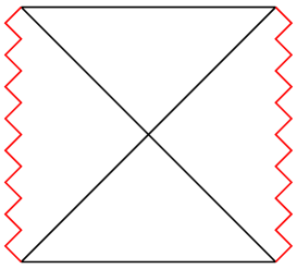
Figure 9: The conformal diagram for negative $\mu$.

Another simple extension of the solutions given in eq. (36) comes from introducing a ‘charged black hole’ into dS space. The corresponding metric may be written as

$$ds^{2}=-\frac{1}{H(\rho)}d\rho^{2}+H(\rho)d\tau^{2}+\frac{\rho^{2}}{\ell^{2}}d\Sigma^{2}_{k,n-1}\ ,$$ (41)

where

$$H(\rho)=\frac{\rho^{2}}{\ell^{2}}-k+\frac{\mu}{\rho^{n-2}}+\frac{Q^{2}}{\rho^{2n-4}},$$ (42)

and our notation is adapted to the asymptotic cosmological regions where the ‘radial’ variable $\rho$ appears timelike. Of course, the full solution now contains a Maxwell field and the electrostatic potential will have the form: $\phi(\rho)\propto Q/\rho^{n-2}$. For $k=+1$, this reproduces the standard Reissner-Nordstrom-dS solution.

Of course if $Q=0$, eq. (41) provides a vacuum solution and for $k=+1$, this reproduces the standard Schwarzschild-dS solution. For these vacuum solutions with $\mu$ positive, $k=+1$ is the only case for which there may be cosmological (and black hole) event horizons. For $k=0,-1$, the solutions have a spacelike or cosmological singularity at $\rho=0$. If $\mu$ is negative, all of the solutions have a cosmological horizon which separates the asymptotically dS regions from timelike singularities at $\rho=0$, as illustrated in figure 9. The connection of these solutions to the dS/CFT duality were discussed in, e.g., ref. [10, 11]. Similar comments apply about the causal structure for the full solution with $Q\not=0$.

Interpreted as a renormalization group flow, this family of solutions (41) is interesting as the scaling of the $\tau$ direction is different from that for the remaining boundary directions. However, for the vacuum solutions with $Q=0$, the corresponding flows are trivial in that the c-function (27) is simply a fixed constant since $\Lambda_{eff}=\Lambda$. On the other hand, with the background Maxwell field (i.e., $Q\not=0$), we have a time-dependent $\Lambda_{eff}$. The c-function (27) for the flow under consideration has the form

$$c\sim\Lambda_{eff}^{-(n-1)/2}=\left|G^{\rho}{}_{\rho}\right|^{-(n-1)/2}\ .$$ (43)

From eq. (41), we find

$$\Lambda_{eff}=-G^{\rho}{}_{\rho}=\frac{n(n-1)}{2\ell^{2}}-\frac{(n-1)(n-2)Q^{2}}{2\rho^{2(n-1)}}\ .$$ (44)

Eq. (44) is a monotonically increasing function from $\rho\rightarrow+\infty$. It is finite both on $I^{-}$ and at the cosmological horizon $\rho=\rho_{+}$, which is the largest root for $H(\rho_{+})=0$. We find that for all possible values of $n$, $Q$ and $k$, the c-function (27) is monotonically decreasing from $I^{-}$ to the cosmological horizon at $\rho=\rho_{+}$. Hence this provides a nontrivial example of our c-theorem of section 4.

Appendix B Numerical bouncing universe

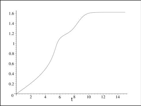
Figure 10: The scalar field $\phi(t)$ increases steadily until it reaches its maximum value at the wall of the potential where it becomes frozen.

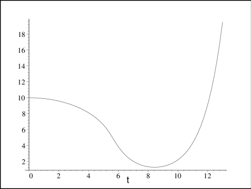
Figure 11: The behavior of the scale factor is such that the universe contracts from $t=0$ up to when the scalar field hits the wall of the potential. Then the universe re-enters an expansion phase. The equations of motion are symmetric when $t\rightarrow-t$ so the model of universe presented is in fact asymptotically dS on $I^{\pm}$.

In section 6, we constructed an asymptotically dS solution with a very large matter-dominated region in the middle. The potential used there was rather unrealistic (i.e., discontinuous). To assure the skeptical reader that our results are not an artifact of this construction, we present an analogous numerical solution here using an everywhere smooth potential. While smooth, however, the potential has edges which can be made arbitrarily sharp,

$$V(\phi)=\frac{1}{2L^{2}}\frac{\tanh w(\phi-\phi_{0})-\tanh w(\phi+\phi_{0})+2\tanh w\phi_{0}}{\tanh w\phi_{0}}.$$ (45)

The parameter $w$ characterizes the steepness of the potential steps and $\pm\phi_{0}$ are approximately the values of the scalar field where the jumps occur. This potential is chosen to be symmetric in $\phi\rightarrow-\phi$, so that we may consider a time symmetric solution. Further the potential is constructed such that $L$ corresponds to the cosmological scale in the asymptotic regions. That is, $\Lambda_{final}=3/L^{2}$ as we are working in four dimensions ($n=3$) in the following.

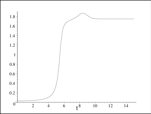
Figure 12: The effective cosmological for the numerical bouncing universe is such that the spacetime is asymptotically de Sitter in the future.

Solving the second order Friedmann equation (15) numerically using Maple yields the scalar field and a scale factor respectively shown on figures 10 and 11 given we use the initial conditions

$$\ a(0)=1,\ \ \phi(0)=0,\ \ \dot{a}(0)=0,\ \ {\rm and}\ \ \dot{\phi}(0)=10.$$ (46)

The parameters in eq. (45) are chosen such that $w=10$, $\phi_{0}=1$ and

$$L=\alpha\frac{a(0)^{3}\dot{\phi}(0)}{\cosh^{\frac{3}{2}}(2\phi(0))}.$$ (47)

The final parameter $\alpha$ was tuned to study various different classes of solutions. For $\alpha=1$, the value of $L$ given by eq. (47) corresponds to the maximum potential step which the scalar could climb with the given initial conditions, according the construction of section 3.2. The figures illustrate various aspects of the evolution for $\alpha=.9558$. The equations of motion being left unchanged when $t\rightarrow-t$, the flow from $t=-\infty$ to $t=0$ can be deduced simply by using the reflection of figures 10 and 11 across the $t=0$ axis. Figure 12 shows the evolution of the effective cosmological constant $\Lambda_{eff}$. Note that asymptotically $\Lambda_{eff}$ is a constant (as is the scalar) indicating that the evolution reaches an asymptotically dS phase. Hence the full solution would begin in a dS phase, then enter a matter (scalar) dominated bounce and finally return to a dS phase, just as described for the ‘very tall’ universe models in section 6.

From examining figures 11 and 12, we see that $\Lambda_{eff}$ increases monotonically during the contracting phase of the evolution and decreases in the expanding phase, in accord with the c-theorem of section 4. It is interesting to note that for $\alpha>.9559$ (holding all other parameters fixed) the scalar continues to roll after climbing up the wall and the resulting kinetic energy forces the scale factor to contract into a big crunch. On the other hand, for $\alpha<.9557$ (again holding all other parameters fixed) the field fails to completely climb the wall and $\phi$ returns to zero, again resulting in a big crunch. Only in the (approximate) range $.9557<\alpha<.9559$ do the solutions reach an asymptotically de Sitter regime.

Figure 13: Conventions for the $R,T,U$ coordinates.

Appendix C Conformal diagram of $k=0$ de Sitter flows

In this appendix we finish the derivation of figure 5 (b), the conformal diagram for asymptotically de Sitter spaces with flat spatial slices. As described in section 4, the diagram will consist of two regions, each of which is conformal to one quadrant of Minkowski space and each of which has an interior that is foliated by flat spatial hypersurfaces. One of these regions may be represented by a quadrant of a diamond as shown in figure 4 (b), but this fixes part of the conformal freedom so that the representation of the second region is more constrained. To find its shape it is useful to choose explicit coordinates. Let us begin by introducing the null coordinates $u=\tau-r$ and $v=\tau+r$ and the corresponding $U=\tanh(u)$, $V=\tanh(v)$. We shall also introduce $T,R$ by $U=T-R$ and $V=T+R$ and take the convention that our conformal diagrams are drawn in such a way that $T,R$ appear as Cartesian coordinates. In particular, we take the boundaries of the triangle in figure 13 to lie at $T=0$, $R=0$, and $U=-1.$

Note that we retain the conformal freedom to replace $U$ by any smooth function of $U$ in the region $U<-1$. We may therefore use this freedom to place $I^{-}$ on some convenient line, subject only to the constraint that the angle (in the Lorentzian geometry sense) between $I^{-}$ and $R=0$ is unchanged. A convenient choice is to use the analogue of a constant $t$ line in the region beyond $U=-1$. That is, we define a new coordinate $u^{\prime}(U)=\tanh(2+U)$ in this region and use a line of the form $u^{\prime}+v=T_{0}$.

It remains only to determine the location of the left timelike boundary of our diagram, which will represent the center of spherical symmetry for the flat slices beyond our Cauchy horizon. Note that this line must intersect each surface of homogeneity orthogonally. Thus, the shape of this boundary will be determined if we find the surfaces of homogeneity.

Figure 14: The form of the line representing $I^{-}$.

To do so, we simply extend the coordinate $r$ to range over $[-\infty,\infty]$ on both sides of the Cauchy horizon. This corresponds to taking a slice all of the way across our original higher dimensional spacetime instead of truncating the slice at $r=0$. For any such slice there is a translation that reduces to $\frac{\partial}{\partial r}$ along the slice, so that we may consider $\frac{\partial}{\partial r}$ to generate surfaces of homogeneity in the above spacetime. The important point is that, since $\frac{\partial}{\partial r}$ is a Killing field of the spacetime, it must be a conformal Killing field of the conformally re-scaled spacetime drawn in the diagram above. As a result, it must be of the form $f(U)\frac{\partial}{\partial U}+g(v)\frac{\partial}{\partial v}$ across the entire conformal diagram.

Now, in the upper triangle, the expression for $\frac{\partial}{\partial r}$ in terms of $\frac{\partial}{\partial U}$ and $\frac{\partial}{\partial v}$ is fixed and can be computed from the coordinate definitions. The same function $g(v)$ must therefore give the component of $\frac{\partial}{\partial r}$ along $\frac{\partial}{\partial v}$ in the lower part of the diagram. It remains only to determine the function $f(U)$ giving the component along $\frac{\partial}{\partial U}$ for $U<-1.$ But this is fixed by the requirement that $I^{-}$ be along the line $u+v=T_{0}$. Since $I^{-}$ is a surface of homogeneity, $\frac{\partial}{\partial r}$ must be tangent to $\frac{\partial}{\partial u}-\frac{\partial}{\partial v}$ at $T=-1$. This suffices to determine $f(U)$ for $U<-1$. Without solving these equations in detail, it is clear that the result is simply that the left timelike boundary is a line of the form $u-v=R_{0}$.

Figure 15: The coordinate $r$ is extended to range over the real line.

If one desires, one can perform a transformation (a translation in $u$ and $v$) to the conformal frame shown below in which the diagram has a $Z_{2}$ symmetry of inversion through the center. Again, focusing arguments imply that the figure must be ‘taller than it is wide,’ so that the dashed congruence of light rays in figure 16 does not pass from $I^{-}$ to $I^{+}$.

Figure 16: The diagram for an asymptotically de Sitter spacetime with flat surfaces of homogeneity in a) the frame described above and b) a frame where the diagram has a reflection symmetry though the center.

References

-
[1]
S. Perlmutter et al. [Supernova Cosmology Project Collaboration],
“Measurements of the Cosmological Parameters and from the First
Seven Supernovae at z0.35,”
Astrophys. J. 483, 565 (1997) [arXiv:astro-ph/9608192];
S. Perlmutter et al. [Supernova Cosmology Project Collaboration], “Discovery of a Supernova Explosion at Half the Age of the Universe and its Cosmological Implications,” Nature 391, 51 (1998) [arXiv:astro-ph/9712212];
A.G. Riess et al. [Supernova Search Team Collaboration], “Observational Evidence from Supernovae for an Accelerating Universe and a Cosmological Constant,” Astron. J. 116, 1009 (1998) [arXiv:astro-ph/9805201].;
N.A. Bahcall, J.P. Ostriker, S. Perlmutter and P.J. Steinhardt, “The Cosmic Triangle: Revealing the State of the Universe,” Science 284, 1481 (1999) [arXiv:astro-ph/9906463]. - [2] A. Strominger, “The dS/CFT correspondence,” JHEP 0110, 034 (2001) [arXiv:hep-th/0106113].
- [3] A. Strominger, “Inflation and the dS/CFT correspondence,” JHEP 0111, 049 (2001) [arXiv:hep-th/0110087].
- [4] V. Balasubramanian, J. de Boer, and D. Minic, “Mass, Entropy, and Holography in Asymptotically de Sitter spaces” [arXiv:hep-th/0110108].
- [5] E. Witten, “Quantum gravity in de Sitter space,” arXiv:hep-th/0106109.
- [6] R. Bousso, A. Maloney and A. Strominger, “Conformal vacua and entropy in de Sitter space,” arXiv:hep-th/0112218.
- [7] M. Spradlin and A. Volovich, “Vacuum states and the S-matrix in dS/CFT,” arXiv:hep-th/0112223.
- [8] T. Banks, “Cosmological breaking of supersymmetry or little Lambda goes back to the future II,” [arXiv:hep-th/0007146].
- [9] V. Balasubramanian, P. Horava, and D. Minic, “Deconstructing De Sitter,” JHEP 0105, 043 (2001) [arXiv:hep-th/0103171].
- [10] A.M. Ghezelbash and R.B. Mann, “Action, mass and entropy of Schwarzschild-de Sitter black holes and the de Sitter/CFT correspondence,” JHEP 0201, 005 (2002) [arXiv:hep-th/0111217].
- [11] R.G. Cai, Y.S. Myung and Y.Z. Zhang, “Check of the mass bound conjecture in de Sitter space,” arXiv:hep-th/0110234.
-
[12]
D. Klemm,
“Some aspects of the de Sitter/CFT correspondence,”
Nucl. Phys. B 625, 295 (2002)
[arXiv:hep-th/0106247];
S. Cacciatori and D. Klemm, “The asymptotic dynamics of de Sitter gravity in three dimensions,” Class. Quant. Grav. 19, 579 (2002) [arXiv:hep-th/0110031]. - [13] M. Li and F.L. Lin, “Note on holographic RG flow in string cosmology,” arXiv:hep-th/0111201.
- [14] S. Gao and R. M. Wald, “The physical process version of the first law and the generalized second law for charged and rotating black holes,” Phys. Rev. D 64, 084020 (2001) [arXiv:gr-qc/0106071].
- [15] R. Wald, General Relativity (U. of Chicago, 1984).
- [16] R. Bousso, “Positive vacuum energy and the N-bound,” JHEP 0011, 038 (2000) [arXiv:hep-th/0010252].
- [17] R. Bousso, O. DeWolfe and R.C. Myers, in preparation.
- [18] See, for example: S.W. Hawking and G.F.R. Ellis, The large scale structure of space-time (Cambridge: Cambridge University Press, 1980).
- [19] O. DeWolfe, D.Z. Freedman, S.S. Gubser and A. Karch, “Modeling the fifth dimension with scalars and gravity,” Phys. Rev. D 62, 046008 (2000) [hep-th/9909134]; K. Skenderis and P.K. Townsend, “Gravitational stability and renormalization-group flow,” Phys. Lett. B 468, 46 (1999) [arXiv:hep-th/9909070].
- [20] O. Aharony, S.S. Gubser, J. Maldacena, H. Ooguri and Y. Oz, “Large N field theories, string theory and gravity,” Phys. Rept. 323,183 (2000) [arXiv:hep-th/9905111].
- [21] L. Susskind and E. Witten, “The holographic bound in anti-de Sitter space,” arXiv:hep-th/9805114.
- [22] A.W. Peet and J. Polchinski, “UV/IR relations in AdS dynamics,” Phys. Rev. D 59, 065011 (1999) [arXiv:hep-th/9809022].
-
[23]
J. Distler and F. Zamora,
“Non-supersymmetric conformal field theories from stable anti-de Sitter spaces,”
Adv. Theor. Math. Phys. 2, 1405 (1999) [arXiv:hep-th/9810206];
L. Girardello, M. Petrini, M. Porrati and A. Zaffaroni, “Novel local CFT and exact results on perturbations of N=4 super Yang-Mills from AdS dynamics,” JHEP 9812, 022 (1998) [arXiv:hep-th/9810126];
D.Z. Freedman, S.S. Gubser, K. Pilch and N.P. Warner, “Continuous distributions of D3-branes and gauged supergravity,” JHEP 0007, 038 (2000) [arXiv:hep-th/9906194];
N.R. Constable and R.C. Myers, “Exotic scalar states in the AdS/CFT correspondence,” JHEP 9911, 020 (1999) [arXiv:hep-th/9905081];
L. Girardello, M. Petrini, M. Porrati and A. Zaffaroni, “The supergravity dual of N = 1 super Yang-Mills theory,” Nucl. Phys. B 569, 451 (2000) [arXiv:hep-th/9909047]. - [24] A.B. Zamolodchikov, “Irreversibility of the Flux of the Renormalization Group in a 2D Field Theory,” JETP Lett. 43, 730 (1986) [Pisma Zh. Eksp. Teor. Fiz. 43, 565 (1986)].
- [25] D.Z. Freedman, S.S. Gubser, K. Pilch and N.P. Warner, “Renormalization group flows from holography supersymmetry and a c-theorem,” Adv. Theor. Math. Phys. 3, 363 (1999) [arXiv:hep-th/9904017].
-
[26]
J. de Boer, E. Verlinde and H. Verlinde,
“On the holographic renormalization group,”
JHEP 0008, 003 (2000) [arXiv:hep-th/9912012];
V. Balasubramanian, E.G. Gimon and D. Minic, “Consistency conditions for holographic duality,” JHEP 0005, 014 (2000) [arXiv:hep-th/0003147];
V. Sahakian, “Holography, a covariant c-function and the geometry of the renormalization group,” Phys. Rev. D 62, 126011 (2000) [arXiv:hep-th/9910099];
E. Alvarez and C. Gomez, “Geometric holography, the renormalization group and the c-theorem,” Nucl. Phys. B 541, 441 (1999) [arXiv:hep-th/9807226]. - [27] R. Emparan, C. V. Johnson and R. C. Myers, “Surface terms as counterterms in the AdS/CFT correspondence,” Phys. Rev. D 60, 104001 (1999) [arXiv:hep-th/9903238].
- [28] J. Louko and D. Marolf, “Single-exterior black holes and the AdS-CFT conjecture,” Phys. Rev. D 59, 066002 (1999) [arXiv:hep-th/9808081].
- [29] J.M. Maldacena, “Eternal black holes in Anti-de-Sitter,” [arXiv:hep-th/0106112].
- [30] A. Borde and A. Vilenkin, “Eternal Inflation And The Initial Singularity,” Phys. Rev. Lett. 72, 3305 (1994) [arXiv:gr-qc/9312022].
- [31] A. Borde and A. Vilenkin, “The Impossibility Of Steady State Inflation,” arXiv:gr-qc/9403004.
- [32] A. Borde and A. Vilenkin, “Singularities in inflationary cosmology: A review,” Int. J. Mod. Phys. D 5, 813 (1996) [arXiv:gr-qc/9612036].
- [33] A. Borde, A. H. Guth and A. Vilenkin, “Inflation is not past-eternal,” arXiv:gr-qc/0110012.
- [34] T. Vachaspati and M. Trodden, Phys. Rev. D 61, 023502 (2000) [arXiv:gr-qc/9811037].
- [35] B. McInnes, “The dS/CFT correspondence and the big smash,” arXiv:hep-th/0112066.
- [36] R. Bousso, “Holography in general space-times,” JHEP 9906, 028 (1999) [arXiv:hep-th/9906022]; “A Covariant Entropy Conjecture,” JHEP 9907, 004 (1999) [arXiv:hep-th/9905177].
- [37] E. Flanagan, D. Marolf, and R. Wald, “Proof of Classical Versions of the Bousso Entropy Bound and of the Generalized Second Law,” Phys. Rev. D 62, 084035 (2000) [arXiv:hep-th/9908070].
- [38] J.M. Maldacena and L. Susskind, “D-branes and Fat Black Holes,” Nucl. Phys. B 475, 679 (1996) [arXiv:hep-th/9604042].
- [39] G.T. Horowitz and T. Jacobson, “Note on gauge theories on M/ and the AdS/CFT correspondence,” JHEP 0201, 013 (2002) [arXiv:hep-th/0112131].
- [40] L. Susskind, L. Thorlacius and J. Uglum, “The Stretched horizon and black hole complementarity,” Phys. Rev. D 48, 3743 (1993) [arXiv:hep-th/9306069].
- [41] L. Susskind, “String theory and the principles of black hole complementarity,” Phys. Rev. Lett. 71, 2367 (1993) [arXiv:hep-th/9307168].
- [42] L. Susskind and L. Thorlacius, “Gedanken experiments involving black holes,” Phys. Rev. D 49, 966 (1994) [arXiv:hep-th/9308100].
- [43] F. Leblond, D. Marolf and R.C. Myers, “Tall tales from de Sitter space II,” in preparation.