The Splitting of Branes on Orientifold Planes

Abstract:

Continuing the study in hep-th/0004092, we investigate a non-trivial string dynamical process related to orientifold planes, i.e., the splitting of physical NS-branes and $D(p+2)$-branes on orientifold $Op$-planes. Creation or annihilation of physical $Dp$-branes usually accompanies the splitting process. In the particular case $p=4$, we use Seiberg-Witten curves as an independent method to check the results.

1 Introduction

The brane setup [1] (for a review, see [2]) has been proved to be a very useful tool to relate string theory to field theory. On one hand, we can use known results in string theory to get non-trivial new results in field theory. For instance, mirror symmetry in three dimensions [3] can be easily studied by brane setup [1, 4, 5, 6, 7, 8]. On the other hand, field theory considerations can be used to predict non-trivial dynamics in string theory. One of the most known examples is the generation or annihilation of a $D3$-brane when a $D5$-brane crosses an NS-brane [1]. This prediction and its generalizations were demonstrated later from various points of view [9, 10, 11, 12, 13, 14, 15, 16].

In this note, we want to study one prediction about string dynamics which was found in [8] using consistency arguments within field theory. In [8], in order to construct mirror pairs by $O3$-planes, two of us made a conjecture on the splitting of a physical brane (NS-brane and $D5$-brane) on the $O3$-planes. The general picture of splitting is given in Figure 1. Initially, a 1/2NS-brane with non-vanishing $X^{789}$ is separated from its image (see part (a)). Then, we move them towards the orientifold plane at $X^{789}=0$. When they touch the orientifold, they are on top of each other. Since now each piece is mirror to itself, they can move along the $X^{6}$-direction independently (see part (b)). This process is called “splitting”.

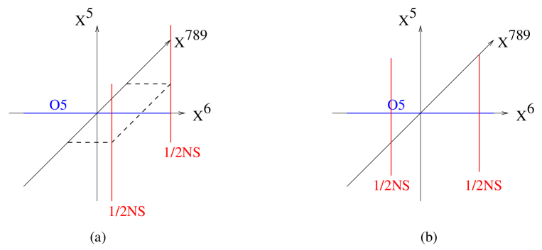
Figure 1: (a) 1/2NS-brane and its image have the same $X^{6}$ coordinate. (b) After splitting, they have different $X^{6}$ coordinates.

The results of splitting in [8] are as follows. A physical $D5$-brane splits without the generation of branes on the $O3^{+},O3^{-},\widetilde{O3^{+}}$ planes, while a physical $D3$-brane is generated on the $\widetilde{O3^{-}}$-plane. The splitting of a physical NS-brane can be derived from the $D5$-brane case by S-duality. The NS-brane will split freely, namely without the generation of branes, on $\widetilde{O3^{-}},O3^{-},\widetilde{O3^{+}}$ planes, while a physical $D3$-brane is generated on the $O3^{+}$ plane.

We got the above results indirectly by using field theory arguments. It would be very interesting to gather more evidence to support them, or even derive them directly. Furthermore, it would be very nice to discuss how NS-branes and $D(p+2)$-branes split on $Op$-planes for arbitrary $p$. It turns out that the splitting of $D(p+2)$-branes on $Op$-planes is universal for $p\leq 6$, namely the conclusions we have derived for the case of $D5$-branes on O3-planes hold for all $p$. However, the splitting of NS-branes on $Op$-planes is more complex and there is no universal behavior. Each case has to be discussed separately. The results can be summarized in the following table:

Type $$p=1$$

(1)

In the table above, $1$ means that a $Dp$-brane is generated while $-1$ means that a $Dp$-brane is annihilated. For the annihilation to be possible, we need enough $Dp$-branes on top of the orientifold before the splitting. The $M$ for the $p=6$ case is the cosmological constant which we will discuss in more detail later. For $p=5$ case, the $\leq 2$ means that any number of branes which is less than or equal to two is allowed (we use the convention that a negative number means annihilation).

The above conclusions are derived by several consistency arguments. In the special case of $p=4$, we can check the result by studying the Coulomb branch of ${\cal N}=2$ symplectic and orthogonal gauge theories realized in this brane setup. In particular, we will analyze the corresponding Seiberg-Witten curves.

The plan of the paper is as follows. In section 2, we derive the general splitting rules for both $D$-branes and NS-branes. In section 3, we explain how to check these rules in the specific case of the NS-brane splitting on $O4$-planes by Seiberg-Witten curves. Then, we introduce the curves for ${\cal N}=2$ theories with a single symplectic or orthogonal gauge group. In section 4, we write down the curves for a product of symplectic and orthogonal gauge groups and then study the NS-brane splitting.

2 The general picture of the splitting

In this section, we will give the general picture of the splitting of physical $D$-branes and NS-branes on $Op$-planes. We will argue that the splitting of $D$-branes on orientifolds is universal, while the splitting of NS-branes is not.

The plan for this section is as follows. In section 2.1, we study the universal splitting of $D$-branes. In section 2.2, we observe that for NS-branes, the splitting is not universal so that we need to discuss each case separately. In section 2.3, we use the minimum energy argument to derive the splitting of NS-branes on $Op$-planes with $p\leq 4$. In section 2.4 and 2.5, we use proper consistency conditions, i.e., the cosmological constant argument for $p=6$ and charge conservation for $p=5$, to reach the desired results.

2.1 The universal splitting of $D$-branes

First, let us discuss the splitting of a physical $D(p+2)$-brane on $Op^{\pm},\widetilde{Op^{\pm}}$-planes for $p\leq 6$ . The $D(p+2)$-brane is extended along the $X^{012\ldots(p-1)}$ and $X^{789}$ directions, while the $Op$-plane is extended along the $X^{012\ldots(p-1)}$ and $X^{6}$ directions . There are actually more than four kinds of $O1$-planes, but we will not discuss all of them in this paper and refer the reader to [17, 18, 19]. We will give several arguments to show that the splitting of a physical $D(p+2)$-brane on $Op$-planes is universal: the $D(p+2)$-brane will split freely on $Op^{+},Op^{-},\widetilde{Op^{+}}$ planes, while a physical $Dp$-brane is created on the $\widetilde{Op^{-}}$-plane .

The first argument, which was employed in [8], involves the Higgs mechanism. Let us consider the familiar brane setup given by two 1/2NS-branes, $k$ physical $Dp$-branes and $n$ physical $D(p+2)$-branes which preserves 8 supercharges. The $Dp$-branes are parallel to the $Op$-plane and the 1/2NS-branes are extended along the $X^{012345}$ directions. Depending on the type of $Op$-planes, we have different $p$-dimensional gauge theories: $Sp(k)$ for $Op^{+}$, $Sp^{\prime}(k)$ for $\widetilde{Op^{+}}$, $SO(2k)$ for $Op^{-}$ and $SO(2k+1)$ for $\widetilde{Op^{-}}$. All of them have $n$ hypermultiplets, except for $Sp^{\prime}(k)$ gauge theory which has two extra half-hypermultiplets. We can Higgs the above theories down to, for example, $Sp(k-1),Sp(k-1),SO(2k-1)$ and $SO(2k)$ by breaking one physical $Dp$-brane between the NS-branes and the $D(p+2)$-branes. Now we need to match the degrees of freedom before and after Higgsing. From the field theory point of view, when we Higgs the gauge theory, one vector multiplet always eats one hypermultiplet. This is true in any dimension, because there are 8 supercharges . So, after Higgsing, we get the lower rank gauge theories, some hypermultiplets in the fundamental representation and some hypermultiplets in the singlet representation. From the brane setup point of view, the Higgsing simply corresponds to the breaking of $Dp$-branes between 1/2NS-branes and 1/2$D(p+2)$-branes. Matching the degrees of freedom that can be read from the brane setup with field theory, we find the results given at the end of the last paragraph.

To make the above argument more transparent, let us consider one example, i.e., the splitting of a $D(p+2)$-brane on the $\widetilde{Op^{-}}$-plane. The brane setup is given in Figure 2. The gauge theory is $SO(2k+1)$ with $N$ hypermultiplets (see part (a)). After splitting the $D(p+2)$-brane, a $Dp$-brane is generated as in part (b). Then we move the 1/2$D(p+2)$-branes across the two 1/2NS-branes. From part (c), we see that the remaining theory is $SO(2k)$ with $N-1$ hypermultiplets and $N$ singlets . Notice that the $Dp$-brane generated by the splitting of the $D(p+2)$-brane does not contribute any vector multiplet. Now, let us count the various degrees of freedom. Before Higgsing, we have $N(2k+1)=2kN+N$ degrees of freedom. After Higgsing, we have $(N-1)2k+N=2kN+N-2k$ only. However, taking into account the $k(2k+1)-k(2k-1)=2k$ degrees of freedom which have been eaten by the vector multiplets, the two numbers match exactly, $2kN+N-2k+2k=2kN+N$. The same argument can be applied to other cases.

Figure 2: (a) The brane setup of the gauge theory. (b) The splitting of a $D(p+2)$-brane on the $\widetilde{Op^{-}}$-plane with the generation of one $Dp$-brane. (c) The final theory after Higgsing.

The second argument is based on T-duality. Let us give an example, namely the derivation of the splitting of a $D6$-brane on $\widetilde{O4^{-}}$, to illustrate the idea. We start from the known result of the splitting of a $D5$-brane on $\widetilde{O3^{-}}$. First, we compactify the $X^{3}$ direction and get two fixed $O3$-planes which are shown in part (a) of Fig. 3. It is important to notice that the two $1/2D5$-branes intersect only the upper $O3$-plane. Notice also that, in order to get $\widetilde{O4^{-}}$ after T-duality, we set the lower $O3$-plane to be $O3^{-}$. After T-duality, $\widetilde{O3^{-}}$ and $O3^{-}$ combine to give $\widetilde{O4^{-}}$, while $O3^{-}$ and $O3^{-}$ combine to give an $O4^{-}$, as in part (b). ¿From part (b), we can read off that a physical $D4$-brane is generated when a physical $D6$-brane splits on $\widetilde{O4^{-}}$. We can also reach part (b) by splitting one $D5$-brane on the lower $O3^{-}$-plane, as shown in part (c). Since two $\widetilde{O3^{-}}$-planes yield one $O4^{-}$ with one physical $D4$-brane, we obtain the same result.

The T-duality argument can be easily generalized to other cases. One will find the universal behavior we claimed before. For instance, we can compactify the $X^{2}$ direction instead of the $X^{3}$ direction to find the splitting of a $D4$-brane on $O2$-planes. In this case, it is important to recall the result of [19] that, after T-duality, the $O3$-plane will be divided into two $O2$-planes, but the $1/2D4$-branes will intersect only one $O2$-plane.

Figure 3: Part (a) shows that a $D3$-brane is generated when a $D5$-brane splits on the upper $\widetilde{O3^{-}}$-plane. Part (b) is T-dual to Part (a). (c) Instead of splitting on the upper plane, we split the $D5$-brane on the lower $O3^{-}$ plane. No $D3$-branes appear and after T-duality we recover Part (b) again.

There are other universal behaviours, like the bending of the branes and the charge difference of the orientifold planes on the two sides of a 1/2$D(p+2)$-brane. They will be addressed in next subsection when we discuss the splitting of NS-branes.

All of this evidence supports the claim that the splitting of $D(p+2)$-branes on $Op$-planes is universal.

2.2 The non-universal behaviour of the NS-brane splitting

Now let us discuss the splitting of physical NS-branes on $Op$-planes. One may think that we can solve this problem by T-duality, but there are actually several observations that indicate the failure of naive T-duality. For example, it is well known that a $D4$-brane is created after an NS-brane crosses a $D6$-brane. But after T-duality, there is no brane creation after a Kaluza-Klein monopole crosses a $D5$-brane, as shown in [20].

Let us recall that the NS-branes are extended along the $X^{012345}$ directions and that the $Op$-plane is extended along the $X^{012\ldots(p-1)}$ and $X^{6}$ directions.

First of all, let us consider the bending of an NS-brane due to the intersection with $Dp$-branes. From Witten’s work [21], such a bending can be found approximately by solving

$$\bigtriangledown^{2}x^{6}=q\delta^{(6-p)}(r-r_{0})$$ (2)

where function $x^{6}(r)$ represents the bending of the NS-brane along the $X^{6}$ direction, $q$ is the $D$-brane charge deposited at the intersection points $r_{0}$ and $\bigtriangledown^{2}$ is the Laplacian operator in the NS-brane worldvolume coordinates. Far away from the $Op$-plane, the bending of $x^{6}$ goes like $r^{p-4}$. So, when $p\leq 3$, the bending caused by the intersection will disappear at large distance, while when $p=4,5$ the bending will propagate to infinity. This transition from $p=3$ to $p=4$ is the first sign that we should be careful while applying T-duality.

Let us compare the above bending of NS-branes with the one of $D(p+2)$-branes. Since a $D(p+2)$-brane always has three non-compact transverse dimensions relative to the Dp-brane, its bending goes like $r^{-1}$ and disappears at infinity, which does not depend on $p$. This difference between the non-universal bending of NS-branes and the universal bending of $D(p+2)$-branes indicates why T-duality is applicable to the $D$-brane system but not to the NS-brane system.

The second observation is related to the charge difference between the two $Op$-planes on the two sides of the intersection. On one hand, at the intersection with a 1/2NS-brane, the charge difference is $2\times 2^{p-5}=2^{p-4}$ for the $Op^{\pm}$ pair and $2^{p-5}-(\frac{1}{2}-2^{p-5})=2^{p-4}-\frac{1}{2}$ for the $\widetilde{Op^{\pm}}$ pair, both depending on $p$. On the other hand, at the intersection with a 1/2$D(p+2)$-brane, the charge difference is always $\frac{1}{2}$ for the $Op^{-},\widetilde{Op^{-}}$ pair and zero for $Op^{+},\widetilde{Op^{+}}$ pair, no matter what $p$ is.

The third observation concerns the different behaviour of NS-branes and $D$-branes under T-duality. If we T-dualize one dimension down, we get two fixed $O(p-1)$-planes. A 1/2NS-brane will intersect both fixed planes, while a $1/2D(p+1)$-brane (the T-dual of a $1/2D(p+2)$-brane) will intersect only one of these two fixed planes. These different intersection properties have very important consequences. For example, if T-duality is correct, the $D3$-brane generated on the $O3^{+}$-plane by splitting the NS-brane should be divided into two equal parts on both $O2^{+}$-planes, i.e. there is a $1/2D2$-brane generated when an NS-brane splits on an $O2^{+}$-plane, which is not allowed. If we went further, we would come up with the conclusion that there is a quarter physical $D1$-brane generated when an NS-brane splits on an $O1^{+}$-plane. This is obviously wrong. In the $D$-brane case, we do not have this problem because the $D$-branes will intersect with and split on only one of these two fixed planes, hence we do not need to divide the effect into two parts.

On these grounds, it is clear we should rely on other methods to discuss the splitting of NS-branes on $Op$-planes. In the case of $O3$-planes, we can apply S-duality. For $p\leq 4$, we can use a minimum energy argument. For $p=5$, we need to analyze the relative $(p,q)$-web. For $p=6$, the configuration has to be consistent with RR charge conservation in a background with a possibly non-vanishing cosmological constant. The details of these methods are given in the following subsections.

2.3 The minimum energy argument

There are two sources of energy costs when we try to split a physical brane into two half branes (two 1/2$D(p+2)$-branes or 1/2NS-branes) on the $Op$-plane. The first one is the energy it takes to bend a 1/2$D(p+2)$-brane or 1/2NS-brane. The bending energy is proportional to the absolute value of the $Dp$-brane charge difference between the two sides. The second one is due to the creation (which costs energy) or annihilation (which produces energy) of $Dp$-branes, parallel to the $Op$-plane, between the two 1/2-branes. The minimum configuration is the balance between these two factors. For $p\leq 4$, since the 1/2NS-brane has more transverse directions than the $Dp$-branes, the energy cost from the first source dominates. For $p=5,6$ the second source becomes important so we need to be more careful. However, in this subsection, we focus on the $p\leq 4$ case only.

2.3.1 The $D(p+2)$-brane case

To check that our minimum energy argument is right, we apply it to the splitting of $D(p+2)$-branes. Since $D(p+2)$-branes have two transverse directions more than $Dp$-branes, the first source is more important. The charge difference between the two sides of the split 1/2$D(p+2)$-brane is given by the following table

Type $$\Delta q$$   for  D(p+2)

where $N$ is the number of $Dp$-branes generated in the middle when we split the $D(p+2)$-brane. Note that there is no dependence on $p$, signalling a universal behaviour for $D(p+2)$-branes. Thus we see that, in order to minimize the energy cost, we need to choose $N=0$ in the first two cases, $N=0,-1$ in the third case and $N=0,1$ in the last case.

We need a complementary argument to fix the ambiguity in the last two cases. This is provided by field theory as we discussed above. Namely, we need to match the Higgs branch before and after the Higgsing mechanism.

The above discussion is applied to all $p\leq 6$, and in particular also to the $\widetilde{O6^{-}}$-plane, whose existence was argued by [22]. Note that, upon crossing a 1/2NS-brane, the $\widetilde{O6^{-}}$-plane becomes a $\widetilde{O6^{+}}$-plane [23, 24], which indicates the existence of the $\widetilde{O6^{+}}$-plane. Furthermore, since $O6^{\pm}$-planes can exist in a background with vanishing cosmological constant, they can also exist with an arbitrary integer cosmological constant. This is due to the fact that, by crossing an arbitrary number of physical $D8$-planes, the $O6^{\pm}$-planes remain such while the cosmological constant jumps by an integer. Conversely, since we have found that a physical $D8$-brane can split into two 1/2$D8$-branes, we see that the $\widetilde{O6^{\pm}}$-planes can exist in a background with arbitrary half-integer cosmological constant [22]. This observation will be important later when we discuss the splitting of NS-branes.

2.3.2 The NS-brane case

Now we calculate the bending energy of a 1/2NS-brane, which for $p\leq 4$ is proportional to the $Dp$-brane charge difference between the two sides, which is given by

Type $$\Delta q$$   for  NS

where $N$ is the number of $Dp$-branes generated in the middle when we split the NS-brane. Note that the result depends on $p$, giving evidence of non-universal behavior. The number $N$ corresponding to the minimum energy cost is listed below

Type $$p=1$$

(3)

Except for $p=1,2$, the minimum energy requirement does not fix the number uniquely. We need to discuss each case separately. For $p=3$, S-duality tells us that $N=1$ for $O3^{+}$ and $N=0$ for $O3^{-}$.

For $p=4$, we need to take into account that the bending is like $\ln r$, so that when two 1/2NS-branes bend towards each other, they will finally meet and combine to give a physical NS-brane which is not bent. To see it clearly, let us discuss the example of $\widetilde{O4^{+}}$. If we choose $N=1$ for $\widetilde{O4^{+}}$, the distance between these two 1/2NS-branes will become infinite as we move away from the intersection point with the $O4$-plane (see part (a) of Figure 4). Such a bending will cost an infinite amount of energy, and we can rule it out. On the other hand, if we choose $N=0$ for $\widetilde{O4^{+}}$, these two 1/2NS-branes will meet each other (see part (b) Figure 4) and combine to give an NS-brane. This configuration definitely costs less energy, so we should choose $N=0$. By the same argument, we have that $N=-1$ for the case $\widetilde{O4^{-}}$.

Figure 4: The bending of 1/2NS-branes after splitting on the $\widetilde{O4^{+}}$-plane for case (a) $N=1$ and (b) $N=0$.

2.4 The splitting of NS-branes on $O6$-planes

When we consider the NS/$D6$-brane system, we need to take the cosmological constant $M$ into account [25, 26]. In this background, RR charge conservation requires that

$$N_{L}-N_{R}=M\,,$$

where $N_{L}$ is the number of $D6$-branes ending on the left hand side of the NS-brane and $N_{R}$ is the number of $D6$-branes ending on the right hand side. In the presence of an orientifold, the same formula holds for a 1/2NS-brane with the understanding that $N_{L},N_{R}$ are the D6-brane charges.

The general framework for our discussion is depicted in Figure 5. In part (a), we have $N_{L}$ and $N_{R}$ $1/2D6$-branes ending on the two sides of two 1/2NS-branes and the consistency condition reads

$$1/2(N_{L}-N_{R})=M\,.$$

After the splitting, we have $2N_{L}$ $1/2D6$-branes ending on the left, $2N_{R}$ $1/2D6$-branes ending on the right and $2N$ $1/2D6$-branes in the middle (see part (b)). The consistency conditions become

$$[(N_{L}+q_{1})-(N+q_{2})]=M,~{}~{}~{}~{}~{}~{}~{}~{}~{}~{}[(N+q_{2})-(N_{R}+q_{1})]=M$$

where $q_{1},q_{2}$ are the charges of the left (or right) and middle orientifold planes respectively. Notice that these two conditions imply that $1/2(N_{L}-N_{R})=M$, which is consistent with part (a). Now we can solve these two equations and get

$$N_{L}-N=M+q_{2}-q_{1}$$

Putting different $q_{1},q_{2}$, we can summarize the results in the following table

$q_{1}$ charge	$O6^{+}$	$O6^{-}$	$\widetilde{O6^{+}}$	$\widetilde{O6^{-}}$
$N$	$N_{L}-(M-4)$	$N_{L}-(M+4)$	$N_{L}-(M-7/2)$	$N_{L}-(M+7/2)$

Note that since $N_{L},N$ and $N_{R}$ are integers, the cosmological constant $M$ has to be an integer in the $O6^{\pm}$ case and half-integer in the $\widetilde{O6^{\pm}}$ case for the splitting to be possible . This condition on $M$ is perfectly consistent with our observation at the end of section $2.1$.

Figure 5: The splitting of an NS-brane on $O6$-planes with cosmological constant $M$. (a) Before the splitting, we have $1/2(N_{L}-N_{R})=M$. (b) After the splitting, $N$ physical (or $2N$ half) $D6$-branes are generated.

2.5 The splitting of NS-branes on $O5$-planes

In this case, things become more interesting. We not only have NS-branes or D5-branes, but also general $(p,q)$-branes with $p,q$ coprime[27, 28]. Charge conservation at the intersection point becomes the necessary condition for the configuration to be consistent. Supersymmetry further requires the orientation of branes to be fixed by their $(p,q)$-charges and the string coupling constant $g_{s}$.

Let us recall some facts about the general $(p,q)$-web. Define

$$\tau=\xi/2\pi+i/\lambda\,.$$ (4)

The tension of a $(p,q)$-brane is

$$T_{p,q}=|p+\tau q|T_{D5}\,,$$ (5)

(from this we see that $(1,0)$ is a $D5$-brane and $(0,1)$ is an NS-brane. This is the convention used in the paper). To preserve a quarter of the original supersymmetry, the orientation of the $(p,q)$-brane is given by

$$\Delta x+i\Delta y||p+\tau q\,.$$ (6)

When we include $O5$-planes along the $x$-direction, to be consistent with the $Z_{2}$ orientifold action, $\tau$ must be a pure imaginary number, namely $\xi=0$. If we use this condition, we will have that

$$T_{p,q}=T_{D5}\sqrt{p^{2}+|\tau q|^{2}}$$ (7)

with the orientation

$$\Delta x/\Delta y=p/(-i\tau q)$$ (8)

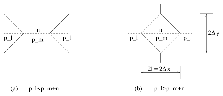
Figure 6: The setup of NS-brane splitting on $O5$-planes, where $p_{l},p_{m}$ are the charges of the orientifolds on the l.h.s. (the same as r.h.s.) and in the middle and $n$ is the number of $D5$-branes generated in the splitting process. (a) the bending when $p_{l}<p_{m}+n$. (b) the bending when $p_{l}>p_{m}+n$. In this case, the 1/1-branes meet and combine to become one physical NS-brane again.

Now we can start the calculation of the energy cost. The general setup is given in Figure 6. When $p_{l}<p_{m}+n$, the brane bending is like in part (a) which will cost an infinite amount of energy. This leaves us the condition that $p_{l}\geq p_{m}+n$. For $p_{l}=p_{m}+n$ with integer $n$, the brane does not bend and the energy cost is

$$2lnT_{D5}+2l(p_{m}-p_{l})T_{D5}=0$$

where the first term is the contribution from the generated D5-branes (remember that negative $n$ means annihilation) and the second term is the contribution from the change of orientifold plane. Next, consider the case $p_{l}>p_{m}+n$ as in part (b) of Figure 6. Charge conservation tells us that the bent branes are $((p_{l}-(p_{m}+n))/2,\pm 1/2)$-branes. From it we get

$$|\Delta y| = |(\tau l)/(p_{l}-(p_{m}+n))|,$$

$$length = \sqrt{l^{2}+(\Delta y)^{2}}=l\sqrt{1+(\frac{|\tau|}{p_{l}-p_{m}-n})^{2}},$$

$$E_{bending} = 4T_{p,q}length=lT_{D5}2(p_{l}-p_{m}-n)[1+(\frac{|\tau|}{p_{l}-p_{m}-n})^{2}]$$

Now the change of energy is

$$\Delta E = 2lnT_{D5}+2l(p_{m}-p_{l})T_{D5}+E_{bending}-2T_{D5}|\tau|\frac{|\tau|l}{p_{l}-p_{m}-n}$$

$$= 0$$

where in the first line, the third term (the bending energy) minus the fourth term (the original non-bending part of the NS-brane) give the energy cost for the bending.

From this calculation we see that as long as $p_{l}\geq p_{m}+n$, any $n$ is a good choice since all of them cost the same energy ($zero$). It seems to be a little surprising. However, notice that we can relate configurations of different $n$ by a smooth motion with $zero$ energy cost, so that above results make perfect sense. Now inserting the proper values of $p_{l},p_{m}$, we can find the results shown in the table in the introduction. For example, putting $p_{l}=+1$ ($O5^{+}$) and $p_{l}=-1$ ($O5^{-}$) we get $n\leq 2$.

There are several points we want to discuss. First, we notice that the change of total energy after splitting on $O5$-planes is $zero$. Does this hold for other $Op$-planes? It does not seem so. In general situations, the total energy of the system does not change before and after the splitting, but sometimes it does. For example, when an NS-brane splits on an $O3^{-}$-plane, there is no brane created or annihilated, but the 1/2NS-brane does bend. In other words, in the splitting process we do put energy into the system.

The change of total energy may cause some confusion because it seems that during the whole process the system is supersymmetric and the motion is smooth. In fact, if two parallel branes are static, they do preserve half the amount of initial supersymmetry, but if they move relatively to each other, all supersymmetries are broken. The splitting process, no matter how slow it is, does break supersymmetry, so we cannot use the supersymmetry argument to require that the energy is the same before and after splitting. To make this point more clear, let us recall the following brane setup given in [1]: $N$ D3-branes ending on two parallel NS-branes. If we keep the positions of the D3-branes on the NS-branes invariant and push these two NS-branes away from each other, the bending of the NS-branes will be same, but the length of the D3-branes will increase, which means that the total energy of the brane system does increase.

The second point we want to discuss is that for the $\widetilde{O5^{\pm}}$ cases, we have D-brane charge $(p_{l}-p_{m}-n)/2=\pm 3/4-n/2$ for the bending brane if we demand the charge conservation condition at the intersection point. The appearance of a quarter charge D-brane is a non-trivial prediction by splitting process. However, the legitimacy of a quarter charge D-brane is not very clear to us at this moment. We have several arguments to support its existence, but we still cannot draw a definite conclusion from them. First, if we do not allow for a quarter charge D-brane, we would violate charge conservation at the intersection point and the energy change before and after splitting would not be zero. The second point is that the D-brane with quarter charge is not complete. It sits at $X^{789}=0$, like the orientifold plane, and must be accompanied by its image. If we draw them in real space (not the covering space in Figure 6), they are on top of each other. So, when we calculate the D5-brane charge, we must sum them together and we get a half-integer charge which would not violate the Dirac quantization condition. In comparison, a 1/2D5-brane and its image can have nonzero $X^{789}$, so when we draw them in real space, they are not on top of each other and the D-brane charge is not the sum. The third point is that branes with quarter charge and their images can never be on top of the orientifold because, if they were, they would change the type of orientifold and cause an inconsistency. The last point is that a 1/2NS-brane does exist on $\widetilde{O5^{\pm}}$-planes. This can be seen from the following brane construction given in Figure 7. In part (a), there are two physical D5-branes ending on the r.h.s. of a 1/2NS-brane. Then, we move the 1/2D7-brane to the right and reach part (b). Since part (a) exists, part (b) must exist too.

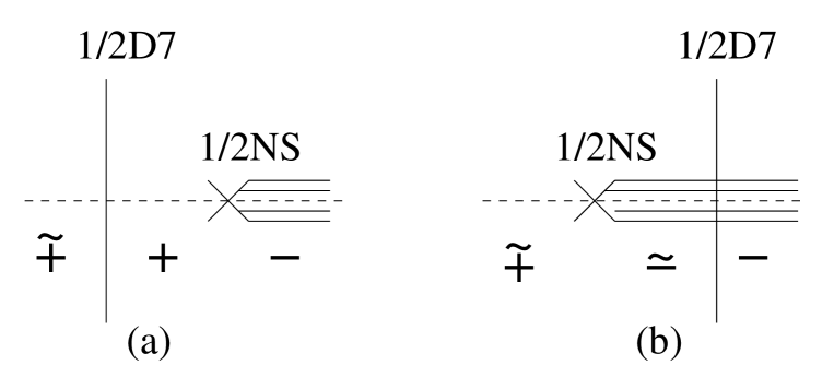
Figure 7: The proof that a 1/2NS-brane does exist on $\widetilde{O5^{\pm}}$-planes. Starting from part (a), which we know is an allowed configuration, by moving the 1/2D7-brane to the right, we reach part (b), where the 1/2NS-brane intersects the $\widetilde{O5^{\pm}}$-plane.

3 Analysis of $p=4$ by Seiberg-Witten curves

We get the splitting rules in general situations by using various arguments. However, it would be very satisfactory if we had some more direct way to derive them. Although we do not know how to do this for general $p$, in the case of $O4$-planes, we can check the above results by studying the Coulomb branch of symplectic and orthogonal gauge theories arising on the worldvolume of $D4$-branes stretched between the 1/2NS-branes.

The general idea is the following. Let us start from the brane setup with $N$ physical $D4$-branes on top of $O4$-planes and some physical NS-branes above the $O4$-planes (see, for example, part (a) of Figure 8). Then, we move the NS-branes to touch the $O4$-planes and split them into 1/2NS-branes, where we assume this is allowed. Next, we split the $D4$-branes and let them end on the 1/2NS-branes. After these operations, we get various gauge theories between the 1/2NS-branes with rank $N^{\prime}$ and $N$. As we know $N^{\prime}$ can differ from $N$. As a matter of fact, this is exactly the brane configuration considered in [29] to derive the Seiberg-Witten curves for the Coulomb branch of ${\cal N}=2$ symplectic and orthogonal gauge theories via M-theory, generalizing the work of Witten for the Coulomb branch of ${\cal N}=2$ $SU(N)$ gauge theories [21] (see part (b) of Figure 8).

If the above splitting process is correct, we can reverse it. Namely, we can move two 1/2NS-branes towards each other and combine them into one physical NS-brane which can then leave the $O4$-plane.

The low-energy physics in the Coulomb branch is encoded in a polynomial with non trivial dependence on the moduli and scales of the various theories, the Seiberg-Witten curve. If the reverse process is possible, the Seiberg-Witten curve undergoes a specific factorization. In the following, we are going to study the conditions for this transition to happen.

We have to remark that this analysis via the Coulomb branch is not general, in the sense that the gauge theories between the 1/2NS-branes have to be asymptotically free or conformal. This imposes certain conditions on the number of $D4$-branes ending on the various 1/2NS-branes. The condition has a simple geometrical picture. Since the inverse Yang-Mills coupling, $1/g^{2}_{YM}$, is proportional to the distance between the 1/2NS-branes, in the AF case the distance between them increases as we move away from the $O4$-plane and the $D4$-branes, whereas the distance remains invariant in the conformal case [21, 29].

3.1 The general setup

Before delving into a detailed discussion in the next section, let us set up the general framework to investigate the splitting of the NS-brane.

We are going to consider only four 1/2NS-branes with $D4$-branes stretched between them, as in part (c) of Figure 8. In particular, there are no $D4$-branes on the l.h.s of A2 nor on the r.h.s. of C1. This configuration corresponds to a product of three gauge theories with a certain number of flavors for each factor: the type of $O4$-plane between two 1/2NS-branes dictates the gauge group on the $D4$-branes worldvolume. Recall that after crossing a 1/2NS-brane the minus charged $O4$-planes are changed into plus charged $O4$-planes and vice versa: for example, $O4^{+}$ turns into $O4^{-}$ and $\widetilde{O4^{-}}$ turns into $\widetilde{O4^{+}}$ [23, 24]. In the following table we list the various gauge group factors from left to right and the number of flavors for each factor depending on the type of $O4$-plane between A2 and B1,

Type Gauge groups Number of Flavors

$$O4^{+}$$

(9)

A careful analysis of the Seiberg-Witten curve will tell us if one can move the two middle 1/2NS-branes on top of each other by properly adjusting the gauge theory moduli and scales. Conversely, if this is possible, a physical NS-brane can be split on the corresponding $O4$-plane.

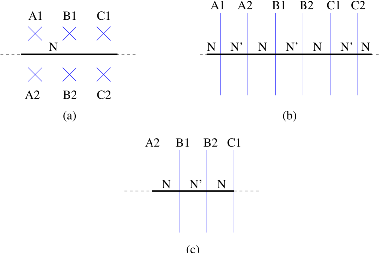
Figure 8: (a) Three physical NS-branes before the splitting. (a) The gauge field theories constructed by the splitting of NS-branes and $D4$-branes. (c) Our framework of gauge field theories.

3.2 The Seiberg-Witten curve of a single gauge group with flavors

The results for the ${\cal N}=2$ $SU(2)$ gauge theory obtained in the celebrated papers [30, 31] have since been generalized to other gauge groups : to $SU(n)$ groups in [32, 33, 34, 35], to $SO(2k)$ in [36, 37], to $SO(2k+1)$ in [37, 38] and to $Sp(k)$ in [39, 40]. In this paper, we will follow the conventions of [39].

3.3 The Seiberg-Witten curves for $SO$ and $Sp$ groups

The Seiberg-Witten curves for $Sp(r)$, $SO(2r)$ and $SO(2r+1)$ are given in [39]. The coefficients of the $\beta$-functions are

$$b_{Sp}=2r+2-N_{f},~{}~{}~{}~{}~{}b_{SO}=N_{c}-2-N_{f}~{}~{}.$$

So when $N_{f}=2r+2$ for $Sp(r)$, $N_{f}=2r-2$ for $SO(2r)$ and $N_{f}=2r-1$ for $SO(2r+1)$, the theories are conformal. It is understood that the following results apply to asymptotically free theories only.

The corresponding curves are summarized in the table

$$Sp(r)$$

(10)

where

$$g(\tau)=\frac{\vartheta_{2}^{4}(\tau)}{\vartheta_{3}^{4}(\tau)+\vartheta_{4}^{4}(\tau)},~{}~{}~{}~{}~{}f(\tau)=\frac{\vartheta_{2}^{4}(\tau)\vartheta_{4}^{4}(\tau)}{(\vartheta_{2}^{4}(\tau)-\vartheta_{4}^{4}(\tau))^{2}}~{}\,,$$ (11)

and

$$\tau=\frac{\theta}{\pi}+i\frac{8\pi}{g^{2}}$$

As we explain in the appendix, following [35] and [39], $f(\tau+1)$ and $g(\tau+1)$ actually yield physically equivalent curves. Matching the brane picture will fix the modular function: we will encounter this feature when we discuss the splitting of NS-branes. Note that sending $\tau$ to $\tau+1$ amounts to shifting $\theta$ by $\pi$.

The Jacobi theta functions are defined by

$$\begin{array}[]{rclrcl}\vartheta_{2}(\tau)&=&\sum_{n\in Z}q^{(n+\frac{1}{2})^{2}},{}{}{}{}{}{}{}&\vartheta_{2}^{4}&=&16q+O(q^{3}),\\ &&&&&\\ \vartheta_{3}(\tau)&=&\sum_{n\in Z}q^{n^{2}},&\vartheta_{3}^{4}&=&1+8q+O(q^{2}),\\ &&&&&\\ \vartheta_{4}(\tau)&=&\sum_{n\in Z}(-1)^{n}q^{n^{2}},&\vartheta_{4}^{4}&=&1-8q+O(q^{2}),\end{array}$$ (12)

$$q\equiv e^{i\pi\tau}=e^{i\pi(\frac{\theta}{\pi}+i\frac{8\pi}{g^{2}})}=e^{i\theta}e^{-8\pi^{2}/g^{2}}\,,$$

and they satisfy the Jacobi identity

$$\vartheta_{2}^{4}(\tau)-\vartheta_{3}^{4}(\tau)+\vartheta_{4}^{4}(\tau)=0\,.$$

Furthermore, in the limit $q\rightarrow 0$,

$$g(\tau)\rightarrow 8q,~{}~{}~{}~{}f(\tau)\rightarrow 16q$$

To get the curve for the asymptotically free theories with $N_{f}$ flavors, for example $N_{f}<2r+2$ for the $Sp(r)$ group, we take $2r+2-N_{f}$ masses to be equal to $M$ and then send $M$ to $\infty$ while keeping $\Lambda^{2r+2-N_{f}}=\Lambda^{b_{Sp}}=qM^{2r+2-N_{f}}$ finite (so $q\rightarrow 0$ in such limit). By such an operation we get the curve

$$Sp(r)$$

(13)

3.4 The corresponding curves from M-theory

The corresponding curves of the above gauge groups, i.e. $Sp(r)$, $SO(2r)$ and $SO(2r+1)$ are derived via M-theory in [29]. For later purposes, we are interested in finding the explicit dependence of the various curve parameters on the dynamical scales.

The curves of single gauge groups in [29] can be summarized as

$$Sp(r)$$

(14)

where $B(v^{2})$ is a polynomial in $v^{2}$ with degree $r$ and $e,c,f,h$ are constants which may be functions of the flavour masses $m_{i}$ and the dynamical scale $\Lambda$. Furthermore, the constant $c$ is fixed by requiring the curve to have a double root at $v^{2}=0$ [29].

Comparing table (14) with (13), it is easy to find the correspondence

group non-conformal conformal

$$Sp(r)$$

(15)

where we list the results both for the conformal and the non-conformal case.

3.5 The $Sp^{\prime}(r)$ gauge group

$Sp^{\prime}(r)$ gauge theory is a little mysterious and there is no direct result from the field theory point of view. However, from the brane setup, it is very natural to write down the Seiberg-Witten curve. Loosely speaking, $Sp^{\prime}(r)$ with $N_{f}$ flavors is equivalent to $Sp(r)$ with $N_{f}+1$ flavors, one of which is massless. Using this correspondence, we can heuristically derive the curve for $Sp^{\prime}(r)$. First, let us recall the $Sp(r)$ case, whose curve is given by

$$\prod_{i=1}^{N_{f}^{L}}(v^{2}-m_{i}^{2})t^{2}+e(v^{2}B(v^{2})+8\Lambda^{b_{Sp}}\prod_{i=1}^{N_{f}}m_{i})t+\frac{e^{2}}{4}(-1)^{b_{Sp}}64\Lambda^{2b_{Sp}}\prod_{j=1}^{N_{f}^{R}}(v^{2}-m_{j}^{2})=0.$$

To connect with the $Sp^{\prime}(r)$ case, we multiply by $v$ both the $t^{2}$ term and the $t^{0}$ term. This is because the massless half-hypermutiplet corresponds to $\sqrt{v^{2}-m^{2}}=v$. Since we have added two half-hypermultiplets, the number of flavors changes from $N_{f}$ to $N_{f}+1$, which implies $b_{Sp}\rightarrow b_{Sp^{\prime}}=2r+2-(N_{f}+1)$. Furthermore,

$$8\Lambda^{2r+2-N_{f}}\prod_{i=1}^{N_{f}}m_{i}\longrightarrow 8\Lambda^{2r+2-N_{f}-1}\prod_{i=1}^{N_{f}+1}m_{i}=0$$

because $m_{N_{f}+1}=0$. Combining all these facts together we find the curve

$$v\prod_{i=1}^{N_{f}^{L}}(v^{2}-m_{i}^{2})t^{2}+ev^{2}B(v^{2})t+\frac{e^{2}}{4}(-1)^{b_{Sp^{\prime}}}64\Lambda^{2b_{Sp^{\prime}}}v\prod_{j=1}^{N_{f}^{R}}(v^{2}-m_{j}^{2})=0$$ (16)

with $N_{f}^{L}+N_{f}^{R}=N_{f}$. We can factor out one $v$ and get

$$\prod_{i=1}^{N_{f}^{L}}(v^{2}-m_{i}^{2})t^{2}+evB(v^{2})t+\frac{e^{2}}{4}(-1)^{b_{Sp^{\prime}}}64\Lambda^{2b_{Sp^{\prime}}}\prod_{j=1}^{N_{f}^{R}}(v^{2}-m_{j}^{2})=0$$ (17)

In the conformal case, the curve is

$$\prod_{i=1}^{N_{f}^{L}}(v^{2}-m_{i}^{2})t^{2}+evB(v^{2})t+\frac{e^{2}}{4}g^{2}(\tau)\prod_{j=1}^{N_{f}^{R}}(v^{2}-m_{j}^{2})=0$$ (18)

4 The Splitting of the NS-brane

After this introduction, it is time to test the results on the splitting of NS-branes on $O4$-planes using the Seiberg-Witten curves. Our general framework is depicted in figure 8. We will first write down the Seiberg-Witten curves for three gauge groups, including their dynamical scales, and then check if the curves allow the splitting. We define $v=X^{4}+iX^{5}$, $s=(X^{6}+iX^{10})/R$ (where $R$ is the radius of compact $X^{10}$ direction), and $t=e^{-s}$ as in [21][29].

4.1 The curve of $Sp(k_{1})\times SO(2k_{2})\times Sp(k_{3})$

The beta-function coefficients are

$$b_{Sp_{1}}=2k_{1}+2-k_{2},~{}~{}~{}~{}~{}b_{SO_{2}}=2k_{2}-2-(k_{1}+k_{3}).~{}~{}~{}~{}~{}b_{Sp_{3}}=2k_{3}+2-k_{2},$$

The curve without dynamical scales is given in [29] by

$$t^{4}+(v^{2}B_{1}(v^{2})+C)t^{3}+B_{2}(v^{2})t^{2}+(v^{2}B_{3}(v^{2})+D)t+1=0\,.$$

In order to find the explicit dependence on them, we follow the method used in [41]. If we assign the value $2k_{1}+2$ to the dimension of $t$, then every term in the curve has dimension $8k_{1}+8$. So, we propose the following curve

$$t^{4}+(v^{2}B_{1}(v^{2})+C)t^{3}+c_{1}\Lambda_{1}^{2b_{Sp_{1}}}B_{2}(v^{2})t^{2}+c_{2}\Lambda_{1}^{4b_{Sp_{1}}}\Lambda_{2}^{2b_{SO_{2}}}(v^{2}B_{3}(v^{2})+D)t+$$

$$c_{3}\Lambda_{1}^{6b_{Sp_{1}}}\Lambda_{2}^{4b_{SO_{2}}}\Lambda_{3}^{2b_{Sp_{3}}}=0$$ (19)

The constants $C,D$ are determined by requiring that the curve (19) has double roots at $v=0$ [29]. After some algebra, we find

$$\begin{array}[]{rcl}C&=&\sqrt{4c_{1}\Lambda_{1}^{2b_{Sp_{1}}}B_{2}(0)-8(x\sqrt{c_{3}})\Lambda_{1}^{3b_{Sp_{1}}}\Lambda_{2}^{2b_{SO_{2}}}\Lambda_{3}^{b_{Sp_{3}}}},\\ &&\\ D&=&C\frac{x\sqrt{c_{3}}}{c_{2}}\Lambda_{1}^{-b_{Sp_{1}}}\Lambda_{3}^{b_{Sp_{3}}}\,,\end{array}$$ (20)

where $x$ can be $\pm 1$.

After fixing $C$ and $D$, we solve for the constants $c_{1},c_{2},c_{3}$ by taking various decoupling limits of (19) and matching the result with the curves for single gauge groups. For example, sending first $\Lambda_{3}$ to zero and then $\Lambda_{2}$, we decouple the gauge groups $SO(2k_{2})$ and $Sp(k_{3})$, and we are left with the curve

$$t^{2}+(v^{2}B_{1}(v^{2})+C^{\prime})t+c_{1}(\Lambda_{1}^{2b_{Sp_{1}}})B_{2}(v^{2})=0\,.$$

Matching the above with the curve of $Sp(k_{1})$ in Table 14, we find

$$c_{1}=16(-1)^{b_{Sp_{1}}}.$$

It is a little tricky to determine the constant $c_{2}$. Again, we decouple $Sp(k_{3})$ by letting $\Lambda_{3}\rightarrow 0$. This yields

$$t^{3}+(v^{2}B_{1}(v^{2})+C)t^{2}+c_{1}\Lambda_{1}^{2b_{Sp_{1}}}B_{2}(v^{2})t+c_{2}\Lambda_{1}^{4b_{Sp_{1}}}\Lambda_{2}^{2b_{SO_{2}}}(v^{2}B_{3}(v^{2})+D)=0.$$

To decouple $Sp(k_{1})$, we need to rescale $t$ first. Substituting $t$ with $t\Lambda_{1}^{2b_{Sp_{1}}}$ in the above equation, cancelling the common factor $\Lambda_{1}^{4b_{Sp_{1}}}$ and then letting $\Lambda_{1}\rightarrow 0$, we finally come to

$$(v^{2}B_{1}(v^{2})+C)t^{2}+c_{1}B_{2}(v^{2})t+c_{2}(\Lambda_{2}^{2b_{SO_{2}}})(v^{2}B_{3}(v^{2})+D)=0$$

In this limit, we also have $C=0,D=0$. Matching with the $SO(2k_{2})$ curve in Table 14, we find

$$c_{2}=16c_{1}^{2}(-)^{b_{SO_{2}}+1}=16^{3}(-)^{b_{SO_{2}}+1}$$

Repeating the procedure once again, we find

$$\frac{c_{3}}{c_{1}}=16\left(\frac{c_{2}}{c_{1}}\right)^{2}(-1)^{b_{Sp_{3}}},~{}~{}~{}~{}~{}D^{\prime}=8\Lambda_{3}^{b_{Sp_{3}}}\sqrt{(-1)^{k_{2}}B_{2}(0)}\,.$$

Therefore

$$c_{1}=16(-1)^{b_{Sp_{1}}},~{}~{}~{}~{}~{}c_{2}=16^{3}(-1)^{b_{SO_{2}}+1},~{}~{}~{}~{}~{}~{}c_{3}=16^{6}(-1)^{b_{Sp_{3}}}=16^{6}(-1)^{b_{Sp_{1}}+b_{Sp_{3}}}\,,$$ (21)

and $x=(-1)^{b_{SO_{2}}+1}$.

Note that the curve (19) is symmetric under the transformation $t\rightarrow t$ and $v\rightarrow-v$. This is a consequence of the orientifold action, which reads $X^{6,10}\rightarrow X^{6,10}$ and $X^{4,5}\rightarrow-X^{4,5}$ and is equivalent to the above transformations of $t$ and $v$ [29].

If $b_{SO_{2}}=0$, the curve is obtained from the above by replacing $16(-1)^{b_{SO_{2}}}\Lambda_{2}^{2b_{SO_{2}}}$ with $f(\tau_{2})$, where $f(\tau_{2})$ is given in (11),

$$t^{4}+(v^{2}B_{1}(v^{2})+C)t^{3}+16(-1)^{b_{sp1}}\Lambda_{1}^{2b_{Sp_{1}}}B_{2}(v^{2})t^{2}$$

$$-2^{8}\Lambda_{1}^{4b_{Sp_{1}}}f(\tau_{2})(v^{2}B_{3}(v^{2})+C\Lambda_{1}^{-b_{Sp_{1}}}\Lambda_{3}^{b_{Sp_{3}}})t+2^{16}\Lambda_{1}^{6b_{Sp_{1}}}f(\tau_{2})^{2}\Lambda_{3}^{2b_{Sp_{3}}}=0,$$ (22)

and

$$C=8\Lambda_{1}^{b_{Sp_{1}}}\sqrt{(-1)^{b_{Sp_{1}}}B_{2}(0)+2^{5}\Lambda_{1}^{b_{Sp_{1}}}f(\tau_{2})\Lambda_{3}^{b_{Sp_{3}}}}\,.$$ (23)

4.2 Lifting of the middle 1/2NS-branes

Our goal is to understand which conditions the curve (19) must satisfy in order to be able to lift the middle 1/2NS-branes, B1 and B2, out of the orientifold plane (see part (c) of figure 8). The remaining configuration, with A2 and C1 only, would describe a single symplectic gauge group theory.

First of all, if we want to move the two 1/2NS-branes B1 and B2 out of the orientifold plane, we have to reconnect the $D4$-branes to the left of B1 with the $D4$-branes to the right of B2. In particular, the two symplectic gauge groups at both ends of the configuration must have the same rank. Thus, we will set $k_{1}=k_{3}$ in (19), which leads to $b_{Sp_{1}}=b_{Sp_{3}}\equiv b_{Sp}$.

Furthermore, since in this case the left and right gauge theory are the same, we can write the curve in a more symmetric form which is invariant under the exchange of the left and right gauge groups. Recalling that $X^{6}$ and $X^{10}$ are the coordinates along the orientifold plane, the above requirement amounts to the curve (19) being symmetric under $X^{6,10}\to-X^{6,10}$, after setting the origin of these coordinates appropriately. This transformation is equivalent to $t\to 1/t$.

This gives a relation between $B_{1}(v^{2})$ and $B_{3}(v^{2})$ in (19). Setting $\Lambda_{1}=\Lambda_{3}\equiv\Lambda$, and performing the rescaling $t\rightarrow i2^{6}\Lambda^{2b_{Sp}}\Lambda_{2}^{b_{SO_{2}}}t\equiv At$, the curve becomes

$${\cal P}(v^{2},t)\equiv A^{4}t^{4}+(v^{2}B_{1}(v^{2})+C)A^{3}t^{3}+c_{1}\Lambda^{2b_{Sp}}B_{2}(v^{2})A^{2}t^{2}+(v^{2}B_{3}(v^{2})+C)A^{3}t+A^{4}=0$$ (24)

where we have used the fact that $C=D$ by (20). Finally, we see that, in order to achieve the $t\to 1/t$ symmetry,

$$t^{4}{\cal P}(v^{2},1/t)={\cal P}(v^{2},t)\,,$$ (25)

$B_{1}(v^{2})$ must be equal to $B_{3}(v^{2})$.

At a certain stage in the lifting procedure, the middle NS5-branes will coincide. We want to argue that in this limit

$${\cal P}(v^{2},t)\rightarrow{\cal R}(t){\cal Q}(v^{2},t),$$ (26)

where ${\cal R}(t)$ is a quadratic polynomial in $t$ with a double root and ${\cal Q}(v^{2},t)$ is another quadratic polynomial in $t$ with some $v$ dependence describing an $Sp(r)$ theory with no flavours. Recall from [21] and [29] that the roots in $t$ of ${\cal P}(v^{2},t)$ at a given $v$ correspond to the positions of the NS5-branes in the $t$-plane. Requiring no $v$ dependence and a double root for ${\cal R}(t)$ precisely depicts the situation where the middle NS5-branes are on top of each other. Furthermore, we can manipulate (14) so that ${\cal Q}(v^{2},t)$ itself will have a $t\to 1/t$ symmetry

$$t^{2}{\cal Q}(v^{2},1/t)={\cal Q}(v^{2},t)\,.$$

We are now going to show that for the case at hand, namely when the middle orthogonal theory is not conformal, the splitting procedure is not possible.

First of all, let us find ${\cal R}(t)$. Then, Eqs. (25) and (26) imply that

$$t^{4}{\cal R}(1/t){\cal R}^{-1}(t)={\cal Q}(v^{2},t){\cal Q}(v^{2},1/t)^{-1}={\cal Q}(0,t){\cal Q}(0,1/t)^{-1}=t^{2},$$

which fixes ${\cal R}(t)$ to be proportional to $(t+x)^{2}$, where $x=\pm 1$. Setting

$${\cal P}(v^{2},t)=(t+x)^{2}\left(2^{8}\Lambda_{1}^{2b_{Sp_{1}}}\Lambda_{2}^{2b_{SO_{2}}}t^{2}+(e^{2}v^{2}\tilde{B}(v^{2})+\beta)t+2^{8}\Lambda_{1}^{2b_{Sp_{1}}}\Lambda_{2}^{2b_{SO_{2}}}\right)=0,$$

we derive the following relations

$$-4i\Lambda_{2}^{b_{SO_{2}}}(v^{2}B_{1}(v^{2})+C)=e^{2}v^{2}\tilde{B}(v^{2})+\beta\,,$$

$$(-1)^{b_{Sp_{1}}+1}B_{2}(v^{2})=2x(e^{2}v^{2}\tilde{B}(v^{2})+\beta)+2^{9}\Lambda_{1}^{2b_{Sp_{1}}}\Lambda_{2}^{2b_{SO_{2}}}\,.$$

In particular

$$(-1)^{b_{Sp_{1}}+1}B_{2}(v^{2})-2^{9}\Lambda_{1}^{2b_{Sp_{1}}}\Lambda_{2}^{2b_{SO_{2}}}=-8xi\Lambda_{2}^{b_{SO_{2}}}(v^{2}B_{1}(v^{2})+C)\,,$$

implying that, in the non trivial case, namely when $\Lambda_{2}^{b_{SO_{2}}}$ does not vanish, $v^{2}B_{1}(v^{2})$ and $B_{2}(v^{2})$ must have the same order. But this is equivalent to $k_{1}+1=k_{2}$ or $b_{SO_{2}}=0$. Therefore, we conclude that the lifting cannot happen when the middle orthogonal theory is not conformal.

Let us turn to the curve (15) describing the conformal case. If we set $f(\tau_{2})=-\alpha^{2}$, with $\alpha$ to be determined, and perform a redefinition of $t$, $t\to 2^{4}\Lambda_{1}^{2b_{Sp_{1}}}\alpha\,t$, the curve becomes

$$2^{12}\Lambda_{1}^{6b_{Sp_{1}}}\alpha^{2}\left(2^{4}\alpha^{2}\Lambda_{1}^{2b_{Sp_{1}}}t^{4}+\alpha(v^{2}B_{1}(v^{2})+C)t^{3}+\right.$$

$$\left.(-1)^{b_{sp1}}B_{2}(v^{2})t^{2}+\alpha(v^{2}B_{1}(v^{2})+C)t+2^{4}\alpha^{2}\Lambda_{1}^{2b_{Sp_{1}}}\right)=0.$$

In this form, the curve has a $t\to 1/t$ symmetry. In the limit where the middle NS5-branes coincide, this should be equal to

$$2^{12}\Lambda_{1}^{6b_{Sp_{1}}}\alpha^{2}(t+x)^{2}\left(2^{4}\Lambda_{1}^{2b_{Sp_{1}}}\alpha^{2}t^{2}+(e^{2}v^{2}\tilde{B}(v^{2})+\beta)t+2^{4}\Lambda_{1}^{2b_{Sp_{1}}}\alpha^{2}\right)=0,$$

where $x=\pm 1$. This equation yields

$$\alpha(v^{2}B_{1}(v^{2})+C)=e^{2}v^{2}\tilde{B}(v^{2})+\beta+2^{5}x\alpha^{2}\Lambda_{1}^{2b_{Sp_{1}}}\,,$$ (27)

and

$$(-1)^{b_{Sp_{1}}}B_{2}(v^{2})=2xe^{2}v^{2}\tilde{B}(v^{2})+2x\beta+2^{5}\alpha^{2}\Lambda_{1}^{2b_{Sp_{1}}}\,.$$ (28)

Therefore

$$(-1)^{b_{Sp_{1}}}B_{2}(v^{2})=2x\alpha(v^{2}B_{1}(v^{2})+C)-2^{5}\alpha^{2}\Lambda_{1}^{2b_{Sp_{1}}}\,.$$ (29)

Since the highest order coefficients both in $B_{1}(v^{2})$ and $B_{2}(v^{2})$ are $1$, the above equation implies that $\alpha={(-1)^{b_{Sp_{1}}}\over 2}x$ and

$$f(\tau_{2})=-{1\over 4}.$$ (30)

Furthermore, using (23), where we set $\Lambda_{1}^{b_{Sp_{1}}}=\Lambda_{3}^{b_{Sp_{3}}}$, (27) and (28), we get that

$$\alpha C=2^{6}x\alpha^{2}\Lambda_{1}^{b_{Sp_{1}}},\quad\beta=2^{5}x\alpha^{2}\Lambda_{1}^{b_{Sp_{1}}}\,.$$

The remaining symplectic theory is then described by the curve

$$2^{4}\alpha^{2}(\Lambda_{1}^{2b_{Sp_{1}}})t^{2}+\alpha(v^{2}B_{1}(v^{2})+2^{5}x\alpha\Lambda_{1}^{2b_{Sp_{1}}})t+2^{4}\alpha^{2}(\Lambda_{1}^{2b_{Sp_{1}}})=0,$$ (31)

to be compared with

$$t^{2}+e(v^{2}\tilde{B}(v^{2})+8\Lambda^{b_{Sp}})t+16e^{2}\Lambda^{2b_{sp}}=0.$$

Note that $b_{Sp}=2k_{1}+2=2b_{Sp_{1}}=2(2k_{1}+2-k_{2})=2(k_{1}+1)$. By setting $2^{2}\alpha\Lambda_{1}^{b_{Sp_{1}}}t\to t$, (31) becomes

$$t^{2}+{1\over 4}\Lambda_{1}^{-b_{Sp_{1}}}(v^{2}B_{1}(v^{2})+2^{5}x\alpha\Lambda_{1}^{2b_{Sp_{1}}})t+2^{4}\alpha^{2}(\Lambda_{1}^{2b_{Sp_{1}}})=0,$$

and everything actually works if we make the following identifications

$$\tilde{B}(v^{2})=B_{1}(v^{2}),\quad e={1\over 4}\Lambda_{1}^{-b_{1}},\quad\Lambda^{b_{Sp}}=2(-1)^{b_{Sp_{1}}}\Lambda_{1}^{2b_{Sp_{1}}}\,,$$ (32)

namely

$$16e^{2}\Lambda^{2b_{sp}}=2^{4}\alpha^{2}\Lambda_{1}^{2b_{Sp_{1}}}=4\Lambda_{1}^{2b_{Sp_{1}}}\,.$$

In summary, we have seen that we can lift the middle 1/2NS5-branes out of the configuration provided that $b_{SO_{2}}=(2k_{2}-2-2k_{1})=0$, which is equivalent to

$$k_{2}=k_{1}+1\,.$$

If we look up the $O4^{+}$-plane in table (9), we see that this corresponds to $N^{\prime}=N+1$. Therefore, we reproduced the result listed in table (1) that a $D4$-brane is created when a physical NS5-brane splits on an $O4^{+}$-plane.

4.3 Consistency check

Note that, as the two middle 1/2NS-branes approach one another, the gauge coupling $g_{YM}$ of the orthogonal theory increases and $\theta$-angle becomes smaller. This is because $1/g_{YM}^{2}$ and $\theta$ are proportional to their relative displacements $\Delta X^{6}$ and $\Delta X^{10}$ respectively [21][29].

Therefore, in the limit we just considered, $g_{YM}$ should diverge and $\theta$ should vanish. This means that Eq.(30) must have $\tau_{2}=0$ as a solution. Using the definition of $f(\tau_{2})$ (11), we find

$$\vartheta_{2}^{4}(\tau_{2})\vartheta_{4}^{4}(\tau_{2})=-{1\over 4}{(\vartheta_{2}^{4}(\tau_{2})-\vartheta_{4}^{4}(\tau_{2}))^{2}}\Rightarrow\left({1\over 2}\vartheta_{2}^{4}(\tau_{2})+{1\over 2}\vartheta_{4}^{4}(\tau_{2})\right)^{2}=0\,,$$

and by the Jacobi identity this is equivalent to

$$\vartheta_{3}(\tau_{2})=0\,.$$

The zero points of $\vartheta_{3}(\tau_{2})$ are given by

$$0={\pi\over 2}+{\pi\over 2}\tau_{2}+m\pi+n\pi\tau_{2},~{}~{}m,n,\in{\bf Z}$$

which do not admit $\tau_{2}=0$ as a solution. However, as we observed above and we explain in Appendix B, we could select $f(\tau_{2}+1)$ as our modular function, leading to physically equivalent results. The condition for the splitting would then become $\vartheta_{3}(\tau_{2}+1)=\vartheta_{4}(\tau_{2})=0$, equivalently

$$0=\frac{\pi}{2}\tau_{2}+m^{\prime}\pi+n^{\prime}\pi\tau_{2},~{}~{}m^{\prime},n^{\prime},\in{\bf Z}\,,$$

which admits $\tau_{2}=0$ as a solution.

4.4 The curve of $SO(2k_{1})\times Sp(k_{2})\times SO(2k_{3})$

The beta-function coefficients of the three groups are

$$b_{SO_{1}}=2k_{1}-2-k_{2},~{}~{}~{}~{}b_{Sp_{2}}=2k_{2}+2-(k_{1}+k_{3}),~{}~{}~{}~{}~{}b_{SO_{3}}=2k_{3}-2-k_{2}$$

The curve without dynamical scales in [29] is

$$v^{2}t^{4}+B_{1}(v^{2})t^{3}+(v^{2}B_{2}(v^{2})+C)t^{2}+B_{3}(v^{2})t+v^{2}=0$$

Again, if we assign the value $2k_{1}-2$ to the dimension of $t$, the curve will be given by

$$v^{2}t^{4}+B_{1}(v^{2})t^{3}+c_{1}(\Lambda_{1}^{2b_{SO_{1}}})(v^{2}B_{2}(v^{2})+C)t^{2}+$$

$$c_{2}(\Lambda_{1}^{2b_{SO_{1}}})^{2}(\Lambda_{2}^{2b_{Sp_{2}}})B_{3}(v^{2})t+c_{3}(\Lambda_{1}^{2b_{SO_{1}}})^{3}(\Lambda_{2}^{2b_{Sp_{2}}})^{2}(\Lambda_{3}^{2b_{SO_{3}}})v^{2}=0$$ (33)

The constant $C$ is determined by requiring that the above equation has a double root at $v=0$. Therefore

$$C=\pm 2{\Lambda_{2}^{b_{Sp_{2}}}\over c_{1}}\sqrt{c_{2}B_{1}(0)B_{3}(0)}\,.$$

By decoupling the various groups, we find the coefficients to be

$$c_{1}=16(-1)^{b_{SO_{1}}+1},~{}~{}~{}~{}c_{2}=16^{3}(-1)^{b_{Sp_{2}}},~{}~{}~{}~{}~{}c_{3}=16^{6}(-1)^{b_{SO_{1}}+1+b_{SO_{3}}+1}=16^{6}\,.$$ (34)

Finally, let us consider the conformal case, $b_{Sp_{2}}=0$, where $2k_{2}+2=k_{1}+k_{3}$. In this case, we replace $8\Lambda_{2}^{2k_{2}+2-k_{1}-k_{3}}$ with $g(\tau_{2})$, as in (11), and rewrite (33) as

$$v^{2}t^{4}+B_{1}(v^{2})t^{3}+c_{1}(\Lambda_{1}^{2b_{SO_{1}}})(v^{2}B_{2}(v^{2})+C)t^{2}+$$

$$c_{2}(\Lambda_{1}^{2b_{SO_{1}}})^{2}g^{2}(\tau_{2})B_{3}(v^{2})t+c_{3}(\Lambda_{1}^{2b_{SO_{1}}})^{3}g^{4}(\tau_{2})(\Lambda_{3}^{2b_{SO_{3}}})v^{2}=0$$ (35)

where

$$c_{1}=16(-1)^{b_{SO_{1}}+1},~{}~{}~{}c_{2}=64,~{}~{}~{}~{}c_{3}=16^{3}\,,$$ (36)

and

$$C=g(\tau_{2})\sqrt{(-1)^{k_{1}+k_{3}}B_{1}(v^{2}=0)B_{3}(v^{2}=0)}\,.$$ (37)

We then proceed to discuss the lifting of the middle 1/2NS-branes. Setting $k_{1}=k_{3}$, $B_{1}(v^{2})=B_{3}(v^{2})$, $\Lambda_{1}^{2b_{SO_{1}}}=\Lambda_{3}^{2b_{SO_{3}}}$, and performing the rescaling $t\to 2^{6}\Lambda_{1}^{2b_{SO_{1}}}\Lambda_{2}^{b_{Sp_{2}}}it\equiv At$, the curve (33) becomes

$${\cal P}(v^{2},t)\equiv A^{4}v^{2}t^{4}+B_{1}(v^{2})A^{3}t^{3}+c_{1}\Lambda_{1}^{2b_{SO_{1}}}(v^{2}B_{2}(v^{2})+C)A^{2}t^{2}-B_{1}(v^{2})A^{3}t+A^{4}v^{2}=0\,.$$ (38)

The curve ${\cal P}(v^{2},t)$ has a $t\to-1/t$ symmetry

$$t^{4}{\cal P}(v^{2},-1/t)={\cal P}(v^{2},t)\,.$$

In the limit where the middle NS5-branes are lifted, ${\cal P}(v^{2},t)$ reduces to

$${\cal P}(v^{2},t)={\cal R}(t){\cal Q}(v^{2},t),$$

where the curve ${\cal Q}(v^{2},t)$ describes an $SO(2r)$ curve with no flavours. We have that

$$t^{4}{\cal P}(v^{2},-1/t)=t^{4}{\cal R}(-1/t){\cal Q}(v^{2},-1/t)={\cal P}(v^{2},t)={\cal R}(t){\cal Q}(v^{2},t)\,$$

is solved by ${\cal R}(t)=(t+xi)^{2}$, where $x=\pm 1$. Therefore, setting

$${\cal P}(v^{2},t)=(t+xi)^{2}\left(2^{8}\Lambda_{1}^{2b_{SO_{1}}}\Lambda_{2}^{2b_{Sp_{2}}}v^{2}t^{2}+\alpha\tilde{B}(v^{2})t-2^{8}\Lambda_{1}^{2b_{SO_{1}}}\Lambda_{2}^{2b_{Sp_{2}}}v^{2}\right)\,,$$

implies the following identities

$$-4i\Lambda_{2}^{b_{Sp_{2}}}B_{1}(v^{2})=\alpha\tilde{B}(v^{2})+2^{9}xi\Lambda_{1}^{2b_{SO_{1}}}\Lambda_{2}^{2b_{Sp_{2}}}v^{2},$$

$$(-1)^{b_{SO_{1}}}(v^{2}B_{2}(v^{2})+C)=-2^{9}\Lambda_{1}^{2b_{SO_{1}}}\Lambda_{2}^{2b_{Sp_{2}}}v^{2}+2xi\alpha\tilde{B}(v^{2})\,.$$

In particular we get

$$(-1)^{b_{SO_{1}}}(v^{2}B_{2}(v^{2})+C)+2^{9}\Lambda_{1}^{2b_{SO_{1}}}\Lambda_{2}^{2b_{Sp_{2}}}v^{2}=8x\Lambda_{2}^{b_{Sp_{2}}}B_{1}(v^{2})+2^{10}\Lambda_{1}^{2b_{SO_{1}}}\Lambda_{2}^{2b_{Sp_{2}}}v^{2}\,.$$

In the non trivial case, $\Lambda_{2}^{b_{Sp_{2}}}\neq 0$, the order of the two polynomials on either side of the equation is the same and therefore $b_{Sp_{2}}=2k_{2}+2-2k_{1}=0$. Hence, it is not possible to lift the middle NS5-branes when the middle symplectic theory is not conformal.

In the conformal case, we obtain

$${\cal P}(v^{2},t)=\left(2^{3}\Lambda_{1}^{2b_{SO_{1}}}g^{2}v^{2}t^{4}-igB_{1}(v^{2})t^{3}+2(-1)^{b_{SO_{1}}}(v^{2}B_{2}(v^{2})+C)t^{2}+\right.$$

$$\left.igB_{1}(v^{2})t+2^{3}\Lambda_{1}^{2b_{SO_{1}}}g^{2}v^{2}\right)\,=0\,.$$

Setting

$${\cal P}(v^{2},t)=(t+xi)^{2}\left(2^{3}\Lambda_{1}^{2b_{SO_{1}}}g^{2}+\alpha\tilde{B}(v^{2})t-2^{3}\Lambda_{1}^{2b_{SO_{1}}}g^{2}v^{2}\right)\,$$

we find that

$$-igB_{1}(v^{2})=\alpha\tilde{B}(v^{2})+2^{4}xi\Lambda_{1}^{2b_{SO_{1}}}g^{2}v^{2}\,,$$

and

$$2(-1)^{b_{SO_{1}}}(v^{2}B_{2}(v^{2})+C)=-2^{4}\Lambda_{1}^{2b_{SO_{1}}}g^{2}v^{2}+2xi\alpha\tilde{B}(v^{2}).$$

Therefore

$$2(-1)^{b_{SO_{1}}}(v^{2}B_{2}(v^{2})+C)+2^{4}\Lambda_{1}^{2b_{SO_{1}}}g^{2}v^{2}=2xgB_{1}(v^{2})+2^{5}\Lambda_{1}^{2b_{SO_{1}}}g^{2}v^{2}\,,$$

which implies that

$$g=(-1)^{b_{SO_{1}}}x\,,$$

and

$$C=B_{1}(0).$$

If we set $C=gB_{1}(0)$ in (37), then $g=1$ and $x=(-1)^{b_{SO_{1}}}$.

In any case, we have $g^{2}(\tau_{2})=1$, which, by the Jacobi identity, is equivalent to ${\vartheta_{3}^{4}(\tau)}{\vartheta_{4}^{4}(\tau)}=0$. As we saw in the previous section, $\tau_{2}=0$ is a solution of the above equation, which provides a consistency check on procedure.

In summary, we have seen that we can lift the middle 1/2NS5-branes out of the configuration provided that $b_{Sp_{2}}=2k_{2}+2-2k_{1}=0$, which is equivalent to

$$k_{2}=k_{1}-1\,.$$

If we look up the $O4^{-}$-plane in table (9), we see that this corresponds to $N^{\prime}=N-1$. Therefore, this confirms the result listed in table (1) that a $D4$-brane is annihilated when a physical NS5-brane splits on an $O4^{-}$-plane.

4.5 The splitting on $\widetilde{O4^{\pm}}$-planes

As we have argued in section 2.3.2, a physical NS-brane splits on an $\widetilde{O4^{+}}$-plane with neither creation nor annihilation of $D4$-branes and likewise it can split on an $\widetilde{O4^{-}}$-plane with the annihilation of a $D4$-brane. In order to obtain this result, it was necessary to take into account the energy cost due to the bending of the 1/2NS-branes.

In particular, the minimum energy configuration after the splitting corresponds to the 1/2NS-branes intersecting each other at some distance from the $O4$-plane. Note that this system does not correspond to an asymptotically free theory and therefore we do not expect to see any splitting in the range of validity of the Seiberg-Witten description. This is what we are about to show. In other words, we will show that another choice in table 3, which correspond to asymptotically free theory (i.e., $1$ for $\widetilde{O4^{+}}$ and $0$ for $\widetilde{O4^{-}}$), can not be unsplitted and lifed away from the orientifold planes.

For simplicity, we present only the case of $SO(2k_{1}+1)\times Sp^{\prime}(k_{2})\times SO(2k_{3}+1)$. The beta-function coefficients are

$$b_{SO_{1}}=(2k_{1}+1)-2-k_{2},~{}~{}~{}b_{Sp_{2}}=2k_{2}+2-(k_{1}+k_{3}+1),~{}~{}~{}~{}b_{SO_{3}}=(2k_{3}+1)-2-k_{2},$$ (39)

Both $SO(2k_{1}+1)$ and $SO(2k_{3}+1)$ have $2k_{2}$ half-hypers or $k_{2}$ hypers. On the other hand, $Sp^{\prime}(k_{2})$ has $(2k_{1}+1)+(2k_{3}+1)$ half-hypers, for a total $k_{1}+k_{3}+1$ hypers. The curve for this gauge theory is given by Eq.(3.42) in [29]

$$vt^{4}+B_{1}(v^{2})t^{3}+vB_{2}(v^{2})t^{2}+B_{3}(v^{2})t+v=0$$

Assigning the value $2k_{1}-1$ to the dimension of $t$, we find the curve to be

$$vt^{4}+B_{1}(v^{2})t^{3}+c_{1}\Lambda_{1}^{2b_{SO_{1}}}vB_{2}(v^{2})t^{2}+$$

$$c_{2}\Lambda_{1}^{4b_{SO_{1}}}\Lambda_{2}^{2b_{Sp_{2}}}B_{3}(v^{2})t+c_{3}\Lambda_{1}^{6b_{SO_{1}}}\Lambda_{2}^{4b_{Sp_{2}}}\Lambda_{3}^{2b_{SO_{3}}}v=0\,,$$ (40)

and taking the various decoupling limits, we determine the coefficients to be

$$c_{1}=16(-1)^{b_{SO_{1}}+1},~{}~{}~{}c_{2}=16^{3}(-1)^{b_{Sp_{2}}}\,.~{}~{}~{}c_{3}=16^{6}$$ (41)

Unlike the previous subsections, the curve (40) is invariant under $v\rightarrow-v,t\rightarrow-t$. Equivalently, the orientifold action is $X^{4,5}\rightarrow-X^{4,5}$, $X^{6}\rightarrow X^{6}$ and $X^{10}\rightarrow X^{10}+\pi R$. The symmetrized form of (40) is given by rescaling $t\rightarrow At\equiv 2^{6}i\Lambda^{2b_{SO}}\Lambda_{2}^{b_{Sp_{2}}}$ under the contraints $k_{1}=k_{3}$ and $\Lambda_{1}=\Lambda_{3}=\Lambda$. We find

$${\cal P}(v^{2},t)=vA^{4}t^{4}+B_{1}(v^{2})A^{3}t^{3}-c_{1}\Lambda_{1}^{2b_{SO_{1}}}vB_{2}(v^{2})A^{2}t^{2}+B_{3}(v^{2})A^{3}t+vA^{4}=0\,.$$ (42)

the curve ${\cal P}(v^{2},t)$ has a $t\to 1/t$ symmetry

$$t^{4}{\cal P}(v^{2},1/t)={\cal P}(v^{2},t)\,.$$

In the limit where the middle NS5-branes are lifted ${\cal P}(v^{2},t)$, reduces to

$${\cal P}(v^{2},t)={\cal R}(t){\cal Q}(v^{2},t),$$

where the curve ${\cal Q}(v^{2},t)$ describes an $SO(2r+1)$ curve with no flavours.

We have that

$$t^{4}{\cal P}(v^{2},1/t)=t^{4}{\cal R}(1/t){\cal Q}(v^{2},1/t)={\cal P}(v^{2},t)={\cal R}(t){\cal Q}(v^{2},t)\,$$

is solved by ${\cal R}(t)=(t+x)^{2}$, where $x=\pm 1$. Therefore, setting

$${\cal P}(v^{2},t)=(t+x)^{2}\left(2^{8}\Lambda_{1}^{2b_{SO_{1}}}\Lambda_{2}^{2b_{Sp_{2}}}vt^{2}+\alpha\tilde{B}(v^{2})t+2^{8}\Lambda_{1}^{2b_{SO_{1}}}\Lambda_{2}^{2b_{Sp_{2}}}v\right)\,,$$

implies the following identities

$$-4i\Lambda_{2}^{b_{Sp_{2}}}B_{1}(v^{2})=\alpha\tilde{B}(v^{2})+2^{9}x\Lambda_{1}^{2b_{SO_{1}}}\Lambda_{2}^{2b_{Sp_{2}}}v,$$

$$(-1)^{b_{SO_{1}}+1}vB_{2}(v^{2})=2^{9}\Lambda_{1}^{2b_{SO_{1}}}\Lambda_{2}^{2b_{Sp_{2}}}v+2x\alpha\tilde{B}(v^{2})\,.$$

In particular we get

$$(-1)^{b_{SO_{1}}+1}vB_{2}(v^{2})-2^{9}\Lambda_{1}^{2b_{SO_{1}}}\Lambda_{2}^{2b_{Sp_{2}}}v=-8xi\Lambda_{2}^{b_{Sp_{2}}}B_{1}(v^{2})-2^{10}\Lambda_{1}^{2b_{SO_{1}}}\Lambda_{2}^{2b_{Sp_{2}}}v\,.$$

We see that the above equation cannot be satisfied since the two polynomials have different degrees. On the l.h.s we have a polynomial of odd degree in $v$, whereas on the r.h.s. the degree is even. Therefore, we conclude that for $k_{1}-1/2\leq k_{2}\leq 2k_{1}-1$, it is not possible to lift the middle 1/2NS5-branes.

As we remarked at the beginning, this result tells us that another choice in table 3 is not correct and leaves us with the one given in table 1.

5 Conclusion

In this paper, we have studied the general splitting process of NS-branes and $D(p+2)$-branes on $Op$-planes with $p\leq 6$. Using several arguments, we showed that for $D(p+2)$-brane splitting, the rule is universal, while for NS-brane splitting, the rule is not universal and depends on the dimension $p$. The results are summarized in table 1 in the introduction.

In a special case, namely for NS-branes on $O4$-planes, we can study the process with the appropriate Seiberg-Witten curves. If the splitting is allowed, the reverse process (unsplitting) must also take place. This corresponds to a particular strong coupling limit on the field theory side and was checked explicitly using the curves.

There are a lot of directions we can follow. First, it would still be very nice if we could derive these results directly, for example, from a world-sheet CFT calculation. Second, we could generalize the above discussion to M-theory and consider, for example, the splitting of M5-branes on OM2-planes. There are also other orientifold-like planes, for example $ON5$-planes, which are S-dual to $O5$-planes, and $OF1_{A,B}$-planes. Third, in [6, 7] the mirror pairs of $Sp(k)$ groups are derived by using the $O5^{-}$ and its S-duality counterparts $ON^{-}$ and $ON^{0}$ (the bound state of $ON^{-}$ and one physical NS-brane. See [42], and some applications in [43, 44]). It would be natural to use the $O5^{+}$-plane to study the mirror of $SO(n)$ gauge groups. The problem with this approach is that we do not know the action of S-duality on the $ON^{+}$-plane. Fourth, we have predicted the existence of a 1/4$D5$-brane when NS-branes split on $\widetilde{O5^{\pm}}$-planes and argued that it does not cause any inconsistency. However, further study is still very welcome to clarify this point. Finally, it would be very interesting to find some applications of the above non-trivial string dynamical process.

Acknowledgments. We are grateful to Yang Hui He and Asad Naqvi for taking part in the project at an early stage.

6 Appendix A: The generalized supersymmetric configuration

We have discussed the supersymmetric configurations of NS-branes and $D5$-branes in the case of $O3$-planes. Now we want to see if these results can be generalized to other $Op$-planes. We will give two different arguments.

The first one relies on the linking number. Let us focus on the supersymmetric configuration containing $O4$-planes first. In this case, $O4^{+},\widetilde{O4^{+}}$ have charge $1/2$, $O4^{-}$ has charge $-1/2$ and $\widetilde{O4^{-}}$ has charge $0$. Using the linking number

$$L_{1/2NS}=\frac{1}{2}(R_{D6}-L_{D6})+(L_{D4}-R_{D4})$$

as in [8] we get the following constraints on the number of $Dp$-branes between a 1/2NS-brane and a $1/2D5$-brane

$$\begin{array}[]{ll}(O4^{-}-----\widetilde{O4^{+}})~{}~{}\&~{}~{}(\widetilde{O4^{+}}-----O4^{-})&~{}~{}~{}~{}~{}N+\widetilde{N}=0\\ (O4^{+}-----\widetilde{O4^{-}})~{}~{}\&~{}~{}(\widetilde{O4^{-}}-----O4^{+})&~{}~{}~{}~{}~{}N+\widetilde{N}=1\end{array}$$ (43)

Let us explain the above notation. For example, by $(O4^{-}-----\widetilde{O4^{+}})$ we mean the following two brane setups: going from left to right we have either $(O4^{-},1/2NS-brane,O4^{+}+N~{}Dp-branes,1/2D(p+2)-brane,\widetilde{O4^{+}})$ or $(O4^{-},1/2D(p+2)-brane,\widetilde{O4^{-}}+\widetilde{N}~{}Dp-branes,1/2NS-brane,\widetilde{O4^{+}})$. These two are related by shifting the 1/2NS-brane and the 1/2$D(p+2)$-brane. The above brane setup is supersymmetric if and only if $N\geq 0,\widetilde{N}\geq 0$ and they satisfy the equation (43). Note that the answer is same as that for the $O3$-planes. In fact, it can be checked by an explicit calculation that the above conclusion is the same for all $p\leq 5$.

It is possible to retrieve this general result by a T-duality argument. Let us consider $O4$-planes again. Starting from the $O3$-planes we perform a T-duality along the $X^{3}$ coordinate (the world volume coordinates of the various branes are: $O3$-plane $X^{126}$, NS-brane $X^{12345}$ and $D5$-brane $X^{12789}$). We draw the brane setup in the $(X^{6},X^{3})$ plane (see the left-hand side of Figure 9). Notice that in this brane setup the 1/2NS-brane intersects two orientifold planes, whereas the $1/2D5$-brane intersects only one orientifold plane. After T-duality along $X^{3}$, two $O3^{-}$-planes combine to give one $O4^{-}$-plane [19], two $O3^{+}$-planes combine to give one $O4^{+}$-plane, while one $O3^{+}$-plane and one $\widetilde{O3^{+}}$-plane combine to give one $\widetilde{O4^{+}}$-plane. Therefore, we get the right-hand side of Figure 9. The crucial thing is that under T-duality, the number of allowed $Dp$-branes between the 1/2NS-brane and the 1/2$D(p+2)$-brane is invariant. This explain why we have the above general result.

Figure 9: The left-hand side is the correct supersymmetric configuration of $O3$-planes. After T-duality, we get the supersymmetric configuration for $O4$-planes at the right-hand side.

7 Appendix B: Ambiguity in the modular function

The curves describing the Coulomb branch of $SU(r+1)$, $Sp(r)$ and $SO(2r)$ theories in the conformal case contain some modular functions of $\tau={\theta\over\pi}+i{8\pi\over g^{2}}$. These expressions are determined recursively in the rank of the group and by matching the Seiberg-Witten curve for $SU(2)$ [35] [39].

We want to explain why there are actually two physically equivalent expressions, which differ by $\tau\to\tau+1$.

The $SU(r+1)$ curve with $N_{f}=2r+2$ reads [39]

$$y^{2}=\prod_{a=1}^{r+1}(x-\phi_{a})^{2}+4h(h+1)\prod_{j=1}^{2r+2}(x-m_{j}-2h\mu)\,,$$

where

$$h(\tau)={\vartheta_{2}^{4}\over\vartheta_{4}^{4}-\vartheta_{2}^{4}}\,.$$ (44)

For $SO(2r+1)$ and $SO(2r)$, the modular function $f(\tau)$ in (10) is expressed in terms of $h(\tau)$ [39]. This is achieved by matching the $SO(3)$ curve with one vector hypermultiplet to the $SU(2)$ curve with a massless adjoint hypermultiplet.

In particular

$$f(\tau)=h(\tau)(h(\tau)+1)\,.$$ (45)

In an earlier paper [35], the authors analyzed the curves for ${\cal N}=2$ $SU(r+1)$ gauge theories and showed that for the conformal curve you may choose two different modular functions which are related to one another by $\tau\to\tau+1$. Both choices have the correct weak-coupling asymptotic behaviour and match the Seiberg-Witten curve for $SU(2)$. This amounts to a convential choice of the origin of the $\theta$ angle. This implies that, in (45), we can take either $h(\tau)$ or $h(\tau+1)$. Therefore, $f(\tau)$ or $f(\tau+1)$ are physically indistinguishable.

For $Sp(r)$, the unknown modular function $g(\tau)$ is recovered by matching to the Seiberg-Witten solution for $SU(2)\cong Sp(1)$. The map $\tau\to\tau+1$ is a generator of the duality group [39], under which $g$ goes to $-g$. Then the symplectic curve in (10) is invariant if the sign of a single mass is changed.

References

-
[1]
Amihay Hanany and Edward Witten, “Type IIB Superstrings,
BPS Monopoles, And Three-Dimensional Gauge Dynamics,” Nucl.Phys.
B492 (1997) 152-190,
hep-th/9611230. - [2] A. Giveon, D. Kutasov, “Brane Dynamics and Gauge Theory,” Rev.Mod.Phys. 71 (1999) 983-1084, hep-th/9802067.
- [3] K. Intriligator and N. Seiberg, “Mirror Symmetry in Three Dimensional Gauge Theories”. Phys.Lett. B387 (1996) 513-519, hep-th/9607207.
- [4] Jan de Boer, Kentaro Hori, Hirosi Ooguri and Yaron Oz, “ Mirror Symmetry in Three-Dimensional Gauge Theories, Quivers and -branes,” Nucl.Phys. B493 (1997) 101-147, hep-th/9611063.
- [5] Jan de Boer, Kentaro Hori, Hirosi Ooguri, Yaron Oz and Zheng Yin, “Mirror Symmetry in Three-Dimensional Gauge Theories, and -Brane Moduli Spaces,”Nucl.Phys. B493 (1997) 148-176, hep-th/9612131.
- [6] Anton Kapustin, “ Quivers From Branes,” JHEP 9812 (1998) 015, hep-th/9806238.
-
[7]
Amihay Hanany, Alberto Zaffaroni, “Issues on Orientifolds:
On the brane construction of gauge theories with global
symmetry,”JHEP 9907 (1999) 009,
hep-th/9903242. - [8] Bo Feng, Amihay Hanany, “Mirror symmetry by O3-planes,” hep-th/0004092.
- [9] C. P. Bachas, M. R. Douglas and M. B. Green, “Anomalous creation of branes,” JHEP 9707, 002 (1997), hep-th/9705074.
- [10] U. H. Danielsson, G. Ferretti, I. R. Klebanov, “Creation of Fundamental Strings by Crossing -branes,” Phys. Rev. Lett. 79 (1997) 1984-1987, hep-th/9705084.
- [11] O. Bergman, M.R. Gaberdiel, G. Lifschytz, “Branes, Orientifolds and the Creation of Elementary Strings,” Nucl.Phys. B509 (1998) 194-215, hep-th/9705130.
- [12] S.P. de Alwis, “A note on brane creation,” Phys.Lett. B413 (1997) 49-52, hep-th/9706142.
- [13] Pei-Ming Ho, Yong-Shi Wu, “Brane Creation in M(atrix) Theory,” Phys.Lett. B420 (1998) 43-50 hep-th/9708137.
- [14] Nobuyoshi Ohta, Takashi Shimizu, Jian-Ge Zhou, “Creation of Fundamental String in M(atrix) Theory,” Phys.Rev. D57 (1998) 2040-2044, hep-th/9710218.
- [15] Toshio Nakatsu, Kazutoshi Ohta, Takashi Yokono, Yuhsuke Yoshida, “A Proof of Brane Creation via M theory,” Mod.Phys.Lett. A13 (1998) 293-302, hep-th/9711117.
- [16] Donald Marolf, “Chern-Simons terms and the Three Notions of Charge,” hep-th/0006117.
- [17] Oren Bergman, Eric Gimon, Barak Kol, “ Strings on Orbifold Lines,” hep-th/0102095.
- [18] O. Bergman, E. Gimon, S. Sugimoto, “Orientifolds, RR Torsion, and K-theory,” hep-th/0103183.
- [19] Amihay Hanany, Barak Kol, “On Orientifolds, Discrete Torsion, Branes and M Theory,” HEP 0006 (2000) 013, hep-th/0003025.
- [20] Donald Marolf, “T-duality and the case of the disappearing brane,” hep-th/0103098 .
- [21] Edward Witten, “Solutions Of Four-Dimensional Field Theories Via M Theory,” Nucl.Phys. B500 (1997) 3-42, hep-th/9703166.
- [22] Yoshifumi Hyakutake, Yosuke Imamura, Shigeki Sugimoto, “Orientifold Planes, Type I Wilson Lines and Non-BPS -branes,” hep-th/0007012 .
- [23] N. Evans, C.V. Johnson and A.D. Shapere, “Orientifolds, Branes, and Duality of Gauge Theories,” Nucl.Phys. B505 (1997) 251-271, hep-th/9703210.
- [24] Edward Witten, “Baryons And Branes In Anti de Sitter Space,” JHEP 9807 (1998) 006, hep-th/9805112.
-
[25]
Amihay Hanany, Alberto Zaffaroni,
“Chiral Symmetry from Type IIA Branes,”
Nucl.Phys. B509 (1998) 145-168.
hep-th/9706047. -
[26]
Amihay Hanany, Alberto Zaffaroni,
“Branes and Six Dimensional Supersymmetric Theories,”
Nucl.Phys. B529 (1998) 180-206,
hep-th/9712145. - [27] Barak Kol, “5d Field Theories and M Theory,” JHEP 9911 (1999) 026. hep-th/9705031.
- [28] Ofer Aharony, Amihay Hanany, Barak Kol, “Webs of (p,q) 5-branes, Five Dimensional Field Theories,” JHEP 9801 (1998) 002. hep-th/9710116.
-
[29]
Karl Landsteiner, Esperanza Lopez, David A. Lowe,
“N=2 Supersymmetric Gauge Theories, Branes and
Orientifolds,” Nucl.Phys. B507 (1997) 197-226,
hep-th/9705199 . - [30] N. Seiberg, E. Witten, “Monopole Condensation, And Confinement In N=2 Supersymmetric Yang-Mills Theory,” Nucl.Phys. B426 (1994) 19-52; Erratum-ibid. B430 (1994) 485-486, hep-th/9407087.
- [31] N. Seiberg, E. Witten, “Monopoles, Duality and Chiral Symmetry Breaking in N=2 Supersymmetric QCD,” Nucl.Phys. B431 (1994) 484-550, hep-th/9408099.
- [32] Philip C. Argyres, Alon E. Faraggi, “The Vacuum Structure and Spectrum of N=2 Supersymmetric SU(N) Gauge Theory,” Phys.Rev.Lett. 74 (1995) 3931-3934, hep-th/9411057.
- [33] A. Klemm, W. Lerche, S. Theisen, S. Yankielowicz, “Simple Singularities and N=2 Supersymmetric Yang-Mills Theory,” Phys.Lett. B344 (1995) 169-175, hep-th/9411048
- [34] Amihay Hanany, Yaron Oz, “On the Quantum Moduli Space of Vacua of Supersymmetric Gauge Theories,” Nucl.Phys. B452 (1995) 283-312, hep-th/9505075.
- [35] P.C. Argyres, M.R. Plesser, A. Shapere, “The Coulomb Phase of N=2 Supersymmetric QCD,” Phys.Rev.Lett. 75 (1995) 1699-1702, hep-th/9505100.
- [36] A. Brandhuber, K. Landsteiner, “On the Monodromies of N=2 Supersymmetric Yang-Mills Theory with Gauge Group SO(2n),” Phys.Lett. B358 (1995) 73-80, hep-th/9507008.
- [37] Amihay Hanany, “On the Quantum Moduli Space of N=2 Supersymmetric Gauge Theories,” Nucl.Phys. B466 (1996) 85-100, hep-th/9509176.
- [38] Ulf H. Danielsson, Bo Sundborg, “The Moduli Space and Monodromies of N=2 Supersymmetric Yang-Mills Theory,”Phys.Lett. B358 (1995) 273-280, hep-th/9504102.
- [39] Philip C. Argyres, Alfred D. Shapere, “The Vacuum Structure of N=2 SuperQCD with Classical Gauge Groups,” Nucl.Phys. B461 (1996) 437-459, hep-th/9509175.
- [40] Eric D’Hoker, I. M. Krichever, D. H. Phong, “The Effective Prepotential of N=2 Supersymmetric and Gauge Theories,” Nucl.Phys. B489 (1997) 211-222, hep-th/9609145.
- [41] J. Erlich, A. Naqvi, L. Randall, “The Coulomb Branch of N=2 Supersymmetric Product Group Theories from Branes,” Phys.Rev. D58 (1998) 046002, hep-th/9801108.
- [42] Ashoke Sen, “Stable Non-BPS Bound States of BPS D-branes,” JHEP 9808 (1998) 010. hep-th/9805019.
- [43] Bo Feng, Amihay Hanany, Yang-Hui He, “The Brane Box Model,” JHEP 9909 (1999) 011. hep-th/9906031.
- [44] Bo Feng, Amihay Hanany, Yang-Hui He, “Z-D Brane Box Models and Non-Chiral Dihedral Quivers,” hep-th/9909125.