DFPD 02/TH/03

hep-th/0202082
February 2002

The beta function of N=1 SYM
in Differential Renormalization

Javier Mas${}^{\,a,}$, Manuel Pérez-Victoria${}^{\,b,}$ and Cesar Seijas${}^{\,a,}$

^a Departamento de Física de Partículas, Universidade de Santiago de Compostela,
E-15706 Santiago de Compostela, Spain

^b Dipartimento di Fisica “G. Galilei”, Università di Padova and
INFN, Sezione di Padova, Via Marzolo 8, I-35131 Padua, Italy

Abstract

Using differential renormalization, we calculate the complete two-point function of the background gauge superfield in pure N=1 supersymmetric Yang-Mills theory to two loops. Ultraviolet and (off-shell) infrared divergences are renormalized in position and momentum space respectively. This allows us to reobtain the beta function from the dependence on the ultraviolet renormalization scale in an infrared-safe way. The two-loop coefficient of the beta function is generated by the one-loop ultraviolet renormalization of the quantum gauge field via nonlocal terms which are infrared divergent on shell. We also discuss the connection of the beta function to the flow of the Wilsonian coupling.

1 Introduction

In this paper we revisit a somewhat old controversy: the origin of higher-order perturbative contributions to the beta function in supersymmetric gauge theories. The relevance of infrared (IR) modes and the distinction between the Wilsonian action and the generator of 1PI functions are at the heart of this debate. A good understanding of these issues is relevant, for instance, for the comparison of field theory results with holographic renormalization group flows.

The so-called “exact beta function” of general N=1 SYM was discovered by Novikov, Shifman, Vainshtein and Zakharov (NSVZ) using instanton analysis [2]. In this approach it is clear that corrections to the one-loop result have an IR origin in an imbalance in the number of fermionic and bosonic zero modes. For pure SYM the NSVZ beta function reads

$$\beta(g)_{{}_{NSVZ}}=\frac{-3C_{A}}{16\pi^{2}}\frac{g^{3}}{1-\frac{C_{A}g^{2}}{8\pi^{2}}}\;.$$ (1.1)

This formula was first derived by Jones in [3]. Later on, superspace perturbative computations to two loops were carried out using regularization by dimensional reduction (DRed) [4, 5, 6]. In this method the two-loop correction to the beta function arises from a local evanescent operator specific to DRed. This operator is not available in regularization schemes that stay in four dimensions and Grisaru, Milewski and Zanon pointed out that this seems to imply that no divergence should occur beyond one loop, in conflict with the DRed result [6]. NSVZ then observed that in four dimensions the higher-loop corrections can only arise from nonlocal operators that are nonanalytic at vanishing external momentum [7]. This behaviour can appear only from the domain of virtual momenta of order of the external momenta. Since this domain is excluded by definition in the Wilson action, the flow of the Wilsonian coupling constant is purely one-loop [8]. The standard modern proof of this fact is based on the holomorphic dependence on the complexified coupling constant. The running of the physical coupling constant, on the other hand, has higher-order contributions that appear when one takes the expectation value (in an external field) of the operators in the Wilson action. Furthermore, the IR pole is related to an anomaly, and this is the crucial fact that allows to determine exactly the higher order contributions [8]. In a later contribution, Arkani-Hamed and Murayama rederived the NSVZ beta function in a purely Wilsonian setup [9]. They showed that the canonical Wilsonian coupling constant obeys a NSVZ flow. The reason is that keeping canonical kinetic terms at each scale requires a rescaling of gauge field which is anomalous. This anomaly generates the higher order corrections. These authors claimed that their calculation only depends on ultraviolet (UV) properties of the theory, and thus questioned the IR origin of the corrections. Furthermore, they pointed out that the method of differential renormalization [12] clearly displays an UV origin of the corrections. This interpretation has been criticized in [10].

The purpose of this paper is to try to contribute to the understanding of these issues by performing an explicit calculation in differential renormalization (DiffR) [12]. The interest of using this method is twofold: on the one hand we are able to derive the beta function directly from the scale dependence of finite renormalized Green functions, rather than from “infinite” counterterms; in this derivation we see explicitly how nonlocal terms contribute to the beta function in a perturbative four-dimensional method. On the other hand, we clearly separate UV divergences from the off-shell IR divergences that afflict these calculations. As a by-product, we develop some calculational tools that we believe have an intrinsic interest to the SUSY-community. In fact, DiffR is a computational program that seems to be especially taylored for supersymmetric theories: it neither requires continuation in spacetime dimensions, nor changing the field content of the bare lagrangian. It is rather an implementation of Bogoliubov’s $R$ operation, which yields directly renormalized correlation functions satisfying renormalization group equations. DiffR has been applied before to supersymmetric calculations in the Wess-Zumino model [13] to three loops, in pure SYM and SQED to one and two loops, respectively [14], and in supergravity to one loop [15]. Its implementation in symbolic programs [16] enables efficient one-loop calculations in more involved models like the MSSM [17].

The layout of the paper is the following. In Section 2 we review the method of DiffR and introduce the new tools needed for our calculation. In Section 3 we quickly review the supercovariant background field method to settle the notation. In Section 4 we calculate, to two loops, the renormalized correlation function of two background gauge superfields in supersymmetric gluodynamics. The contribution of matter fields can also be computed using the techniques described here, but the results will be presented elsewhere. In Section 5 we write the renormalization group equation and determine the first two coefficients of the beta function. Section 6 is devoted to a discussion of the origin of the higher-order coefficients in our calculation and in previous works. In particular, we discuss the relation between our result and the flow of the Wilsonian coupling constant. Finally, in the Appendix we compute the two-point function of quantum gauge superfields at one loop, and determine the renormalization group coefficient associated to the gauge-fixing parameter.

2 Differential renormalization

Differential renormalization [12] is a method that defines renormalized correlation functions without intermediate regulator or counterterms. This is achieved by writing coordinate-space expressions that are too singular as derivatives of less singular ones. The derivatives are then understood in the sense of distribution theory, i.e., they are prescribed to act formally by parts on test functions, neglecting divergent surface terms. Diagrams with subdivergences are renormalized according to Bogoliubov’s recursion formula. This procedure leads to bona fide distributions that respect the requirements of quantum field theory. Consider as a simple example the singular function $(1/x^{2})^{2}$. Its renormalized form is simply expressed by

$$\left[\frac{1}{x^{4}}\right]_{R}=-\frac{1}{4}{\mathop{\mathchoice{\vbox{\vbox{\hrule height=0.4pt\hbox{\vrule width=0.4pt,height=6.0pt\kern 6.0pt\vrule width=0.4pt} \hrule height=0.4pt}}}{\vbox{\vbox{\hrule height=0.4pt\hbox{\vrule width=0.4pt,height=6.0pt\kern 6.0pt\vrule width=0.4pt} \hrule height=0.4pt}}}{\vbox{\vbox{\hrule height=0.4pt\hbox{\vrule width=0.4pt,height=3.75pt\kern 3.75pt\vrule width=0.4pt} \hrule height=0.4pt}}}{\vbox{\vbox{\hrule height=0.4pt\hbox{\vrule width=0.4pt,height=3.0pt\kern 3.0pt\vrule width=0.4pt} \hrule height=0.4pt}}}}\nolimits}\frac{\ln x^{2}M^{2}}{x^{2}}+a_{UV}\delta(x)\;,$$ (2.1)

where the D’Alembertian acts “by parts”. Note that the bare and the renormalized expressions, when understood as functions, coincide for $x\not=0$. However, only the renormalized expression is a finite distribution on test functions defined over the complete space. The arbitrary scale $M$, with dimension of mass, must be included for dimensional reasons and plays the rôle of a renormalization group scale. Related to this is the fact that one can always add a local term of the appropriate dimension, which reflects the freedom in choosing a scheme. Note that the arbitrary constant $a_{UV}$ can be absorbed into a redefinition of $M$. Different renormalized expressions can in principle have different renormalization scales and/or different local terms. Our approach will be to write a single (UV) renormalization scale and adjust the contact terms in such a way that gauge invariance is preserved.

Analogously, IR divergent expressions can be made finite by differential renormalization in momentum space. For instance,

$$\left[\frac{1}{p^{4}}\right]_{\tilde{R}}=-\frac{1}{4}{\mathop{\mathchoice{\vbox{\vbox{\hrule height=0.4pt\hbox{\vrule width=0.4pt,height=6.0pt\kern 6.0pt\vrule width=0.4pt} \hrule height=0.4pt}}}{\vbox{\vbox{\hrule height=0.4pt\hbox{\vrule width=0.4pt,height=6.0pt\kern 6.0pt\vrule width=0.4pt} \hrule height=0.4pt}}}{\vbox{\vbox{\hrule height=0.4pt\hbox{\vrule width=0.4pt,height=3.75pt\kern 3.75pt\vrule width=0.4pt} \hrule height=0.4pt}}}{\vbox{\vbox{\hrule height=0.4pt\hbox{\vrule width=0.4pt,height=3.0pt\kern 3.0pt\vrule width=0.4pt} \hrule height=0.4pt}}}}\nolimits}_{p}\frac{\ln p^{2}/\bar{M}_{IR}^{2}}{p^{2}}+a_{IR}\delta(p)\;.$$ (2.2)

We have defined for convenience $\bar{M}_{IR}=2M_{IR}/\gamma_{E}$, where $\gamma_{E}$ is Euler’s constant, and distinguished the IR scale from the UV one. This is an explicit realization of the so-called $\tilde{R}$ operation that subtracts IR divergences. Again, diagrams with IR subdivergences are treated according to a recursion formula [11, 18] analogous to the UV one.

Since UV and IR overall divergences are local in coordinate and momentum space, respectively, the $R$ and $\tilde{R}$ operations commute, and one can define an operation $R^{*}=\tilde{R}R$ to renormalize both UV and IR divergences [11, 18]. The fact that the UV and IR renormalizations decouple means that the UV and IR renormalization scales should be independent. In DiffR this can be achieved by a careful adjustment of the local terms involving both scales. Let us implement this idea in an example which will play a central role in the calculation of Section 4. Consider the IR singular expression

$$\frac{\ln p^{2}/\bar{M}^{2}}{p^{4}}\;,$$ (2.3)

that arises in IR divergent expressions after renormalization of a UV subdivergence (with $a_{UV}$=0). The consistent IR renormalization of (2.3) is given by

$$\left[\frac{\ln p^{2}/\bar{M}^{2}}{p^{4}}\right]_{\tilde{R}}=-\frac{1}{8}{\mathop{\mathchoice{\vbox{\vbox{\hrule height=0.4pt\hbox{\vrule width=0.4pt,height=6.0pt\kern 6.0pt\vrule width=0.4pt} \hrule height=0.4pt}}}{\vbox{\vbox{\hrule height=0.4pt\hbox{\vrule width=0.4pt,height=6.0pt\kern 6.0pt\vrule width=0.4pt} \hrule height=0.4pt}}}{\vbox{\vbox{\hrule height=0.4pt\hbox{\vrule width=0.4pt,height=3.75pt\kern 3.75pt\vrule width=0.4pt} \hrule height=0.4pt}}}{\vbox{\vbox{\hrule height=0.4pt\hbox{\vrule width=0.4pt,height=3.0pt\kern 3.0pt\vrule width=0.4pt} \hrule height=0.4pt}}}}\nolimits}_{p}\frac{-\ln^{2}p^{2}/\bar{M}_{IR}^{2}+2\ln p^{2}/\bar{M}_{IR}^{2}\,(1+\ln p^{2}/\bar{M}^{2})}{p^{2}}+(a_{IR}\ln\frac{M_{IR}^{2}}{M^{2}}+b_{IR})\delta(p)\;.$$ (2.4)

This expression differs from the usual one given in [12] by scale-dependent local terms proportional to $\ln^{2}M^{2}/M_{IR}^{2}$ (appart from the explicit local terms with coefficients $a_{IR}$ and $b_{IR}$). It should be used whenever the “new” scale is to be treated as independent from the “old” one, for consistency of the loop expansion. The scale-dependent local terms of (2.4) are fixed by the requirement that the IR renormalization commute with a rescaling of $M$, that is to say,

$$M\frac{\partial}{\partial M}\left[\frac{\ln p^{2}/\bar{M}^{2}}{p^{4}}\right]_{\tilde{R}}=\left[M\frac{\partial}{\partial M}\frac{\ln p^{2}/\bar{M}^{2}}{p^{4}}\right]_{\tilde{R}}\;.$$ (2.5)

Observe that the UV scale $M$ only appears in (2.4) in single logarithms. This is fine, for double logarithms of $M$ are expected to appear only when the bare expression contains both a UV subdivergence and a UV overall divergence. Observe also that a rescaling of $M_{IR}$ in (2.4) gives a local term in $p$-space. This procedure can be extended to more general situations, but the identity (2.4) is all we need for the calculation at hand.

Let us finally deal with the scale-independent local terms. They must be chosen such that the renormalized correlation functions respect the fundamental symmetries of the theory. In our problem these are supersymmetry and gauge invariance. Since the first is automatically preserved in superspace, we only have to worry about the second. In ordinary DiffR, we would have to study the Ward identities order by order and adjust the local terms by hand so that they are satisfied. For the calculation of the two-loop beta function it is sufficient to impose the Ward identities at the one-loop level, but this is complicated in the framework of covariant supergraphs. Life gets much easier, however, when one uses the so-called constrained differential renormalization (CDR) [23]. This is a procedure that fixes the arbitrary local terms a priori in such a way that the Ward identities are directly fulfilled [23, 24, 25]. Furthermore, CDR respects supersymmetry in component field calculations [15, 26]. In superspace calculations CDR is particularly simple because, after performing the superalgebra, all subdivergences are Lorentz scalars. According to the CDR prescriptions, this means that the local terms in the renormalized subdiagrams are universal, i.e., they are independent of the Green function or diagram they appear in. Specifically, in our calculation we shall take $a_{UV}=a_{IR}=0$, and keep $b_{IR}$ arbitrary (but unique) till the very end. When calculating beta functions, this is all we need. Nevertheless, in order to calculate the complete two-point function, we shall also fix by hand the local terms that appear in superficially divergent tensor structures, so that gauge invariance be preserved. (We need this straightforward adjustment because CDR has not been developed beyond the one loop level.)

3 Supercovariant background field method

In the background field method, the total gauge superfield $V_{T}$ is splitted into background $\bf B$ and quantum $V$ superfields according to

$$e^{V_{T}}=e^{\boldsymbol{\Omega}}e^{gV}e^{\bar{{\boldsymbol{\Omega}}}}~{}~{}~{}~{}~{}~{}~{}~{}~{}~{}~{};~{}~{}~{}~{}~{}~{}~{}~{}~{}~{}~{}e^{\bf B}=e^{\boldsymbol{\Omega}}e^{\bar{{\boldsymbol{\Omega}}}}$$ (3.1)

We will follow closely the notation and conventions given in [22]. Background covariant derivatives can be defined as follows

$$\boldsymbol{\nabla}_{\alpha} \equiv e^{-{\boldsymbol{\Omega}}}D_{\alpha}e^{{\boldsymbol{\Omega}}}=D_{\alpha}-i\boldsymbol{\Gamma}_{\alpha}({\boldsymbol{\Omega}})$$

$$\bar{\boldsymbol{\nabla}}_{\dot{\alpha}} \equiv e^{\bar{{\boldsymbol{\Omega}}}}\bar{D}_{\dot{\alpha}}e^{-\bar{{\boldsymbol{\Omega}}}}=\bar{D}_{\dot{\alpha}}-i\boldsymbol{\bar{\Gamma}}_{\dot{\alpha}}(\bar{\boldsymbol{\Omega}})$$ (3.2)

In the chiral representation for covariant derivatives, the “quantum-background” splitting amounts to

$$\nabla_{\alpha} = e^{-V_{T}}D_{\alpha}e^{V_{T}}=e^{-\bar{{\boldsymbol{\Omega}}}}e^{-gV}{\boldsymbol{\nabla}}_{\alpha}e^{gV}e^{\bar{{\boldsymbol{\Omega}}}}$$

$$\bar{\nabla}_{\dot{\alpha}} = \bar{D}_{\dot{\alpha}}=e^{-\bar{{\boldsymbol{\Omega}}}}\bar{\boldsymbol{\nabla}}_{\dot{\alpha}}e^{\bar{{\boldsymbol{\Omega}}}}~{}.$$ (3.3)

The classical action of pure N=1 SYM then adopts the following form

$$S_{YM} = \frac{1}{g^{2}}\int d^{4}xd^{2}\theta\,{\rm Tr}\,W^{2}=\frac{1}{2g^{2}}\int d^{4}xd^{2}\theta\,{\rm Tr}\left(\frac{i}{2}\left[\bar{\nabla}^{\dot{\alpha}},\left\{\bar{\nabla}_{\dot{\alpha}},\nabla_{\alpha}\right\}\right]\right)^{2}$$ (3.4)

$$= -\frac{1}{2g^{2}}\int d^{4}xd^{2}\theta\,{\rm Tr}\left(\frac{1}{2}\left[\bar{\boldsymbol{\nabla}}^{\dot{\alpha}}\left\{\bar{\boldsymbol{\nabla}}_{\dot{\alpha}},e^{-gV}\boldsymbol{\nabla}_{\alpha}e^{gV}\right\}\right]\right)^{2}$$

The quantum-gauge fixing $\boldsymbol{\nabla}^{2}V=0$ retains background covariance. Usual averaging requires the introduction of Nielsen-Kallosh ghosts:

$$\int{\cal D}f{\cal D}\bar{f}{\cal D}b{\cal D}\bar{b}~{}\delta(\boldsymbol{\nabla}^{2}V-f)~{}\delta(\bar{\boldsymbol{\nabla}}^{2}V-\bar{f})~{}\exp\left(-\frac{1}{\alpha}\int d^{4}xd^{4}\theta(f\bar{f}+b\bar{b})\right)$$

$$=\int{\cal D}b{\cal D}\bar{b}~{}\exp\left(-\frac{1}{\alpha}\int d^{4}xd^{4}\theta\,[\,{\frac{1}{2}}V(\boldsymbol{\nabla}^{2}\bar{\boldsymbol{\nabla}}^{2}+\bar{\boldsymbol{\nabla}}^{2}\boldsymbol{\nabla}^{2})V+b\bar{b}\,]\right)$$ (3.5)

Expanding $S_{YM}+S_{gf}$ in powers of the quantum field $V$ yields

$$S = S_{0}+S_{2}+S_{int}$$ (3.6)

$$= ~{}\frac{1}{g^{2}}\int d^{4}xd^{2}\theta~{}{\rm Tr}{\bf W}^{2}~{}-~{}\frac{1}{2}\int d^{4}xd^{2}\theta\,V[\hat{\mathop{\mathchoice{\vbox{\vbox{\hrule height=0.4pt\hbox{\vrule width=0.4pt,height=6.0pt\kern 6.0pt\vrule width=0.4pt} \hrule height=0.4pt}}}{\vbox{\vbox{\hrule height=0.4pt\hbox{\vrule width=0.4pt,height=6.0pt\kern 6.0pt\vrule width=0.4pt} \hrule height=0.4pt}}}{\vbox{\vbox{\hrule height=0.4pt\hbox{\vrule width=0.4pt,height=3.75pt\kern 3.75pt\vrule width=0.4pt} \hrule height=0.4pt}}}{\vbox{\vbox{\hrule height=0.4pt\hbox{\vrule width=0.4pt,height=3.0pt\kern 3.0pt\vrule width=0.4pt} \hrule height=0.4pt}}}}\nolimits}+\xi(\boldsymbol{\nabla}^{2}\bar{\boldsymbol{\nabla}}^{2}+\bar{\boldsymbol{\nabla}}^{2}\boldsymbol{\nabla}^{2})]V$$

$$~{}~{}~{}~{}~{}~{}-~{}~{}\int d^{4}xd^{4}\theta\,\left(\bar{c}^{\prime}c+\bar{c}c^{\prime}+(1+\xi)\bar{b}b\right)~{}+~{}S_{int}(V,c,c^{\prime})$$

where $\xi=\frac{1}{\alpha}-1$, $\hat{\mathop{\mathchoice{\vbox{\vbox{\hrule height=0.4pt\hbox{\vrule width=0.4pt,height=6.0pt\kern 6.0pt\vrule width=0.4pt} \hrule height=0.4pt}}}{\vbox{\vbox{\hrule height=0.4pt\hbox{\vrule width=0.4pt,height=6.0pt\kern 6.0pt\vrule width=0.4pt} \hrule height=0.4pt}}}{\vbox{\vbox{\hrule height=0.4pt\hbox{\vrule width=0.4pt,height=3.75pt\kern 3.75pt\vrule width=0.4pt} \hrule height=0.4pt}}}{\vbox{\vbox{\hrule height=0.4pt\hbox{\vrule width=0.4pt,height=3.0pt\kern 3.0pt\vrule width=0.4pt} \hrule height=0.4pt}}}}\nolimits}={\mathop{\mathchoice{\vbox{\vbox{\hrule height=0.4pt\hbox{\vrule width=0.4pt,height=6.0pt\kern 6.0pt\vrule width=0.4pt} \hrule height=0.4pt}}}{\vbox{\vbox{\hrule height=0.4pt\hbox{\vrule width=0.4pt,height=6.0pt\kern 6.0pt\vrule width=0.4pt} \hrule height=0.4pt}}}{\vbox{\vbox{\hrule height=0.4pt\hbox{\vrule width=0.4pt,height=3.75pt\kern 3.75pt\vrule width=0.4pt} \hrule height=0.4pt}}}{\vbox{\vbox{\hrule height=0.4pt\hbox{\vrule width=0.4pt,height=3.0pt\kern 3.0pt\vrule width=0.4pt} \hrule height=0.4pt}}}}\nolimits}-i\boldsymbol{\Gamma}^{\alpha\dot{\alpha}}\partial_{\alpha\dot{\alpha}}-\frac{i}{2}(\partial_{\alpha\dot{\alpha}}\boldsymbol{\Gamma}^{\alpha\dot{\alpha}})-{\frac{1}{2}}\Gamma^{\alpha\dot{\alpha}}\Gamma_{\alpha\dot{\alpha}}-i{\bf W}^{\alpha}\boldsymbol{\nabla}_{\alpha}-i\bar{\bf W}^{\dot{\alpha}}\bar{\boldsymbol{\nabla}}_{\dot{\alpha}}$ and the dots stand for terms with higher powers of $V$ or $c,c^{\prime}$. All anticommuting superfields, $c,c^{\prime}$ and $b$ interact with the background field $\boldsymbol{\Gamma}$ through the constraint that they be background covariantly chiral, $\bar{\boldsymbol{\nabla}}c=\bar{\boldsymbol{\nabla}}b=\boldsymbol{\nabla}\bar{c}=\boldsymbol{\nabla}\bar{b}=0$. The Effective Action in the Background Field Gauge admits a gauge invariant expansion in the form

$$\Gamma[{\bf B}]=\int d^{4}xd^{4}y\,d^{2}\theta\left[{\bf W}^{\alpha}(x){\bf W}_{\alpha}(y)\right]G^{(2)}(y-x)+...$$ (3.7)

Our aim is to calculate the 2-point 1PI function $G^{(2)}$. For the perturbative computation of $\Gamma$, we expand the action in powers of $V$ and distinguish the “free” part (in the presence of the background), $S_{0}$, from the interacting part, $S_{int}$:

$$\Gamma[{\bf B}] = S_{0}+\Gamma^{1loop}_{\xi}$$ (3.8)

$$+\exp S_{\rm int}\left[\frac{\delta}{\delta J},\frac{\delta}{\delta j},\frac{\delta}{\delta\bar{j}}\right]\exp\left[\int d^{4}xd^{4}\theta({\frac{1}{2}}J\hat{\mathop{\mathchoice{\vbox{\vbox{\hrule height=0.4pt\hbox{\vrule width=0.4pt,height=6.0pt\kern 6.0pt\vrule width=0.4pt} \hrule height=0.4pt}}}{\vbox{\vbox{\hrule height=0.4pt\hbox{\vrule width=0.4pt,height=6.0pt\kern 6.0pt\vrule width=0.4pt} \hrule height=0.4pt}}}{\vbox{\vbox{\hrule height=0.4pt\hbox{\vrule width=0.4pt,height=3.75pt\kern 3.75pt\vrule width=0.4pt} \hrule height=0.4pt}}}{\vbox{\vbox{\hrule height=0.4pt\hbox{\vrule width=0.4pt,height=3.0pt\kern 3.0pt\vrule width=0.4pt} \hrule height=0.4pt}}}}\nolimits}^{-1}J-\bar{j}{\mathop{\mathchoice{\vbox{\vbox{\hrule height=0.4pt\hbox{\vrule width=0.4pt,height=6.0pt\kern 6.0pt\vrule width=0.4pt} \hrule height=0.4pt}}}{\vbox{\vbox{\hrule height=0.4pt\hbox{\vrule width=0.4pt,height=6.0pt\kern 6.0pt\vrule width=0.4pt} \hrule height=0.4pt}}}{\vbox{\vbox{\hrule height=0.4pt\hbox{\vrule width=0.4pt,height=3.75pt\kern 3.75pt\vrule width=0.4pt} \hrule height=0.4pt}}}{\vbox{\vbox{\hrule height=0.4pt\hbox{\vrule width=0.4pt,height=3.0pt\kern 3.0pt\vrule width=0.4pt} \hrule height=0.4pt}}}}\nolimits}_{+}^{-1}j)\right]_{J=j=\bar{j}=0}$$

where ${\mathop{\mathchoice{\vbox{\vbox{\hrule height=0.4pt\hbox{\vrule width=0.4pt,height=6.0pt\kern 6.0pt\vrule width=0.4pt} \hrule height=0.4pt}}}{\vbox{\vbox{\hrule height=0.4pt\hbox{\vrule width=0.4pt,height=6.0pt\kern 6.0pt\vrule width=0.4pt} \hrule height=0.4pt}}}{\vbox{\vbox{\hrule height=0.4pt\hbox{\vrule width=0.4pt,height=3.75pt\kern 3.75pt\vrule width=0.4pt} \hrule height=0.4pt}}}{\vbox{\vbox{\hrule height=0.4pt\hbox{\vrule width=0.4pt,height=3.0pt\kern 3.0pt\vrule width=0.4pt} \hrule height=0.4pt}}}}\nolimits}_{+}\Phi=\bar{\nabla}^{2}\nabla^{2}\Phi=[{\mathop{\mathchoice{\vbox{\vbox{\hrule height=0.4pt\hbox{\vrule width=0.4pt,height=6.0pt\kern 6.0pt\vrule width=0.4pt} \hrule height=0.4pt}}}{\vbox{\vbox{\hrule height=0.4pt\hbox{\vrule width=0.4pt,height=6.0pt\kern 6.0pt\vrule width=0.4pt} \hrule height=0.4pt}}}{\vbox{\vbox{\hrule height=0.4pt\hbox{\vrule width=0.4pt,height=3.75pt\kern 3.75pt\vrule width=0.4pt} \hrule height=0.4pt}}}{\vbox{\vbox{\hrule height=0.4pt\hbox{\vrule width=0.4pt,height=3.0pt\kern 3.0pt\vrule width=0.4pt} \hrule height=0.4pt}}}}\nolimits}-i{\bf W}^{\alpha}\boldsymbol{\nabla}_{\alpha}-\frac{i}{2}(\boldsymbol{\nabla}^{\alpha}{\bf W}_{\alpha})]\Phi$ is the D’Alembertian acting on background-covariant chiral fields (similarly for anti-chiral fields ${\mathop{\mathchoice{\vbox{\vbox{\hrule height=0.4pt\hbox{\vrule width=0.4pt,height=6.0pt\kern 6.0pt\vrule width=0.4pt} \hrule height=0.4pt}}}{\vbox{\vbox{\hrule height=0.4pt\hbox{\vrule width=0.4pt,height=6.0pt\kern 6.0pt\vrule width=0.4pt} \hrule height=0.4pt}}}{\vbox{\vbox{\hrule height=0.4pt\hbox{\vrule width=0.4pt,height=3.75pt\kern 3.75pt\vrule width=0.4pt} \hrule height=0.4pt}}}{\vbox{\vbox{\hrule height=0.4pt\hbox{\vrule width=0.4pt,height=3.0pt\kern 3.0pt\vrule width=0.4pt} \hrule height=0.4pt}}}}\nolimits}_{-}\bar{\Phi}=\nabla^{2}\bar{\nabla}^{2}\bar{\Phi}=[{\mathop{\mathchoice{\vbox{\vbox{\hrule height=0.4pt\hbox{\vrule width=0.4pt,height=6.0pt\kern 6.0pt\vrule width=0.4pt} \hrule height=0.4pt}}}{\vbox{\vbox{\hrule height=0.4pt\hbox{\vrule width=0.4pt,height=6.0pt\kern 6.0pt\vrule width=0.4pt} \hrule height=0.4pt}}}{\vbox{\vbox{\hrule height=0.4pt\hbox{\vrule width=0.4pt,height=3.75pt\kern 3.75pt\vrule width=0.4pt} \hrule height=0.4pt}}}{\vbox{\vbox{\hrule height=0.4pt\hbox{\vrule width=0.4pt,height=3.0pt\kern 3.0pt\vrule width=0.4pt} \hrule height=0.4pt}}}}\nolimits}-i\bar{\bf W}^{\dot{\alpha}}\bar{\boldsymbol{\nabla}}_{\dot{\alpha}}-\frac{i}{2}(\bar{\boldsymbol{\nabla}}^{\dot{\alpha}}\bar{\bf W}_{\dot{\alpha}})]\bar{\Phi}$), and $J$, $j,\bar{j}$ collectivelly denote sources for vector chiral superfields in (3.6). $\Gamma^{1loop}_{\xi}$ stands for the 1-loop contribution in the gauge $\xi$. We are interested in computing the two-point amplitude at two loops in the Feynman gauge $\xi=0$. However the gauge parameter $\xi$ is renormalized and the RG equation will generically contain a term $\gamma_{\xi}\partial/\partial\xi G^{(2)}|_{\xi=0}$. Since $\gamma_{\xi}=\partial\xi/\partial\log M={\cal O}(g^{2})+...$ the linear dependence in $\xi$ of the 1-loop Green’s function will be needed.

4 Calculation of the two-point function

4.1 One Loop

Formally, the exact one-loop contribution in an arbitrary Lorentz gauge, $\xi$, is

$$\Gamma^{1loop}_{\xi}=-{\frac{1}{2}}{\rm Tr}\ln\left(\hat{\mathop{\mathchoice{\vbox{\vbox{\hrule height=0.4pt\hbox{\vrule width=0.4pt,height=6.0pt\kern 6.0pt\vrule width=0.4pt} \hrule height=0.4pt}}}{\vbox{\vbox{\hrule height=0.4pt\hbox{\vrule width=0.4pt,height=6.0pt\kern 6.0pt\vrule width=0.4pt} \hrule height=0.4pt}}}{\vbox{\vbox{\hrule height=0.4pt\hbox{\vrule width=0.4pt,height=3.75pt\kern 3.75pt\vrule width=0.4pt} \hrule height=0.4pt}}}{\vbox{\vbox{\hrule height=0.4pt\hbox{\vrule width=0.4pt,height=3.0pt\kern 3.0pt\vrule width=0.4pt} \hrule height=0.4pt}}}}\nolimits}+\xi(\boldsymbol{\nabla}^{2}\bar{\boldsymbol{\nabla}}^{2}+\bar{\boldsymbol{\nabla}}^{2}\boldsymbol{\nabla}^{2})\right)+2{\rm Tr}\ln(\boldsymbol{\nabla}^{2}\bar{\boldsymbol{\nabla}}^{2})+{\rm Tr}\ln\left((1+\xi)\boldsymbol{\nabla}^{2}\bar{\boldsymbol{\nabla}}^{2}\right)\;.$$ (4.1)

The three terms represent a loop of quantum gauge superfields, Faddeev-Popov ghosts and Nielsen-Kallosh ghosts, respectively. Expanding to linear order in $\xi$

$$\Gamma^{1loop}_{\xi}=-{\frac{1}{2}}{\rm Tr}\ln\hat{\mathop{\mathchoice{\vbox{\vbox{\hrule height=0.4pt\hbox{\vrule width=0.4pt,height=6.0pt\kern 6.0pt\vrule width=0.4pt} \hrule height=0.4pt}}}{\vbox{\vbox{\hrule height=0.4pt\hbox{\vrule width=0.4pt,height=6.0pt\kern 6.0pt\vrule width=0.4pt} \hrule height=0.4pt}}}{\vbox{\vbox{\hrule height=0.4pt\hbox{\vrule width=0.4pt,height=3.75pt\kern 3.75pt\vrule width=0.4pt} \hrule height=0.4pt}}}{\vbox{\vbox{\hrule height=0.4pt\hbox{\vrule width=0.4pt,height=3.0pt\kern 3.0pt\vrule width=0.4pt} \hrule height=0.4pt}}}}\nolimits}+3{\rm Tr}\ln(\boldsymbol{\nabla}^{2}\bar{\boldsymbol{\nabla}}^{2})+\frac{\xi}{2}{\rm Tr}\left[\left(\frac{1}{{\mathop{\mathchoice{\vbox{\vbox{\hrule height=0.4pt\hbox{\vrule width=0.4pt,height=6.0pt\kern 6.0pt\vrule width=0.4pt} \hrule height=0.4pt}}}{\vbox{\vbox{\hrule height=0.4pt\hbox{\vrule width=0.4pt,height=6.0pt\kern 6.0pt\vrule width=0.4pt} \hrule height=0.4pt}}}{\vbox{\vbox{\hrule height=0.4pt\hbox{\vrule width=0.4pt,height=3.75pt\kern 3.75pt\vrule width=0.4pt} \hrule height=0.4pt}}}{\vbox{\vbox{\hrule height=0.4pt\hbox{\vrule width=0.4pt,height=3.0pt\kern 3.0pt\vrule width=0.4pt} \hrule height=0.4pt}}}}\nolimits}_{-}}-\frac{1}{\hat{\mathop{\mathchoice{\vbox{\vbox{\hrule height=0.4pt\hbox{\vrule width=0.4pt,height=6.0pt\kern 6.0pt\vrule width=0.4pt} \hrule height=0.4pt}}}{\vbox{\vbox{\hrule height=0.4pt\hbox{\vrule width=0.4pt,height=6.0pt\kern 6.0pt\vrule width=0.4pt} \hrule height=0.4pt}}}{\vbox{\vbox{\hrule height=0.4pt\hbox{\vrule width=0.4pt,height=3.75pt\kern 3.75pt\vrule width=0.4pt} \hrule height=0.4pt}}}{\vbox{\vbox{\hrule height=0.4pt\hbox{\vrule width=0.4pt,height=3.0pt\kern 3.0pt\vrule width=0.4pt} \hrule height=0.4pt}}}}\nolimits}}\right)\boldsymbol{\nabla}^{2}\bar{\boldsymbol{\nabla}}^{2}+h.c.\right]+{\cal O}(\xi^{2})\;.$$ (4.2)

From this expression, we are instructed to expand in powers of the external background field ${\boldsymbol{\Omega}}$. The first term in (4.2) is well known to start contributing from four-point functions up [22]. The second piece, stemming from the ghosts, yields the standard contribution to the 1-loop beta function in the Feynman gauge.

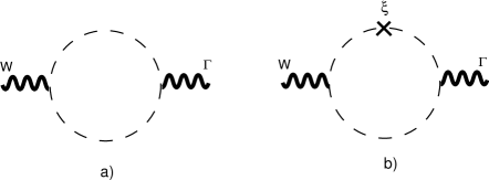
Figure 1: Diagrams contributing to $\Gamma_{\xi}^{1loop}$.

The diagram involved is shown in Figure 1-a) and yields [14]

$$\frac{3C_{A}}{2}~{}\int d^{4}xd^{4}yd^{4}\theta\,{\bf W}^{\alpha}(x)\boldsymbol{\Gamma}_{\alpha}(y)\Delta^{2}(x-y)$$

$$~{}~{}~{}~{}~{}\stackrel{{\scriptstyle R}}{{\rightarrow}}~{}-~{}\frac{3C_{A}}{4^{3}\pi^{2}}\int d^{4}xd^{4}yd^{2}\theta{\bf W}^{\alpha}(x){\bf W}_{\alpha}(y){\mathop{\mathchoice{\vbox{\vbox{\hrule height=0.4pt\hbox{\vrule width=0.4pt,height=6.0pt\kern 6.0pt\vrule width=0.4pt} \hrule height=0.4pt}}}{\vbox{\vbox{\hrule height=0.4pt\hbox{\vrule width=0.4pt,height=6.0pt\kern 6.0pt\vrule width=0.4pt} \hrule height=0.4pt}}}{\vbox{\vbox{\hrule height=0.4pt\hbox{\vrule width=0.4pt,height=3.75pt\kern 3.75pt\vrule width=0.4pt} \hrule height=0.4pt}}}{\vbox{\vbox{\hrule height=0.4pt\hbox{\vrule width=0.4pt,height=3.0pt\kern 3.0pt\vrule width=0.4pt} \hrule height=0.4pt}}}}\nolimits}\left[\Delta(x-y)\ln(x-y)^{2}M^{2}\rule{0.0pt}{11.38109pt}\right]$$ (4.3)

after use of (2.1) with $a_{UV}=0$. Here the free propagator is $\displaystyle\Delta(x)\equiv\frac{1}{{\mathop{\mathchoice{\vbox{\vbox{\hrule height=0.4pt\hbox{\vrule width=0.4pt,height=6.0pt\kern 6.0pt\vrule width=0.4pt} \hrule height=0.4pt}}}{\vbox{\vbox{\hrule height=0.4pt\hbox{\vrule width=0.4pt,height=6.0pt\kern 6.0pt\vrule width=0.4pt} \hrule height=0.4pt}}}{\vbox{\vbox{\hrule height=0.4pt\hbox{\vrule width=0.4pt,height=3.75pt\kern 3.75pt\vrule width=0.4pt} \hrule height=0.4pt}}}{\vbox{\vbox{\hrule height=0.4pt\hbox{\vrule width=0.4pt,height=3.0pt\kern 3.0pt\vrule width=0.4pt} \hrule height=0.4pt}}}}\nolimits}}(x)=-\frac{1}{4\pi^{2}}\frac{1}{x^{2}}$. The last term in (4.2) involves corrections to the gauge parameter. Standard $\boldsymbol{\nabla}$-algebra manipulations reduce it to

$$-\frac{\xi C_{A}}{4}\int d^{4}xd^{4}yd^{2}\theta\,{\bf W}^{\alpha}(x){\bf W}_{\alpha}(y){\mathop{\mathchoice{\vbox{\vbox{\hrule height=0.4pt\hbox{\vrule width=0.4pt,height=6.0pt\kern 6.0pt\vrule width=0.4pt} \hrule height=0.4pt}}}{\vbox{\vbox{\hrule height=0.4pt\hbox{\vrule width=0.4pt,height=6.0pt\kern 6.0pt\vrule width=0.4pt} \hrule height=0.4pt}}}{\vbox{\vbox{\hrule height=0.4pt\hbox{\vrule width=0.4pt,height=3.75pt\kern 3.75pt\vrule width=0.4pt} \hrule height=0.4pt}}}{\vbox{\vbox{\hrule height=0.4pt\hbox{\vrule width=0.4pt,height=3.0pt\kern 3.0pt\vrule width=0.4pt} \hrule height=0.4pt}}}}\nolimits}\left[\rule{0.0pt}{11.38109pt}\Delta(x-y)\int d^{4}z\Delta(z-y)\Delta(z-x)\right]$$ (4.4)

The integral that remains to be done corresponds to the insertion diagram of figure 1b), and diverges logarithmically for large $|z|$. This is the first instance of an off-shell IR singularity, that we renormalize along the lines explained in Section 2:

$$\int d^{4}z\;\frac{1}{(x-z)^{2}}\frac{1}{(z-y)^{2}} = \int d^{4}p\;\frac{1}{p^{4}}e^{-ip(x-y)}$$ (4.5)

$$\stackrel{{\scriptstyle\tilde{R}}}{{\rightarrow}} -\frac{1}{4}\int d^{4}p\;{\mathop{\mathchoice{\vbox{\vbox{\hrule height=0.4pt\hbox{\vrule width=0.4pt,height=6.0pt\kern 6.0pt\vrule width=0.4pt} \hrule height=0.4pt}}}{\vbox{\vbox{\hrule height=0.4pt\hbox{\vrule width=0.4pt,height=6.0pt\kern 6.0pt\vrule width=0.4pt} \hrule height=0.4pt}}}{\vbox{\vbox{\hrule height=0.4pt\hbox{\vrule width=0.4pt,height=3.75pt\kern 3.75pt\vrule width=0.4pt} \hrule height=0.4pt}}}{\vbox{\vbox{\hrule height=0.4pt\hbox{\vrule width=0.4pt,height=3.0pt\kern 3.0pt\vrule width=0.4pt} \hrule height=0.4pt}}}}\nolimits}_{p}\frac{\ln\frac{p^{2}}{\bar{M}_{IR}^{2}}}{p^{2}}e^{-ip(x-y)}$$

$$= -\pi^{2}\ln(x-y)^{2}M^{2}_{IR}\;.$$

We have used the identity (2.2) with $a_{IR}=0$. In the end we obtain the following contribution to linear order in $\xi$:

$$\frac{\xi C_{A}}{4^{3}\pi^{2}}{\mathop{\mathchoice{\vbox{\vbox{\hrule height=0.4pt\hbox{\vrule width=0.4pt,height=6.0pt\kern 6.0pt\vrule width=0.4pt} \hrule height=0.4pt}}}{\vbox{\vbox{\hrule height=0.4pt\hbox{\vrule width=0.4pt,height=6.0pt\kern 6.0pt\vrule width=0.4pt} \hrule height=0.4pt}}}{\vbox{\vbox{\hrule height=0.4pt\hbox{\vrule width=0.4pt,height=3.75pt\kern 3.75pt\vrule width=0.4pt} \hrule height=0.4pt}}}{\vbox{\vbox{\hrule height=0.4pt\hbox{\vrule width=0.4pt,height=3.0pt\kern 3.0pt\vrule width=0.4pt} \hrule height=0.4pt}}}}\nolimits}[\Delta(x-y)\ln(x-y)^{2}M_{IR}^{2}]\;,$$ (4.6)

and the full one-loop contribution results in

$$\Gamma^{1loop}_{\xi} = -\frac{C_{A}}{4^{3}\pi^{2}}\int d^{4}xd^{4}yd^{2}\theta\,{\bf W}^{\alpha}(x){\bf W}_{\alpha}(y){\mathop{\mathchoice{\vbox{\vbox{\hrule height=0.4pt\hbox{\vrule width=0.4pt,height=6.0pt\kern 6.0pt\vrule width=0.4pt} \hrule height=0.4pt}}}{\vbox{\vbox{\hrule height=0.4pt\hbox{\vrule width=0.4pt,height=6.0pt\kern 6.0pt\vrule width=0.4pt} \hrule height=0.4pt}}}{\vbox{\vbox{\hrule height=0.4pt\hbox{\vrule width=0.4pt,height=3.75pt\kern 3.75pt\vrule width=0.4pt} \hrule height=0.4pt}}}{\vbox{\vbox{\hrule height=0.4pt\hbox{\vrule width=0.4pt,height=3.0pt\kern 3.0pt\vrule width=0.4pt} \hrule height=0.4pt}}}}\nolimits}\left[\rule{0.0pt}{11.38109pt}3\Delta(x-y)\ln((x-y)^{2}M^{2})\right.$$ (4.7)

$$~{}~{}~{}~{}~{}~{}~{}~{}~{}~{}~{}~{}~{}\left.\rule{0.0pt}{11.38109pt}\mbox{}-\xi\Delta(x-y)\ln((x-y)^{2}M_{IR}^{2})\right]+{\cal O}(\xi^{2})+\ldots$$

4.2 Two Loops

We will compute the two-loop contribution in the Feynman gauge, $\xi=0$. From (3.8), the higher-loop contributions come from the expansion of a vacuum diagram with propagators and vertices made out of background covariant derivatives (Figure 2). In particular there is a single such diagram at two loops, as shown in [5].

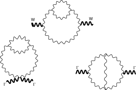
Figure 2: Diagrams contributing to $G^{(2)}$ at two loops.

After performing the $\boldsymbol{\nabla}$-algebra we find the following nonvanishing contributions (up to a common factor $-3g^{2}C^{2}_{A}/2$):

$$D_{1} = i\int d^{4}xd^{4}yd^{4}\theta\;\bar{\bf W}^{\dot{\alpha}}(x,\theta){\bf W}^{\alpha}(y,\theta)~{}\sigma^{\mu}_{\alpha\dot{\alpha}}~{}[-\Delta(x-y)\partial_{\mu}I^{0}(x,y)~{}]\;,$$

$$D_{2} = i\int d^{4}xd^{4}yd^{4}\theta\;\bar{\bf W}^{\dot{\alpha}}(x,\theta){\bf W}^{\alpha}(y,\theta)~{}\sigma^{\mu}_{\alpha\dot{\alpha}}~{}\left[2\Delta(x-y)\partial_{\mu}I^{0}(x,y)-\partial_{\mu}(\Delta(x-y)I^{0}(x,y))\right]$$

$$D_{3} = \frac{1}{2}\int d^{4}xd^{4}yd^{4}\theta~{}{\boldsymbol{\Gamma}}^{\mu}(x,\theta){\boldsymbol{\Gamma}}^{\nu}(y,\theta)\left[-\partial_{\mu}\partial_{\nu}(\Delta I^{0}(x,y))\right.$$

$$~{}~{}~{}~{}~{}~{}~{}~{}~{}~{}~{}~{}~{}~{}~{}~{}~{}~{}~{}~{}~{}~{}~{}~{}~{}~{}~{}~{}~{}~{}\left.~{}~{}~{}+4\partial_{\mu}((\partial_{\nu}\Delta)I^{0}(x,y))-4((\partial_{\mu}\partial_{\nu}\Delta)I^{0}(x,y))\right]\;,$$

$$D_{4} = {\frac{1}{2}}\int d^{4}xd^{4}yd^{4}\theta\;{\boldsymbol{\Gamma}}^{\mu}(x,\theta){\boldsymbol{\Gamma}}^{\nu}(y,\theta)~{}\left(I_{\mu\nu}^{1}(x,y)-I^{2}_{\mu\nu}(x,y)\right)\;,$$

$$D_{5} = \frac{1}{2}\int d^{4}xd^{4}yd^{4}\theta\;{\boldsymbol{\Gamma}}^{\mu}(x,\theta){\boldsymbol{\Gamma}}^{\nu}(y,\theta)~{}\delta_{\mu\nu}~{}({\mathop{\mathchoice{\vbox{\vbox{\hrule height=0.4pt\hbox{\vrule width=0.4pt,height=6.0pt\kern 6.0pt\vrule width=0.4pt} \hrule height=0.4pt}}}{\vbox{\vbox{\hrule height=0.4pt\hbox{\vrule width=0.4pt,height=6.0pt\kern 6.0pt\vrule width=0.4pt} \hrule height=0.4pt}}}{\vbox{\vbox{\hrule height=0.4pt\hbox{\vrule width=0.4pt,height=3.75pt\kern 3.75pt\vrule width=0.4pt} \hrule height=0.4pt}}}{\vbox{\vbox{\hrule height=0.4pt\hbox{\vrule width=0.4pt,height=3.0pt\kern 3.0pt\vrule width=0.4pt} \hrule height=0.4pt}}}}\nolimits}\Delta(x-y))I^{0}(x,y)\;.$$

Here and in the following, all derivatives act on $x$ unless otherwise stated. In $D_{5}$ we have replaced $\delta(x)$ by ${\mathop{\mathchoice{\vbox{\vbox{\hrule height=0.4pt\hbox{\vrule width=0.4pt,height=6.0pt\kern 6.0pt\vrule width=0.4pt} \hrule height=0.4pt}}}{\vbox{\vbox{\hrule height=0.4pt\hbox{\vrule width=0.4pt,height=6.0pt\kern 6.0pt\vrule width=0.4pt} \hrule height=0.4pt}}}{\vbox{\vbox{\hrule height=0.4pt\hbox{\vrule width=0.4pt,height=3.75pt\kern 3.75pt\vrule width=0.4pt} \hrule height=0.4pt}}}{\vbox{\vbox{\hrule height=0.4pt\hbox{\vrule width=0.4pt,height=3.0pt\kern 3.0pt\vrule width=0.4pt} \hrule height=0.4pt}}}}\nolimits}\Delta(x-y)$. The integrals $I^{i}$ are defined as follows:

$$I^{0}(x,y) = \int d^{4}ud^{4}v~{}\Delta(x-u)\Delta(y-v)\Delta^{2}(u-v)~{}~{}~{}~{}$$

$$I^{1}_{\mu\nu}(x,y) = \rule{0.0pt}{19.91692pt}\int d^{4}ud^{4}v~{}\Delta(u-v)\,\Delta(x-v)\partial_{\mu}^{x}\Delta(x-u)\,\Delta(y-v)\partial_{\nu}^{y}\Delta(y-u)$$ (4.9)

$$I^{2}_{\mu\nu}(x,y) = \int d^{4}ud^{4}v~{}\Delta(u-v)\,\Delta(x-u)\partial_{\mu}^{x}\Delta(x-v)\,\rule{0.0pt}{19.91692pt}\Delta(y-v)\partial_{\nu}^{y}\Delta(y-u).$$

As shown above, all expressions but $D_{4}$ are obtained from a single integral $I^{0}$, which is both UV and IR logarithmically divergent. On the other hand, derivatives of $I^{0}(x)$ are just UV divergent. The integrals $I^{1}$ and $I^{2}$, which appear in $D_{4}$, are IR safe as well.

The strategy now is to look for a renormalized expression for the sum $\sum_{i=1}^{5}D_{i}$. To begin with we renormalize the integral $I^{0}$. We must first cure the UV subdivergence, using the DiffR identity (2.1) with $a_{UV}=0$:

$$I^{0} = \frac{1}{(4\pi^{2})^{4}}\int d^{4}ud^{4}v\;\frac{1}{(x-u)^{2}}\frac{1}{(y-v)^{2}}\frac{1}{(u-v)^{4}}\;.$$ (4.10)

$$\stackrel{{\scriptstyle R}}{{\longrightarrow}} -\frac{1}{4(4\pi^{2})^{4}}\int d^{4}ud^{4}v\;\frac{1}{(x-u)^{2}}\frac{1}{(y-v)^{2}}{\mathop{\mathchoice{\vbox{\vbox{\hrule height=0.4pt\hbox{\vrule width=0.4pt,height=6.0pt\kern 6.0pt\vrule width=0.4pt} \hrule height=0.4pt}}}{\vbox{\vbox{\hrule height=0.4pt\hbox{\vrule width=0.4pt,height=6.0pt\kern 6.0pt\vrule width=0.4pt} \hrule height=0.4pt}}}{\vbox{\vbox{\hrule height=0.4pt\hbox{\vrule width=0.4pt,height=3.75pt\kern 3.75pt\vrule width=0.4pt} \hrule height=0.4pt}}}{\vbox{\vbox{\hrule height=0.4pt\hbox{\vrule width=0.4pt,height=3.0pt\kern 3.0pt\vrule width=0.4pt} \hrule height=0.4pt}}}}\nolimits}^{u}\frac{\ln(u-v)^{2}M^{2}}{(u-v)^{2}}$$

$$= \frac{1}{4(4\pi^{2})^{3}}\int d^{4}v\frac{1}{(y-v)^{2}}\frac{\ln(x-v)^{2}M^{2}}{(x-v)^{2}}$$

$$= -\frac{1}{4(4\pi^{2})^{3}}\int d^{4}p\;\frac{\ln p^{2}/\bar{M}^{2}}{p^{4}}e^{-ip(x-y)}\;.$$

We are left with an IR divergent expression, which is renormalized using the identity (2.4) (with $a_{IR}=0$). Integrating by parts and Fourier transforming back into $x$ space we finally find

$$I^{0}_{R}=\frac{1}{32(4\pi^{2})^{2}}\left[\ln^{2}(x-y)^{2}M^{2}_{IR}+2\ln(x-y)^{2}M^{2}_{IR}\left(1-\ln(x-y)^{2}M^{2}\right)+b_{IR}\right]$$ (4.11)

Using this result we readily obtain, with $\kappa=1/(4\pi)^{4}$,

$$D_{1}+D_{2} = -i\int d^{4}xd^{4}yd^{4}\theta\;{\bf W}^{\alpha}(x,\theta)\bar{\bf W}^{\dot{\alpha}}(y,\theta)\times$$ (4.12)

$$~{}~{}~{}~{}\sigma^{\mu}_{\alpha\dot{\alpha}}\partial_{\mu}\left(-\kappa\Delta(x\!-\!y)\ln(x\!-\!y)^{2}M^{2}+\Delta(x\!-\!y)I^{0}_{R}(x\!-\!y)\right)\;,$$

which, through the use of Bianchi identities $\boldsymbol{\nabla}^{\alpha}{\bf W}_{\alpha}=\bar{\boldsymbol{\nabla}}^{\dot{\alpha}}\bar{\bf W}_{\dot{\alpha}}$, can be written as an F term:

$$D_{1}+D_{2} = -\int d^{4}xd^{4}yd^{2}\theta\;{\bf W}^{\alpha}(x,\theta){\bf W}_{\alpha}(y,\theta)\times$$ (4.13)

$$~{}~{}~{}~{}~{}~{}{\mathop{\mathchoice{\vbox{\vbox{\hrule height=0.4pt\hbox{\vrule width=0.4pt,height=6.0pt\kern 6.0pt\vrule width=0.4pt} \hrule height=0.4pt}}}{\vbox{\vbox{\hrule height=0.4pt\hbox{\vrule width=0.4pt,height=6.0pt\kern 6.0pt\vrule width=0.4pt} \hrule height=0.4pt}}}{\vbox{\vbox{\hrule height=0.4pt\hbox{\vrule width=0.4pt,height=3.75pt\kern 3.75pt\vrule width=0.4pt} \hrule height=0.4pt}}}{\vbox{\vbox{\hrule height=0.4pt\hbox{\vrule width=0.4pt,height=3.0pt\kern 3.0pt\vrule width=0.4pt} \hrule height=0.4pt}}}}\nolimits}\left(\kappa\Delta(x-y)\ln(x\!-\!y)^{2}M^{2}-\Delta(x-y)I^{0}_{R}(x-y)\right)\;.$$

To calculate $D_{3}+D_{5}$ it is convenient to decompose the last term of $D_{3}$ (which has an overall divergence) into trace and traceless parts:

$$4\left[(\partial_{\mu}\partial_{\nu}\Delta)I^{0}\right]_{R}=\left[((4\partial_{\mu}\partial_{\nu}-\delta_{\mu\nu}{\mathop{\mathchoice{\vbox{\vbox{\hrule height=0.4pt\hbox{\vrule width=0.4pt,height=6.0pt\kern 6.0pt\vrule width=0.4pt} \hrule height=0.4pt}}}{\vbox{\vbox{\hrule height=0.4pt\hbox{\vrule width=0.4pt,height=6.0pt\kern 6.0pt\vrule width=0.4pt} \hrule height=0.4pt}}}{\vbox{\vbox{\hrule height=0.4pt\hbox{\vrule width=0.4pt,height=3.75pt\kern 3.75pt\vrule width=0.4pt} \hrule height=0.4pt}}}{\vbox{\vbox{\hrule height=0.4pt\hbox{\vrule width=0.4pt,height=3.0pt\kern 3.0pt\vrule width=0.4pt} \hrule height=0.4pt}}}}\nolimits})\Delta)I^{0}\right]_{R}+\delta_{\mu\nu}\left[({\mathop{\mathchoice{\vbox{\vbox{\hrule height=0.4pt\hbox{\vrule width=0.4pt,height=6.0pt\kern 6.0pt\vrule width=0.4pt} \hrule height=0.4pt}}}{\vbox{\vbox{\hrule height=0.4pt\hbox{\vrule width=0.4pt,height=6.0pt\kern 6.0pt\vrule width=0.4pt} \hrule height=0.4pt}}}{\vbox{\vbox{\hrule height=0.4pt\hbox{\vrule width=0.4pt,height=3.75pt\kern 3.75pt\vrule width=0.4pt} \hrule height=0.4pt}}}{\vbox{\vbox{\hrule height=0.4pt\hbox{\vrule width=0.4pt,height=3.0pt\kern 3.0pt\vrule width=0.4pt} \hrule height=0.4pt}}}}\nolimits}\Delta)I^{0}\right]_{R}+c\,\delta_{\mu\nu}\delta(x-y)\;.$$ (4.14)

According to CDR, we have included a local term that can appear in the trace-traceless decomposition at the renormalized level [23]. We shall fix its coefficient later on requiring gauge invariance. Up to this term, the trace cancels the complete diagram $D_{5}$. The rest of $D_{3}$ is overall UV finite. Renormalizing the subdivergences we find, after some algebra,

$$D_{3}+D_{5} = \int d^{4}xd^{4}yd^{4}\theta~{}\boldsymbol{\Gamma}^{\mu}(x,\theta)\boldsymbol{\Gamma}^{\nu}(y,\theta)$$ (4.15)

$$\times\mbox{}\left\{\rule{0.0pt}{19.91692pt}\right.(\partial_{\mu}\partial_{\nu}-\delta_{\mu\nu}{\mathop{\mathchoice{\vbox{\vbox{\hrule height=0.4pt\hbox{\vrule width=0.4pt,height=6.0pt\kern 6.0pt\vrule width=0.4pt} \hrule height=0.4pt}}}{\vbox{\vbox{\hrule height=0.4pt\hbox{\vrule width=0.4pt,height=6.0pt\kern 6.0pt\vrule width=0.4pt} \hrule height=0.4pt}}}{\vbox{\vbox{\hrule height=0.4pt\hbox{\vrule width=0.4pt,height=3.75pt\kern 3.75pt\vrule width=0.4pt} \hrule height=0.4pt}}}{\vbox{\vbox{\hrule height=0.4pt\hbox{\vrule width=0.4pt,height=3.0pt\kern 3.0pt\vrule width=0.4pt} \hrule height=0.4pt}}}}\nolimits})\left(-\frac{1}{2}\Delta(x-y)I^{0}_{\cal R}(x-y)+\kappa\,\Delta(x-y)\left[\ln(x-y)^{2}{M}^{2}+{\frac{1}{2}}\right]\right)$$

$$~{}~{}~{}+~{}\delta_{\mu\nu}\,\left[\frac{\kappa}{4}\,{\mathop{\mathchoice{\vbox{\vbox{\hrule height=0.4pt\hbox{\vrule width=0.4pt,height=6.0pt\kern 6.0pt\vrule width=0.4pt} \hrule height=0.4pt}}}{\vbox{\vbox{\hrule height=0.4pt\hbox{\vrule width=0.4pt,height=6.0pt\kern 6.0pt\vrule width=0.4pt} \hrule height=0.4pt}}}{\vbox{\vbox{\hrule height=0.4pt\hbox{\vrule width=0.4pt,height=3.75pt\kern 3.75pt\vrule width=0.4pt} \hrule height=0.4pt}}}{\vbox{\vbox{\hrule height=0.4pt\hbox{\vrule width=0.4pt,height=3.0pt\kern 3.0pt\vrule width=0.4pt} \hrule height=0.4pt}}}}\nolimits}\left(\Delta(x-y)\ln(x-y)^{2}{M}^{2}\right)+e\,\delta(x-y)\right]\left.\rule{0.0pt}{19.91692pt}\right\}.$$

With $e=\frac{3}{8}\kappa+\frac{c}{2}$. The non-trasverse pieces in the last line must be cancelled by $D_{4}$. Let us consider this contribution next. Again, it is convenient to split it into traceless and trace parts:

$$I^{1}_{R\,\mu\nu}-I^{2}_{R\,\mu\nu}=(I^{1}_{\mu\nu}-\frac{\delta_{\mu\nu}}{4}I^{1})-(I^{2}_{\mu\nu}-\frac{\delta_{\mu\nu}}{4}I^{2})+\frac{\delta_{\mu\nu}}{4}(I^{1}_{R\,\rho\rho}-I^{2}_{R\,\rho\rho})+c^{\prime}\delta_{\mu\nu}\delta(x-y)\,.$$ (4.16)

We have included again an arbitrary local term in the trace-traceless decomposition. The trace can be computed using Gegenbauer polynomials [13, 14]. (Alternatively, its scale dependent part can be easily obtained with “systematic” DiffR [27].) The traceless part is UV and IR finite. Therefore, it is fixed by dimensionality and by the traceless condition to be of the form $a(\partial_{\mu}\partial_{\nu}-\frac{\delta_{\mu\nu}}{4}{\mathop{\mathchoice{\vbox{\vbox{\hrule height=0.4pt\hbox{\vrule width=0.4pt,height=6.0pt\kern 6.0pt\vrule width=0.4pt} \hrule height=0.4pt}}}{\vbox{\vbox{\hrule height=0.4pt\hbox{\vrule width=0.4pt,height=6.0pt\kern 6.0pt\vrule width=0.4pt} \hrule height=0.4pt}}}{\vbox{\vbox{\hrule height=0.4pt\hbox{\vrule width=0.4pt,height=3.75pt\kern 3.75pt\vrule width=0.4pt} \hrule height=0.4pt}}}{\vbox{\vbox{\hrule height=0.4pt\hbox{\vrule width=0.4pt,height=3.0pt\kern 3.0pt\vrule width=0.4pt} \hrule height=0.4pt}}}}\nolimits})\frac{1}{(x-y)^{2}}$. The coefficient $a$ may be determined from a rather cumbersome calculation with Feynman parameters. Adding trace and traceless parts we find

$$I^{1}_{R\,\mu\nu}-I^{2}_{R\,\mu\nu} = a(\partial_{\mu}\partial_{\nu}-\delta_{\mu\nu}{\mathop{\mathchoice{\vbox{\vbox{\hrule height=0.4pt\hbox{\vrule width=0.4pt,height=6.0pt\kern 6.0pt\vrule width=0.4pt} \hrule height=0.4pt}}}{\vbox{\vbox{\hrule height=0.4pt\hbox{\vrule width=0.4pt,height=6.0pt\kern 6.0pt\vrule width=0.4pt} \hrule height=0.4pt}}}{\vbox{\vbox{\hrule height=0.4pt\hbox{\vrule width=0.4pt,height=3.75pt\kern 3.75pt\vrule width=0.4pt} \hrule height=0.4pt}}}{\vbox{\vbox{\hrule height=0.4pt\hbox{\vrule width=0.4pt,height=3.0pt\kern 3.0pt\vrule width=0.4pt} \hrule height=0.4pt}}}}\nolimits})\Delta(x-y)$$

$$-\,\delta_{\mu\nu}{\mathop{\mathchoice{\vbox{\vbox{\hrule height=0.4pt\hbox{\vrule width=0.4pt,height=6.0pt\kern 6.0pt\vrule width=0.4pt} \hrule height=0.4pt}}}{\vbox{\vbox{\hrule height=0.4pt\hbox{\vrule width=0.4pt,height=6.0pt\kern 6.0pt\vrule width=0.4pt} \hrule height=0.4pt}}}{\vbox{\vbox{\hrule height=0.4pt\hbox{\vrule width=0.4pt,height=3.75pt\kern 3.75pt\vrule width=0.4pt} \hrule height=0.4pt}}}{\vbox{\vbox{\hrule height=0.4pt\hbox{\vrule width=0.4pt,height=3.0pt\kern 3.0pt\vrule width=0.4pt} \hrule height=0.4pt}}}}\nolimits}\left[\Delta(x-y)\left(\frac{\kappa}{4}\ln\,(x-y)^{2}\!{M}^{2}-(\frac{3}{4}\zeta(3)\kappa+c^{\prime}+\frac{3}{4}a)\right)\rule{0.0pt}{14.22636pt}\right]\;.$$

Adding this to (4.15) we obtain

$$D_{3}+D_{4}+D_{5} = -\frac{1}{2}\,\int d^{4}xd^{4}yd^{4}\theta~{}\boldsymbol{\Gamma}^{\mu}(x,\theta)\boldsymbol{\Gamma}^{\nu}(y,\theta)$$ (4.18)

$$~{}~{}~{}\times~{}(\partial_{\mu}\partial_{\nu}-\delta_{\mu\nu}{\mathop{\mathchoice{\vbox{\vbox{\hrule height=0.4pt\hbox{\vrule width=0.4pt,height=6.0pt\kern 6.0pt\vrule width=0.4pt} \hrule height=0.4pt}}}{\vbox{\vbox{\hrule height=0.4pt\hbox{\vrule width=0.4pt,height=6.0pt\kern 6.0pt\vrule width=0.4pt} \hrule height=0.4pt}}}{\vbox{\vbox{\hrule height=0.4pt\hbox{\vrule width=0.4pt,height=3.75pt\kern 3.75pt\vrule width=0.4pt} \hrule height=0.4pt}}}{\vbox{\vbox{\hrule height=0.4pt\hbox{\vrule width=0.4pt,height=3.0pt\kern 3.0pt\vrule width=0.4pt} \hrule height=0.4pt}}}}\nolimits})\left[\rule{0.0pt}{14.22636pt}\Delta(x-y)\left(I^{0}_{\cal R}(x-y)-2\,\kappa\ln(x\!-\!y)^{2}{M}^{2}-a\right)\right]$$

$$+\;\frac{h}{2}\int d^{4}xd^{4}yd^{4}\theta~{}\boldsymbol{\Gamma}^{\mu}(x,\theta)\boldsymbol{\Gamma}^{\nu}(y,\theta)\delta_{\mu\nu}{\mathop{\mathchoice{\vbox{\vbox{\hrule height=0.4pt\hbox{\vrule width=0.4pt,height=6.0pt\kern 6.0pt\vrule width=0.4pt} \hrule height=0.4pt}}}{\vbox{\vbox{\hrule height=0.4pt\hbox{\vrule width=0.4pt,height=6.0pt\kern 6.0pt\vrule width=0.4pt} \hrule height=0.4pt}}}{\vbox{\vbox{\hrule height=0.4pt\hbox{\vrule width=0.4pt,height=3.75pt\kern 3.75pt\vrule width=0.4pt} \hrule height=0.4pt}}}{\vbox{\vbox{\hrule height=0.4pt\hbox{\vrule width=0.4pt,height=3.0pt\kern 3.0pt\vrule width=0.4pt} \hrule height=0.4pt}}}}\nolimits}\Delta\;,$$

with $h=\frac{3}{4}\kappa(1+\zeta(3))+\frac{3}{4}a+c+c^{\prime}$. The $M$- and $M_{IR}$-dependent parts are automatically transverse, and the non transverse contribution of the scale independent local part can be set to zero (so that the sum is gauge invariant) adjusting $c$ and $c^{\prime}$ appropiately. Thanks to its transversality, we can then rewrite this expression in a form proportional to the classical action:

$$D_{3}+D_{4}+D_{5} = -\frac{3}{4}\,\int d^{4}xd^{4}yd^{2}\theta~{}{\bf W}^{\alpha}(x,\theta){\bf W}_{\alpha}(y,\theta)$$

$$~{}~{}~{}\times~{}{\mathop{\mathchoice{\vbox{\vbox{\hrule height=0.4pt\hbox{\vrule width=0.4pt,height=6.0pt\kern 6.0pt\vrule width=0.4pt} \hrule height=0.4pt}}}{\vbox{\vbox{\hrule height=0.4pt\hbox{\vrule width=0.4pt,height=6.0pt\kern 6.0pt\vrule width=0.4pt} \hrule height=0.4pt}}}{\vbox{\vbox{\hrule height=0.4pt\hbox{\vrule width=0.4pt,height=3.75pt\kern 3.75pt\vrule width=0.4pt} \hrule height=0.4pt}}}{\vbox{\vbox{\hrule height=0.4pt\hbox{\vrule width=0.4pt,height=3.0pt\kern 3.0pt\vrule width=0.4pt} \hrule height=0.4pt}}}}\nolimits}\left[\Delta(x-y)\left(\rule{0.0pt}{11.38109pt}I^{0}_{\cal R}(x-y))-2\kappa\ln(x-y)^{2}{M}^{2}-a\right)\right].$$

Summing up all diagrams and using (4.11), we finally obtain for the full 2-loop contribution in the Feynman gauge $(\xi=0)$

$$\frac{-3g^{2}C_{A}^{2}}{2}\,\sum_{i=1}^{5}D_{i} = -\frac{3g^{2}C_{A}^{2}}{4^{6}\pi^{4}}\int d^{4}xd^{4}yd^{2}\theta~{}{\bf W}^{\alpha}(x,\theta){\bf W}_{\alpha}(y,\theta)~{}{\mathop{\mathchoice{\vbox{\vbox{\hrule height=0.4pt\hbox{\vrule width=0.4pt,height=6.0pt\kern 6.0pt\vrule width=0.4pt} \hrule height=0.4pt}}}{\vbox{\vbox{\hrule height=0.4pt\hbox{\vrule width=0.4pt,height=6.0pt\kern 6.0pt\vrule width=0.4pt} \hrule height=0.4pt}}}{\vbox{\vbox{\hrule height=0.4pt\hbox{\vrule width=0.4pt,height=3.75pt\kern 3.75pt\vrule width=0.4pt} \hrule height=0.4pt}}}{\vbox{\vbox{\hrule height=0.4pt\hbox{\vrule width=0.4pt,height=3.0pt\kern 3.0pt\vrule width=0.4pt} \hrule height=0.4pt}}}}\nolimits}\,\left[\rule{0.0pt}{11.38109pt}\Delta(x-y)\right.$$

$$\times~{}\left.\left(\ln^{2}(x\!-\!y)^{2}M_{IR}^{2}+2\ln(x\!-\!y)^{2}M_{IR}^{2}(1-\ln(x\!-\!y)^{2}M^{2})+4\ln(x\!-\!y)^{2}M^{2}\rule{0.0pt}{11.38109pt}\right)\right]$$

A possible local and scale-independent contribution has been cancelled by an adequate choice of $b_{IR}$ in (4.11). We see that only single logarithms of $M$ appear in the final result, as required by renormalization group invariance (see Section 5). This fact can also be understood in the following way: For a double $M$ logarithm we must have both UV subdivergences and overall UV divergences. By power counting, only the $\boldsymbol{\Gamma}\boldsymbol{\Gamma}$ terms may contain overall UV divergences. Furthermore, the traceless parts multiplying $\boldsymbol{\Gamma}\boldsymbol{\Gamma}$ are finite and can have only single logarithms of $M$, arising from the subdivergences. But gauge invariance, i.e. transversality, forces the trace part to have the same logarithm structure, so double logarithms of $M$ are also forbidden in the complete result. The same argument shows that were the theory scale independent (i.e., finite) to $n$ loops, the background two-point function would also be scale independent to $n+1$ loops. This line of reasoning can be pushed even further if we distinguish in our calculation the two-loop UV scale, $M^{\prime}$, from the one-loop scale, $M$. Requiring transversality on $M$ and $M^{\prime}$ independently we see that $M^{\prime}$ must cancel in the final result. (This means that the coefficient $c$ contains the expression $\ln{M^{\prime}}^{2}/M^{2}$.) So, it is only the one-loop scale that appears in the renormalized two-loop function. The significance of this observation is discussed in Section 6.

5 Renormalization group equation

After adding up the partial results (4.7) and (4.2), the final renormalized expression for the background two-point function reads

$$G^{(2)}(x) = \frac{1}{2g^{2}}\delta(x)$$ (5.1)

$$\rule{0.0pt}{22.76219pt}+\frac{3C_{A}}{4^{2}(4\pi^{2})^{2}}{\mathop{\mathchoice{\vbox{\vbox{\hrule height=0.4pt\hbox{\vrule width=0.4pt,height=6.0pt\kern 6.0pt\vrule width=0.4pt} \hrule height=0.4pt}}}{\vbox{\vbox{\hrule height=0.4pt\hbox{\vrule width=0.4pt,height=6.0pt\kern 6.0pt\vrule width=0.4pt} \hrule height=0.4pt}}}{\vbox{\vbox{\hrule height=0.4pt\hbox{\vrule width=0.4pt,height=3.75pt\kern 3.75pt\vrule width=0.4pt} \hrule height=0.4pt}}}{\vbox{\vbox{\hrule height=0.4pt\hbox{\vrule width=0.4pt,height=3.0pt\kern 3.0pt\vrule width=0.4pt} \hrule height=0.4pt}}}}\nolimits}\frac{\ln(x^{2}M^{2})}{x^{2}}-\frac{\xi C_{A}}{4^{2}(4\pi^{2})^{2}}{\mathop{\mathchoice{\vbox{\vbox{\hrule height=0.4pt\hbox{\vrule width=0.4pt,height=6.0pt\kern 6.0pt\vrule width=0.4pt} \hrule height=0.4pt}}}{\vbox{\vbox{\hrule height=0.4pt\hbox{\vrule width=0.4pt,height=6.0pt\kern 6.0pt\vrule width=0.4pt} \hrule height=0.4pt}}}{\vbox{\vbox{\hrule height=0.4pt\hbox{\vrule width=0.4pt,height=3.75pt\kern 3.75pt\vrule width=0.4pt} \hrule height=0.4pt}}}{\vbox{\vbox{\hrule height=0.4pt\hbox{\vrule width=0.4pt,height=3.0pt\kern 3.0pt\vrule width=0.4pt} \hrule height=0.4pt}}}}\nolimits}\frac{\ln(x^{2}M_{IR}^{2})}{x^{2}}+{\cal O}(\xi^{2})$$

$$\rule{0.0pt}{22.76219pt}+\frac{3g^{2}C_{A}^{2}}{4^{4}(4\pi^{2})^{3}}\left\{\rule{0.0pt}{17.07164pt}{\mathop{\mathchoice{\vbox{\vbox{\hrule height=0.4pt\hbox{\vrule width=0.4pt,height=6.0pt\kern 6.0pt\vrule width=0.4pt} \hrule height=0.4pt}}}{\vbox{\vbox{\hrule height=0.4pt\hbox{\vrule width=0.4pt,height=6.0pt\kern 6.0pt\vrule width=0.4pt} \hrule height=0.4pt}}}{\vbox{\vbox{\hrule height=0.4pt\hbox{\vrule width=0.4pt,height=3.75pt\kern 3.75pt\vrule width=0.4pt} \hrule height=0.4pt}}}{\vbox{\vbox{\hrule height=0.4pt\hbox{\vrule width=0.4pt,height=3.0pt\kern 3.0pt\vrule width=0.4pt} \hrule height=0.4pt}}}}\nolimits}\frac{\ln^{2}(x^{2}M_{IR}^{2})+2\ln(x^{2}M_{IR}^{2})(1-\ln(x^{2}M^{2}))+4\ln(x^{2}M^{2})}{x^{2}}\right.$$

$$\rule{0.0pt}{22.76219pt}+{\cal O}(\xi)\left.\rule{0.0pt}{17.07164pt}\right\}+{\cal O}(g^{4})\;.$$

Due to background gauge invariance, ${\bf W}$ undergoes no wave function renormalization. Thus the renormalization group equation for this Green function reads

$$\left.\left(M\frac{\partial}{\partial M}+\beta(g)\frac{\partial}{\partial g}+\gamma_{\xi}(g)\frac{\partial}{\partial\xi}\right)G^{(2)}(x)\right|_{\xi=0}=0\;.$$ (5.2)

Note that we can only go into the Feynman gauge after evaluating the derivative with respect to $\xi$. We have not included a term $\gamma_{IR}M_{IR}\partial/\partial M_{IR}$ because in deriving the renormalization formula (2.4) we required that the UV and IR scales were independent from each other, and hence $\gamma_{IR}=M/M_{IR}\,\partial M_{IR}/\partial M=0$. In fact, $M_{IR}$ parametrizes nonlocal contributions, which are not object of UV renormalization.

We solve the renormalization group equation perturbatively to order $g^{2}$ (two loops). The first coefficient in the expansion of $\gamma_{\xi}(g)$ can be read off from the 1-loop vacuum polarization for the gauge superfield field $V$, which is calculated in the Appendix with the result $\gamma_{\xi}(g)=-\frac{3C_{A}}{4(4\pi^{2})}g^{2}+O(g^{4})$. With this input, all the nonlocal and scale dependent pieces cancel out in (5.2). This is a check of the consistency of our renormalization procedure. In particular, note that the IR scale generated in the gauge parameter at two loops is cancelled by corrections to the gauge parameter at one loop. The remaining local parts of the renormalization group equation (5.2) uniquely fix the first two coefficients of the beta function:

$$\beta_{(}g)=-\frac{3}{4}\frac{C_{A}}{8\pi^{2}}g^{3}-\frac{3}{8}\left[\frac{C_{A}}{8\pi^{2}}\right]^{2}g^{5}+{\cal O}(g^{7})$$ (5.3)

6 Discussion

Using DiffR, we have calculated the complete renormalized correlation function of two background gauge superfields in pure N=1 SYM. This calculation illustrates the power and simplicity of this method in applications to supersymmetric gauge theories. In particular, we have seen that DiffR can be employed to subtract IR divergencies as well, and that the corresponding IR scale can be clearly distinguished from the UV one. From the dependence of the two-point function on the renormalization scale we have derived the first and second coefficients of the beta function, $b_{0}$ and $b_{1}$. Furthermore, we have presented a new argument showing that the $n+1$-loop coefficient vanishes for any supersymmetric theory which is finite to $n$ loops. This important property had been proven before using DRed [6].

It is interesting to have a closer look at the way in which the two-loop coefficient of the beta function, $b_{1}$, is generated in our calculation.

1. UV one-loop subdivergencies are subtracted. This entails a one-loop wave-function renormalization of the quantum gauge superfield. The corresponding renormalized subdiagrams depend on the one-loop renormalization scale $M$ in a local way.

2. The overall UV divergencies are subtracted and a new renormalization scale $M^{\prime}$ is introduced. However, the combination of supersymmetry, gauge invariance and power counting implies that $M^{\prime}$ cancels out in the complete renormalized two-point function. On the other hand, there remains a nonlocal dependence on $M$ (see Eqs. (4.12) and (4.18)).

3. After integration over half the supercoordinates, the dependence on $M$ becomes local.

4. Finally, this local scale dependence is compensated by $b_{1}$ in the renormalization group equation. The off-shell IR divergencies only play a passive rôle, as they exactly cancel in the renormalization group equation.

Summarizing, the scale associated to the one-loop renormalization of the quantum superfield is the one that gives rise to the two-loop coefficient of the beta function! This is somewhat surprising because naïvely one would think that the two-loop coefficient should have its origin in $M^{\prime}$, which is the scale associated to two-loop superficial divergencies. Should this be the case, the beta function would be purely one loop (remember that no overall scale can appear at any order $n>1$). However, we have seen explicitly in a two-loop calculation that the subdivergences play a nontrivial role. More generally, we expect that subdivergencies are responsible for all higher-order coefficients of the beta function. This agrees with the NSVZ form of the beta function. The fact that $M^{\prime}$ disappears in our method is directly related to the observation in [6] that in invariant four-dimensional regularization methods there are no divergencies after all subdivergencies have been subtracted. As we have seen, this does not imply $b_{1}=0$. Therefore, it seems that the naïve perturbative derivation of the beta function from renormalization constants needs some modification in this case. This modification is surely related to the presence of the anomaly discussed in [8, 9, 28, 29]. From this point of view, the fact that the standard derivation from renormalization constants works in DRed seems related to the fact that there are no rescaling anomalies in this method [22].

As a matter of fact, the mechanism we have just described agrees with previous calculations in which the corrections to the one-loop result arise from a one-loop anomaly [8, 9, 28, 29]. This anomaly manifests itself in different ways: as a nonzero expectation value for the operator $WW$ [8]; as the noninvariance of the measure under the rescaling of the gauge field [9]; or as the quantum breaking of either supersymmetry or holomorphy in the framework of local coupling [28, 29]. In our description, the anomaly is to be associated with the external loop, and is responsible for the promotion of the $M$ dependence into a non-vanishing nonlocal structure that eventually generates $b_{1}$. This is completely analogous to the explicit calculations in SQED performed in [8] (except for the fact that we subtract the subdivergencies). Note that even though $M^{\prime}$ cancels out, the presence of a $\infty-\infty$ UV behaviour is crucial for the anomaly to exist. On the other hand, as emphasized in [8], this nonlocal structure is nonanalytic at vanishing external momentum. Such on-shell IR divergence, which cancels after integration over the $\bar{\theta}$ coordinates, is a manifestation of the “IR side” of the anomaly [30] and should not be confused with the off-shell IR divergences that we have renormalized in our calculation. More generally, IR effects are known to be responsible for quantum corrections to F terms in the 1PI effective action [31]. The on-shell IR divergence arises from the region of virtual momenta of order the momentum of the external field. If this region is excluded, one finds $b_{1}=0$. Our subtraction of IR divergencies, on the other hand, is local in momentum space and does not modify the analiticity properties of the two-point function. The same applies to the IR subtractions in [6]. Summarizing, the two-loop coefficient of the beta function arises from a one-loop UV scale which survives at two loops only when IR effects are included.

For completeness, we discuss in the rest of this section the connection between the Gell-Mann-Low beta function we have computed (1PI beta function) and the flow of the coupling in the Wilsonian action (Wilsonian beta function). The Wilsonian effective action can be understood as the generating functional of Green functions with an IR cutoff, for external momenta smaller that this cutoff [33]. Therefore, at least in perturbation theory, the (“holomorphic”) Wilsonian coupling obeys a one-loop renormalization group flow. (For pure Super Yang-Mills this result also holds when nonperturbative effects are included.) The higher-order contributions to the physical beta function appear when calculating expectation values of the operators in the Wilsonian action [8]. On the other hand, in  [9] the “canonical” Wilsonian coupling was shown to obey instead an NSVZ flow. According to this work, in a Wilsonian setup this comes about because a rescaling of the gauge superfields at each scale is needed in order to keep kinetic terms canonically normalized. This rescaling induces an anomalous Jacobian, and it is this anomaly that induces the corrections to the one-loop result [9]. In this reference, the anomaly is calculated à la Fujikawa. A basic element of the calculation is the introduction of a UV cutoff and one might believe that the anomaly (and thus the running of the canonical coupling) depends only on the UV properties of the theory. However, a closer look shows that the low-energy degrees of freedom play a fundamental rôle [10, 30]. In fact, the IR degrees of freedom must be included in the derivation of the anomaly if low-energy physics is to remain unchanged under the field rescalings. In this sense, taking the rescaling anomaly into account is equivalent to calculating the expectation value of the Wilsonian action [8].

It was also argued in [9] (see [34] as well) that the canonical Wilsonian coupling is closely related to the 1PI running coupling. (This implies that the expectation value of the canonical Wilsonian action is basically trivial.) This relation has been made more precise, in a general context, in [35]. There it is shown that, when all kinetic terms are canonically normalized, the Wilsonian coupling becomes independent of the renormalization scale for large cutoff. Then one can derive the equation (see also [36])

$$\beta(g)=\left[\frac{\Lambda\partial/\partial\Lambda\,g_{cW}(g,\Lambda/M)}{\partial/\partial g\,g_{cW}(g,\Lambda/M)}\right]_{\Lambda\rightarrow\infty}\;.$$ (6.1)

Here $g$ is the physical coupling, $g_{cW}$ is the canonical Wilsonian coupling, $\Lambda$ is the flowing cutoff in the Wilsonian action and $M$ is the renormalization scale, introduced by low-energy normalization conditions. Using this equation, we show now that (at least for large $\Lambda$) the 1PI and the canonical Wilsonian beta functions agree to two loops in perturbation theory, as functions of $g$ and $g_{cW}$, respectively. The flow of $g_{cW}$ is of the generic form

$$\beta_{cW}(g_{cW})\equiv\Lambda\partial g_{cW}/\partial\Lambda=b_{0}g_{cW}^{3}+b_{1}g_{cW}^{5}+b_{2}g_{cW}^{7}+{\cal O}(g_{cW}^{9})\;,$$ (6.2)

with constant coefficients $b_{n}$. On the other hand, $g_{cW}$ can be perturbatively expanded in powers of $g$:

$$g_{cW}=g\left(1+C_{0}(\Lambda/M)g^{2}+C_{1}(\Lambda/M)g^{4}+{\cal O}(g^{6})\right)\;,$$ (6.3)

where we have taken $g_{cW}=g$ at tree level. Inserting (6.3) into (6.2) we see that

$$C_{0}(\Lambda/M) = b_{0}\ln\frac{\Lambda}{M}+c_{0}\;,$$

$$C_{1}(\Lambda/M) = \frac{3}{2}b_{0}^{2}\ln^{2}\frac{\Lambda}{M}+(2b_{0}c_{0}+b_{1})\ln\frac{\Lambda}{M}+c_{1}\,,$$ (6.4)

where $c_{n}$ are scheme dependent constants. Using (6.2) and (6.3) in Eq. (6.1) we find

$$\beta(g)=\left[b_{0}g^{3}+b_{1}g^{5}+(b_{2}+2b_{1}C_{0}+3b_{0}C_{0}^{2}-2b_{0}C_{1})g^{7}+{\cal O}(g^{9})\right]_{\Lambda\rightarrow\infty}\;,$$ (6.5)

and using also (6.4) we see that the beta function is finite:

$$\beta(g)=b_{0}g^{3}+b_{1}g^{5}+(b_{0}(3c_{0}^{2}-c_{1})+b_{1}c_{0}+b_{2})g^{7}+{\cal O}(g^{9})\;.$$ (6.6)

Hence, the first two coefficients of the 1PI beta function coincide, in any (mass-independent) scheme, with the first two coefficients of the canonical Wilsonian beta function. The other coefficients are scheme dependent, as expected. This scheme dependence has been studied for general N=1 theories in [37].

Appendix A Calculation of $\gamma_{\xi}$

The classical action in a generic Lorentz gauge reads

$$S = -\frac{1}{2g^{2}}\int d^{8}z\;(e^{-gV}D^{\alpha}e^{gV})\bar{D}^{2}(e^{-gV}D_{\alpha}e^{gV})-(\xi+1)\int d^{8}z\;(D^{2}V)(\bar{D}^{2}V)\;.$$ (A.1)

To second order in the quantum field $V$ it reduces to

$$S^{(2)} = \frac{1}{2}\int d^{8}z\;VD^{\alpha}\bar{D}^{2}D_{\alpha}V-\frac{(\xi+1)}{2}\int d^{8}z\;V(D^{2}\bar{D}^{2}+\bar{D}^{2}D^{2})V$$ (A.2)

$$= -\frac{1}{2}\int d^{8}z\;V{\mathop{\mathchoice{\vbox{\vbox{\hrule height=0.4pt\hbox{\vrule width=0.4pt,height=6.0pt\kern 6.0pt\vrule width=0.4pt} \hrule height=0.4pt}}}{\vbox{\vbox{\hrule height=0.4pt\hbox{\vrule width=0.4pt,height=6.0pt\kern 6.0pt\vrule width=0.4pt} \hrule height=0.4pt}}}{\vbox{\vbox{\hrule height=0.4pt\hbox{\vrule width=0.4pt,height=3.75pt\kern 3.75pt\vrule width=0.4pt} \hrule height=0.4pt}}}{\vbox{\vbox{\hrule height=0.4pt\hbox{\vrule width=0.4pt,height=3.0pt\kern 3.0pt\vrule width=0.4pt} \hrule height=0.4pt}}}}\nolimits}\Pi_{1/2}V-\frac{(\xi+1)}{2}d^{8}zV{\mathop{\mathchoice{\vbox{\vbox{\hrule height=0.4pt\hbox{\vrule width=0.4pt,height=6.0pt\kern 6.0pt\vrule width=0.4pt} \hrule height=0.4pt}}}{\vbox{\vbox{\hrule height=0.4pt\hbox{\vrule width=0.4pt,height=6.0pt\kern 6.0pt\vrule width=0.4pt} \hrule height=0.4pt}}}{\vbox{\vbox{\hrule height=0.4pt\hbox{\vrule width=0.4pt,height=3.75pt\kern 3.75pt\vrule width=0.4pt} \hrule height=0.4pt}}}{\vbox{\vbox{\hrule height=0.4pt\hbox{\vrule width=0.4pt,height=3.0pt\kern 3.0pt\vrule width=0.4pt} \hrule height=0.4pt}}}}\nolimits}\Pi_{0}V\;,$$

were we have defined the projectors

$$\Pi_{1/2} = -\frac{D^{\alpha}\bar{D}^{2}D_{\alpha}}{{\mathop{\mathchoice{\vbox{\vbox{\hrule height=0.4pt\hbox{\vrule width=0.4pt,height=6.0pt\kern 6.0pt\vrule width=0.4pt} \hrule height=0.4pt}}}{\vbox{\vbox{\hrule height=0.4pt\hbox{\vrule width=0.4pt,height=6.0pt\kern 6.0pt\vrule width=0.4pt} \hrule height=0.4pt}}}{\vbox{\vbox{\hrule height=0.4pt\hbox{\vrule width=0.4pt,height=3.75pt\kern 3.75pt\vrule width=0.4pt} \hrule height=0.4pt}}}{\vbox{\vbox{\hrule height=0.4pt\hbox{\vrule width=0.4pt,height=3.0pt\kern 3.0pt\vrule width=0.4pt} \hrule height=0.4pt}}}}\nolimits}}$$ (A.3)

$$\Pi_{0} = \frac{D^{2}\bar{D}^{2}+\bar{D}^{2}D^{2}}{{\mathop{\mathchoice{\vbox{\vbox{\hrule height=0.4pt\hbox{\vrule width=0.4pt,height=6.0pt\kern 6.0pt\vrule width=0.4pt} \hrule height=0.4pt}}}{\vbox{\vbox{\hrule height=0.4pt\hbox{\vrule width=0.4pt,height=6.0pt\kern 6.0pt\vrule width=0.4pt} \hrule height=0.4pt}}}{\vbox{\vbox{\hrule height=0.4pt\hbox{\vrule width=0.4pt,height=3.75pt\kern 3.75pt\vrule width=0.4pt} \hrule height=0.4pt}}}{\vbox{\vbox{\hrule height=0.4pt\hbox{\vrule width=0.4pt,height=3.0pt\kern 3.0pt\vrule width=0.4pt} \hrule height=0.4pt}}}}\nolimits}}\;.$$ (A.4)

The one-loop correction to this quadratic action can be easily computed. The result in the Feynman gauge is

$$\Gamma = -\frac{3C_{A}g^{2}}{4(4\pi^{2})^{2}}\int d^{8}z_{1}d^{8}z_{2}\;V(z_{1})D^{\alpha}\bar{D}^{2}D_{\alpha}V(z_{2})\delta_{12}\frac{1}{(x_{1}-x_{2})^{4}}$$ (A.5)

$$\stackrel{{\scriptstyle R}}{{\rightarrow}} -\frac{3C_{A}g^{2}}{16(4\pi^{2})}\int d^{8}z_{1}d^{8}z_{2}\;V(z_{1})D^{\alpha}\bar{D}^{2}D_{\alpha}V(z_{2})\delta_{12}{\mathop{\mathchoice{\vbox{\vbox{\hrule height=0.4pt\hbox{\vrule width=0.4pt,height=6.0pt\kern 6.0pt\vrule width=0.4pt} \hrule height=0.4pt}}}{\vbox{\vbox{\hrule height=0.4pt\hbox{\vrule width=0.4pt,height=6.0pt\kern 6.0pt\vrule width=0.4pt} \hrule height=0.4pt}}}{\vbox{\vbox{\hrule height=0.4pt\hbox{\vrule width=0.4pt,height=3.75pt\kern 3.75pt\vrule width=0.4pt} \hrule height=0.4pt}}}{\vbox{\vbox{\hrule height=0.4pt\hbox{\vrule width=0.4pt,height=3.0pt\kern 3.0pt\vrule width=0.4pt} \hrule height=0.4pt}}}}\nolimits}\left[\Delta(x_{12})\ln x_{12}^{2}M^{2}\right]\;.$$

Therefore, the one loop effective action quadratic in the quantum gauge field is

$$\Gamma = \int d^{8}z_{1}d^{8}z_{2}\;V(z_{1})\Gamma^{(2)}(z_{1},z_{2})V(z_{2})$$ (A.6)

$$= \int d^{8}z_{1}d^{8}z_{2}\;V(z_{1})\left[-\frac{1}{2}\delta^{(8)}(z_{12}){\mathop{\mathchoice{\vbox{\vbox{\hrule height=0.4pt\hbox{\vrule width=0.4pt,height=6.0pt\kern 6.0pt\vrule width=0.4pt} \hrule height=0.4pt}}}{\vbox{\vbox{\hrule height=0.4pt\hbox{\vrule width=0.4pt,height=6.0pt\kern 6.0pt\vrule width=0.4pt} \hrule height=0.4pt}}}{\vbox{\vbox{\hrule height=0.4pt\hbox{\vrule width=0.4pt,height=3.75pt\kern 3.75pt\vrule width=0.4pt} \hrule height=0.4pt}}}{\vbox{\vbox{\hrule height=0.4pt\hbox{\vrule width=0.4pt,height=3.0pt\kern 3.0pt\vrule width=0.4pt} \hrule height=0.4pt}}}}\nolimits}\Pi_{1/2}-\frac{(\xi+1)}{2}\delta^{(8)}(z_{12}){\mathop{\mathchoice{\vbox{\vbox{\hrule height=0.4pt\hbox{\vrule width=0.4pt,height=6.0pt\kern 6.0pt\vrule width=0.4pt} \hrule height=0.4pt}}}{\vbox{\vbox{\hrule height=0.4pt\hbox{\vrule width=0.4pt,height=6.0pt\kern 6.0pt\vrule width=0.4pt} \hrule height=0.4pt}}}{\vbox{\vbox{\hrule height=0.4pt\hbox{\vrule width=0.4pt,height=3.75pt\kern 3.75pt\vrule width=0.4pt} \hrule height=0.4pt}}}{\vbox{\vbox{\hrule height=0.4pt\hbox{\vrule width=0.4pt,height=3.0pt\kern 3.0pt\vrule width=0.4pt} \hrule height=0.4pt}}}}\nolimits}\Pi_{0}-\right.$$

$$+ \left.\frac{3C_{A}g^{2}}{16(4\pi^{2})}\left({\mathop{\mathchoice{\vbox{\vbox{\hrule height=0.4pt\hbox{\vrule width=0.4pt,height=6.0pt\kern 6.0pt\vrule width=0.4pt} \hrule height=0.4pt}}}{\vbox{\vbox{\hrule height=0.4pt\hbox{\vrule width=0.4pt,height=6.0pt\kern 6.0pt\vrule width=0.4pt} \hrule height=0.4pt}}}{\vbox{\vbox{\hrule height=0.4pt\hbox{\vrule width=0.4pt,height=3.75pt\kern 3.75pt\vrule width=0.4pt} \hrule height=0.4pt}}}{\vbox{\vbox{\hrule height=0.4pt\hbox{\vrule width=0.4pt,height=3.0pt\kern 3.0pt\vrule width=0.4pt} \hrule height=0.4pt}}}}\nolimits}\left[\Delta(x_{12}^{2})\ln x_{12}^{2}M^{2}\right]{\mathop{\mathchoice{\vbox{\vbox{\hrule height=0.4pt\hbox{\vrule width=0.4pt,height=6.0pt\kern 6.0pt\vrule width=0.4pt} \hrule height=0.4pt}}}{\vbox{\vbox{\hrule height=0.4pt\hbox{\vrule width=0.4pt,height=6.0pt\kern 6.0pt\vrule width=0.4pt} \hrule height=0.4pt}}}{\vbox{\vbox{\hrule height=0.4pt\hbox{\vrule width=0.4pt,height=3.75pt\kern 3.75pt\vrule width=0.4pt} \hrule height=0.4pt}}}{\vbox{\vbox{\hrule height=0.4pt\hbox{\vrule width=0.4pt,height=3.0pt\kern 3.0pt\vrule width=0.4pt} \hrule height=0.4pt}}}}\nolimits}\Pi_{1/2}+{\cal O}(\xi)\right)\right]V(z_{2})\;.$$

The renormalization group equation for the correlation function of two quantum gauge fields has the form:

$$\left.\left(M\frac{\partial}{\partial M}+\beta\frac{\partial}{\partial g}+\gamma_{\xi}\frac{\partial}{\partial\xi}-2\gamma_{V}\right)\Gamma^{(2)}\right|_{\xi=0}=0\;.$$ (A.7)

To order $g^{2}$ (one loop) it is solved for

$$\gamma_{V} = -\frac{3C_{A}}{8(4\pi^{2})}g^{2}+\ldots$$ (A.8)

$$\gamma_{\xi} = -\frac{3C_{A}}{4(4\pi^{2})}g^{2}+\ldots$$ (A.9)

References

- [1] C. P. Herzog, I. R. Klebanov and P. Ouyang [C01-07-20.4 Collaboration], arXiv:hep-th/0108101.
- [2] V. A. Novikov, M. A. Shifman, A. I. Vainshtein and V. I. Zakharov, Nucl. Phys. B 229, 381 (1983).
- [3] D. R. T. Jones, Phys. Lett. B 123, 45 (1983).
- [4] L. F. Abbott, M. T. Grisaru and D. Zanon, Nucl. Phys. B 244, 454 (1984).
- [5] M. T. Grisaru and D. Zanon, Nucl. Phys. B 252, 578 (1985).
- [6] M. T. Grisaru, B. Milewski and D. Zanon, Phys. Lett. B 155, 357 (1985).
- [7] V. A. Novikov, M. A. Shifman, A. I. Vainshtein and V. I. Zakharov, Phys. Lett. B 166, 329 (1986) [Sov. J. Nucl. Phys. 43, 294.1986 YAFIA,43,459 (1986)].
- [8] M. A. Shifman and A. I. Vainshtein, Nucl. Phys. B 277, 456 (1986) [Sov. Phys. JETP 64, 428 (1986)].
- [9] N. Arkani-Hamed and H. Murayama, JHEP 0006, 030 (2000) [arXiv:hep-th/9707133].
- [10] M. A. Shifman, Int. J. Mod. Phys. A 14, 5017 (1999) [arXiv:hep-th/9906049].
- [11] K. G. Chetyrkin and F. V. Tkachov, Phys. Lett. B 114, 340 (1982).
- [12] D. Z. Freedman, K. Johnson and J. I. Latorre, Nucl. Phys. B 371, 353 (1992).
- [13] P. E. Haagensen, Mod. Phys. Lett. A 7, 893 (1992) [arXiv:hep-th/9111015].
- [14] Yun. S. Song, MIT Archive: B.S. Thesis in Physics (1996)
- [15] F. del Aguila, A. Culatti, R. Muñoz-Tapia and M. Pérez-Victoria, Nucl. Phys. B 504, 532 (1997) [arXiv:hep-ph/9702342].
- [16] T. Hahn and M. Pérez-Victoria, Comput. Phys. Commun. 118, 153 (1999) [arXiv:hep-ph/9807565].
- [17] T. Hahn and C. Schappacher, Comput. Phys. Commun. 143, 54 (2002) [arXiv:hep-ph/0105349].
- [18] E. N. Popov, JINR-E2-84-569.
- [19] L. V. Avdeev, D. I. Kazakov and I. N. Kondrashuk, Int. J. Mod. Phys. A 9, 1067 (1994) [arXiv:hep-th/9302085].
- [20] V. A. Smirnov, Nucl. Phys. B 427, 325 (1994).
- [21] V. A. Smirnov, Theor. Math. Phys. 108, 953 (1997) [Teor. Mat. Fiz. 108N1, 129 (1997)] [arXiv:hep-th/9605162].
- [22] S. J. Gates, M. T. Grisaru, M. Rocek and W. Siegel, Front. Phys. 58, 1 (1983) [arXiv:hep-th/0108200].
- [23] F. del Aguila, A. Culatti, R. Muñoz Tapia and M. Pérez-Victoria, Nucl. Phys. B 537, 561 (1999) [arXiv:hep-ph/9806451].
- [24] F. del Aguila, A. Culatti, R. Muñoz-Tapia and M. Pérez-Victoria, Phys. Lett. B 419, 263 (1998) [arXiv:hep-th/9709067].
- [25] M. Pérez-Victoria, Phys. Lett. B 442, 315 (1998) [arXiv:hep-th/9808071].
- [26] F. del Aguila, A. Culatti, R. M. Tapia and M. Pérez-Victoria, arXiv:hep-ph/9711474.
- [27] J. I. Latorre, C. Manuel and X. Vilasis-Cardona, Annals Phys. 231, 149 (1994) [arXiv:hep-th/9303044].
- [28] E. Kraus, Nucl. Phys. B 620, 55 (2002) [arXiv:hep-th/0107239].
- [29] E. Kraus, arXiv:hep-ph/0110323.
- [30] M. A. Shifman, Phys. Rep. 209, 341 (1991).
- [31] P. West, Phys. Lett. B 261, 396 (1991).
- [32] K. i. Konishi and K. i. Shizuya, Nuovo Cim. A 90, 111 (1985).
- [33] G. Keller, C. Kopper and M. Salmhofer, Helv. Phys. Acta 65, 32 (1992).
- [34] N. Arkani-Hamed and H. Murayama, Phys. Rev. D 57, 6638 (1998) [arXiv:hep-th/9705189].
- [35] M. Bonini, G. Marchesini and M. Simionato, Nucl. Phys. B 483, 475 (1997) [arXiv:hep-th/9604114].
- [36] J.C. Collins, “Renormalization”, Cambridge University Press, Cambridge 1984.
- [37] I. Jack, D. R. Jones and C. G. North, Nucl. Phys. B 486, 479 (1997) [arXiv:hep-ph/9609325].