Dilatonic monopoles from ($4+1$)- dimensional vortices

Abstract

We study spherically and axially symmetric monopoles of the SU(2) Einstein-Yang-Mills-Higgs-dilaton (EYMHD) system with a new coupling between the dilaton field and the covariant derivative of the Higgs field. This coupling arises in the study of ($4+1$)- dimensional vortices in the Einstein-Yang-Mills (EYM) system.

1 Introduction

In the 1920s, Kaluza and Klein studied the $5$-dimensional version of the Einstein equations [1] by introducing a $5$-dimensional metric tensor. When one dimension is compactified, the equations of $4$-dimensional Einstein gravity plus Maxwell’s equations are recovered. One of the new fields appearing in this model is the dilaton, a scalar companion of the metric tensor. In an analog way, this field arises in the low energy effective action of superstring theories and is associated with the classical scale invariance of these models [2].

In recent years, a number of classical field theory models coupled to a dilaton have been studied. It was found that if the solutions of SU(2) Yang-Mills-Higgs (YMH) theory, namely the ’t Hooft-Polyakov monopole [3] and its higher winding number generalisations [4, 5, 6], are coupled to a massless dilaton [7, 8], remarkable similarities to the qualitative features of Einstein-Yang-Mills-Higgs (EYMH) monopoles [9, 10] arise. Especially, it was observed that similarly to gravity the dilaton can render attraction between like charged monopoles and thus bound multimonopole states are possible.

Recently, the YMH system coupled to both gravity and the dilaton has been studied [11, 8]. It was found that in the full Einstein-Yang-Mills-Higgs-dilaton (EYMHD) model, a simple relation between the $tt$-component of the metric and the dilaton exists. The abelian solutions to which the configurations tend in the limit of critical coupling are the extremal Einstein-Maxwell-dilaton (EMD) solutions. These have definite expressions for the energy and the value of the $rr$-component of the metric at the origin which only depend on the fundamental couplings.

Volkov argued recently [12] that if $\frac{\partial}{\partial x_{4}}$ is a symmetry of the Einstein-Yang-Mills (EYM) system in ($4+1$) dimensions, where $x_{4}$ is the coordinate associated with the $5$th dimensions, then the ($4+1$)-dimensional EYM system reduces effectively to a ($3+1$)-dimensional EYMHD system with a specific coupling between the dilaton field and the Higgs field.

In this paper, we study both the spherically and axially symmetric solutions of the ($3+1$)-dimensional EYMHD model deduced from the ($4+1$)-dimensional EYM system. In Section 2, we give the EYMHD Lagrangian and review how the specific coupling arises. In Sections 3 und 4, we give the Ansatz and present our numerical results for the spherically and axially symmetric solutions, respectively. In both these Sections emphasis is placed on the flat space limit and on the limit in which our system of equations reduces to the one in [12]. The summary and conclusions are presented in Section 5.

2 SU(2) Einstein-Yang-Mills-Higgs-dilaton theory

The Lagrangian and the particular coupling of the dilaton field $\Psi$ to the SU(2) gauge fields ${A_{\mu}}^{a}$ and Higgs fields ${\Phi}^{a}$ ($a=1,2,3$), respectively, arise effectively from the Lagrangian of ($4+1$)-dimensional EYM theory. If both the matter functions and the metric functions are independent on $x_{4}$, the $5$-dimensional fields can be parametrized as follows (with $M,N=0,1,2,3,4$) [12]:

$$g^{(5)}_{MN}dx^{M}dx^{N}=e^{-\zeta}g^{(4)}_{\mu\nu}dx^{\mu}dx^{\nu}-e^{2\zeta}(dx^{4})^{2}\ ,\ \mu,\nu=0,1,2,3$$ (1)

and

$$A_{M}^{a}dx^{M}=A_{\mu}^{a}dx^{\mu}+\Phi^{a}dx^{4}\ ,\ \ a=1,2,3$$ (2)

where $g^{(4)}$ is the $4$-dimensional metric tensor and $\zeta$ plays the role of the dilaton. Introducing a new coupling $\kappa$ to study the influence of the dilaton systematically, we set $\zeta=2\kappa\Psi$ and obtain the following action of the effective $4$-dimensional EYMHD theory:

$$S=S_{G}+S_{M}=\int L_{G}\sqrt{-g^{(4)}}d^{4}x+\int L_{M}\sqrt{-g^{(4)}}d^{4}x\ .$$ (3)

The gravity Lagrangian $L_{G}$ is given by

$$L_{G}=\frac{1}{16\pi G}R\ ,$$ (4)

where $G$ is Newton‘s constant, while the matter Lagrangian $L_{M}$ reads:

$$L_{M}=-\frac{1}{4}e^{2\kappa\Psi}F_{\mu\nu}^{a}F^{\mu\nu,a}-\frac{1}{2}\partial_{\mu}\Psi\partial^{\mu}\Psi-\frac{1}{2}e^{-4\kappa\Psi}D_{\mu}\Phi^{a}D^{\mu}\Phi^{a}-e^{-2\kappa\Psi}V(\Phi^{a})\ ,$$ (5)

with Higgs potential

$$V(\Phi^{a})=\frac{\lambda}{4}(\Phi^{a}\Phi^{a}-v^{2})^{2}\ ,$$ (6)

the non-abelian field strength tensor

$$F_{\mu\nu}^{a}=\partial_{\mu}A_{\nu}^{a}-\partial_{\nu}A_{\mu}^{a}+e\varepsilon_{abc}A_{\mu}^{b}A_{\nu}^{c}\ ,$$ (7)

and the covariant derivative of the Higgs field in the adjoint representation

$$D_{\mu}\Phi^{a}=\partial_{\mu}\Phi^{a}+e\varepsilon_{abc}A_{\mu}^{b}\Phi^{c}\ .$$ (8)

Here, $e$ denotes the gauge field coupling constant, $\lambda$ the Higgs field coupling constant and $v$ the vacuum expectation value of the Higgs field.

3 Spherically symmetric solutions

For the metric, the spherically symmetric Ansatz in Schwarzschild-like coordinates reads [9]:

$$ds^{2}=g^{(4)}_{\mu\nu}dx^{\mu}dx^{\nu}=-A^{2}(r)N(r)dt^{2}+N^{-1}(r)dr^{2}+r^{2}d\theta^{2}+r^{2}\sin^{2}\theta d^{2}\varphi\ ,$$ (9)

with

$$N(r)=1-\frac{2m(r)}{r}\ .$$ (10)

In these coordinates, $m(\infty)$ denotes the (dimensionful) mass of the field configuration.

For the gauge and Higgs fields, we use the purely magnetic hedgehog ansatz [3]

$${A_{r}}^{a}={A_{t}}^{a}=0\ ,$$ (11)

$${A_{\theta}}^{a}=\frac{1-K(r)}{e}{e_{\varphi}}^{a}\ ,\ \ \ \ {A_{\varphi}}^{a}=-\frac{1-K(r)}{e}\sin\theta{e_{\theta}}^{a}\ ,$$ (12)

$${\Phi}^{a}=vH(r){e_{r}}^{a}\ .$$ (13)

The dilaton is a scalar field depending only on $r$

$$\Psi=\Psi(r)\ .$$ (14)

Inserting the Ansatz into the Lagrangian and varying with respect to the matter fields yields the Euler-Lagrange equations, while variation with respect to the metric yields the Einstein equations.

With the introduction of dimensionless coordinates and fields

$$x=evr\ ,\ \ \mu=evm\ ,\ \ \phi=\frac{\Phi}{v}\ ,\ \ \psi=\frac{\Psi}{v}\ .$$ (15)

the Lagrangian and the resulting set of differential equations depend only on three dimensionless coupling constants, $\alpha$, $\beta$ and $\gamma$,

$$\alpha=\sqrt{G}v=\frac{M_{W}}{eM_{\rm Pl}}\ ,\ \ \beta=\frac{\sqrt{\lambda}}{e}=\frac{M_{H}}{\sqrt{2}M_{W}}\ ,\ \ \gamma=\kappa v=\frac{\kappa M_{W}}{e}\ ,$$ (16)

where $M_{W}=ev$, $M_{H}=\sqrt{2\lambda}v$ and $M_{\rm Pl}=1/\sqrt{G}$. With the rescalings (15) and (16), the dimensionless mass of the solution is given by $\frac{\mu(\infty)}{\alpha^{2}}$.

With (15) and (16) the Euler-Lagrange equations read:

$$(e^{2\gamma\psi}ANK^{\prime})^{\prime}=A(e^{2\gamma\psi}\frac{K(K^{2}-1)}{x^{2}}+e^{-4\gamma\psi}H^{2}K)\ ,$$ (17)

$$(e^{-4\gamma\psi}x^{2}ANH^{\prime})^{\prime}=AH(2e^{-4\gamma\psi}K^{2}+\beta^{2}x^{2}e^{-2\gamma\psi}(H^{2}-1))\ ,$$ (18)

$$(x^{2}AN\psi^{\prime})^{\prime} = 2\gamma A[e^{2\gamma\psi}(N(K^{\prime})^{2}+\frac{(K^{2}-1)^{2}}{2x^{2}})$$ (19)

$$- e^{-2\gamma\psi}\frac{\beta^{2}x^{2}}{4}(H^{2}-1)^{2}-2e^{-4\gamma\psi}(\frac{1}{2}N(H^{\prime})^{2}x^{2}+H^{2}K^{2})]\ ,$$

where the prime denotes the derivative with respect to $x$, while we use the following combination of the Einstein equations

$$G_{tt}=2\alpha^{2}T_{tt}=-2\alpha^{2}A^{2}NL_{M}\ ,$$ (20)

$$g^{xx}G_{xx}-g^{tt}G_{tt}=-4\alpha^{2}N\frac{\partial L_{M}}{\partial N}$$ (21)

to obtain two differential equations for the two metric functions:

$$\mu^{\prime}=\alpha^{2}\left(e^{2\gamma\psi}N(K^{\prime})^{2}+\frac{1}{2}Nx^{2}(H^{\prime})^{2}e^{-4\gamma\psi}+\frac{1}{2x^{2}}(K^{2}-1)^{2}e^{2\gamma\psi}+K^{2}H^{2}e^{-4\gamma\psi}\right.$$

$$+\left.\frac{\beta^{2}}{4}x^{2}(H^{2}-1)^{2}e^{-2\gamma\psi}+\frac{1}{2}Nx^{2}(\psi^{\prime})^{2}\right)\ ,$$ (22)

$$A^{\prime}=\alpha^{2}xA\left(\frac{2(K^{\prime})^{2}}{x^{2}}e^{2\gamma\psi}+e^{-4\gamma\psi}(H^{\prime})^{2}+(\psi^{\prime})^{2}\right)\ .$$ (23)

Since we are looking for globally regular, finite energy solutions which are asymptotically flat, we impose the following set of boundary conditions:

$$K(0)=1\ ,\ \ H(0)=0\ ,\ \ \partial_{x}\psi|_{x=0}=0\ ,\ \ \mu(0)=0\ .$$ (24)

$$K(\infty)=0\ ,\ \ H(\infty)=1\ ,\ \ \psi(\infty)=0\ ,\ \ A(\infty)=1\ ,$$ (25)

3.1 Numerical results

We have restricted our numerical calculations for the spherically as well as for the axially symmetric solutions to $\beta=0$.

3.1.1 The $\alpha=0$ limit

For $\alpha=0$, the gravitational field equations (22) and (23) decouple from the rest of the system and we are left with the YMHD model in flat space, $N(x)\equiv 1$ and $A(x)\equiv 1$. In [7] it was observed that (in analogy to the EYMH system) the monopoles exist up to a maximal value of the dilaton coupling $\gamma=\gamma_{max}$ and from there on a second branch of solutions tend to the abelian solution for $\gamma\rightarrow\gamma_{cr}<\gamma_{max}$ with $\psi(0)$ monotonically decreasing to $-\infty$. Our numerical results indicate that no such $\gamma_{max}$ exists in the model studied here. We have integrated the equations for $\gamma~{}\epsilon~{}[0:10]$ and found the solutions to exist for all these values of $\gamma$. The profiles of the functions suggest that for $\gamma\rightarrow\infty$ the solutions tend to the vacuum solution with $K(x)\equiv 1$, $H(x)\equiv 0$ and $\psi(x)\equiv 0$. This is indicated by the fact that the mass of the field configurations progressively tends to zero for rising $\gamma$ and that the matter fields are equal to their vacuum values on increasing intervals of the coordinate $x$. To demonstrate this, we give below the values of $x_{K}$ and $x_{H}$, where the gauge field $K(x)$ and the Higgs field $H(x)$, respectively, reach the value $0.5$, i.e. $K(x_{K})=0.5$ and $H(x_{H})=0.5$ :

$\gamma$	$x_{K}$	$x_{H}$
$0.1$	$2.2$	$1.8$
$1.0$	$3.3$	$2.1$
$5.0$	$11.2$	$5.1$
$10.0$	$22.4$	$8.9$

Moreover, we find that $\psi(0)\geq 0$ for all $\gamma$. Since for $\gamma=0$, the BPS monopole solution is recovered, the curve for $\psi(0)$ starts from zero at $\gamma=0$. From there it increases to a maximal value at $\gamma\approx 1.38$ and then slowly decreases to zero for $\gamma\rightarrow\infty$. Together with (25) our results strongly suggest that $\psi(x)$ tends to zero on the full interval $x~{}\epsilon~{}[0:\infty[$.

The difference between the model studied here and the one studied in [7] is that in the standard case of the Yang-Mills-Higgs-dilaton system, the equations are effectively the equations of an Einstein-Yang-Mills-Higgs model with metric

$$ds^{2}=-e^{2\kappa\Psi(r)}dt^{2}+e^{-2\kappa\Psi(r)}dr^{2}+e^{-2\kappa\Psi(r)}r^{2}d\theta^{2}+e^{-2\kappa\Psi(r)}r^{2}\sin^{2}\theta d^{2}\varphi$$ (26)

The components of the Einstein tensor then read:

$$G_{tt}=-\kappa e^{4\kappa\Psi(r)}\left[2\Psi^{{}^{\prime\prime}}+4\frac{\Psi^{{}^{\prime}}}{r}-\kappa(\Psi^{{}^{\prime}})^{2}\right]\ ,\ \ G_{rr}=-\frac{G_{\theta\theta}}{r^{2}}=\frac{G_{\varphi\varphi}}{r^{2}\sin^{2}\theta}=\kappa^{2}(\Psi^{{}^{\prime}})^{2}$$ (27)

The following combination of the Einstein equations

$$G_{t}^{t}-G_{r}^{r}-G_{\theta}^{\theta}-G_{\varphi}^{\varphi}=8\pi G(T_{t}^{t}-T_{r}^{r}-T_{\theta}^{\theta}-T_{\varphi}^{\varphi})$$ (28)

exactly gives the dilaton equation in the standard case with $\gamma^{2}=\kappa^{2}v^{2}\propto Gv^{2}$. Equally, the Euler-Lagrange equations for the gauge and Higgs field functions are obtained using the metric (26). Thus the dilaton can be viewed as a metric field. Since we know that gravity leads to a critical value of the coupling constant, this is also true in the standard Yang-Mills-Higgs-dilaton case. A horizon forms for $g_{tt}\rightarrow 0$ which implies $\Psi\rightarrow-\infty$. This is exactly the limiting solution found previously.

Now, for the equations studied here, this is not possible. We cannot introduce a $4$-dimensional metric which makes the equations in the limit of $A=N=1$ reduce to a set of Einstein-Yang-Mills-equations. yThus, no critial $\gamma$ can be expected on the basis of the above argument. This is confirmed by our numerical results.

The form of the Lagrangian (5) suggests that for $\gamma$ getting bigger and bigger, the only possibility to fulfill the requirement of finite energy is that $\psi(x)\rightarrow 0$ on the full interval of $x$.

3.1.2 The Volkov limit $\alpha^{2}=3\gamma^{2}$

In [12] only one fundamental coupling is given, the gravitational coupling $G$. Comparing the $(4+1)$-dimensional EYM system with the EYMHD system studied in this paper, we conclude that for

$$\alpha^{2}=3\gamma^{2}$$ (29)

our system of equations reduces to the one in [12].

Studying the full system of equations, we were particularly interested in reobtaining the results with a different numerical method [13] and in studying some of the features of the solutions in greater detail.

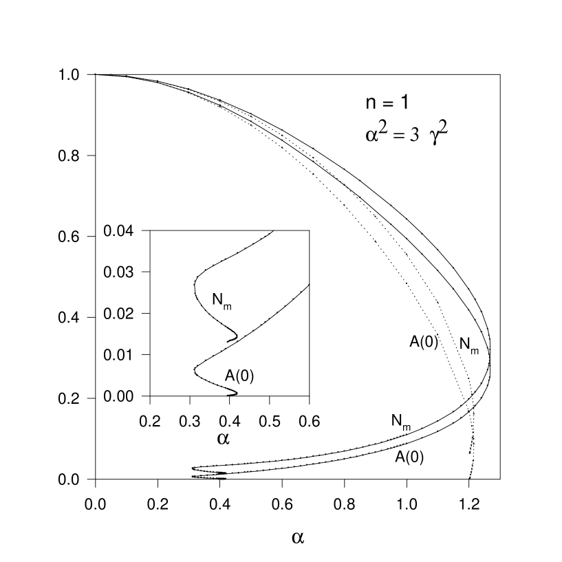
Figure 1: The values of the minimum of the metric function $N$, $N_{m}$, and of the metric function $A$ at the origin, $A(0)$, are shown as a function of $\alpha$ for the $n=1$ solutions in the Volkov limit $\alpha^{2}=3\gamma^{2}$. The solid and dashed lined curves denote the values obtained in the model studied here and the one studied in [11], respectively.

Volkov observed a spiraling behaviour of the parameters for the EYM vortices. As expected and shown in Fig. 1, we observe this feature as well. Our numerical results suggest that a number of branches exist, on which the minimum of the metric function $N$, $N_{m}$, and the value of the metric function $A$ at the origin, $A(0)$, monotonically decrease. In the limit of critical coupling, the $rr$-component of the corresponding $5$-dimensional metric tensor, expressed in $4$ dimensions through the function $g(x):=e^{2\gamma\psi}N(x)=e^{\frac{2}{\sqrt{3}}\alpha\psi}N(x)$ develops a double zero at a value $x_{m}>0$ of the dimensionless coordinate $x$ [12]. Our numerical results indicate that $x_{m}~{}\epsilon~{}]0:0.082]$.

There exist several local maximal and minimal values of $\alpha$, $\alpha_{max}^{(ij)}$ and $\alpha_{min}^{(ij)}$, respectively. By $\alpha_{max,min}^{(ij)}$ we denote the value of $\alpha$, at which the $i$-th and the $j$-th branch join. We find:

$$\alpha_{max}^{(12)}=1.268\ ,\ \ \alpha_{min}^{(23)}=0.312\ ,\ \ \alpha_{max}^{(34)}=0.419\ ,\ \ \alpha_{min}^{(45)}=0.395\$$ (30)

Apparantly, the difference between $\alpha_{max}$ and its corresponding $\alpha_{min}$ decreases, i.e. the branches get smaller and smaller. We thus conjecture that the limiting solution is reached for a value of $\alpha$ close to $\alpha_{min}^{(45)}=0.395$.

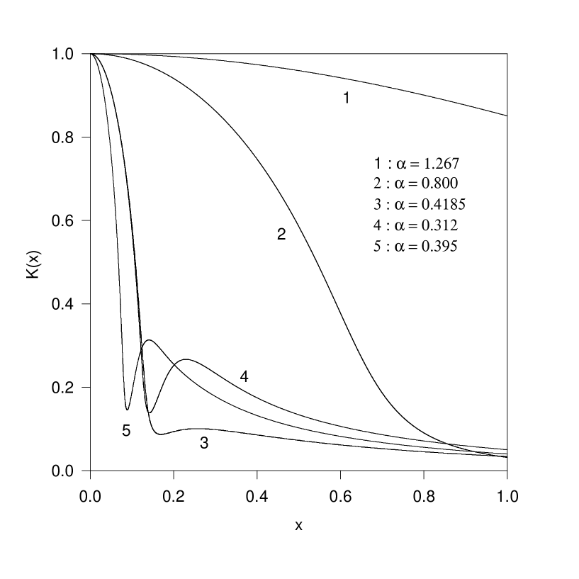
Figure 2: The gauge field function $K(x)$ is shown as function of the dimensionless coordinate $x$ for the $n=1$ solutions in the Volkov limit $\alpha^{2}=3\gamma^{2}$ for the following five values of $\alpha$ : $1:\alpha=1.267$ close to $\alpha_{max}^{(12)}$ , $2:\alpha=0.8$ (second branch), $3:\alpha=0.4185$ (second branch), $4:\alpha_{min}^{(23)}=0.312$ and $5:\alpha_{min}^{(45)}=0.395$.

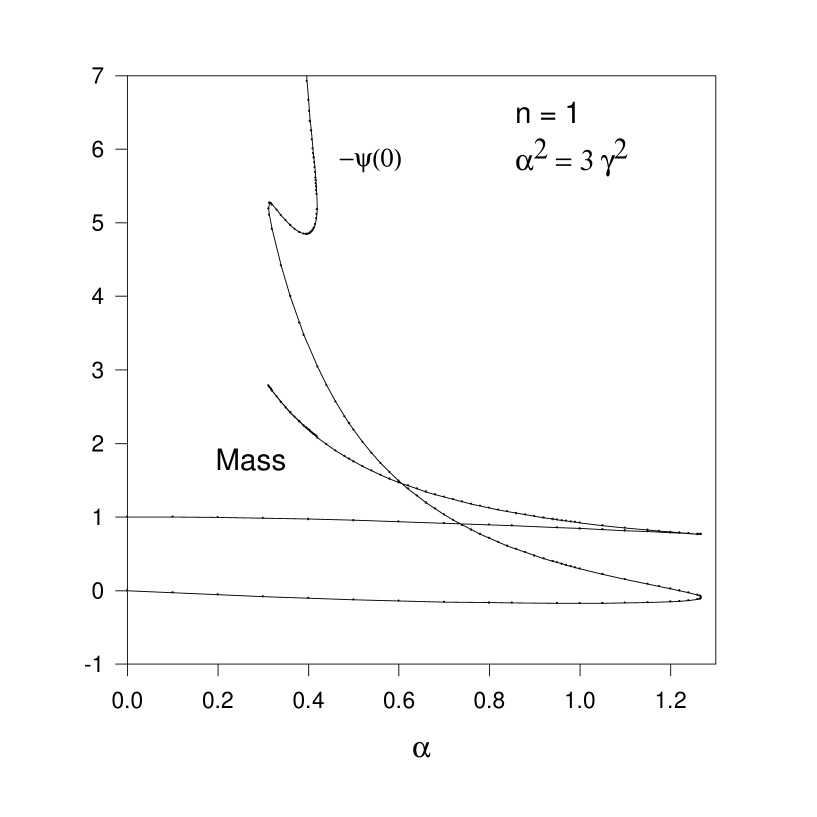
Figure 3: The value of the dilaton function $\psi$ at the origin (multiplied by $-1$), -$\psi(0)$, is shown as function of $\alpha$ for the $n=1$ solutions in the Volkov limit $\alpha^{2}=3\gamma^{2}$. Also shown is the mass of these solutions.

Progressing on the branches, the qualitative behaviour of the functions changes [12]. This is shown for the gauge field function $K(x)$ in Fig. 2. While for all values of $\alpha$ on the first branch (as an example, we show $K(x)$ for $\alpha=1.267$ close to $\alpha_{max}^{(12)}$) and most of the values of $\alpha$ on the second branch (see the profile for $\alpha=0.8$) $K(x)$ decreases monotonically from its value at the origin $K(0)=1$, to its value at infinity $K(\infty)=0$, oscillations of the gauge field start to occur on the second branch for $\alpha\leq 0.4185$. For $\alpha_{min}^{(23)}=0.312$ the local minimum and maximum, respectively, are already quite pronounced, while for $\alpha_{min}^{(45)}=0.395$, the location of both the minimum and maximum has moved to smaller values of $x$. We are convinced that in analogy to [12] the number of oscillations increases when proceeding on further branches. In Fig. 3, we show the value of the dilaton function $\psi$ at the origin (multiplied by $-1$), $-\psi(0)$, and the mass of the solutions on the different branches as functions of $\alpha$. $\psi(0)$ is equal to zero for $\alpha=0$ (since this implies $\gamma=0$), increases to a maximal value of $\psi(0)=0.174$ at $\alpha\approx 1.0$ and from there decreases first to zero at $\alpha=1.220$ on the second branch and further decreases to a minimal value of $\psi(0)=-5.274$ at $\alpha=0.314$ on the third branch. From there it starts to increase to $\psi(0)=-4.847$ at $\alpha=0.395$ and then decreases again to $\psi(0)=-7.164$ at $\alpha_{min}^{(45)}=0.395$.

The function $\psi(x)$ itself decreases monotonically from $\psi(0)$ to its value $\psi(\infty)=0$ for all values of $\gamma$ on the first branch and for $\alpha\leq 1.24$ on the second branch, staying positive for all values of $x$. For $\alpha>1.24$ on the second branch, a minimum (which has negative value) starts to form and dips down deeper to negative values when progressing on the branches. In the limit of critical coupling $\alpha_{cr}$, the dilaton function $\psi_{EMD}$ of the corresponding EMD solution [11]

$$\psi_{EMD}=\frac{\sqrt{3}}{4\alpha_{cr}}\ln(1-\frac{X_{-}}{X})\ ,\ \ \ X_{-}=(\frac{4}{3})^{1/4}$$ (31)

where the dimensionless coordinate $x$ is given in terms of $X$  ,

$$x=\alpha_{cr}X(1-\frac{X_{-}}{X})^{1/4}$$ (32)

is reached for $x\geq x_{m}$, while it stays finite for $x~{}\epsilon~{}[0:x_{m}[$.

It has to be remarked here, though, that in the limit of critical coupling, the gauge and Higgs field functions $K(x)$ and $H(x)$ don’t reach there abelian values $0$ and $1$ at $x=x_{m}$, respectively, but tend to the fixed point described in [12].

The mass of the solution stays close to one on the first branch and increases monotonically on the second branch. On the third and fourth branch it differs only little from the corresponding mass on the second branch and thus the three different branches can barely be distinguished in Fig. 3. In the limit of critical coupling $\alpha_{cr}$, the mass tends to the mass $\frac{\mu_{EMD}}{\alpha^{2}}$ of the corresponding EMD solution:

$$\frac{\mu}{\alpha^{2}}\rightarrow\frac{\mu_{EMD}}{\alpha_{cr}^{2}}=\sqrt{\frac{3}{4}}\frac{1}{\alpha_{cr}}$$ (33)

Let us finally investigate the Einstein-Yang-Mills-Higgs (EYMH) system with the usual coupling of the dilaton considered in [11] in the Volkov limit $\alpha^{2}=3\gamma^{2}$ . This model doesn’t contain the prefactor of the covariant derivative involving the dilaton studied here. In the BPS limit ($\beta=0$), the equation for the Higgs field doesn’t involve the dilaton field directly and vice versa, while in the model studied here it does even for $\beta=0$ (see (18) and (19)). In Fig. 1, we show the values of $N_{m}$ and $A(0)$ for the model studied in [11] for the Volkov limit $\alpha^{2}=3\gamma^{2}$. The recalculation of the configurations for this specific relation between $\alpha$ and $\gamma$ exactly confirms the results obtained in [11]. The solutions exist for $\alpha<\alpha_{max}=1.216$, which fulfills the condition (48) of [11]

$$\sqrt{\alpha_{max}^{2}+\gamma^{2}}=\sqrt{\frac{4}{3}}\alpha_{max}\approx 1.4\ .\$$ (34)

From there, on a second branch of solutions, the Einstein-Maxwell-dilaton (EMD) solution is reached at $\alpha_{cr}$ with the minimum of the metric function $N$, $N_{m}$, tending to the value $N(x=0)$ of the corresponding EMD solution [15]:

$$N_{m}\rightarrow N_{EMD}(0)=(\frac{\gamma^{2}}{\alpha^{2}+\gamma^{2}})^{2}=\frac{1}{16}$$ (35)

This is demonstrated in Fig. 1. $A(0)$ decreases to zero, while $N_{m}>0$, indicating that the extremal EMD solutions have a singularity at $x=0$ not hidden by an horizon.

4 Axially symmetric solutions

Since the $n=1$ monopole was shown to be the unique spherically symmetric solution in SU(2) YMH theory [16], we need to impose an axially symmetric Ansatz (or one with even less symmetry) to construct higher winding number solutions. The axially symmetric Ansatz for the metric in isotropic coordinates reads:

$$ds^{2}=-fdt^{2}+\frac{m}{f}\left(d\tilde{r}^{2}+\tilde{r}^{2}d\theta^{2}\right)+\frac{l}{f}\tilde{r}^{2}\sin^{2}\theta d\varphi^{2}\ ,$$ (36)

The functions $f$, $m$ and $l$ now depend on $\tilde{r}$ and $\theta$. If $l=m$ and $f$ only depend on $\tilde{r}$, this metric reduces to the spherically symmetric metric in isotropic coordinates and comparison with the metric in (9) yields the coordinate transformation [17]:

$$\frac{d\tilde{r}}{\tilde{r}}=\frac{1}{\sqrt{N(r)}}\frac{dr}{r}$$ (37)

For the gauge fields we choose the purely magnetic Ansatz [5]:

$${A_{t}}^{a}=0\ ,\ \ \ {A_{\tilde{r}}}^{a}=\frac{H_{1}}{e\tilde{r}}{v_{\varphi}}^{a}\ ,$$ (38)

$${A_{\theta}}^{a}=\frac{1-H_{2}}{e}{v_{\varphi}}^{a}\ ,\ \ \ \ {A_{\varphi}}^{a}=-\frac{n}{e}\sin\theta\left(H_{3}{v_{\tilde{r}}}^{a}+(1-H_{4}){v_{\theta}}^{a}\right)\ .$$ (39)

while for the Higgs field, the Ansatz reads [5, 18]

$${\Phi}^{a}=v(\Phi_{1}{v_{\tilde{r}}}^{a}+\Phi_{2}{v_{\theta}}^{a})\ .$$ (40)

The vectors $\vec{v}_{\tilde{r}}$,$\vec{v}_{\theta}$ and $\vec{v}_{\varphi}$ are given by:

$$\vec{v}_{\tilde{r}} = (\sin\theta\cos n\varphi,\sin\theta\sin n\varphi,\cos\theta)\ ,$$

$$\vec{v}_{\theta} = (\cos\theta\cos n\varphi,\cos\theta\sin n\varphi,-\sin\theta)\ ,$$

$$\vec{v}_{\varphi} = (-\sin n\varphi,\cos n\varphi,0)\ .$$ (41)

The dilaton field $\Psi$ now depends on $\tilde{r}$ and $\theta$ [8]:

$$\Psi=\Psi(\tilde{r},\theta)$$ (42)

For $H_{1}=H_{3}=\Phi_{2}=0$, $H_{2}=H_{4}=K(\tilde{r})$, $\Phi_{1}=H(\tilde{r})$, $\Psi=\Psi(\tilde{r})$ and $n=1$, this Ansatz reduces to the spherically symmetric Ansatz in isotropic coordinates.

The Euler-Larange equations arise by varying the Lagrangian with respect to the matter fields, while we use the following combinations of the Einstein equations [19]

$$g_{\tilde{r}\tilde{r}}(G^{\mu}_{\mu}-2G^{t}_{t})=16\pi G\frac{m}{f}(L_{M}+g^{tt}\frac{\partial L_{M}}{\partial g^{tt}}-g^{\tilde{r}\tilde{r}}\frac{\partial L_{M}}{\partial g^{\tilde{r}\tilde{r}}}-g^{\theta\theta}\frac{\partial L_{M}}{\partial g^{\theta\theta}}-g^{\varphi\varphi}\frac{\partial L_{M}}{\partial g^{\varphi\varphi}})$$ (43)

$$g_{\tilde{r}\tilde{r}}(G^{\tilde{r}}_{\tilde{r}}+G^{\varphi}_{\varphi})=16\pi G\frac{m}{f}(L_{M}-g^{\tilde{r}\tilde{r}}\frac{\partial L_{M}}{\partial g^{\tilde{r}\tilde{r}}}-g^{\varphi\varphi}\frac{\partial L_{M}}{\partial g^{\varphi\varphi}})$$ (44)

$$g_{\tilde{r}\tilde{r}}(G^{\tilde{r}}_{\tilde{r}}+G^{\theta}_{\theta})=16\pi G\frac{m}{f}(L_{M}-g^{\tilde{r}\tilde{r}}\frac{\partial L_{M}}{\partial g^{\tilde{r}\tilde{r}}}-g^{\theta\theta}\frac{\partial L_{M}}{\partial g^{\theta\theta}})$$ (45)

to obtain $3$ differential equations for the metric functions $f$, $l$ and $m$, which are diagonal with respect to the set of derivatives ($f_{,\tilde{r},\tilde{r}}$, $m_{,\tilde{r},\tilde{r}}$, $l_{,\tilde{r},\tilde{r}}$, $l_{,\theta,\theta}$, $l_{,\tilde{r},\theta}$). With an analog rescaling as in (15), the set of $10$ partial differential equations again depends only on the three fundamental coupling constants introduced in (16).
At the origin, the boundary conditions read (with $\partial_{\tilde{x}}=\frac{1}{ev}\partial_{\tilde{r}}$):

$$\partial_{\tilde{x}}f(0,\theta)=\partial_{\tilde{x}}l(0,\theta)=\partial_{\tilde{x}}m(0,\theta)=0,\ \ \partial_{\tilde{x}}\psi(0,\theta)=0$$ (46)

$$H_{i}(0,\theta)=0,\ i=1,3,\ \ H_{i}(0,\theta)=1,\ i=2,4,\ \ \phi_{i}(0,\theta)=0,\ i=1,2$$ (47)

At infinity, the requirement for finite energy and asymptotically flat solutions leads to the boundary conditions:

$$f(\infty,\theta)=l(\infty,\theta)=m(\infty,\theta)=1,\ \ \psi(\infty,\theta)=0$$ (48)

$$H_{i}(\infty,\theta)=0,\ i=1,2,3,4,\ \ \phi_{1}(\infty,\theta)=1,\ \ \phi_{2}(\infty,\theta)=0$$ (49)

In addition, boundary conditions on the symmetry axes (the $\rho$- and $z$-axes) have to be fulfilled. On both axes:

$$H_{1}=H_{3}=\phi_{2}=0$$ (50)

and

$$\partial_{\theta}f=\partial_{\theta}m=\partial_{\theta}l=\partial_{\theta}H_{2}=\partial_{\theta}H_{4}=\partial_{\theta}\phi_{1}=\partial_{\theta}\psi=0$$ (51)

4.1 Numerical results

Constructing the axially symmetric solutions numerically [20], we were mainly interested whether bound multimonopoles are possible in this model and if so, how the strength of attraction compares to that in [8].

4.1.1 The $\alpha=0$ limit

Since gravity itself is known to be attractive, we first studied the influence of the dilaton alone. Constructing the $n=2$ solutions, we obtain the same qualitative feature as for the $n=1$ case. The configurations exist for all values of $\gamma$, tending to the vacuum solution $H_{1}=H_{3}=\phi_{1}=\phi_{2}=\psi\equiv 0$, $H_{2}=H_{4}\equiv 1$ for $\gamma\rightarrow\infty$. Again, we find that $\psi(0)\geq 0$ and that the curve for $\psi(0)$, starting from zero at $\gamma=0$, develops a maximum at $\gamma=1.38$ (which coincides with the corresponding value for $n=1$). From there it monotonically decreases to zero for $\gamma\rightarrow\infty$.

In Fig. 4, we show the difference between the mass of the $n=1$ solution and the mass per winding number of the $n=2$ solution $\Delta E=E(n=1)-E(n=2)/2$. The sign of $\Delta E$ indicates whether like charged monopoles attract or repell each other, the modulus of $\Delta E$ indicates the strength of attraction and repulsion, respectively. We find that for all values of $\gamma$ we have studied, the monopoles are in an attractive phase and that with increasing $\gamma$ the strength of attraction grows. For the model studied in [8], the maximal $\Delta E$ was found to be $\Delta E_{max}\approx 0.0082$ at $\gamma=1.2$. From there $\Delta E$ decreases since the spherically as well as the axially symmetric monopoles are tending to an essentially abelian, spherically symmetric solution in the limit of critical coupling. In the model studied here, $\Delta E$ is smaller for the same values of $\gamma$ (e.g. we find that $\Delta E(\gamma=1.2)\approx 0.0069$), but since no critical coupling exists, $\Delta E$ grows with increasing $\gamma$. For e.g. $\gamma=5.0$, we find $\Delta E\approx 0.0167$, which is more that twice the maximal possible value for the model in [8]. For large enough values of $\gamma$, $\Delta E$ should decrease, because both the spherically and axially symmetric solution are tending to the vacuum. Since the absolute value of the mass is decreasing to zero, the same should happen for $\Delta E$.

4.1.2 The Volkov limit $\alpha^{2}=3\gamma^{2}$

Studying the $n=2$ axially symmetric monopoles, we find the same qualitative features as in the spherically symmetric case. We obtain:

$$\alpha_{max}^{(12)}=1.279\ ,\ \ \alpha_{min}^{(23)}=0.295$$ (52)

These values are slightly bigger and smaller, respectively, than the corresponding values for the $n=1$ solution. It has already been observed previously, that the branches for the $n=2$ solutions exist for higher values of the maximal coupling [17]. We find here that an analog holds true for the minimal coupling, namely that the $n=2$ solutions exist for smaller minimal values than in the $n=1$ case.

The behaviour of $\psi(0)$ is completely analog to the $n=1$ case : starting from zero at $\alpha=0$, it increases to a maximal value of $\psi(0)\approx 0.178$ at $\alpha\approx 1.0$, then decreases to zero at $\alpha\approx 1.19$ and reaches $\psi(0)\approx-5.324$ at $\alpha_{min}^{(23)}=0.295$. The dilaton function, which has only a weak angle-dependence, is positive and monotonically decreasing on the first branch and starts to form a negative valued minimum on the second branch. Proceeding on the second branch, the solutions are less and less angle dependent and the maximum of the function $H_{1}$, $H_{3}$ and $\Phi_{2}$ decreases. We didn’t manage to construct further branches with our numerical routine (since these branches are rather small), but believe that in analogy to the $n=1$ solutions, the $n=2$ solutions develop a double zero, which is now (because of the choice of isotropic coordinates) located at $\tilde{x}=0$.

Comparing $\Delta E$ for the model studied here and for that in [8], we find that the different values don’t deviate very much from each other. However, in the model studied in [8] the parameter space, in which solutions exist, is limited by $\sqrt{\alpha^{2}+\gamma^{2}}\approx 1.4$. This means that in the Volkov limit solutions only exist for $\alpha\leq\alpha_{max}\approx 1.21$. Here, the solutions exist for bigger values of $\alpha=\sqrt{3}\gamma$ and thus the maximum of $\Delta E$ is slightly bigger with $\Delta E_{max}\approx 0.011$. This is reached on the first branch of solutions as demonstrated in Fig. 4. The second branch starts from a value of $\Delta E$ well below the corresponding one on the first branch and from there decreases. For all values of $\gamma=\frac{\alpha}{\sqrt{3}}$, the value of $\Delta E$ on the first branch exceeds the value of $\Delta E$ on the second branch.

5 Conclusion and Summary

We have studied spherically and axially symmetric solutions of SU(2) EYMHD theory. The specific coupling between the dilaton and the Higgs field in this model arises from a ($4+1$)-dimensional EYM model studied recently in [12]. We find that in the flat space limit ($\alpha=0$), the solutions exist for all values of $\gamma$ tending to the vacuum solution for $\gamma\rightarrow\infty$. This contrasts to the situation in the usual YMHD model studied in [7], where the solutions only exist for $\gamma\leq\gamma_{max}$ tending to an abelian solution in the limit of critical coupling $\gamma_{cr}$. In both models, the dilatonic monopoles are in an attractive phase. Since no critical coupling exists in the model studied here, much stronger bound monopoles are possible.

Apparently, unlike the YMHD model with the usual coupling, the YMHD system studied here doesn’t have analog features than the EYMH system. Moreover, the relation between the $tt$-component of the metric and the dilaton found in [11], doesn’t exist

When in addition gravity is coupled, our equations agree with those in [12] for a specific relation between the gravitational coupling $\alpha$ and the dilaton coupling $\gamma$, namely $\alpha^{2}=3\gamma^{2}$. Studying the spherically and axially symmetric solutions of these equations in this limit, we observe the same spiraling behaviour of the parameters found in [12]. Several branches exist differing from the situation in the model with the usual dilaton coupling studied in [11], where maximally two branches exist. Like in [8] the dilatonic monopoles can form bound multimonopole states.

In [11], non-abelian black holes of the EYMHD model were studied giving further evidence that the ”No-hair” conjecture doesn’t hold in models involving non-abelian fields. It would be interesting to construct the analogs in this system, especially the axially symmetric non-abelian black holes. Their existence would show that Israel’s theorem cannot be extended to EYMHD theory, like it has previously been observed in EYMH theory [17].

Finally, since in the low energy effective action of string theory, further corrections to the equations of standard physics, such as higher order corrections to gravity in form of Gauss-Bonnet terms or new fields like the axion field arise, it would be interesting to study their influence on the solutions constructed here.

Acknowledgements B. H. was supported by the EPSRC.

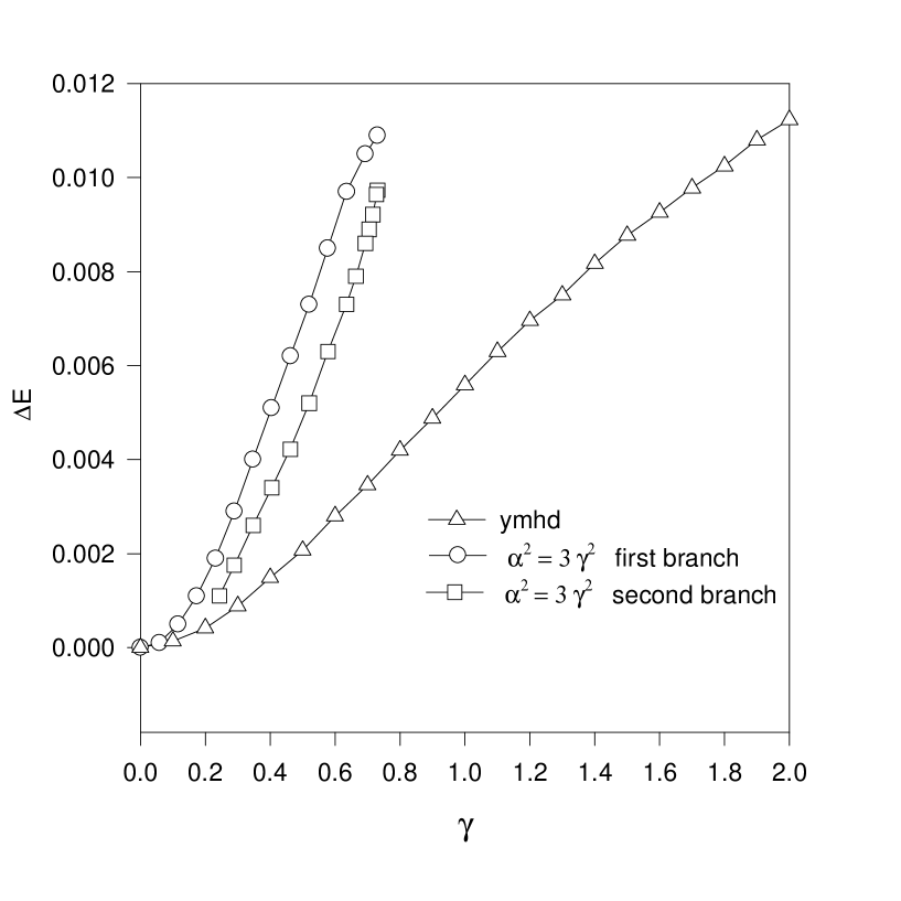
Figure 4: The difference between the mass of the $n=1$ solution and the mass per winding number of the $n=2$ solution $\Delta E=E(n=1)-E(n=2)/2$ is shown as function of $\gamma$ for the first (circles) and second (squares) branch arising in the EYMHD system in the Volkov limit $\alpha^{2}=3\gamma^{2}$. Also shown is $\Delta E$ for the YMHD solutions (triangles). Note that for the EYMHD solutions, the $\gamma$-axis represents a rescaled $\alpha$-axis.

References

- [1] T. Kaluza, Sitzungsber. Preuss. Akad. Wiss. Berlin (1921); O. Klein, Z. Phys. 37 (1926), 895.
- [2] G. Gibbons and K. Maeda, Nucl. Phys. B298 (1988), 741; D. Garfinkle, G. Horowitz and A. Strominger, Phys. Rev. D43 (1991), 371.
-
[3]
G. ‘t Hooft,
Nucl. Phys. B79 (1974), 276;
A. M. Polyakov, JETP Lett. 20 (1974), 194. - [4] R. S. Ward, Commun. Math. Phys. 79 (1981), 317.
- [5] C. Rebbi and P. Rossi, Phys. Rev. D22 (1980), 2010.
- [6] P. Forgacs, Z. Horvath and L. Palla, Phys. Lett. B99 (1981) 232; Erratum-ibid B101 (1981), 457.
- [7] P. Forgacs and J. Gyueruesi, Phys. Lett. B366 (1996), 205.
- [8] Y. Brihaye and B. Hartmann, Phys. Lett. B., in press, hep-th/0110080.
-
[9]
K. Lee, V.P. Nair and E.J. Weinberg,
Phys. Rev. D45 (1992), 2751;
P. Breitenlohner, P. Forgacs and D. Maison, Nucl. Phys. B383 (1992), 357;
P. Breitenlohner, P. Forgacs and D. Maison, Nucl. Phys. B442 (1995), 126. - [10] B. Hartmann, B. Kleihaus and J. Kunz, Phys. Rev. Lett. 86 (2001), 1422.
- [11] Y. Brihaye, B. Hartmann and J. Kunz, Phys. Rev. D65 (2002), 024019.
- [12] M. S. Volkov, Phys. Lett. B524 (2002), 369.
- [13] To integrate the equations, we used the differential equation solver COLSYS which involves a Newton-Raphson method [14].
- [14] U. Ascher, J. Christiansen and R. D. Russell, Math. Comput. 33 (1979), 659; ACM Trans. Math. Softw. 7 (1981), 209.
- [15] In [11], eq. (45) contains an error, since an overall square is missing on the rhs of that equation.
- [16] B. Bogomol’nyi, Sov. J. Nucl. Phys. 24 (1976), 449.
- [17] B. Hartmann, B. Kleihaus and J. Kunz, Phys. Rev. D65 (2002), 024027.
- [18] B. Kleihaus, J. Kunz and T. Tchrakian, Mod. Phys. Lett. A13 (1998), 2523.
- [19] B. Kleihaus and J. Kunz, Phys. Rev. D57 (1998), 834.
- [20] To solve the set of partial differential equations, we used the numerical routine used and described e.g. in [17].