NTUA–02–2002

hep-th/0202044

Brane Cosmology

E. Papantonopoulos^a

National Technical University of Athens, Physics Department, Zografou Campus, GR 157 80, Athens, Greece.

The aim of these lectures is to give a brief introduction to brane cosmology. After introducing some basic geometrical notions, we discuss the cosmology of a brane universe with matter localized on the brane. Then we introduce an intrinsic curvature scalar term in the bulk action, and analyze the cosmology of this induced gravity. Finally we present the cosmology of a moving brane in the background of other branes, and as a particular example, we discuss the cosmological evolution of a test brane moving in a background of a Type-0 string theory.

Lectures presented at the First Aegean Summer School on Cosmology, Samos, September 2001.

^a e-mail address:lpapa@central.ntua.gr

1 Introduction

Cosmology today is an active field of physical thought and of exiting experimental results. Its main goal is to describe the evolution of our universe from some initial time to its present form. One of its outstanding successes is the precise and detailed description of the very early stages of the universe evolution. Various experimental results confirmed that inflation describes accurately these early stages of the evolution. Cosmology can also help to understand the large scale structure of our universe as it is viewed today. It can provide convincing arguments why our universe is accelerating and it can explain the anisotropies of the Cosmic Microwave Background data.

The mathematical description of Cosmology is provided by the Einstein equations. A basic ingredient of all cosmological models is the matter content of the theory. Matter enters Einstein equations through the energy momentum tensor. The form of the energy momentum tensor depends on the underlying theory. If the underlying theory is a Gauge Theory, the scalar sector of the theory must be specified and in particular its scalar potential. Nevertheless, most of the successful inflationary models, which rely on a scalar potential, are not the result of an uderlying Gauge Theory, but rather the scalar content is arbitrary fixed by hand.

In String Theory the Einstein equations are part of the theory but the theory itself is consistent only in higher than four dimensions. Then the cosmological evolution of our universe is studied using the effective four dimensional String Theory. In this theory the only scalar available is the dilaton field. The dilaton field appears only through its kinetic term while a dilaton potential is not allowed. To have a dilaton potential with all its cosmological advantages, we must consider $a^{\prime}$ corrections to the String Theory. Because of this String Theory is very restrictive to its cosmological applications.

The introduction of branes into cosmology offered another novel approach to our understanding of the Universe and of its evolution. It was proposed [1] that our observable universe is a three dimensional surface (domain wall , brane ) embedded in a higher dimensional space. In an earlier speculation, motivated by the long standing hierarchy problem, it was proposed [2] that the fundamental Planck scale could be close to the gauge unification scale, at the price of ”large” spatial dimensions, the introduction of which explains the observed weakness of gravity at long distances. In a similar scenario [3], our observed world is embedded in a five-dimensional bulk, which is strongly curved. This allows the extra dimension not to be very large, and we can perceive gravity as effectively four-dimensional.

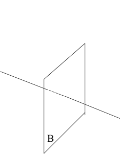
Figure 1: A brane embedded in a five dimensional space.

This idea of a brane universe can naturally be applied to String Theory. In this context, the Standard Model gauge bosons as well as charged matter arise as fluctuations of the D-branes. The universe is living on a collection of coincident branes, while gravity and other universal interactions is living in the bulk space [4].

This new perception of our world had opened new directions in cosmology, but at the same time imposed some new problems. The cosmological evolution of our universe should take place on the brane, but for the whole theory to make sense, the brane should be embedded in a consistent way to a higher dimensional space the bulk. The only physical field in the bulk is the gravitational field, and there are no matter fields. Nevertheless the bulk leaves its imprint on the brane, influencing in this way the cosmological evolution of our universe. In the very early attempts to study the brane cosmology, one of the main problems was, how to get the standard cosmology on the brane.

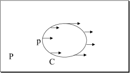
Figure 2: A vector moving around a curve $C$.

In these lectures, which are addressed to the first years graduates students, we will discuss the cosmological evolution of our universe on the brane. Our approach would be more pedagogical, trying to provide the basic ideas of this new cosmological set-up, and more importantly to discuss the mathematical tools necessary for the construction of a brane cosmological model. For this reason will not exhaust all the aspects of brane cosmology. For us, to simplify things, a brane is a three dimensional surface which is embedded in a higher dimensional space which has only one extra dimension, parametrized by the coordinate $y$, as it is shown in Fig.1.

The lectures are organized as follows. In section two after an elementary geometrical description of the extrinsic curvature, we will describe in some detail the way we embed a D-dimensional surface in a D+1-dimensional bulk. We believe that understanding this procedure is crucial for being able to construct a brane cosmological model. In section three we will present the Einstein equations on the brane and we will solve them for matter localized on the brane. Then we will discuss the Friedmann-like equation we get on the brane and the ways we can recover the standard cosmology. In section four we will see what kind of cosmology we get if we introduce in the bulk action a four-dimensional curvature scalar. In section five we will consider a brane moving in the gravitational field of other branes, and we will discuss the cosmological evolution of a test brane moving in the background of a type-0 string theory. Finally in the last section we will summarize the basic ideas and results of brane cosmology.

2 A Surface $\Sigma$ embedded in a D-dimensional Manifold $M$

2.1 Elementary Geometry

To understand the procedure of the embedding of a surface $\Sigma$ in a higher dimensional manifold, we need the notion of the extrinsic curvature . We start by explaining the notion of the curvature [5].

If you have a plane $P$ and a curve $C$ on it, then any vector starting from the point $p$ and moving along the curve $C$ it will come at the same point p with the same direction as it started as shown in Fig.2. However, if the surface was a three dimensional sphere, and a vector starting from $p$ is moving along $C$, will come back on $p$, having different direction from the direction it started with, as shown in Fig.3.

These two examples give the notion of the curvature . The two dimensional surface is flat, while the three dimensional surface is curved. Having in mind Fig.2 and Fig.3 we can say that a space is curved if and only if some initially parallel geodesics fail to remain parallel. We remind to the reader that a geodesic is a curve whose tangent is parallel-transported along itself, that is a ”straightest possible” curve.

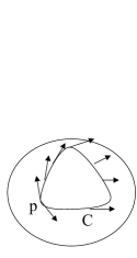
Figure 3: A vector moving around a curve $C$ on a sphere.

We can define the notion of the parallel transport of a vector along a curve $C$ with a tangent vector $t^{a}$, using the derivative operator $\nabla_{a}$. A vector $v^{a}$ given at each point on the curve is said to be parallely transported, as one moves along the curve, if the equation

$$t^{a}\nabla_{a}v^{b}$$ (1)

is satisfied along the curve. Consider a point $q$ on $\Sigma$ with a normal vector $n^{a}$. If I parallel transport the vector $n^{a}$ to a point $p$, then it will be the dashed lines. The failure of this vector to coincide with the vector $n^{a}$ at $p$ corresponds intuitively to the bending of $\Sigma$ in the space time in which is embedded (Fig.4). This is expressed by the extrinsic curvature

$$K_{ab}=h^{c}_{a}\nabla_{c}n_{b}$$ (2)

where $h_{ab}$ the metric on $\Sigma$.

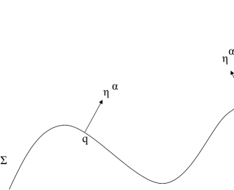
Figure 4: The notion of extrinsic curvature.

2.2 The Embedding Procedure

Imagine now that we have a surface $\Sigma$ (Known also as a domain wall or brane) embedded in a D-dimensional Manifold $M$ [6]. Assume that M splits in two parts $M_{\pm}$. We demand the metric to be continuous everywhere and the derivatives of the metric to be continuous everywhere except on $\Sigma$. The Einstein-Hilbert action on $M$ is

$$S_{EH}=-\frac{1}{2}\int d^{D}x\sqrt{-g}R$$ (3)

where $g_{MN}$ is the metric on $M$, with M,N=1,…,D. We define the induced metric on $\Sigma$ as

$$h_{MN}=g_{MN}-n_{M}n_{N}$$ (4)

where $n_{M}$ is the unit normal vector into $M\pm$. We vary the action (3) in $M\pm$ and we get

$$\delta S_{EH}=-\frac{1}{2}\int_{\Sigma\pm}d^{D-1}\sqrt{-h}g^{MN}n^{p}(\nabla_{M}\delta g_{NP}-\nabla_{P}\delta g_{MN})$$ (5)

If we replace $g^{MN}=h^{MN}+n^{M}n^{N}$ in (5) we get

$$\delta S_{EH}=-\frac{1}{2}\int_{\Sigma\pm}d^{D-1}\sqrt{-h}h^{MN}n^{p}(\nabla_{M}\delta g_{NP}-\nabla_{P}\delta g_{MN})$$ (6)

Recognize the term $(\nabla_{M}\delta g_{NP}-\nabla_{P}\delta g_{MN})$ as the discontinuity of the derivative of the metric across the surface. We do not like discontinuities so we introduce on both side of the surface $\Sigma$, the Gibbons-Hawking boundary term

$$S_{GH}=-\frac{1}{2}\int_{\Sigma\pm}d^{D-1}\sqrt{-h}K$$ (7)

where $k=h^{MN}K_{MN}$ and $K_{MN}$ is the extrinsic curvature defined in (2). If we vary the Gibbons-Hawking term we get as expected

$$\delta S_{GH}=-\frac{1}{2}\int_{\Sigma\pm}d^{D-1}\sqrt{-h}(\delta K-\frac{1}{2}Kh^{MN}\delta g_{MN})$$ (8)

we need the variation of $\delta K$. If we use the variation

$$\delta n_{M}=\frac{1}{2}n_{M}n^{P}n^{Q}\delta g_{PQ}$$ (9)

after some work we get

$$\delta K=-K^{MN}\delta g-h^{MN}n^{P}(\nabla_{M}\delta g_{NP}-\nabla_{P}\delta g_{MN})+\frac{1}{2}Kn^{P}n^{Q}\delta g^{PQ}$$ (10)

We have the variation of both terms $S_{EH}$ and $S_{GH}$ in (6) and (8). Puting everything together we get

$$\delta S_{EH}+\delta S_{GH} = \int d^{D-1}x\sqrt{-h}\Big{(}\frac{1}{2}h^{MN}n^{P}\nabla_{M}g_{NP}+K^{MN}\delta g_{MN}$$

$$- \frac{1}{2}Kn^{M}n^{N}\delta g_{MN}-\frac{1}{2}Kh^{MN}\delta g_{MN}\Big{)}$$

To simplify the above formula imagine a vector $X^{M}$ tangential to $\Sigma\pm$, then

$$\nabla_{M}X^{M}=h^{MN}\nabla_{M}X_{N}+n^{M}n^{N}\nabla_{M}X_{N}$$ (12)

Define the derivative operator $\widetilde{\nabla}$ on $\Sigma$ from

$$\widetilde{\nabla}_{R}X^{M}=h^{M}_{P}h^{Q}_{R}X^{P}$$ (13)

then, using (12) and (13) we have

$$\nabla_{M}X^{M}=\widetilde{\nabla}_{M}X^{M}-X^{M}n^{N}\nabla_{N}X_{M}$$ (14)

and

$$h^{MN}n^{P}\nabla_{M}\delta g_{NP}=\nabla_{M}(h^{MN}n^{P}\delta g_{NP})-\delta g_{NP}\nabla_{M}(h^{MN}n^{P})$$ (15)

If we use the definition of extrinsic curvature $K_{MN}$ from (2) we get

$$h^{MN}n^{P}\nabla_{M}\delta g_{NP}=\nabla_{M}(h^{MN}n^{P}\delta g_{NP})+Kn^{M}n_{N}\delta g_{MN}-K^{MN}\delta g_{MN}$$ (16)

If we substitute (16) in (2.2) and integrate out the total derivative term we get our final result

$$\delta S_{EH}+\delta S_{GH}=\frac{1}{2}\int_{\Sigma\pm}d^{D-1}x\sqrt{-h}(K^{MN}-Kh^{MN})\delta g_{MN}$$ (17)

Therefore what we have done is that starting with the Einstein-Hilbert action, we were forced to introduce the Gibbons-Hawking term, to cancel the discontinuities and the variation of both terms is expressed in terms of the extrinsic curvature and its trace.

2.3 The Israel Matching Conditions

Relation (17) is therefore the result of the embedded surface $\Sigma$ into $M$, a pure geometrical process. Now we can put some dynamics on the surface assuming that there is matter on the surface with an action of the form

$$S_{M}=\int_{\Sigma\pm}d^{D-1}x\sqrt{-h}L_{matter}$$ (18)

where $L_{matter}$ represents the matter on the brane. Then, the variation of (18) gives

$$\delta S_{M}=\int_{\Sigma\pm}d^{D-1}x\sqrt{-h}T^{MN}\delta g_{MN}$$ (19)

where $T^{MN}\equiv-\frac{2}{\sqrt{-h}}\frac{\delta S_{M}}{\delta h_{MN}}$ is the energy momentum tensor of the brane. Now, if we demand the variation of the whole action

$$\delta S=\delta S_{EH}+\delta S_{GH}+\delta S_{M}$$ (20)

to be zero, using (17) and (19) we get the Israel Matching Conditions [7]

$$\Big{\{}K_{MN}-Kh_{MN}\Big{\}}=-T_{MN}$$ (21)

where the curly brackets denote summation over both sides of $\Sigma$. This relation is central for constructing any brane cosmological model. In some way it supplements the Einstein Equations in such a way as to make them consistent on the brane.

3 Brane Cosmology in 5-dimensional Spacetime

3.1 The Einstein Equations on the Brane

The most general action describing a three-dimensional brane in a five-dimensional spacetime is [8]

$$S_{(5)} = \frac{1}{2k^{2}_{5}}\int_{M}d^{5}x\sqrt{-g}\Big{\{}^{(5)}R-2\Lambda_{5}\Big{\}}+\frac{1}{2k^{2}_{4}}\int_{\Sigma}d^{4}x\sqrt{-g}\Big{\{}^{(4)}R-2\Lambda_{4}\Big{\}}$$ (22)

$$+ \int_{M}d^{5}x\sqrt{-g}L^{mat}_{5}+\int_{\Sigma}d^{4}x\sqrt{-g}L^{mat}_{4}$$

where $\Lambda_{5}$ and $\Lambda_{4}$ are the cosmological constants of the bulk and brane respectively, and $L^{mat}_{5}$, $L^{mat}_{4}$ are their matter content. From the dimensionful constants $k^{2}_{5}$, $k^{2}_{4}$ the Planck masses $M_{5}$, $M_{4}$ are defined as

$$k^{2}_{5} = 8\pi G_{(5)}=M^{-3}_{5}$$

$$k^{2}_{4} = 8\pi G_{(4)}=M^{-2}_{4}$$ (23)

We will derive the Einstein equations for the simplified action

$$S_{(5)}=\frac{1}{2k^{2}_{(5)}}\int_{M}d^{5}x\sqrt{-g}^{(5)}R+\int_{M}d^{5}x\sqrt{-g}L^{mat}_{5}$$ (24)

which is historically the first action considered [9], and we will leave for later the general case. We will consider a metric of the form

$$ds^{2}=g_{MN}dx^{M}dx^{N}=g_{\mu\nu}dx^{\mu}dx^{\nu}+b^{2}dy^{2}$$ (25)

where $y$ paramertizes the fifth dimension. We will assume that our four dimensional surface is sited at $y=0$. We allow a time dependence of the fields so our metric becomes

$$ds^{2}=-n^{2}(t,y)dt^{2}+a^{2}(t,y)\delta_{ij}dx^{i}dx^{j}+b^{2}(t,y)dy^{2}$$ (26)

Note that we take for simplicity flat metric for the ordinary spatial dimensions. For the matter content of the action (24) we assume that matter is confined on both, brane and bulk. Then, the energy momentum tensor derived from (24) can be decomposed into

$$T^{M}_{~{}~{}N}=T^{M}_{~{}~{}N}\Big{|}_{bulk}+T^{M}_{~{}~{}N}\Big{|}_{brane}$$ (27)

For the matter on the brane we consider perfect fluid with

$$T^{M}_{~{}~{}N}\Big{|}_{brane}=\frac{\delta(y)}{b}diag(-\rho,p,p,p,,0)$$ (28)

What we want now is to study the dynamics of the metric $g_{\mu\nu}(t,0)$. For this, we have to solve the 5-dimensional Einstein equations

$$G_{MN}=k^{2}_{5}T_{MN}$$ (29)

Inserting (26) in (29) we get

$$G_{00} = 3\Big{\{}\frac{\dot{a}}{a}(\frac{\dot{a}}{a}+\frac{\dot{b}}{b})-\frac{n^{2}}{b^{2}}\Big{(}\frac{a^{{}^{\prime\prime}}}{a}+\frac{a^{{}^{\prime}}}{a}(\frac{a^{{}^{\prime}}}{a}-\frac{b^{{}^{\prime}}}{b})\Big{)}\Big{\}}$$

$$G_{ij} = \frac{a^{2}}{b^{2}}\delta_{ij}\Big{\{}\frac{a^{{}^{\prime}}}{a}(\frac{a^{{}^{\prime}}}{a}+2\frac{n^{{}^{\prime}}}{n})-\frac{b^{{}^{\prime}}}{b}(\frac{n^{{}^{\prime}}}{n}+2\frac{a^{{}^{\prime}}}{a})+2\frac{a^{{}^{\prime\prime}}}{a}+\frac{n^{{}^{\prime\prime}}}{n}\Big{\}}$$

$$+ \frac{a^{{}^{\prime\prime}}}{n^{2}}\delta_{ij}\Big{\{}\frac{\dot{a}}{a}(-\frac{\dot{a}}{a}+2\frac{\dot{n}}{n})+\frac{\dot{b}}{b}(-2\frac{\dot{a}}{a}+\frac{\dot{n}}{n})-2\frac{\ddot{a}}{a}-\frac{\ddot{b}}{b}\Big{\}}$$

$$G_{05} = 3(\frac{n{{}^{\prime}}}{n}\frac{\dot{a}}{a}+\frac{a^{{}^{\prime}}}{a}\frac{\dot{b}}{b}-\frac{\dot{a}^{{}^{\prime}}}{a})$$

$$G_{55} = 3\Big{\{}\frac{a^{{}^{\prime}}}{a}(\frac{a^{{}^{\prime}}}{a}+\frac{n^{{}^{\prime}}}{n})-\frac{b^{2}}{n^{2}}\Big{(}\frac{\dot{a}}{a}(\frac{\dot{a}}{a}-\frac{\dot{n}}{n})+\frac{\ddot{a}}{a}\Big{)}\Big{\}}$$ (30)

We are looking for solutions of the Einstein equations (29) near or in the vicinity of $y=0$. At the point $y=0$, where the brane is situated, we must take under consideration the Israel Boundary Conditions. We can use relations (21) to calculate them or follow an easier way [9]. We require that the derivatives of the metric with respect to $y$, to be discontinuous at $y=0$. This means that in the second derivatives of the quantities $a$ and $n$ a distributional term will appear which will have the form $[a^{{}^{\prime}}]\delta(y)$ or $[n^{{}^{\prime}}]\delta(y)$ with

$$[a^{{}^{\prime}}]=a^{{}^{\prime}}(0^{+})-a^{{}^{\prime}}(0^{-})$$ (31)

$$[n^{{}^{\prime}}]=n^{{}^{\prime}}(0^{+})-n^{{}^{\prime}}(0^{-})$$ (32)

We can calculate the quantities (31) and (32) using equations (3.1) and the energy-momentum tensor (28)

$$\frac{[a^{{}^{\prime}}]}{a_{0}b_{0}} = -\frac{k^{2}_{(5)}}{3}\rho$$

$$\frac{[n^{{}^{\prime}}]}{n_{0}b_{0}} = \frac{k^{2}_{(5)}}{3}(3p+2\rho)$$ (33)

where $a_{0}=a(t,0)$ and $b_{0}=b(t,0)$ and we have set n(t,0)=1. If we use a reflection symmetry $y\longrightarrow-y$ the $(55)$ component of the Einstein equations (29) with the use of (28) and (3.1) becomes

$$\frac{\dot{a}^{2}_{0}}{a^{2}_{0}}+\frac{\ddot{a}_{0}}{a_{0}}=-\frac{k^{4}_{(5)}}{36}\rho(\rho+3p)-k^{2}_{(5)}\frac{T_{55}}{3b^{2}_{0}}$$ (34)

This is our cosmological Einstein equation which governs the cosmological evolution of our brane universe .

3.2 Cosmology on the Brane

Define the Hubble parameter from $H=\frac{\dot{a}_{0}}{a_{0}}$. Then equation (34) becomes

$$2H^{2}+\dot{H}=-\frac{k^{4}_{(5)}}{36}\rho(\rho+3p)-k^{2}_{(5)}\frac{T_{55}}{3b^{2}_{0}}$$ (35)

If one compares equation (35) with usual Friedmann equation, one can see that energy density enters the equation quadratically, in contrast with the usual linear dependence. Another novel feature of equation (35) is that the cosmological evolution depends on the five-dimensional Newton’s constant and not on the brane Newton’s constant.

To have a feeling of what kind of cosmological evolution we get, we consider the Bianchi identity $\nabla_{M}G^{M}_{~{}N}=0$. Then using the Einstein equation (29) and the energy momentum tensor on the brane from (28), we get

$$\dot{\rho}+3(\rho+p)\frac{\dot{a}_{0}}{a_{0}}=0$$ (36)

which is the usual energy density conservation. If we take for the equation of state $p=w\rho$, then the above equation gives for the energy density the usual relation

$$\rho\prec a_{0}e^{-3(1+w)}$$ (37)

If we look for power law solutions however, $a_{0}(t)\prec t^{q}$ equation (35) gives

$$q=\frac{1}{3(1+w)}$$ (38)

which comparing with $q_{standard}=\frac{2}{3(1+w)}$ gives slower expansion.

If we add a cosmological constant in the bulk, then a solution of the Einstein equation (29) can be obtained, in which the universe starts with a non conventional phase and then enters the standard cosmological phase [10, 11, 12].

4 Induced Gravity on the Brane

The effective Einstein equations on the brane which we discussed in section (3.1) were generalized in [13], where matter confined on the brane was taken under consideration. However, a more fundamental description of the physics that produces the brane could include [14] higher order terms in a derivative expansion of the effective action, such as a term for the scalar curvature of the brane, and higher powers of curvature tensors on the brane. In [15, 16] it was observed that the localized matter fields on the brane (which couple to bulk gravitons) can generate via quantum loops a localized four-dimensional worldvolume kinetic term for gravitons. That is to say, four-dimensional gravity is induced from the bulk gravity to the brane worldvolume by the matter fields confined to the brane. We will therefore include the scalar curvature term in our action and we will discuss what is the effect of this term to cosmology.

Our theory is described then by the full action (22). Using relations (3.1) we define a distance scale

$$r_{c}\equiv\frac{\kappa_{5}^{2}}{\kappa_{4}^{2}}=\frac{M_{4}^{2}}{M_{5}^{3}}\,.$$ (39)

Varying (22) with respect to the bulk metric $g_{MN}$, we obtain the equations

$${}^{(5)}G_{MN}=-\Lambda_{5}g_{MN}+\kappa_{5}^{2}\,(^{(5)}T_{MN}+\,^{(loc)}T_{MN}\,\delta(y))\,,$$ (40)

where

$${}^{(loc)}T_{MN}\equiv-\frac{1}{\kappa_{4}^{2}}\,\sqrt{\frac{{}^{(4)}g}{{}^{(5)}g}}\,\,\Big{(}^{(4)}G_{AB}-\kappa_{4}^{2}\,{}^{(4)}T_{MN}+\Lambda_{4}g_{MN}\Big{)}$$ (41)

is the localized energy-momentum tensor of the brane. ${}^{(5)}G_{MN}$, ${}^{(4)}G_{MN}$ denote the Einstein tensors constructed from the bulk and the brane metrics respectively. Clearly, ${}^{(4)}G_{MN}$ acts as an additional source term for the brane through ${}^{(loc)}T_{MN}$.

It is obvious that the additional source term on the brane will modify the Israel Boundary Conditions (21). The modified conditions are

$$[K_{~{}\nu}^{\mu}]=-\kappa_{5}^{2}\,b_{o}\,\left({}^{(loc)}T_{~{}\nu}^{\mu}-\frac{{}^{(loc)}T}{3}\delta_{\nu}^{\mu}\right)\,,$$ (42)

where the bracket means discontinuity of the extrinsic curvature $K_{\mu\nu}=\frac{1}{2b}\partial_{y}g_{\mu\nu}$ across $y=0$, and $b_{o}=b(y=0)$. A $\mathbf{Z}_{2}$ symmetry on reflection around the brane is understood throughout.

Using equations (40) and (42) we can derive the four-dimensional Einstein equations on the brane [8]. They are

$$^{(4)}G^{\mu}_{~{}\nu}=k^{2}_{(4)}~{}^{(4)}T^{\mu}_{~{}\nu}-\Lambda_{(4)}\delta^{\mu}_{~{}\nu}-a\Big{(}L^{\mu}_{~{}\nu}+\frac{L}{2}+\frac{3}{2}a\Big{)}\delta^{\mu}_{~{}\nu}$$ (43)

where $\alpha\equiv 2/r_{c}$, while the quantities $L^{\mu}_{~{}\nu}$ are related to the matter content of the theory through the equation

$$L_{\lambda}^{\mu}L_{\nu}^{\lambda}-\frac{L^{2}}{4}\,\delta_{\nu}^{\mu}=\widetilde{T}_{\nu}^{\mu}-\frac{1}{4}\Big{(}3\alpha^{2}+2\widetilde{T}_{\lambda}^{\lambda}\Big{)}\delta_{\nu}^{\mu}\,,$$ (44)

and $L\equiv L^{\mu}_{\mu}$. The quantities $\widetilde{T}^{\mu}_{\nu}$ are given by the expression

$$\widetilde{T}_{\nu}^{\mu} = \Big{(}\Lambda_{4}-\frac{1}{2}\,\Lambda_{5}\Big{)}\delta_{\nu}^{\mu}-\kappa_{4}^{2}\,{}^{(4)}T_{\nu}^{\mu}+$$ (46)

$$+\frac{2}{3}\,\kappa_{5}^{2}\,\Big{(}\,^{(5)}\overline{T}\,_{\nu}^{\mu}+\Big{(}\,^{(5)}\overline{T}\,_{y}^{y}-\frac{{}^{(5)}\overline{T}}{4}\Big{)}\,\delta_{\nu}^{\mu}\Big{)}-\overline{\textsf{E}}^{\,\mu}_{\,\nu}\,.$$

Bars over ${}^{(5)}T^{\mu}_{\nu}$ and the electric part  $\textsf{E}^{\,{}^{\mu}}_{\,\nu}=C^{\mu}_{M\nu N}n^{M}n^{N}$ of the Weyl tensor $C^{M}_{NPR}$ mean that the quantities are evaluated at $y=0$. $\overline{\textsf{E}}^{\,\mu}_{\,\nu}$ carries the influence of non-local gravitational degrees of freedom in the bulk onto the brane and makes the brane equations (43) not to be, in general, closed. This means that there are bulk degrees of freedom which cannot be predicted from data available on the brane. One needs to solve the field equations in the bulk in order to determine $\textsf{E}^{\,{}^{\mu}}_{\,\nu}$ on the brane.

4.1 Cosmology on the Brane with a $~{}^{(4)}R$ Term

To get a feeling of what kind of cosmology we get on the brane with an ${}^{(4)}R$ term, we consider the metric of (26). To simplify things we take ${}^{(5)}T_{MN}$ to be just the five-dimensional cosmological constant, while for the matter localized on the brane we take ${}^{(4)}T_{MN}$ to have the usual form of a perfect fluid (relation(28)). The new term that enters here in the calculations is the four-dimensional Einstein tensor $~{}^{(4)}G_{MN}$ which appears in $~{}^{(loc)}T$ (relation (41)). The non vanishing components of $~{}^{(4)}G_{MN}$ can be calculated to be

$$~{}~{}~{}^{(4)}G_{00} = -\frac{3\delta(y)}{k^{2}_{4}b}\Big{\{}\frac{\dot{a}^{2}}{a^{2}}+\frac{n^{2}}{a^{2}}\Big{\}}$$

$${}^{(4)}G_{ij} = -\frac{\delta(y)}{k^{2}_{4}b}\Big{\{}\frac{a^{2}}{n^{2}}\delta_{ij}\Big{(}-\frac{\dot{a}^{2}}{a^{2}}+2\frac{\dot{a}\dot{n}}{an}-2\frac{\ddot{a}}{a}\Big{)}-\delta_{ij}\Big{\}}$$ (47)

Then as in section (3.1) we can calculate the distributional parts of the second derivatives as [17]

$$\frac{[a^{{}^{\prime}}]}{a_{0}b_{0}} = -\frac{k^{2}}{3}\rho+\frac{k^{2}_{5}}{k^{2}_{4}n^{2}_{0}}\Big{\{}\frac{\dot{a_{0}}^{2}}{a^{2}_{0}}+\frac{n^{2}_{0}}{a^{2}_{0}}\Big{\}}$$

$$\frac{[n^{{}^{\prime}}]}{n_{0}b_{0}} = \frac{k^{2}}{3}(3p+2\rho)+\frac{k^{2}_{5}}{k^{2}_{4}n^{2}_{0}}\Big{(}-\frac{\dot{a}^{2}_{0}}{a^{2}_{0}}-2\frac{\dot{a}_{0}\dot{n}_{0}}{a_{0}n_{0}}+2\frac{\ddot{a}_{0}}{a_{0}}-\frac{n^{2}_{0}}{a^{2}_{0}}\Big{)}$$

If we again use a reflection symmetry $y\longrightarrow-y$, then the Einstein equations (40) with the use of (28), (4.1) and (4.1) give our cosmological Einstein equation

$$H^{2}-2\frac{k^{2}_{4}}{k^{2}_{5}}\sqrt{H^{2}+\frac{1}{a^{2}_{0}}}=-\frac{k^{2}}{3}\rho+\frac{1}{a^{2}_{0}}$$ (49)

To compare this equation with the evolution equation (34) we had derived without the $~{}^{(4)}R$ term, we observe that the energy density enters the evolution equation linearly as in the standard cosmology. However the evolution equation (49) is not the standard Friedmann cosmological equation. We can recover the usual Friedmann equation [18], if (neglecting the $\frac{1}{a^{2}_{0}}$ term)

$$H^{-1}\ll\frac{M^{2}_{(4)}}{2M^{3}_{(5)}}$$ (50)

If we use the crossover scale $r_{c}$ of (39) the above relation means that an observer on the brane will see correct Newtonian gravity at Hubble distances shorter than a certain crossover scale, despite the fact that gravity propagates in extra space which was assumed there to be flat with infinite extent; at larger distances, the force becomes higher-dimensional. We can get the same picture if we look at the equation (44). If the crossover scale $r_{c}$ is large, then $\alpha\equiv 2/r_{c}$ is small and the last term in (44) decouples, giving the usual four-dimensional Einstein equations.

5 A brane on a Move

So far the domain walls (branes) were static solutions of the underlying theory, and the cosmological evolution of our universe was due mainly to the time evolution of energy density on the domain wall (brane). In this section we will consider another approach. The cosmological evolution of our universe is due to the motion of our brane-world in the background gravitational field of the bulk [6, 19, 20, 21].

In [6] the motion of a domain wall (brane) in a higher dimensional spacetime was studied. The Israel matching conditions were used to relate the bulk to the domain wall (brane) metric, and some interesting cosmological solutions were found. In [20] a universe three-brane is considered in motion in ten-dimensional space in the presence of a gravitational field of other branes. It was shown that this motion in ambient space induces cosmological expansion (or contraction) on our universe, simulating various kinds of matter. In particular, a D-brane moving in a generic static, spherically symmetric background was considered. As the brane moves in a geodesic, the induced world-volume metric becomes a function of time, so there is a cosmological evolution from the brane point of view. The metric of a three-dimensional brane is parametrized as

$$ds^{2}_{10}=g_{00}(r)dt^{2}+g(r)(d\vec{x})^{2}+g_{rr}(r)dr^{2}+g_{S}(r)d\Omega_{5}$$ (51)

and there is also a dilaton field $\Phi$ as well as a $RR$ background $C(r)=C_{0...3}(r)$ with a self-dual field strength. The action on the brane is given by

$$S = T_{3}~{}\int~{}d^{4}\xi e^{-\Phi}\sqrt{-det(\hat{G}_{\mu\nu}+(2\pi\alpha^{\prime})F_{\mu\nu}-B_{\mu\nu})}$$ (52)

$$+T_{3}~{}\int~{}d^{4}\xi\hat{C}_{4}+anomaly~{}terms$$

The induced metric on the brane is

$$\hat{G}_{\mu\nu}=G_{MN}\frac{\partial x^{M}\partial x^{N}}{\partial\xi^{\mu}\partial\xi^{\nu}}$$ (53)

with similar expressions for $F_{\alpha\beta}$ and $B_{\alpha\beta}$. In the static gauge, using (53) we can calculate the bosonic part of the brane Lagrangian which reads

$$L=\sqrt{A(r)-B(r)\dot{r}^{2}-D(r)h_{ij}\dot{\varphi}^{i}\dot{\varphi}^{j}}-C(r)$$ (54)

where $h_{ij}d\varphi^{i}d\varphi^{j}$ is the line element of the unit five-sphere, and

$$A(r)=g^{3}(r)|g_{00}(r)|e^{-2\Phi},B(r)=g^{3}(r)g_{rr}(r)e^{-2\Phi},D(r)=g^{3}(r)g_{S}(r)e^{-2\Phi}$$ (55)

Demanding conservation of energy $E$ and of total angular momentum $\ell^{2}$ on the brane, the induced four-dimensional metric on the brane is

$$d\hat{s}^{2}=(g_{00}+g_{rr}\dot{r}^{2}+g_{S}h_{ij}\dot{\varphi}^{i}\dot{\varphi}^{j})dt^{2}+g(d\vec{x})^{2}$$ (56)

with

$$\dot{r}^{2}=\frac{A}{B}(1-\frac{A}{(C+E)^{2}}\frac{D+\ell^{2}}{D}),h_{ij}\dot{\varphi}^{i}\dot{\varphi}^{j}=\frac{A^{2}\ell^{2}}{D^{2}(C+E)^{2}}$$ (57)

Using (57), the induced metric becomes

$$d\hat{s}^{2}=-d\eta^{2}+g(r(\eta))(d\vec{x})^{2}$$ (58)

with $\eta$ the cosmic time which is defined by

$$d\eta=\frac{|g_{00}|g^{\frac{3}{2}}e^{-\Phi}}{|C+E|}dt$$ (59)

This equation is the standard form of a flat expanding universe. If we define the scale factor as $\alpha^{2}=g$ then we can calculate the Hubble constant $H=\frac{\dot{\alpha}}{\alpha}$, where dot stands for derivative with respect to cosmic time. Then we can interpret the quantity $(\frac{\dot{\alpha}}{\alpha})^{2}$ as an effective matter density on the brane with the result

$$\frac{8\pi}{3}\rho_{eff}=\frac{(C+E)^{2}g_{S}e^{2\Phi}-|g_{00}|(g_{S}g^{3}+\ell^{2}e^{2\Phi})}{4|g_{00}|g_{rr}g_{S}g^{3}}(\frac{g^{\prime}}{g})^{2}$$ (60)

Therefore the motion of a three-dimensional brane on a general spherically symmetric background had induced on the brane a matter density. As it is obvious from the above relation, the specific form of the background will determine the cosmological evolution on the brane.

We will go to a particular background, that of a Type-0 string, and see what cosmology we get. The action of the Type-0 string is given by [23]

$$S_{10} = ~{}\int~{}d^{10}x\sqrt{-g}\Big{[}e^{-\Phi}\Big{(}R+(\partial_{\mu}\Phi)^{2}-\frac{1}{4}(\partial_{\mu}T)^{2}-\frac{1}{4}m^{2}T^{2}-\frac{1}{12}H_{mnr}H^{mnr}\Big{)}$$ (61)

$$-\frac{1}{2}(1+T+\frac{T^{2}}{2})|F_{5}|^{2}\Big{]}$$

The equations of motion which result from this action are

$$2\nabla^{2}\Phi-4(\nabla_{n}\Phi)^{2}-\frac{1}{2}m^{2}T^{2}=0$$ (62)

$$R_{mn} +2\nabla_{m}\nabla_{n}\Phi-\frac{1}{4}\nabla_{m}T\nabla_{n}T-\frac{1}{4\cdot 4!}e^{2\Phi}f(T)\Big{(}F_{mklpq}F_{n}~{}^{klpq}$$ (63)

$$-\frac{1}{10}G_{mn}F_{sklpq}F^{sklpq}\Big{)}=0$$

$$(-\nabla^{2}+2\nabla^{n}\Phi\nabla_{n}+m^{2})T+\frac{1}{2\cdot 5!}e^{2\Phi}f^{\prime}(T)F_{sklpq}F^{sklpq}=0$$ (64)

$$\nabla_{m}\Big{(}f(T)F^{mnkpq}\Big{)}=0$$ (65)

The tachyon is coupled to the $RR$ field through the function

$$f(T)=1+T+\frac{1}{2}T^{2}$$ (66)

In the background where the tachyon field acquires vacuum expectation value $T_{vac}=-1$, the tachyon function (66) takes the value $f(T_{vac})=\frac{1}{2}$ which guarantee the stability of the theory [24].

The equations (62)-(65) can be solved using the metric (51). Moreover one can find the electrically charged three-brane if the following ansatz for the $RR$ field

$$C_{0123}=A(r),F_{0123r}=A^{\prime}(r)$$ (67)

and a constant value for the dilaton field $\Phi=\Phi_{0}$ is used

$$g_{00}=-H^{-\frac{1}{2}},g(r)=H^{-\frac{1}{2}},g_{S}(r)=H^{\frac{1}{2}}r^{2},g_{rr}(r)=H^{\frac{1}{2}},H=1+\frac{e^{\Phi_{0}}Q}{2r^{4}}$$ (68)

5.1 Cosmology of the Moving Brane

The induced metric on the brane (56) using the background solution (68) is

$$d\hat{s}^{2}=(-H^{-\frac{1}{2}}+H^{\frac{1}{2}}\dot{r}^{2}+H^{\frac{1}{2}}r^{2}h_{ij}\dot{\varphi}^{i}\dot{\varphi}^{j})dt^{2}+H^{-\frac{1}{2}}(d\vec{x})^{2}$$ (69)

From equation (65) the $RR$ field $C=C_{0123}$ using the ansatz (67) becomes

$$C^{~{}^{\prime}}=2Qg^{2}g^{-\frac{5}{2}}_{s}\sqrt{g_{rr}}f^{-1}(T)$$ (70)

where Q is a constant. Using again the solution (68) the $RR$ field can be integrated to give

$$C=e^{-\Phi_{0}}f^{-1}(T)(1+\frac{e^{\Phi_{0}}Q}{2r^{4}})^{-1}+Q_{1}$$ (71)

where $Q_{1}$ is a constant. The effective density on the brane (60), using equation (68) and (70) becomes [22]

$$\frac{8\pi}{3}\rho_{eff}=\frac{1}{4}[(f^{-1}(T)+EHe^{\Phi_{0}})^{2}-(1+\frac{\ell^{2}e^{2\Phi_{0}}}{2}H)]\frac{Q^{2}e^{2\Phi_{0}}}{r^{10}}H^{-\frac{5}{2}}$$ (72)

where the constant $Q_{1}$ was absorbed in a redefinition of the parameter $E$. Identifying $g=\alpha^{2}$ and using $g=H^{-\frac{1}{2}}$ we get from (72)

$$\frac{8\pi}{3}\rho_{eff} = (\frac{2e^{-\Phi_{0}}}{Q})^{\frac{1}{2}}\Big{[}\Big{(}f^{-1}(T)+\frac{Ee^{\Phi_{0}}}{\alpha^{4}}\Big{)}^{2}-\Big{(}1+\frac{\ell^{2}e^{2\Phi_{0}}}{\alpha^{6}}(\frac{2e^{-\Phi_{0}}}{Q})^{\frac{1}{2}}$$ (73)

$$(1-\alpha^{4})^{\frac{1}{2}}\Big{)}\Big{]}(1-\alpha^{4})^{\frac{5}{2}}$$

From the relation $g=H^{-\frac{1}{2}}$ we find

$$r=(\frac{\alpha^{4}}{1-\alpha^{4}})^{\frac{1}{4}}(\frac{Qe^{\Phi_{0}}}{2})^{\frac{1}{4}}$$ (74)

This relation restricts the range of $\alpha$ to $0\leq\alpha<1$, while the range of $r$ is $0\leq r<\infty$. We can calculate the scalar curvature of the four-dimensional universe as

$$R_{brane}=8\pi(4+\alpha\partial_{\alpha})\rho_{eff}$$ (75)

If we use the effective density of (73) it is easy to see that $R_{brane}$ of (75) blows up at $\alpha=0$. On the contrary if $r\rightarrow 0$, then the $ds^{2}_{10}$ of (51) becomes

$$ds^{2}_{10}=\frac{r^{2}}{L}(-dt^{2}+(d\vec{x})^{2})+\frac{L}{r^{2}}dr^{2}+Ld\Omega_{5}$$ (76)

with $L=(\frac{e^{\Phi_{0}}Q}{2})^{\frac{1}{2}}$. This space is a regular $AdS_{5}\times S^{5}$ space.

Therefore the brane develops an initial singularity as it reaches $r=0$, which is a coordinate singularity and otherwise a regular point of the $AdS_{5}$ space. This is another example in Mirage Cosmology [20] where we can understand the initial singularity as the point where the description of our theory breaks down.

If we take $\ell^{2}=0$, set the function $f(T)$ to each minimum value and also taking $\Phi_{0}=0$, the effective density (73) becomes

$$\frac{8\pi}{3}\rho_{eff}=(\frac{2}{Q})^{\frac{1}{2}}\Big{(}(2+\frac{E}{\alpha^{4}})^{2}-1\Big{)}(1-\alpha^{4})^{\frac{5}{2}}$$ (77)

As we can see in the above relation, there is a constant term, coming from the tachyon function $f(T)$. For small $\alpha$ and for some range of the parameters $E$ and $Q$ it gives an inflationary phase to the brane cosmological evolution. In Fig.5 we have plotted $\rho_{eff}$ as a function of $\alpha$ for $Q=2$. Note here that $E$ is constrained from (57) as $C+E\geq 0$. In our case using (71) we get $E\geq-2\alpha^{4}$, therefore $E$ can be as small as we want.

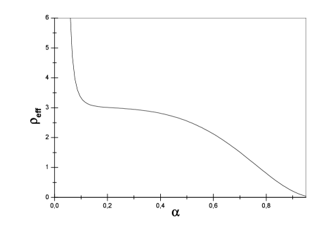
Figure 5: The induced energy density on the brane as a function of the brane scale factor.

The cosmological evolution of a brane universe according to this example is as follows. As the brane moves away from $r=0$ to larger values of $r$, the universe after the inflationary phase enters a radiation dominated epoch because the term $\alpha^{-4}$ takes over in (77). As the cosmic time $\eta$ elapses the $\alpha^{-8}$ term dominates and finally when the brane is far away from $r=0$, the term which is controlled by the angular momentum $\ell^{2}$ gives the main contribution to the effective density. Non zero values of $\ell^{2}$ will give negative values for $\rho_{eff}$. We expect that at later cosmic times there will be other fields, like gauge fields, which will give a different dynamics to the cosmological evolution and eventually cancel the negative matter density.

The above model can be generalized to include a non constant value for the dilaton field. Then using [25] and [26] we can study the cosmological evolution of a brane universe as the brane moves from IR to UV in the background of a type-0 string theory [27, 28, 29, 30].

6 Conclusions

We presented the main ideas and gave the main results of the cosmological evolution of a brane universe. The main new result that brane cosmology offered, is that our universe at some stage of its evolution, passed a cosmological phase which is not described purely by the Friedmann equation of standard cosmology. In the simplest possible brane model, the Hubble parameter scales like the square of the energy density and this results in a slower universe expansion. There were a lot of extensions and modifications of this model, trying to get the standard cosmology but it seems that the universe in a brane world passed from an unconvensional phase at its earliest stages of its cosmological evolution.

The inclusion of an $~{}^{(4)}R$ term in the action, offered a more natural explanation of the brane unconvensional phase. At small cosmological distances our universe was involved according the usual Einstein equations. If the cosmological scale is larger than a crossover scale, we enter a higher-dimensional regime where the cosmological evolution of our brane universe is no longer coverned by the conventional Friedmann equation.

We also presented a model where a brane is moving in the gravitational field of other branes. Then we can have the standard cosmological evolution on the brane, with the price to be paid, that the matter on the brane is a ”mirage” matter.

References

- [1] T. Regge and C. Teitelboim, Marcel Grossman Meeting on General Relativity, Trieste 1975, North Holland; V. A. Rubakov and M. E. Shaposhnikov, Do we live inside a domain wall? Phys. Lett. B 125 (1983) 136 .
- [2] N. Arkani-Hamed, S. Dimopoulos and G. Dvali, The hierarchy problem and new dimensions at a millimeter, Phys. Lett. B 429(1998) 263 [hep-ph/9803315]; Phenomenology, astrophysics and cosmology of theories with submillimeter dimensions and TeV scale quantum gravity, Phys. Rev.D 59 (1999) 086004 [hep-ph/9807344]; I. Antoniadis, N. Arkani-Hamed, S. Dimopoulos and G. Dvali, New dimensions at a millimeter to a Fermi and superstrings at a TeV, Phys. Lett. B 436 (1998) 257 [hep-ph/9804398].
- [3] R. Sundrum, Effective field theory for a three-brane universe, Phys. Rev. D 59 (1999) 085009 [hep-ph/9805471]; Compactification for a three brane universe, Phys. Rev. D 59 (1999) 085010 [hep-ph/9807348]; L. Randall and R. Sundrum, Out of this world supersymmetry breaking, Nucl. Phys. B.557 (1999) 79 [hep-th/9810155]; A large mass hierarchy from a small extra dimension, Phys. Rev. Lett. 83 (1999) 3370 [hep-ph/9905221].
- [4] J. Polchinski, Dirichlet branes and Ramond-Ramond charges, Phys. Rev. Lett. 75 (1995) 4724 [hep-th/9510017]; P. Horava and E. Witten, Heterotic and type-I string dynamics from eleven dimensions, Nucl. Phys. B 460 (1996) 506 [hep-th/9510209].
- [5] R. M. Wald, General Relativity, University of Chicago Press (1984).
- [6] H. A. Chamblin and H. S. Reall, Dynamic dilatonic domain walls, hep-th/9903225; A. Chamblin, M. J. Perry and H. S. Reall, Non-BPS D8-branes and dynamic domain walls in massive IIA supergravities, J.High Energy Phys. 09 (1999) 014 [hep-th/9908047].
- [7] W. Israel, Singular hypersurfaces and thin shells in general relativity, Nuovo Cimento 44B [Series 10] (1966) 1; Errata-ibid 48B [Series 10] (1967) 463; G. Darmois, Mmorial des sciences mathmatiques XXV” (1927); K. Lanczos, Untersuching ber flchenhafte verteiliung der materie in der Einsteinschen gravitationstheorie (1922), unpublished; Flchenhafte verteiliung der materie in der Einsteinschen gravitationstheorie, Ann. Phys. (Leipzig) 74 (1924) 518.
- [8] G. Kofinas, General brane cosmology with term in or Minkowski bulk, JHEP 0108 (2001) 034, [hep-th/0108013].
- [9] P. Binetruy, C. Deffayet and D. Langlois, Nonconventional cosmology from a brane universe, [hep-th/9905012].
- [10] P. Bintruy, C. Deffayet, U. Ellwanger and D. Langlois, Brane cosmological evolution in a bulk with cosmological constant, Phys. Lett. 285 B477 (2000), [hep-th/9910219].
- [11] N. Kaloper and A. Linde, Inflation and large internal dimensions, Phys. Rev. D 59 (1999) 101303 [hep-th/9811141]; N. Arkani-Hamed, S. Dimopoulos, N. Kaloper and J. March-Russell, Rapid asymmetric inflation and early cosmology in theories with submillimeter dimensions, [hep-ph/9903224]; N. Arkani-Hamed, S. Dimopoulos, G. Dvali and N. Kaloper, Infinitely large new dimensions, [hep-th/9907209]; R. N. Mohapatra, A. Perez-Lorenzana, C. A. de S. Pires, Int.J.Mod.Phys. A16 (2001) 1431, [hep-ph/0003328]; N. Kaloper. Bent domain walls as brane-worlds, Phys. Rev. D60 (1999) 123506 [hep-th/9905210]; P. Kanti, I. I. Kogan, K. A. Olive and M. Pospelov, Cosmological 3-Brane Solution, Phys. Lett. B468 (1999) 31 [hep-ph/9909481].
- [12] G. Dvali and S. H. H. Tye, Brane inflation, Phys. Lett. B450 (1999) 72 [hep-ph/9812483]; E. E. Flanagan, S. H. H. Tye and I. Wasserman, A cosmology of the brane world, [hep-ph/9909373]; H. B. Kim and H. D. Kim, Inflation and Gauge Hierarchy in Randall-Sundrum Compactification, [hep-th/9909053]; C. Csaki, M. Graesser, C. Kolda and J. Terning, Cosmology of One Extra Dimension with Localized Gravity, Phys. Lett. B462 (1999) 34 [hep-ph/9906513]; J. Cline, C. Grojean and G. Servant, Cosmological Expansion in the Presence of Extra Dimensions, Phys. Rev. Lett. 83 (1999) 4245, [hep-ph/9906523]; C. Csaki, M. Graesser, L. Randall and J. Terning, Cosmology of Brane Models with Radion Stabilization, [hep-ph/9911406].
- [13] T. Shiromizu, K. Maeda and M. Sasaki, The Einstein equations on the 3-Brane World, Phys. Rev. D62 (2000) 024012, [gr-qc/9910076].
- [14] R. Sundrum, Effective field theory for a three-brane universe, Phys. Rev. D59 (1999) 085009, [hep-ph/9805471].
- [15] G. Dvali, G. Gabadadze and M. Porati, 4D Gravity on a Brane in 5D Minkowski Space, Phys. Lett. B485 (2000) 208, [hep-th/0005016].
- [16] G. Dvali and G. Gabadadze, Gravity on a Brane in Infinite Volume Extra Space, Phys. Rev. D63,065007 (2001),[hep-th/0008054].
- [17] C. Deffayet, Cosmology on a brane in Minkowski bulk, Phys. Lett. B502 (2001) 199,[hep-th/0010186].
- [18] R. Dick, Brane worlds, Class. Quantum Grav. 18 (2001) R1, [hep-th/0105320].
- [19] P. Kraus, Dynamics of Anti-de Sitter Domain Walls, JHEP 9912:011 (1999) [hep-th/9910149].
- [20] A. Kehagias and E. Kiritsis, Mirage cosmology, JHEP 9911:022 (1999) [hep-th/9910174].
- [21] E. Papantonopoulos, Talk given at IX Marcel Grossman meeting, Rome July 2000, To appear in the proccedings .
- [22] E. Papantonopoulos and I. Pappa, Type 0 Brane Inflation from Mirage Cosmology, Mod. Phys. Lett. A 15 (2000) 2145 [hep-th/0001183].
- [23] I. R. Klebanov and A. A. Tseytlin, D-Branes and Dual Gauge Theories in Type 0 Strings, Nucl.Phys. B 546(1999) 155 [hep-th/9811035].
- [24] I. R. Klebanov Tachyon Stabilization in the AdS/CFT Correspondence [hep-th/9906220].
- [25] I. R. Klebanov and A. Tseytlin, Asymptotic Freedom and Infrared Behavior in the type 0 String Approach to gauge theory, Nucl.Phys. B 547 (1999) 143 [hep-th/9812089].
- [26] J. A. Minahan, Asymptotic Freedom and Confinement from Type 0 String Theory, JHEP 9904:007 (1999) [hep-th/9902074].
- [27] E. Papantonopoulos and I. Pappa, Cosmological Evolution of a Brane Universe in a Type 0 String Background Phys. Rev. D63 (2001) 103506 [hep-th/0010014].
- [28] J. Y. Kim, Dilaton-driven brane inflation in type IIB string theory, [hep-th/0004155].
- [29] J. Y. Kim, Brane inflation in tachyonic and non-tachyonic type OB string theories [hep-th/0009175].
- [30] D. Youm, Brane Inflation in the Background of a D-Brane with NS B field, [hep-th/0011024]; Closed Universe in Mirage Cosmology, [hep-th/0011290].