Clash of symmetries on the brane

Abstract

If our $3+1$-dimensional universe is a brane or domain wall embedded in a higher dimensional space, then a phenomenon we term the “clash of symmetries” provides a new method of breaking some continuous symmetries. A global $G_{\text{cts}}\otimes G_{\text{discrete}}$ symmetry is spontaneously broken to $H_{\text{cts}}\otimes H_{\text{discrete}}$, where the continuous subgroup $H_{\text{cts}}$ can be embedded in several different ways in the parent group $G_{\text{cts}}$, and $H_{\text{discrete}}<G_{\text{discrete}}$. A certain class of topological domain wall solutions connect two vacua that are invariant under differently embedded $H_{\text{cts}}$ subgroups. There is then enhanced symmetry breakdown to the intersection of these two subgroups on the domain wall. This is the “clash”. In the brane limit, we obtain a configuration with $H_{\text{cts}}$ symmetries in the bulk but the smaller intersection symmetry on the brane itself. We illustrate this idea using a permutation symmetric three-Higgs-triplet toy model exploiting the distinct $I-$, $U-$ and $V-$spin U(2) subgroups of U(3). The three disconnected portions of the vacuum manifold can be treated symmetrically through the construction of a three-fold planar domain wall junction configuration, with our universe at the nexus. A possible connection with $E_{6}$ is discussed.

I Introduction

The notion of symmetry lies at the base of modern particle theory, as exemplified by the standard model. Some symmetries, such as electromagnetic gauge invariance, are manifest: the zero-temperature vacuum state and all material systems except for superconductors exhibit the symmetry in an explicit fashion. The Glashow-Weinberg-Salam SU(2)${}_{L}\otimes$U(1)_Y electroweak symmetry, on the other hand, is spontaneously broken: the symmetry of the Lagrangian is not shared by the vacuum state. In the standard model, the self-interactions of elementary Higgs bosons are responsible for making the vacuum asymmetric.

A common opinion is that spontaneous symmetry breaking via Higgs bosons is not completely satisfactory, because of the proliferation of parameters it brings. In the standard model these are predominantly Yukawa coupling constants, while in extended theories parameters in the Higgs potential can also abound. Hierarchies in a priori arbitrary parameter values can also be seen as troubling. For these reasons, and as an end in itself, a search for new ways of breaking symmetries is well motivated.

The purpose of this work is not to do away with elementary Higgs fields, but rather to show how they can induce more symmetry breakdown than allowed by conventional theory. The scope of the paper is to illustrate the basic idea through a non-trivial toy model, and then to discuss possible future developments (especially a connection with $E_{6}$).

In a conventional theory such as the standard model, the Higgs field configuration is assumed to be spatially homogeneous, with a vacuum expectation value derived by minimising the Higgs potential. However, it is well known that completely stable solitonic configurations can also exist if the vacuum manifold has the appropriate topology [1]. Although such configurations have higher energy than the vacuum state, their topological stability allows their use as a background field. In this work, we will use domain wall configurations associated with spontaneously broken discrete symmetries. We will show how the symmetry group at the centre of a domain wall can be smaller than what you get with a homogeneous vacuum configuration, through a phenomenon we term the “clash of symmetries”. It arises when the symmetry group $H$ of the vacuum manifold can be embedded in several ways within the parent group $G$. The enhanced symmetry breakdown is caused by the clash of the different internal orientations of $H$ within $G$. We will use the $I-$, $U-$ and $V-$spin U(2) subgroups of U(3) in our toy model.

There is no observational evidence for a domain wall Higgs background of the conventional type in our $3+1$-dimensional universe [2]. To use the clash of symmetries for realistic model building, we will therefore ultimately have to identify our universe as a submanifold of a higher dimensional space [3, 4]. If the submanifold is infinitely thin in the extra dimensions, then it is commonly called a “brane”, with its complement termed the “bulk”. We will identify our universe with the centre of a domain wall configuration dynamically induced by Higgs fields which exist in the bulk. The symmetry group at the centre of the wall is then the symmetry group of our universe. By taking the appropriate limit, the domain wall can be made infinitely thin – our universe becomes a brane. Actually, in our toy model the most theoretically appealing configuration will be a junction of three semi-infinite walls separated from each other by angles of $2\pi/3$. In this case, it seems most natural to identify our (toy!) universe with the three-way intersection point, the nexus. We will call this the “three-star configuration”.

The proposal that we live in a domain wall was made long ago [3]. In recent times, the study of branes and/or submanifolds has become a major activity. Motivations include string theory, Regge-Teitelbaum gravity and the hierarchy problem [4]. It is interesting that our motivation to consider brane physics is the independent argument presented above. Combining the clash of symmetries idea with other brane-world ideas may be a fruitful direction for future work.

Working independently and with a completely different motivation, Pogosian and Vachaspati recently discovered a class of SU($N$)$\otimes Z_{2}$ Higgs-adjoint kinks featuring the clash of symmetries idea [6]. They consider an SU($N$)-adjoint Higgs field $\Phi$, with Higgs potential

$$V\left(\Phi\right)=-m^{2}\mathrm{tr}\left({\Phi^{2}}\right)+\gamma\mathrm{tr}\left({\Phi^{3}}\right)+\lambda_{1}\mathrm{tr}\left({\Phi^{4}}\right)+\lambda_{2}\left[\mathrm{tr}\left({\Phi^{2}}\right)\right]^{2}.$$ (1)

In the absence of the cubic term ($\gamma=0$), there is a $Z_{2}$ phase symmetry, $\Phi\leftrightarrow-\Phi$, which is outside SU($N$) for odd $N\geq 5$. For example, in the region of Higgs-parameter space where SU(5) breaks to SU(3)$\otimes$SU(2)$\otimes$U(1), the authors find domain wall solutions, for which the clash of symmetries results in additional symmetry breaking to SU(2)${}^{2}\otimes$U(1)².

In this context, quite different from the brane-world motivation, our paper will present another example of this type of kink configuration, within a U(3)$\otimes$S₃ three-Higgs-triplet model. The S₃ symmetry is a permutation symmetry acting on the three Higgs triplets. Like Pogosian and Vachaspati, we impose the discrete symmetry by hand, by restricting terms that may appear in the Higgs potential. We, however, utilise a permutation rather than phase discrete symmetry because it can be easily generalised to other groups and other Higgs representations. This is a significant difference from the Pogosian-Vachaspati scenario, and for an SU(3) model seems to be a necessary ingredient. The threefold structure of our vacuum manifold will lead us to construct the three-star wall-junction configuration mentioned above, an exercise that is also of intrinsic technical interest [5, 8].

The rest of the paper is structured as follows. In the next section, we introduce the toy model and discuss its one-dimensional kink configurations. Section III is devoted to the three-star configuration. We describe a possible connection with $E_{6}$ in Section IV. Conclusions and future directions are aired in Section V. The Appendix establishes that the domain walls exhibiting the clash of symmetries will be globally stable in a region of parameter space.

II Toy model and its one-dimensional kink solutions

A The Higgs potential and the vacuum manifold

Consider a model with three Higgs triplets $\Phi_{1,2,3}$ interacting through the potential

$$V = -m^{2}(\Phi_{1}^{\dagger}\Phi_{1}+\Phi_{2}^{\dagger}\Phi_{2}+\Phi_{3}^{\dagger}\Phi_{3})+\kappa(\Phi_{1}^{\dagger}\Phi_{1}+\Phi_{2}^{\dagger}\Phi_{2}+\Phi_{3}^{\dagger}\Phi_{3})^{2}$$ (2)

$$+ \lambda_{1}(\Phi_{1}^{\dagger}\Phi_{1}\Phi_{2}^{\dagger}\Phi_{2}+\Phi_{2}^{\dagger}\Phi_{2}\Phi_{3}^{\dagger}\Phi_{3}+\Phi_{3}^{\dagger}\Phi_{3}\Phi_{1}^{\dagger}\Phi_{1})$$ (3)

$$+ \lambda_{2}(\Phi_{1}^{\dagger}\Phi_{2}\Phi_{2}^{\dagger}\Phi_{1}+\Phi_{2}^{\dagger}\Phi_{3}\Phi_{3}^{\dagger}\Phi_{2}+\Phi_{3}^{\dagger}\Phi_{1}\Phi_{1}^{\dagger}\Phi_{3}).$$ (4)

The symmetry group of this potential is

$$G=G_{\text{cts}}\otimes G_{\text{discrete}}=\text{SU}(3)\otimes\text{U}(1)_{1}\otimes\text{U}(1)_{2}\otimes\text{U}(1)_{3}\otimes\text{S}_{3},$$ (5)

where the U(1)’s are individual overall phase symmetries for the $\Phi$’s. The diagonal subgroup of the U(1)’s can be merged with SU(3) to form U(3), so $G_{\text{cts}}=\text{U}(3)\otimes\text{U}(1)^{2}$ also. The role of the discrete permutation symmetry S₃ is to provide topological stability for domain wall configurations. The $\lambda_{2}$ term ensures that the continuous symmetry has a common SU(3) for all three multiplets, and the sign of $\lambda_{2}$ will cause kinks displaying the clash of symmetries (“asymmetric kinks”) to have a different energy from those that do not (“symmetric kinks”). We show below that the asymmetric kink has lower energy if $\lambda_{2}>0$, while the symmetric kink has lower energy if $\lambda_{2}<0$.

The U(1) phase symmetries are not germane to our analysis. The potential in Eq. (4) was chosen purely for simplicity. By including terms such as $\Phi_{1}^{\dagger}\Phi_{2}+\Phi_{2}^{\dagger}\Phi_{3}+\Phi_{3}^{\dagger}\Phi_{1}+\text{H.c.}$, the symmetry group can be reduced to the more elegant U(3)$\otimes$S₃. Inclusion of such terms would change the details of our analysis but not its spirit.

To simplify the exposition, we set $\kappa=1$ in Eq. (4) by rescaling the field and spacetime coordinates and measure all mass-dimension quantities in units of $|m|$, which is equivalent to setting $m^{2}=1$.

A straightforward analysis shows that there exist three degenerate global minima of the form

$$\text{Vacuum\ I}:\quad \langle\Phi_{1}^{\dagger}\Phi_{1}\rangle=\frac{1}{2},\quad\langle\Phi_{2}^{\dagger}\Phi_{2}\rangle=\langle\Phi_{3}^{\dagger}\Phi_{3}\rangle=0,$$ (6)

$$\text{Vacuum\ II}:\quad \langle\Phi_{2}^{\dagger}\Phi_{2}\rangle=\frac{1}{2},\quad\langle\Phi_{1}^{\dagger}\Phi_{1}\rangle=\langle\Phi_{3}^{\dagger}\Phi_{3}\rangle=0,$$ (7)

$$\text{Vacuum\ III}:\quad \langle\Phi_{3}^{\dagger}\Phi_{3}\rangle=\frac{1}{2},\quad\langle\Phi_{1}^{\dagger}\Phi_{1}\rangle=\langle\Phi_{2}^{\dagger}\Phi_{2}\rangle=0,$$ (8)

for the parameter region

$$\lambda_{1}>0,\qquad\lambda_{1}+\lambda_{2}>0.$$ (9)

(Positivity of the potential requires the weaker conditions $\lambda_{1}>-3$ and $\lambda_{1}+\lambda_{2}>-3$.) Each global minimum of Eqs. (6–8) induces the spontaneous breakdowns

$$\text{S}_{3} \to \text{S}_{2}\cong\text{Z}_{2},$$ (10)

$$\text{U}(3)\otimes\text{U}(1)^{2} \to \text{U}(2)\otimes\text{U}(1)^{2}.$$ (11)

At the level of global vacuum configurations, a $G_{\text{cts}}$ transformation can always be used to bring the nonzero $\langle\Phi_{i}\rangle$ into the form $(1/\sqrt{2},0,0)^{T}$. If this is done, then the unbroken U(2) and S₂ subgroups act on the second and third entries of the triplets. The vacuum manifold consists of three disconnected pieces labelled I-III in Eqs. (6–8), with each piece being the set of all $G_{\text{cts}}$ transforms of $(1/\sqrt{2},0,0)^{T}$ for the non-vanishing $\langle\Phi_{i}\rangle$.

B Clash of symmetries

A kink or one-dimensional domain wall configuration interpolates between elements of I and II, or II and III, or I and III, with the vacuum states reached at spatial infinity, $z=\pm\infty$. (We will call $z$ the coordinate perpendicular to the wall. For the purposes of the following mathematics, it does not matter how many additional spatial directions exist.) For the sake of the example, focus on I $\leftrightarrow$ II kinks. Let us use our SU(3) freedom to set the vacuum I state at $z=-\infty$ to be

$$\langle\Phi_{1}\rangle=\left(\frac{1}{\sqrt{2}},0,0\right)^{T},\quad\langle\Phi_{2}\rangle=\left(0,0,0\right)^{T},\quad\langle\Phi_{3}\rangle=\left(0,0,0\right)^{T}.$$ (12)

The unbroken symmetry there is clearly U(2)${}_{\text{I}}$, where U(2)${}_{\text{I},\text{II},\text{III}}$ is defined to act on the $(23,31,12)$ entries of the triplets. A priori, the vacuum II state at $z=+\infty$ can be any element of piece II of the vacuum manifold. While all such kinks are in the same topological class, they are energetically distinguished by the $\lambda_{2}$ term in $V$. Only the lowest energy member of the class is guaranteed topological stability (see below).

The extreme cases are given by the symmetric kink for which

$$\Phi_{1}(-\infty)=\left(\frac{1}{\sqrt{2}},0,0\right)^{T},\qquad\Phi_{2}(-\infty)=\left(0,0,0\right)^{T},$$ (13)

$$\Phi_{1}(+\infty)=\left(0,0,0\right)^{T},\qquad\Phi_{2}(+\infty)=\left(\frac{1}{\sqrt{2}},0,0\right)^{T},$$ (14)

and by the asymmetric kink for which

$$\Phi_{1}(-\infty)=\left(\frac{1}{\sqrt{2}},0,0\right)^{T},\qquad\Phi_{2}(-\infty)=\left(0,0,0\right)^{T},$$ (15)

$$\Phi_{1}(+\infty)=\left(0,0,0\right)^{T},\qquad\Phi_{2}(+\infty)=\left(0,\frac{1}{\sqrt{2}},0\right)^{T},$$ (16)

with $\Phi_{3}(z)=0$ for both cases.

The basic clash of symmetries phenomenon is displayed by the asymmetric kink. The symmetric kink has U(2)${}_{\text{I}}$ unbroken for all $z$. For the asymmetric kink, the $z=-\infty$ symmetry is U(2)${}_{\text{I}}$ while the $z=+\infty$ symmetry is the different group U(2)${}_{\text{II}}$. At all $z$ in between, the symmetry is reduced to

$$H_{\text{I}\cap\text{II}}=\text{U}(2)_{\text{I}}\cap\text{U}(2)_{\text{II}}=\text{U}(1)_{\text{III}},$$ (17)

where U(1)${}_{\text{III}}$ multiplies the third entry of each $\Phi$ by the same phase. [The groups U(1)${}_{\text{I,II}}$ are similarly defined through cyclic permutations of the subscripts, and all three should not be confused with U(1)_1,2,3.] Because the symmetry groups at $z=\pm\infty$ have two additional U(1) factors given our simplified Higgs potential, the unbroken symmetry for $|z|<\infty$ is actually U(1)${}_{\text{III}}$$\otimes$U(1)². The extra generators are easily determined, and we will not display them.

C Kink profiles

To derive the kink profiles, one solves for static $z$-dependent solutions to the Euler-Lagrange equations. Adopting the ansatz

$$\Phi_{1}=(\phi_{1},0,0)^{T},\qquad\Phi_{2}=(0,\phi_{2},0)^{T},\qquad\Phi_{3}=(0,0,\phi_{3})^{T},$$ (18)

with $\phi_{1}$, $\phi_{2}$ and $\phi_{3}$ real, the equations for the asymmetric kinks are

$$\phi^{\prime\prime}_{1}=\phi_{1}[-1\ +2\phi_{1}^{2}+(2+\lambda_{1})(\phi_{2}^{2}+\phi_{3}^{2})]\quad\text{and cyclic permutations},$$ (19)

where the prime denotes differentiation with respect to $z$. We justify the ansatz of Eq. (18) in Appendix A, where we shall see that it is both necessary and sufficient to obtain stable domain wall configurations.

Returning to our I $\leftrightarrow$ II example, we set $\phi_{3}=0$, and rewrite the two remaining equations in terms of

$$S\equiv\phi_{1}+\phi_{2},\qquad A\equiv\phi_{1}-\phi_{2}$$ (20)

to obtain

$$S^{\prime\prime} = -S+(1+\frac{\lambda_{1}}{4})S^{3}+(1-\frac{\lambda_{1}}{4})SA^{2},$$ (21)

$$A^{\prime\prime} = -A+(1+\frac{\lambda_{1}}{4})A^{3}+(1-\frac{\lambda_{1}}{4})AS^{2}.$$ (22)

Notice that the value of $\lambda_{2}$ has no effect on the asymmetric kink profile.

The special parameter point $\lambda_{1}=4$ sees the equations decouple. The solutions with the correct boundary conditions are then simply

$$S(z) = \frac{1}{\sqrt{2}},$$ (23)

$$A(z) = -\frac{1}{\sqrt{2}}\tanh\frac{z}{\sqrt{2}},$$ (24)

or, equivalently,

$$\phi_{1}(z) = \frac{1}{2\sqrt{2}}\left(1-\tanh\frac{z}{\sqrt{2}}\right),$$ (25)

$$\phi_{2}(z) = \frac{1}{2\sqrt{2}}\left(1+\tanh\frac{z}{\sqrt{2}}\right).$$ (26)

The hyperbolic tangent function is the archetypal kink profile because it is analytically simple. If $\lambda_{1}\neq 4$, then kink solutions still exist but can usually be found numerically only (there is another analytic solution describing a stable kink for $\lambda_{1}=\infty$ which we discuss below). A feature of the hyperbolic tangent solution is that $\phi_{1,2}(z)+\phi_{1,2}(-z)=1/\sqrt{2}$.

The brane limit corresponds to the wall being infinitely thin. To access it, the mass parameter $|m|$ must be reinstated and taken to infinity ($z$ becomes $|m|z$). In this limit

$$\phi_{1}(|m|z)\to\frac{\Theta(-z)}{\sqrt{2}},\qquad\phi_{2}(|m|z)\to\frac{\Theta(+z)}{\sqrt{2}},$$ (27)

where $\Theta$ is the Heaviside function. The function $(1+\tanh|m|z)/2$ is a “regularisation” of $\Theta(z)$.

One can push the analysis a little further by using perturbation theory. Let $\epsilon\equiv\lambda_{1}-4$ be a small expansion parameter. Writing

$$S(z) = \frac{1}{\sqrt{2}}+\epsilon\,\delta\!S(z),$$ (28)

$$A(z) = -\frac{1}{\sqrt{2}}\tanh\frac{z}{\sqrt{2}}+\epsilon\,\delta\!A(z),$$ (29)

substituting in Eqs. (21) and (22), equating terms $O(\epsilon)$, and solving the resulting equations subject to the boundary conditions, we find that

$$\delta\!S(z) = \frac{1}{8\sqrt{2}}\left[\sqrt{2}z\sinh\sqrt{2}z-2\cosh\sqrt{2}z\,\ln\left(2\cosh\frac{z}{\sqrt{2}}\right)+1\right],$$ (30)

$$\delta\!A(z) = \frac{z}{32}\left(\tanh^{2}\frac{z}{\sqrt{2}}-1\right).$$ (31)

These results give a taste for how the profiles change when one is away from the special point but in its neighbourhood. Note that $\phi_{1,2}(z)+\phi_{1,2}(-z)=1/\sqrt{2}$ no longer holds. Examples of kink solutions are exhibited in Figs. 1, 2 and 3 for $\lambda_{1}=$ $0.1$, $4$ and $100$, respectively. We have confirmed that the perturbative results describe the curves well for sufficiently small $\epsilon$.

FIG. 1.: Asymmetric kink profiles for $\lambda_{1}=0.1$. The solid line depicts $\phi_{1}$, and the dashed line $\phi_{2}$.

FIG. 2.: As for Fig. 1 but with $\lambda_{1}=4$.

FIG. 3.: As for Fig. 1 but with $\lambda_{1}=100$.

We next calculate the energy per unit area $\sigma$ of the wall, which is given by

$$\sigma=\int_{-\infty}^{+\infty}\,dz\,\left[(\phi^{\prime}_{1})^{2}+(\phi^{\prime}_{2})^{2}+V(\phi_{1},\phi_{2})+\frac{1}{4}\right],$$ (32)

where the $1/4$ subtracts off the zero point energy. At the special parameter point $\lambda_{1}=4$, one obtains

$$\sigma=\frac{\sqrt{2}}{3}.$$ (33)

In Appendix B we use this result to show that the solution exhibited in Eqs. (25) and (26) is globally stable. For other parameter values, the energy can be computed numerically, as displayed in Fig. 4.

As mentioned above, there is a second analytic solution valid for all $\lambda_{1}$,

$$\phi_{2}(z)=\left\{\begin{array}[]{cc}(1/\sqrt{2})\tanh z/\sqrt{2}&\quad\ \mathrm{for}\ z>0,\\ 0&\quad\ \mathrm{for}\ z<0,\end{array}\right.$$ (34)

with $\phi_{1}(z)=\phi_{2}(-z)$. This solution has energy per unit area $\sigma=2\sqrt{2}/3$ and though perturbatively unstable for all finite $\lambda_{1}$, it is stable in the $\lambda_{1}\to\infty$ limit. This means that $2\sqrt{2}/3$ provides an analytic upper bound on $\sigma$ for all values of $\lambda_{1}$ and, in particular, establishes the existence of finite-energy solutions.

It is apparent from Fig. 4 that $\sigma$ is monotonically increasing with $\lambda_{1}$. We now establish this result analytically. Consider a certain value of $\lambda_{1}>0$, for which the kink solution is $\Phi_{1}=(\phi_{1},0,0)^{T}$, $\Phi_{2}=(0,\phi_{2},0)^{T}$. The $\lambda_{1}$ term in $V$ is then simply $\lambda_{1}\phi_{1}^{2}\phi_{2}^{2}$, which is non-negative for all $z$. Therefore if we reduce the value of $\lambda_{1}$, the same configuration (which now no longer solves the Euler-Lagrange equations) has lower energy per unit area. But the true solution by definition solves the Euler-Lagrange equations, so it necessarily has an even lower energy, energy and action minimisation being equivalent for static configurations.

With these results in hand, we may compare the asymmetric kinks with their symmetric cousins. To do that, we simply change the ansatz by moving $\phi_{2}$ from the second to the first entry in $\Phi_{2}$. The Euler-Lagrange equations are the same as Eq. (19), save for the substitution

$$\lambda_{1}\to\lambda_{1}+\lambda_{2}.$$ (35)

The solutions look very similar, except that the special “hyperbolic tangent point” is now $\lambda_{1}+\lambda_{2}=4$.

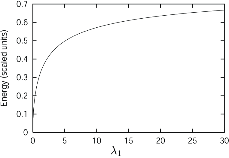
FIG. 4.: Energy per unit area as a function of $\lambda_{1}$ for asymmetric kinks. For symmetric kinks, replace $\lambda_{1}$ by $\lambda_{1}+\lambda_{2}$.

So, for given values of $\lambda_{1}$ and $\lambda_{2}$ obeying Eq. (9) there are both asymmetric and symmetric kink solutions. Which one is energetically favoured and therefore stable? We immediately observe that it depends simply on which of $\lambda_{1}$ or $\lambda_{1}+\lambda_{2}$ is larger, i.e. on the sign of $\lambda_{2}$. The clash of symmetries is energetically favoured if $\lambda_{2}>0$ and energetically disfavoured if $\lambda_{2}<0$.

III Planar wall-junction configuration

A Overview and numerical solution

Our toy model was chosen to produce a vacuum manifold of three disconnected pieces I-III as per Eqs. (6)-(8). (The threefold structure is motivated by $E_{6}$, see Section IV below.) Each one-dimensional kink configuration, however, makes use of only two out of the three possibilities. In the context of model building, even if we are only playing with toys at this stage, it seems more natural to use all three pieces equally. Perhaps more importantly, clash-induced symmetry breaking will be enhanced through the presence of all three vacuum types.

To that end, we search for a domain wall junction configuration as depicted in Fig. 5. Three semi-infinite walls meet at a point, the origin or nexus, at angles of $2\pi/3$, dividing the two-dimensional plane into three sectors labelled I-III. Let $(r,\theta)$ be the usual plane polar coordinates. We impose boundary conditions in the obvious way: for a given $\theta$ in sector I, the configuration is required to tend to a vacuum I state as $r\to\infty$, with corresponding conditions in sectors II and III. Away from the nexus, and close to a wall, we expect the configuration to tend to a one-dimensional kink as a function of the coordinate perpendicular to the wall. Let us call this set-up a “three-star”. To calculate it, one must solve the equations of motion, this time using the two-dimensional Laplacian in place of $d^{2}/dz^{2}$ on the left-hand side of Eq. (19), static and $z$-independent solutions being sought.

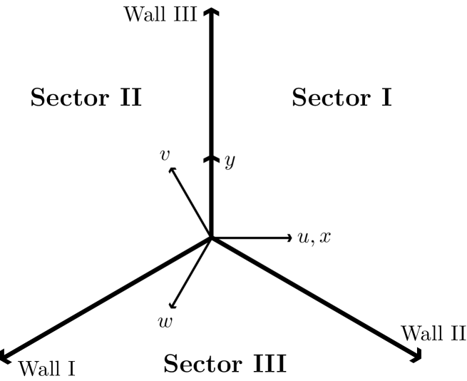
FIG. 5.: The three-star domain wall junction configuration. Each wall makes a $2\pi/3$ angle with the neighbouring walls. In Sector I, a vacuum I state is reached asymptotically; correspondingly in Sectors II and III. The two coordinate systems, $(x,y)$ and $(u,v,w)$, are indicated.

The brane limit is most conveniently written in terms of the Mandelstam-like variables (see Fig. 5),

$$u=x,\quad v=-\frac{1}{2}x+\frac{\sqrt{3}}{2}y,\quad w=-u-v=-\frac{1}{2}x-\frac{\sqrt{3}}{2}y,$$ (36)

as

$$\phi_{1}\to\Theta(u)\Theta(-w),\quad\phi_{2}\to\Theta(v)\Theta(-u),\quad\phi_{3}\to\Theta(w)\Theta(-v).$$ (37)

(It is tempting to “regularise” this configuration by replacing each $\Theta$ with a $(1+\tanh)/2$. We have checked that this suggestive form captures the spirit of the three-star we have produced numerically, but not its detail.)

There are three different types of three-stars: totally symmetric, totally asymmetric, and mixed. The symmetric star has the asymptotic vacuum states being cyclic permutations of [$\langle\Phi_{1}\rangle=(1/\sqrt{2},0,0)^{T}$, $\langle\Phi_{2}\rangle=(0,0,0)^{T}$, $\langle\Phi_{3}\rangle=(0,0,0)^{T}$]. There is no clash of symmetries anywhere for this case: the unbroken symmetry is U(2)${}_{\text{I}}$ everywhere.

The configuration we want is the totally asymmetric star, defined by the vacuum states:

$$\text{Sector I:}\quad\langle\Phi_{1}\rangle=(1/\sqrt{2},0,0)^{T},\quad\langle\Phi_{2}\rangle=(0,0,0)^{T},\quad\langle\Phi_{3}\rangle=(0,0,0)^{T},$$ (38)

$$\text{Sector II:}\quad\langle\Phi_{1}\rangle=(0,0,0)^{T},\quad\langle\Phi_{2}\rangle=(0,1/\sqrt{2},0)^{T},\quad\langle\Phi_{3}\rangle=(0,0,0)^{T},$$ (39)

$$\text{Sector III:}\quad\langle\Phi_{1}\rangle=(0,0,0)^{T},\quad\langle\Phi_{2}\rangle=(0,0,0)^{T},\quad\langle\Phi_{3}\rangle=(0,0,1/\sqrt{2})^{T}.$$ (40)

Ignoring the superfluous U(1)’s, the clash of symmetries has the pattern:

$$H_{\text{I}\cap\text{II}}=\text{U}(2)_{\text{I}}\cap\text{U}(2)_{\text{II}}=\text{U}(1)_{\text{III}}\ \text{along wall III},$$ (41)

$$H_{\text{II}\cap\text{III}}=\text{U}(2)_{\text{II}}\cap\text{U}(2)_{\text{III}}=\text{U}(1)_{\text{I}}\ \text{along wall I},$$ (42)

$$H_{\text{III}\cap\text{I}}=\text{U}(2)_{\text{III}}\cap\text{U}(2)_{\text{I}}=\text{U}(1)_{\text{II}}\ \text{along wall II}.$$ (43)

At the nexus, the symmetry is completely destroyed:

$$H_{\text{I}\cap\text{II}\cap\text{III}}=\text{U}(2)_{\text{I}}\cap\text{U}(2)_{\text{II}}\cap\text{U}(2)_{\text{III}}=\{1\}.$$ (44)

The totally asymmetric star is energetically favoured over the mixed and symmetric stars for the same region of parameter space in which the asymmetric kink is favoured over the symmetric one. We place our toy $3+1$-dimensional universe at the nexus.

Figures 6, 7 and 8 show the $\phi_{1}$, $\phi_{2}$ and $\phi_{3}$ components of the numerically computed asymmetric three-star for the parameter point $\lambda_{1}=4$. Figure 9 displays the energy density of the three-star as a function of $x$ and $y$. We expect that the three-star, defined by the $2\pi/3$ angular separation of the walls, is the lowest energy three-wall junction configuration because it minimises the total length of the domain walls. We have checked this numerically: in our simulations, junctions with unequal angles between the walls relax to the $2\pi/3$ angular configuration we describe.

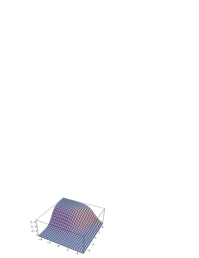
FIG. 6.: The $\phi_{1}$ component of the asymmetric three-star configuration for $\lambda_{1}=4$ as a function of $x$ and $y$.

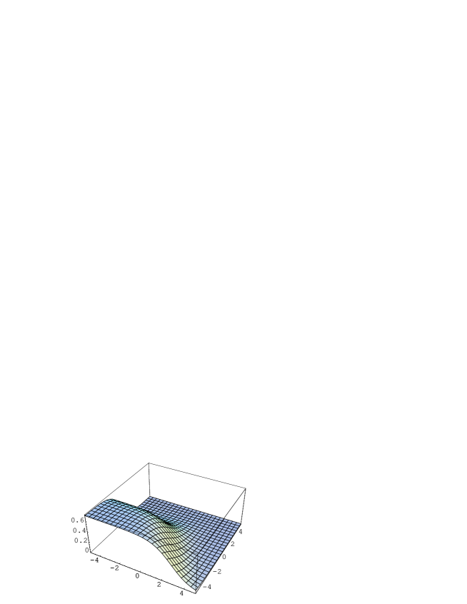
FIG. 7.: The $\phi_{2}$ component of the asymmetric three-star configuration for $\lambda_{1}=4$ as a function of $x$ and $y$.

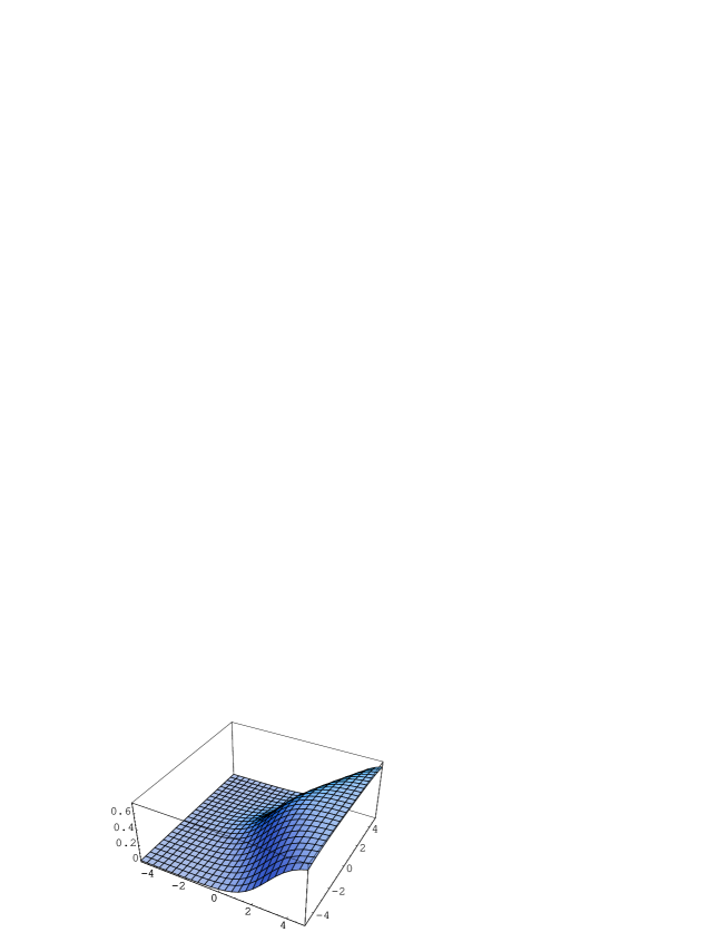
FIG. 8.: The $\phi_{3}$ component of the asymmetric three-star configuration for $\lambda_{1}=4$ as a function of $x$ and $y$.

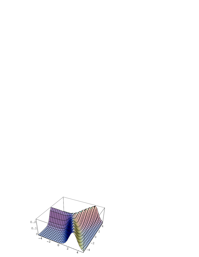
FIG. 9.: The energy density of the asymmetric three-star configuration for $\lambda_{1}=4$ as a function of $x$ and $y$.

B Partial analytical results

We now present some analytical results for two different asymptotic regimes: off-wall and near-wall, both at large $r$.

Note first, though, that the threefold symmetry of the star implies that if

$$\phi_{1}(r,\theta)=\psi(r,\theta)$$ (45)

then

$$\phi_{2}(r,\theta)=\psi(r,\theta-\frac{2\pi}{3}),\qquad\phi_{3}(r,\theta)=\psi(r,\theta+\frac{2\pi}{3}).$$ (46)

Also, the function $\phi_{1}$ must be symmetric under the reflection $v\to-v$, $\phi_{2}$ under $w\to-w$, and $\phi_{3}$ under $u\to-u$. This is because a sector I vacuum preserves the $\Phi_{2}\leftrightarrow\Phi_{3}$ discrete symmetry, and so on.

1 Large r, off-wall behaviour

At large $r$, put

$$\phi_{1}(r,\theta)=f(\theta)+\epsilon(r,\theta),$$ (47)

where

$$f(\theta)=\left\{\begin{array}[]{cc}1/\sqrt{2}&\quad\text{in sector I}\\ 0&\quad\text{elsewhere,}\end{array}\right.$$ (48)

and $\epsilon(r,\theta)\ll 1$. Equation (46) is then used to determine $\phi_{2,3}(r,\theta)$. The perturbative requirement that the function $\epsilon(r,\theta)$ be small is met off-wall and at large $r$.

Substituting Eq. (47) into the Euler-Lagrange equations, and equating like powers of $\epsilon$ one obtains to zeroth order

$$\frac{1}{r^{2}}\frac{d^{2}f}{d\theta^{2}}(\theta)=f(\theta)\left\{-1+2f(\theta)^{2}+(2+\lambda_{1})\left[f(\theta-\frac{2\pi}{3})^{2}+f(\theta+\frac{2\pi}{3})^{2}\right]\right\},$$ (49)

and to first order

$$\left[\frac{\partial^{2}}{\partial r^{2}}+\frac{1}{r}\frac{\partial}{\partial r}+\frac{1}{r^{2}}\frac{\partial^{2}}{\partial\theta^{2}}\right]\epsilon(r,\theta) = \left\{-1+6f(\theta)^{2}+(2+\lambda_{1})\left[f(\theta-\frac{2\pi}{3})^{2}+f(\theta+\frac{2\pi}{3})^{2}\right]\right\}\epsilon(r,\theta)$$ (50)

$$+ 2(2+\lambda_{1})f(\theta)\left[f(\theta-\frac{2\pi}{3})\epsilon(r,\theta-\frac{2\pi}{3})+f(\theta+\frac{2\pi}{3})\epsilon(r,\theta+\frac{2\pi}{3})\right].$$ (51)

The zeroth order equation is satisfied by the $f$ defined in Eq. (48).

The right-hand side of Eq. (51) must be treated on a sector by sector basis. It gives rise to

$$\left[\frac{\partial^{2}}{\partial r^{2}}+\frac{1}{r}\frac{\partial}{\partial r}+\frac{1}{r^{2}}\frac{\partial^{2}}{\partial\theta^{2}}\right]\epsilon(r,\theta)=\left\{\begin{array}[]{cc}2\epsilon(r,\theta)&\quad\text{for}\ \theta\ \text{in sector I},\\ \frac{\lambda_{1}}{2}\epsilon(r,\theta)&\quad\text{elsewhere,}\end{array}\right.$$ (52)

remembering that we must stay off-wall.

To solve Eq. (52), we look for separated variable solutions,

$$\epsilon(r,\theta)=R(r)T(\theta).$$ (53)

Substituting in Eq. (52) produces

$$T^{\prime\prime}(\theta) = -n^{2}T(\theta),$$ (54)

$$R^{\prime\prime}(r)+\frac{1}{r}R^{\prime}(r) = \left(k^{2}+\frac{n^{2}}{r^{2}}\right)R(r),$$ (55)

where $k^{2}=2$ for $\theta$ in sector I and $k^{2}=\lambda_{1}/2$ otherwise, and we define $k$ to be positive. The separation constant is $n^{2}$, and we require it to be positive. Equation (54) is solved by $T(\theta)=T_{n}(\theta)\propto\cos(n\theta+\delta)$, where periodicity in $\theta$ requires $n$ to be an integer, and $\delta$ is determined by requiring symmetry under $v\to-v$ (if $\theta=0$ is the $v=0$ line bisecting sector I, then $\delta=0$).

The radial equation (55) has general solution

$$R(r)=c_{1}I_{n}(kr)+c_{2}K_{n}(kr)$$ (56)

where $c_{{1,2}}$ are constants and $I_{n}$ and $K_{n}$ are modified Bessel functions. The boundary conditions require us to choose

$$R(r)\propto R_{n}(r)\equiv K_{n}(kr),$$ (57)

which, for all $n$, has asymptotic behaviour

$$R_{n}(r)\sim\frac{e^{-kr}}{\sqrt{kr}}.$$ (58)

Writing the general solution to Eq. (52) as a sum over $n$ of $R_{n}(r)T_{n}(\theta)$ with undetermined coefficients, we find that

$$\epsilon(r,\theta)\sim\frac{e^{-kr}}{\sqrt{kr}}F(\theta),$$ (59)

where $F$ is an undetermined angular function. The nature of $F$ may well be different in sectors II and III from sector I, just as the inverse decay length $k$ takes different values if $\lambda_{1}\neq 4$. Notice that $\lambda_{1}=4$ is the same special point that produces hyperbolic tangent kinks. We saw earlier that these kinks have the special property $\phi_{1,2}(z)+\phi_{1,2}(-z)=1/\sqrt{2}$ (taking the I $\leftrightarrow$ II case). The equality of the $k$’s on both sides of the wall is a similar special property for the star configuration.

2 Large $r$, near-wall behaviour

We will now explore near-wall behaviour far from the nexus, using wall II as our example. To begin with, the relevant coordinates are $\rho$, the radial distance directly along the wall, and $w$, perpendicular to the wall.

We again use a perturbative approach, writing

$$\phi_{1}(\rho,w) = g(w)+\delta(\rho,w),$$ (60)

$$\phi_{2} \simeq 0,$$ (61)

$$\phi_{3}(\rho,w) = g(-w)+\delta(\rho,-w),$$ (62)

where $\delta$ is small. The $w$-parity relationship between $\phi_{1}$ and $\phi_{3}$ is dictated by the threefold and reflection symmetries of the configuration. Although the $\phi_{2}$ field is of order $\delta(\rho,w)$ along wall II at large $\rho$, it enters quadratically into the Euler-Lagrange equations for $\phi_{1,3}$ so can be set to zero a priori.

Note that the regime we explore here is physically separated from the off-wall regime probed above, even though both lie far from the nexus. If we set $w$ to some finite value and take $\rho\to\infty$, then the angular distance from the wall goes to zero: $\Delta\theta\sim w/\rho\to 0$. By contrast, the off-wall region requires finite $\Delta\theta$.

Substitution of Eqs. (60)-(62) into the Euler-Lagrange equations yields the zeroth order result

$$g^{\prime\prime}(w)=g(w)\left[-1+2g(w)^{2}+(2+\lambda_{1})g(-w)^{2}\right].$$ (63)

By symmetry, a similar equation with $w\to-w$ also holds. Defining

$$S_{0}(w)=g(w)+g(-w),\qquad A_{0}(w)=g(w)-g(-w),$$ (64)

we recover Eqs. (21) and (22). This shows very clearly that the perpendicular near-wall behaviour far from the origin is exactly the appropriate one-dimensional kink.

The first order analysis depends on the function $g$. To proceed analytically, we restrict the following to the special $\lambda_{1}=4$ case, so that $g(w)=[1+\tanh(w/\sqrt{2})]/2\sqrt{2}$. Setting

$$S\equiv\phi_{1}+\phi_{3}=S_{0}(w)+\delta\!S,\quad A\equiv\phi_{1}-\phi_{3}=A_{0}(w)+\delta\!A,$$ (65)

substituting in the Euler-Lagrange equations, and equating terms to first order in $\delta\!S$ and $\delta\!A$ we obtain:

$$\nabla^{2}(\delta\!S) = \delta\!S(-1+6S_{0}^{2})=2\delta\!S,$$ (66)

$$\nabla^{2}(\delta\!A) = \delta\!A(-1+6A_{0}^{2}),$$ (67)

where we have also used $S_{0}(w)=1/\sqrt{2}$.

We now switch to polar coordinates $(r,\eta)$ where $\tan\eta=w/\rho$ and $r^{2}=\rho^{2}+w^{2}$. Searching for separated variable solutions in these coordinates, we set

$$\delta\!S(r,\eta)=P(r)[W(\eta)+W(-\eta)],\quad\delta\!A(r,\eta)=P(r)[W(\eta)-W(-\eta)].$$ (68)

Substitution in Eq. (66) then immediately yields

$$P^{\prime\prime}(r)+\frac{1}{r}P^{\prime}(r)=(2+\frac{n^{2}}{r^{2}})P(r),$$ (69)

where $n^{2}>0$ is the separation constant. We conclude that

$$P(r)\sim\frac{e^{-\sqrt{2}r}}{\sqrt{\sqrt{2}r}},\quad\forall n$$ (70)

which matches exactly the asymptotic radial behaviour, Eq. (58), found earlier in the off-wall regime.

Consider now Eq. (67). Using Eq. (69) and the known function $g$, defining $\Delta(\eta)=W(\eta)-W(-\eta)$, we obtain

$$\frac{\Delta^{\prime\prime}(\eta)}{r^{2}\Delta(\eta)}=-3-\frac{n^{2}}{r^{2}}+3\tanh^{2}\left(\frac{r\sin\eta}{\sqrt{2}}\right).$$ (71)

For large $r$, the term depending on the separation constant $n^{2}$ is suppressed and can be omitted. For small $\eta$, we can change variables to $w=r\eta$ to get

$$\frac{\Delta^{\prime\prime}(w)}{\Delta(w)}\approx-3+3\tanh^{2}\frac{w}{\sqrt{2}}.$$ (72)

The solution with the correct antisymmetry in $w$ is then

$$\Delta(w)\propto\left[3\tanh\frac{w}{\sqrt{2}}+\frac{w}{\sqrt{2}}\left(1-3\tanh^{2}\frac{w}{\sqrt{2}}\right)\right].$$ (73)

The collection of results above demonstrates that one can make some progress in understanding the three-star configuration analytically, even though an exact analytic solution is at present lacking.

IV Discussion

Our toy model was chosen not only to be mathematically simple, but also because it can serve as a prototype for a more realistic theory motivated by E₆. While it is beyond the scope of this paper to explore this connection in detail, we would like to comment and speculate on possible future directions.

The most direct connection is with the maximal SU(3)³ subgroup of E₆, augmented by a discrete Z₃ symmetry that rotates the SU(3) factors. The complex, anomaly-free representation

$$(3,\overline{3},1)\oplus(1,3,\overline{3})\oplus(\overline{3},1,3),$$ (74)

which arises from the decomposition of the $27$ of E₆, naturally generalises the three triplet Higgs boson content of the toy model. As is well known, one generation of quarks and leptons can be placed in a similar representation. It would be interesting to apply the clash of symmetries idea in this context, to see what symmetry breaking patterns can be produced.

In the future pursuit of serious brane model-building, there is no reason to restrict Higgs potentials to quartic form. If, for instance, we have a three-star configuration in mind, then the underlying spacetime is at least $5+1$ dimensional, where renormalisability requires at most cubic potentials (which are necessarily unbounded from below and thus presumably unacceptable). The question of renormalisation should sensibly be deferred until such time as a connection with a proper theory of quantum gravity can be made. We recognise that many string-theoretic brane and brane junction scenarios have already been proposed [9].

If the full E₆ is considered rather than just the SU(3)³ subgroup, then an important issue is domain wall stability. The Z₃ symmetry of the reduced theory, useful for wall stability, is then presumably embedded within the continuous E₆ symmetry. According to the general understanding of defect formation, the breakdown of E₆ to, first, SU(3)³ $\otimes$ Z₃, and then to some smaller subgroup, will imply the existence of unstable vortex-wall hybrid structures rather than topologically stable walls. While it may be possible for the instability timescale to be very long, a bulk scalar field in the $27$ of E₆ offers another natural possibility. Recognising that singlets arise in the products $27\otimes\overline{27}$ and $27\otimes 27\otimes 27$, we see that a general Higgs potential will respect a $Z_{3}$ phase symmetry that may not be contained within E₆.

The number “3” plays a prominent role in the group theory of E₆: there are three SU(3) factors in the maximal subgroup under discussion, and there are also three ways to embed electric charge $Q$ within the group. The latter fact has been remarked on before [10], but perhaps it has not received the attention it deserves. From the perspective of the subgroup chain E₆ $\to$ SO(10)$\otimes$U(1)^′′ $\to$ SU(5)$\otimes$U(1)^′$\otimes$U(1)^′′, the three electric charge assignments correspond to the standard case where $Q$ lies within SU(5), the flipped SU(5) case where U(1)^′ is also involved, and the flipped SO(10) case where U(1)^′′ enters the definition of $Q$. Now, there is another long-standing mystery pertaining to the number three: the apparently superfluous replication of quark-lepton families. The lack of a compelling explanation despite years of thought suggests that new approaches should be seriously considered. We speculate that the three $Q$ embeddings, the three-star configuration derived from the triply degenerate vacuum structure, and threefold quark/lepton family replication may be connected.

V Conclusion

Using a model field theory comprising three U(3) Higgs triplets interacting through a permutation symmetric quartic potential, we have shown that domain wall and wall-junction solutions exist displaying the “clash of symmetries”. This symmetry breaking mechanism goes beyond standard spontaneous breaking by exploiting different embeddings of isomorphic subgroups in the parent group. Our example used the $I$-, $U$- and $V$-spin U(2) subgroups of U(3). We found topologically stable domain wall solutions which asymptote to vacuum states corresponding to differently embedded unbroken U(2) subgroups on opposite sides of the wall. Non-asymptotically, the symmetry is further broken to the intersection of the asymptotically unbroken subgroups. This phenomenon has been previosuly displayed in a different model and with different motivations in Ref. [6]. We propose that such a kink-like configuration in the thin-wall or brane limit may exist in a large extra dimension, with our universe identified with the brane. In that case, some of the symmetry breaking in our universe may be due to the clash of symmetries. Increasing the number of spatial dimensions (notionally) to five, we numerically constructed a wall-junction three-star configuration that exploits the clash phenomenon to the full, with the joint or nexus identified with our (toy) universe. Future work is motivated on several fronts: a possible connection with E₆, a possible connection between the three-star and threefold family replication, and degree of freedom localisation to the brane.

A Justification of the kink ansatz

In this appendix, we justify the asymmetric kink ansatz used in Section II C. We consider the case $\lambda_{2}>0$ and show that a globally stable kink must fit this ansatz, Eq. (18). (Analogous arguments show that the symmetric kink is globally stable for $\lambda_{2}<0$.)

1 The two-triplet model

We begin by considering a simpler model with just two triplets and an exchange discrete symmetry. The Higgs potential is obtained from Eq. (4) by taking $\Phi_{3}=0$.

Consider a general trial solution of the form

$$\Phi_{i}(z)=\left(\phi_{i,1}(z),\phi_{i,2}(z),\phi_{i,3}(z)\right)^{T},$$ (A1)

with $i=1,2,3$, which satisfies the asymmetric boundary conditions:

$$\Phi_{1}(-\infty)=\left(\frac{1}{\sqrt{2}},0,0\right)^{T},\qquad\Phi_{2}(-\infty)=\left(0,0,0\right)^{T},$$ (A2)

$$\Phi_{1}(+\infty)=\left(0,0,0\right)^{T},\qquad\Phi_{2}(+\infty)=\left(0,\frac{1}{\sqrt{2}},0\right)^{T}.$$ (A3)

Define

$$\theta_{i}=\sqrt{\phi_{i,1}^{*}\phi_{i,1}+\phi_{i,2}^{*}\phi_{i,2}+\phi_{i,3}^{*}\phi_{i,3}},$$ (A4)

and consider a second trial solution of the form

$$\Theta_{1}(z) = \left(\theta_{1}(z),0,0\right)^{T},$$ (A5)

$$\Theta_{2}(z) = \left(0,\theta_{2}(z),0\right)^{T}.$$ (A6)

We will show that the configuration of Eq. (A6) has energy less than or equal to the energy of the initial trial solution of Eq. (A1). It is clear that this configuration satisfies the boundary conditions.

Consider first the potential energy density $V\left[\Phi_{1},\Phi_{2}\right]$. Clearly $\Phi_{1}^{\dagger}\Phi_{1}=\Theta_{1}^{\dagger}\Theta_{1}$ and $\Phi_{2}^{\dagger}\Phi_{2}=\Theta_{2}^{\dagger}\Theta_{2}$, so we need only consider the term in the potential dependent on $\lambda_{2}$. But if $\lambda_{2}>0$, then this term is positive for $\Phi_{1,2}$ of the form of Eq. (A1) but zero for the configuration of Eq. (A6). Thus $V\left[\Theta_{1},\Theta_{2}\right]\leq V\left[\Phi_{1},\Phi_{2}\right]$.

We now turn to the kinetic energy density $T\left[\Theta_{1},\Theta_{2}\right]$:

$$\sum_{i}{\Theta_{i}^{\prime}}^{\dagger}\Theta_{i}^{\prime} = \sum_{i}\left(\theta_{i}^{\prime}\right)^{2}$$ (A7)

$$= \sum_{i}\frac{1}{4\theta_{i}^{2}}\left(\phi_{i,1}^{*}\phi_{i,1}^{\prime}+\phi_{i,2}^{*}\phi_{i,2}^{\prime}+\phi_{i,3}^{*}\phi_{i,3}^{\prime}+\ \mathrm{c.\ c.}\right)^{2}$$ (A8)

$$\leq \sum_{i}\frac{1}{\theta_{i}^{2}}\left(\left|\phi_{i,1}\right|\left|\phi_{i,1}^{\prime}\right|+\left|\phi_{i,2}\right|\left|\phi_{i,2}^{\prime}\right|+\left|\phi_{i,3}\right|\left|\phi_{i,3}^{\prime}\right|\right)^{2}$$ (A9)

$$\leq \frac{\left(\left|\phi_{i,1}\right|^{2}+\left|\phi_{i,2}\right|^{2}+\left|\phi_{i,3}\right|^{2}\right)}{\theta_{i}^{2}}\,\left(\left|\phi_{i,1}^{\prime}\right|^{2}+\left|\phi_{i,2}^{\prime}\right|^{2}+\left|\phi_{i,3}^{\prime}\right|^{2}\right)$$ (A10)

$$= \sum_{i}{\Phi_{i}^{\prime}}^{\dagger}\Phi_{i}^{\prime},$$ (A11)

by the Cauchy-Schwarz inequality. So $T\left[\Theta_{1},\Theta_{2}\right]\leq T\left[\Phi_{1},\Phi_{2}\right]$, also.

a The three-triplet Model

We now add the third triplet to the model. Staying with $\lambda_{2}>0$ and applying the arguments of the previous section, it suffices to consider a trial solution of the form

$$\Phi_{1}(z) = \left[\phi_{1}(z),0,0\right]^{T},$$ (A12)

$$\Phi_{2}(z) = \left[0,\phi_{2}(z),0\right]^{T},$$ (A13)

$$\Phi_{3}(z) = \left[0,0,\phi_{3}(z)\right]^{T},$$ (A14)

with $\phi_{i}$ real. Note that the boundary conditions on $\phi_{3}$ require it to vanish asymptotically. We now establish that this trial solution has energy greater than or equal to the alternative trial solution,

$$\Theta_{1}(z) = \left(\sqrt{\left[\phi_{1}(z)\right]^{2}+\left[\phi_{3}(z)\right]^{2}},0,0\right)^{T},$$ (A15)

$$\Theta_{2}(z) = \left(0,\phi_{2}(z),0\right)^{T},$$ (A16)

$$\Theta_{3}(z) = \left(0,0,0\right)^{T}.$$ (A17)

Observe that $\xi(z)\equiv\sqrt{\left[\phi_{1}(z)\right]^{2}+\left[\phi_{3}(z)\right]^{2}}$ obeys the correct boundary conditions. Now, the kinetic energy density due to $\xi$ obeys $(\xi^{\prime})^{2}<(\phi^{\prime}_{1})^{2}+(\phi^{\prime}_{3})^{2}$ by the Cauchy-Schwarz inequality. In the potential energy density function, we need only consider the $\lambda_{1}$ term. For trial solution Eq. (A14) this term is $\lambda_{1}(\phi_{1}^{2}\phi_{2}^{2}+\phi_{2}^{2}\phi_{3}^{2}+\phi_{3}^{2}\phi_{1}^{2})$, while for trial solution Eq. (A17) it is $\lambda_{1}(\xi^{2}\phi_{2}^{2})=\lambda_{1}(\phi_{1}^{2}\phi_{2}^{2}+\phi_{3}^{2}\phi_{2}^{2})$. The latter is obviously smaller than the former.

So globally stable solutions in the two-triplet model are also globally stable in the full three-triplet model.

B Global stability of the $\lambda_{1}=4$ analytic solution

Consider the special parameter point $\lambda_{1}=4$. We prove global stability of the analytic solution, Eqs. (25) and (26), by Bogomolnyi’s method [11]. The energy density $\epsilon\left[\phi_{1},\phi_{2}\right]$ of any solution fitting the ansatz given in Eq. (18) is

$$\epsilon\left[\phi_{1},\phi_{2}\right] = {\phi_{1}^{\prime}}^{2}+{\phi_{2}^{\prime}}^{2}+V\left(\phi_{1},\phi_{2}\right)+\frac{1}{4}$$ (B1)

$$= \left(\phi_{1}^{\prime}+\phi_{1}^{2}+\phi_{2}^{2}-\frac{1}{2}\right)^{2}+\left(\phi_{2}^{\prime}+2\phi_{1}\phi_{2}\right)^{2}+\frac{d}{dz}\left(\phi_{1}-\frac{2}{3}\,\phi_{1}^{3}-2\phi_{2}^{2}\phi_{1}\right).$$ (B2)

The first two terms of this equation are non-negative, so the total kink energy is

$$\int_{-\infty}^{\infty}\epsilon\left[\phi_{1},\phi_{2}\right]dz\geq\int_{-\infty}^{\infty}dz\,\frac{d}{dz}\left({\phi_{1}}-\frac{2}{3}\,\phi_{1}^{3}-2\phi_{2}^{2}\phi_{1}\right)=\frac{\sqrt{2}}{3},$$ (B3)

where we have substituted for the boundary conditions. Since the analytic solution given in the main text, Eq. (33) saturates this lower bound, it is globally stable.

REFERENCES

- [1] E. P. S. Shellard and A. Vilenkin, Cosmic Strings and other topological defects (Cambridge University Press, Cambridge, 1994); R. Rajaraman, Solitons and Instantons (North Holland Pub. Co., Amsterdam, 1982); and references therein.
- [2] Ya. B. Zel’dovich, I. Yu. Kobzarev and L. B. Okun, Zh. Eksp. Teor. Fiz. 67, 3 (1974) [Sov. Phys. JETP 40, 1 (1974)].
- [3] V. A. Rubakov and M. E. Shaposhnikov, Phys. Lett. B125, 136 (1983).
- [4] N. Arkani-Hamed, S. Dimopoulos and G. R. Dvali, Phys. Lett. B429, 263 (1998); L. J. Randall and R. Sundrum, Phys. Rev. Lett. 83, 3370 (1999); 83, 4690 (1999); T. Regge and C. Teitelboim, in Proceedings of the Marcel Grossman Conference (Trieste, 1975); A. Davidson and D. Karasik, Mod. Phys. Lett. A13, 2187 (1998); A. Davidson, Class. Quant. Grav. 16, 653 (1999).
- [5] C. Csaki and Y. Shirman, Phys. Rev. D61, 024008 (1999).
- [6] L. Pogosian and T. Vachaspati, Phys. Rev. D62, 123506 (2000). See also T. Vachaspati, Phys. Rev. D63, 105010 (2001); L. Pogosian and T. Vachaspati, Phys. Rev. D64, 105023 (2001).
- [7] G. Dvali, Z. Tavartkiladze and J. Nanobashvili, Phys. Lett. B352, 214 (1994).
- [8] T. Nihei, Phys. Rev. D62, 124017 (2000); S. M. Carroll, S. Hellerman and M. Trodden, Phys. Rev. D61, 065001 (2000); D62, 044049 (2000).
- [9] See, for example, L. E. Ibáñez, F. Marchesano and R. Rabadán, hep-th/0105155.
- [10] M. Bando and T. Kugo, Prog. Theor. Phys. 101, 1313 (1999); M. Bando, T. Kugo and K. Yoshioka, Prog. Theor. Phys. 104, 211 (2000); G. W. Anderson and T. Blazek, J. Math. Phys. 41, 4808 (2000).
- [11] E. B. Bogomol’nyi, Sov. J. Nucl. Phys., 24, No. 4 (1976), reprinted in C. Rebbi and G. Soliani, Solitons and Particles (World Scientific, Singapore, 1984).