31st January 2002

String Cosmology

Edmund.J. Copeland

Centre for Theoretical Physics, University of Sussex, Falmer, Brighton BN1 9QJ,   U. K.

We present a brief review of recent advances in string cosmology. Starting with the Dilaton-Moduli Cosmology (known also as the Pre Big Bang), we go on to include the effects of axion fields and address the thorny issue of the Graceful Exit in String Cosmology. This is followed by a review of density perturbations arising in string cosmology and we finish with a brief introduction to the impact moving five branes can have on the Dilaton-Moduli cosmological solutions.

PRESENTED AT

COSMO-01
Rovaniemi, Finland,
August 29 – September 4, 2001

1 Introduction

String theory, and its most recent incarnation, that of M-theory, has been accepted by many as the most likely candidate theory to unify the forces of nature as it includes General Relativity in a consistent quantum theory. If it is to play such a pivotal role in particle physics, it should also include in it all of cosmology. It should provide the initial conditions for the Universe, perhaps even explain away the singularity associated with the standard big bang. It should also provide a mechanism for explaining the observed density fluctuations, perhaps by providing the inflaton field or some other mechanism which would lead to inflation. Should the observations survive the test of time, string theory should be able to provide a mechanism to explain the current accelerated expansion of the Universe. In other words, even though it is strictly a theory which can unify gravity with the other forces in the very early Universe, for consistency, as a theory of everything it will have a great deal more to explain. In this article, we will introduce some of the developments that have occurred in string cosmology over the past decade or so, initially basing the discussion on an analyse of the low energy limit of string theory, and then later extending it to include branes arising in Heterotic M-theory.

2 Dilaton-Moduli Cosmology (Pre-Big Bang)

Strings live in 4+d spacetime dimensions, with the extra $d$ dimensions being compactified. For homogeneous, four–dimensional cosmologies, where all fields are uniform on the surfaces of homogeneity, we can consider the compactification of the $(4+d)$–dimensional theory on an isotropic $d$–torus. The radius, or ‘breathing mode’ of the internal space, is then parameterized by a modulus field, $\beta$, and determines the volume of the internal dimensions. We can then assume that the $(4+d)$–dimensional metric is of the form

$$ds^{2}=-dt^{2}+g_{ij}dx^{i}dx^{j}+e^{\sqrt{2/d}\beta}\delta_{ab}dX^{a}dX^{b}$$ (1)

where indices run from $(i,j)=(1,2,3)$ and $(a,b)=(4,\ldots,3+d)$ and $\delta_{ab}$ is the $d$–dimensional Kronecker delta. The modulus field $\beta$ is normalized in such a way that it becomes minimally coupled to gravity in the Einstein frame.

The low energy action that is commonly used as a starting point for string cosmology is the four dimensional effective Neveu-Schwarz- Neveu-Schwarz (NS-NS) action given by:

$$S_{*}=\int d^{4}x\sqrt{|g|}e^{-\varphi}\left[R+\left(\nabla\varphi\right)^{2}-\frac{1}{2}\left(\nabla\beta\right)^{2}-\frac{1}{2}e^{2\varphi}\left(\nabla\sigma\right)^{2}\right]\,,$$ (2)

where $\varphi$ is the effective dilaton in four dimensions, and $\sigma$ is the pseudo–scalar axion field which is dual to the fundamental NS–NS three–form field strength present in string theory, the duality being given by

$$H^{\mu\nu\lambda}=\epsilon^{\mu\nu\lambda\kappa}\,e^{\varphi}\,\nabla_{\kappa}\sigma.$$ (3)

The dimensionally reduced action (2) may be viewed as the prototype action for string cosmology because it contains many of the key features common to more general actions. Cosmological solutions to these actions have been extensively discussed in the literature – for a review see [1]. Some of them play a central role in the pre–big bang inflationary scenario, first proposed by Veneziano [2, 3]. An important point can be seen immediately in (2) where there is a non-trivial coupling of the dilaton to the axion field, a coupling which will play a key role later on when we are investigating the density perturbations arising in this scenario.

All homogeneous and isotropic external four–dimensional spacetimes can be described by the Friedmann-Robertson-Walker (FRW) metric. The general line element in the string frame can be written as

$$ds_{4}^{2}=a^{2}(\eta)\left\{-d\eta^{2}+d\Omega_{\kappa}^{2}\right\}\,,$$ (4)

where $a(\eta)$ is the scale factor of the universe, $\eta$ is the conformal time and $d\Omega_{\kappa}^{2}$ is the line element on a 3-space with constant curvature $\kappa$:

$$d\Omega^{2}_{\kappa}=d\psi^{2}+\left(\frac{\sin\sqrt{\kappa}\psi}{\sqrt{\kappa}}\right)^{2}\left(d\theta^{2}+\sin^{2}\theta d\varphi^{2}\right)$$ (5)

To be compatible with a homogeneous and isotropic metric, all fields, including the pseudo–scalar axion field, must be spatially homogeneous.

The models with vanishing form fields, but time-dependent dilaton and moduli fields, are known as dilaton-moduli-vacuum solutions. In the Einstein–frame, these solutions may be interpreted as FRW cosmologies for a stiff perfect fluid, where the speed of sound equals the speed of light. The dilaton and moduli fields behave collectively as a massless, minimally coupled scalar field, and the scale factor in the Einstein frame is given by

$$\tilde{a}=\tilde{a}_{*}\sqrt{\frac{\tau}{1+\kappa\tau^{2}}}$$ (6)

where $\tilde{a}\equiv e^{-\varphi/2}a$, $\tilde{a}_{*}$ is a constant and we have defined a new time variable:

$$\tau\equiv\left\{\begin{array}[]{ll}\kappa^{-1/2}|\tan(\kappa^{1/2}\eta)|&{\rm for}\ \kappa>0\\ |\eta|&{\rm for}\ \kappa=0\\ |\kappa|^{-1/2}|\tanh(|\kappa|^{1/2}\eta)|&{\rm for}\ \kappa<0\end{array}\right.\ .$$ (7)

The time coordinate $\tau$ diverges at both early and late times in models which have $\kappa\geq 0$, but $\tau\to|\kappa|^{-1/2}$ in negatively curved models. There is a curvature singularity at $\eta=0$ with $\tilde{a}=0$ and the model expands away from it for $\eta>0$ or collapses towards it for $\eta<0$. The expanding, closed models recollapse at $\eta=\pm\pi/2$ and there are no bouncing solutions in this frame.

The corresponding string frame scale factor, dilaton and modulus fields are given by the ‘rolling radii’ solutions [4]

$$a = a_{*}\sqrt{{\tau^{1+\sqrt{3}\cos\xi_{*}}\over 1+\kappa\tau^{2}}}\,,$$ (8)

$$e^{\varphi} = e^{\varphi_{*}}\tau^{\sqrt{3}\cos\xi_{*}}\,,$$ (9)

$$e^{\beta} = e^{\beta_{*}}\tau^{\sqrt{3}\sin\xi_{*}}\,$$ (10)

The integration constant $\xi_{*}$ determines the rate of change of the effective dilaton relative to the volume of the internal dimensions. Figures 1 and 2 show the dilaton-vacuum solutions in flat FRW models when stable compactification has occurred, so that the volume of the internal space is fixed, with $\xi_{*}\ {\rm mod}\ \pi=0$.

Figure 1: String frame scale factor, $a$, as a function of conformal time, $\eta$, for flat $\kappa=0$ FRW cosmology in dilaton-vacuum solution in Eq. (8) with $\xi_{*}=0$ (dashed-line), $\xi_{*}=\pi$ (dotted line) and dilaton-axion solution in Eq. (13) with $r=\sqrt{3}$ (solid line). The $(+)$ and $(-)$ branches are defined in the text.

Figure 2: Dilaton, $e^{\varphi}$, as a function of conformal time, $\eta$, for flat $\kappa=0$ FRW cosmology in dilaton-vacuum solution in Eq. (9) with $\xi_{*}=0$ (dashed-line), $\xi_{*}=\pi$ (dotted line) and dilaton-axion solution in Eq. (12) with $r=\sqrt{3}$ (solid line).

The solutions just presented have a scale factor duality which when applied simultaneously with time reversal implies that the Hubble expansion parameter $H\equiv d(\ln a)/dt$ remains invariant, $H(-t)\to H(t)$, whilst its first derivative changes sign, $\dot{H}(-t)\to-\dot{H}(t)$. A decelerating, post–big bang solution – characterized by $\dot{a}>0$, $\ddot{a}<0$ and $\dot{H}<0$ – is mapped onto a pre–big bang phase of inflationary expansion, since $\ddot{a}/a=\dot{H}+H^{2}>0$. The Hubble radius $H^{-1}$ decreases with increasing time and the expansion is therefore super-inflationary. Thus, the pre-big bang cosmology ($\kappa=0$ case in Eqns. (8–10)) is one that has a period of super-inflation driven simply by the kinetic energy of the dilaton and moduli fields [2, 3]. This is related by duality to the usual FRW post–big bang phase. The two branches are separated by a curvature singularity, however, and it is not clear how the transition between the pre– and post–big bang phases might proceed. This will be the focus of attention in section five.

The solution for a flat ($\kappa=0$) FRW universe corresponds to the well–known monotonic power-law, or ‘rolling radii’, solutions. For $\cos\xi_{*}<-1/\sqrt{3}$ there is accelerated expansion, i.e., inflation, in the string frame for $\eta<0$ and $e^{\varphi}\to 0$ as $t\to-\infty$, corresponding to the weak coupling regime. The expansion is an example of ‘pole–law’ inflation [5, 6].

The solutions have semi-infinite proper lifetimes. Those starting from a singularity at $t=0$ for $t\geq 0$ are denoted as the (–) branch in Ref. [7], while those which approach a singularity at $t=0$ for $t\leq 0$ are referred to as the $(+)$ branch (see figures 1–2). These $(+/-)$ branches do not refer to the choice of sign for $\cos\xi_{*}$. On either the $(+)$ or $(-)$ branches of the dilaton-moduli-vacuum cosmologies we have a one-parameter family of solutions corresponding to the choice of $\xi_{*}$, which determines whether $e^{\varphi}$ goes to zero or infinity as $t\to 0$. These solutions become singular as the conformally invariant time parameter $\eta\equiv\int dt/a(t)\to 0$ and there is no way of naively connecting the two branches based simply on these solutions [7].

In the Einstein frame, where the dilaton field is minimally coupled to gravity, the scale factor given in Eq. (6), becomes

$$\tilde{a}=\tilde{a}_{*}\left|\eta\right|^{1/2}$$ (11)

As $\eta\to 0$ on the (+) branch, the universe is collapsing with $\tilde{a}\to 0$, and the comoving Hubble length $|d(\ln\tilde{a})/d\eta|^{-1}=2|\eta|$ is decreasing with time. Thus, in both frames there is inflation taking place in the sense that a given comoving scale, which starts arbitrarily far within the Hubble radius in either conformal frame as $\eta\to-\infty$, inevitably becomes larger than the Hubble radius in that frame as $\eta\to 0$. The significance of this is that it means that perturbations can be produced in the dilaton, graviton and other matter fields on scales much larger than the present Hubble radius from quantum fluctuations in flat spacetime at earlier times – this is a vital property of any inflationary scenario.

For completeness, it is worth mentioning that these solutions can be extended to include a time-dependent axion field, $\sigma(t)$, by exploiting the ${\rm SL}(2,R)$ S-duality invariance of the four–dimensional, NS-NS action [4]. We now turn our attention to this fascinating case.

3 Dilaton-Moduli-Axion Cosmologies

The cosmologies containing a non–trivial axion field can be generated immediately due to the global ${\rm SL}(2,R)$ symmetry of the action (2). The resultant solutions are [4]:

$$e^{\varphi} = {e^{\varphi_{*}}\over 2}\left\{\left({\tau\over\tau_{*}}\right)^{-r}+\left({\tau\over\tau_{*}}\right)^{r}\right\}\,,$$ (12)

$$a^{2} = \frac{a_{*}^{2}}{2(1+\kappa\tau^{2})}\left\{\left({\tau\over\tau_{*}}\right)^{1-r}+\left({\tau\over\tau_{*}}\right)^{1+r}\right\}\,,$$ (13)

$$e^{\beta} = e^{\beta_{*}}\tau^{s}\,,$$ (14)

$$\sigma = \sigma_{*}\pm e^{-\varphi_{*}}\left\{(\tau/\tau_{*})^{-r}-(\tau/\tau_{*})^{r}\over(\tau/\tau_{*})^{-r}+(\tau/\tau_{*})^{r}\right\}\,,$$ (15)

where the exponents are related via

$$r^{2}+s^{2}=3\ ,$$ (16)

and without loss of generality we may take $r\geq 0$.

In all cases, the dynamics of the axion field places a lower bound on the value of the dilaton field, $\varphi\geq\varphi_{*}$. In so doing, the axion smoothly interpolates between two dilaton–moduli–vacuum solutions, where its dynamical influence asymptotically becomes negligible. The effects of time–dependent axion solutions for the scale-factor and dilaton are plotted in Figure2 1 and 2 for the flat FRW model when the modulus field is trivial $(s=0)$. When the internal space is static, it is seen that the string frame scale factors exhibit a bounce. However we still have a curvature singularity in the Einstein frame as $\tau\to 0$. The actual time-dependent axion solutions is shown in Figure 3.

Figure 3: Axion, $\sigma$, as a function of conformal time, $\eta$, for flat $\kappa=0$ FRW cosmology in dilaton-axion solution in Eq. (15) with $r=\sqrt{3}$ (solid line).

The spatially flat solutions reduce to the power law, dilaton–moduli–vacuum solution given in Eqs. (8–10) at early and late times. When $\eta\to\pm\infty$ the solution approaches the vacuum solution with $\sqrt{3}\cos\xi_{*}=+r$, while as $\eta\to 0$ the solution approaches the $\sqrt{3}\cos\xi_{*}=-r$ solution. Thus, the axion solution interpolates between two vacuum solutions related by an S-duality transformation $\varphi\to-\varphi$. When the internal space is static the scale factor in the string frame is of the form $a\propto t^{1/\sqrt{3}}$ as $\eta\to\pm\infty$, while as $\eta\to 0$ the solution becomes $a\propto t^{-1/\sqrt{3}}$. These two vacuum solutions are thus related by a scale factor duality that inverts the spatial volume of the universe. This asymptotic approach to dilaton–moduli–vacuum solutions at early and late times will lead to a particularly simple form for the semi-classical perturbation spectra that is independent of the intermediate evolution. However, there is a down side to these solutions from the standpoint of pre big bang cosmologies. As $\eta\to\pm\infty$ and as $\eta\to 0$ the solution approaches the strong coupling regime where $e^{\varphi}\to\infty$. Thus there is no weak coupling limit, the axion interpolates between two strong coupling vacuum solutions. We will shortly see how a similar affect arises when we include a moving brane in the dilaton-moduli picture, as it too mimics the behaviour of a non-minimally coupled axion field.

The overall dynamical effect of the axion field is negligible except near $\tau\approx\tau_{*}$, when it leads to a bounce in the dilaton field. Within the context of M–theory cosmology, the radius of the eleventh dimension is related to the dilaton by $r_{11}\propto e^{\varphi/3}$ when the modulus field is fixed. This bound on the dilaton may therefore be reinterpreted as a lower bound on the size of the eleventh dimension.

4 Fine tuning issues

The question over the viability of the initial conditions required in the pre Big Bang scenario has been a cause for many an argument both in print and in person. Since both $\dot{H}$ and $\dot{\varphi}$ are positive in the pre–big bang phase, the initial values for these parameters must be very small. This raises a number of important issues concerning fine–tuning in the pre–big bang scenario [8, 9, 10, 11, 12, 13, 14]. There needs to be enough inflation in a homogeneous patch in order to solve the horizon and flatness problems which means that the dilaton driven inflation must survive for a sufficiently long period of time. This is not as trivial as it may appear, however, since the period of inflation is limited by a number of factors.

The fundamental postulate of the scenario is that the initial data for inflation lies well within the perturbative regime of string theory, where the curvature and coupling are very small [3]. Inflation then proceeds for sufficiently homogeneous initial conditions [12, 13], where time derivatives are dominant with respect to spatial gradients, and the universe evolves into a high curvature and strongly–coupled regime. Thus, the pre–big bang initial state should correspond to a cold, empty and flat vacuum state. Initial the universe would have been huge relative to the quantum scale and hence should have been well described by classical solutions to the string effective action. This should be compared to the initial state which describes the standard hot big bang, namely a dense, hot, and highly curved region of spacetime. This is quite a contrast and a primary goal of pre–big bang cosmology must be to develop a mechanism for smoothly connecting these two regions, since we believe that the standard big bang model provides a very good representation of the current evolution of the universe.

Our present observable universe appears very nearly homogeneous on sufficiently large scales. In the standard, hot big bang model, it corresponded to a region at the Planck time that was $10^{30}$ times larger than the horizon size, $l_{\rm Pl}$. This may be viewed as an initial condition in the big bang model or as a final condition for inflation. It implies that the comoving Hubble radius, $1/(aH)$, must decrease during inflation by a factor of at least $10^{30}$ if the horizon problem is to be solved. For a power law expansion, this implies that

$$\left|\frac{\eta_{f}}{\eta_{i}}\right|\leq 10^{-30}$$ (17)

where subscripts $i$ and $f$ denote values at the onset and end of inflation, respectively.

In the pre–big bang scenario, Eq. (9) implies that the dilaton grows as $e^{\varphi}\propto|\eta|^{-\sqrt{3}}$, and since at the start of the post–big bang epoch, the string coupling, $g_{s}=e^{\varphi/2}$, should be of order unity, the bound (17) implies that the initial value of the string coupling is strongly constrained, $g_{s,i}\leq 10^{-26}$. Turner and Weinberg interpret this constraint as a severe fine–tuning problem in the scenario, because inflation in the string frame can be delayed by the effects of spatial curvature [8]. It was shown by Clancy, Lidsey and Tavakol that the bounds are further tightened when spatial anisotropy is introduced, actually preventing pre–big bang inflation from occurring [9]. Moreover, as we have seen the dynamics of the NS–NS axion field also places a lower bound on the allowed range of values that the string coupling may take [4]. In the standard inflationary scenario, where the expansion is quasi–exponential, the Hubble radius is approximately constant and $a\propto(-\eta)^{-1}$. Thus, the homogeneous region grows by a factor of $|\eta_{i}/\eta_{f}|$ as inflation proceeds. During a pre–big bang epoch, however, $a\propto(-\eta)^{-1/1+\sqrt{3}}$ and the increase in the size of a homogeneous region is reduced by a factor of at least $10^{30\sqrt{3}/(1+\sqrt{3})}\approx 10^{19}$ relative to that of the standard inflation scenario. This implies that the initial size of the homogeneous region should exceed $10^{19}$ in string units if pre–big bang inflation is to be successful in solving the problems of the big bang model [2, 10]. The occurrence of such a large number was cited by Kaloper, Linde and Bousso as a serious problem of the pre–big bang scenario, because it implies that the universe must already have been large and smooth by the time inflation began [10].

On the other hand, Gasperini has emphasized that the initial homogeneous region of the pre–big bang universe is not larger than the horizon even though it is large relative to the string/Planck scale [15]. The question that then arises when discussing the naturalness, or otherwise, of the above initial conditions is what is the basic unit of length that should be employed. At present, this question has not been addressed in detail.

Veneziano and collaborators conjectured that pre–big bang inflation generically evolves out of an initial state that approaches the Milne universe in the semi–infinite past, $t\rightarrow-\infty$ [12, 13]. The Milne universe may be mapped onto the future (or past) light cone of the origin of Minkowski spacetime and therefore corresponds to a non–standard representation of the string perturbative vacuum. The proposal was that the Milne background represents an early time attractor, with a large measure in the space of initial data. If so, this would provide strong justification for the postulate that inflation begins in the weak coupling and curvature regimes and would render the pre-big bang assumptions regarding the initial states as ‘natural’. However, Clancy et al. took a critical look at this conjecture and argued that the Milne universe is an unlikely past attractor for the pre–big bang scenario [16]. They suggested that plane wave backgrounds represent a more generic initial state for the universe [9]. Buonanno, Damour and Veneziano have subsequently proposed that the initial state of the pre–big bang universe should correspond to an ensemble of gravitational and dilatonic waves [14]. They refer to this as the state of ‘asymptotic past triviality’. When viewed in the Einstein frame these waves undergo collapse when certain conditions are satisfied. In the string frame, these gravitationally unstable areas expand into homogeneous regions on large scales.

To conclude this Section, it is clear that the question of initial conditions in the pre–big bang scenario is currently unresolved. We turn our attention now to another unresolved problem for the scenario – the Graceful Exit.

5 The Graceful Exit

We have seen how in the pre Big Bang scenario, the Universe expands from a weak coupling, low curvature regime in the infinite past, enters a period of inflation driven by the kinetic energy associated with the massless fields present, before approaching the strong coupling regime as the string scale is reached. There is then a branch change to a new class of solutions, corresponding to a post big bang decelerating Friedman-Robertson-Walker era. In such a scenario, the Universe appears to emerge because of the gravitational instability of the generic string vacua – a very appealing picture, the weak coupling, low curvature regime is a natural starting point to use the low energy string effective action. However, how is the branch change achieved without hitting the inevitable looking curvature singularity associated with the strong coupling regime? The simplest version of the evolution of the Universe in the pre-big bang scenario inevitably leads to a period characterised by an unbounded curvature. The current philosophy is to include higher-order corrections to the string effective action. These include both classical finite size effects of the strings ($\alpha^{\prime}$ corrections arising in higher order derivatives), and quantum string loop corrections ($g_{s}$ corrections). The list of authors who have worked in this area is too great to mention here, for a detailed list see [1, 17]. A series of key papers were written by Brustein and Madden, in which they demonstrated that it is possible to include such terms and successfully have an exit from one branch to the other [18, 19]. More recently this approach has been generalised by including combinations of classical and quantum corrections [20]. Brustein and Madden [18, 19] made use of the result that classical corrections can stabilize a high curvature string phase while the evolution is still in the weakly coupled regime[21]. The crucial new ingredient that they added was the inclusion of terms of the type that may result from quantum corrections to the string effective action and which induce violation of the null energy condition (NEC – The Null Energy Condition is satisfied if $\rho+p\geq 0$, where $\rho$ and $p$ represent the effective energy density and pressure of the additional sources). Such extra terms mean that evolution towards a decelerated FRW phase is possible. Of course this violation of the null energy condition can not continue indefinitely, and eventually it needs to be turned off in order to stabilise the dilaton at a fixed value, perhaps by capture in a potential minimum or by radiation production – another problem for string theory!

The analysis of [18] resulted in a set of necessary conditions on the evolution in terms of the Hubble parameters $H_{S}$ in the string frame, $H_{E}$ in the Einstein frame and the dilaton $\varphi$, where they are related by $H_{E}=e^{\varphi/2}(H_{S}-\frac{1}{2}\dot{\varphi})$. The conditions were:

• Initial conditions of a (+) branch and $H_{S},\dot{\varphi}>0$ require $H_{E}<0$.

• A branch change from (+) to $(-)$ has to occur while $H_{E}<0$.

• A successful escape and exit completion requires NEC violation accompanied by a bounce in the Einstein frame after the branch change has occurred, ending up with $H_{E}>0$.

• Further evolution is required to bring about a radiation dominated era in which the dilaton effectively decouples from the “matter” sources.

In the work of [19], employing both types of string inspired corrections, the authors made use of the known fact [21] that $\alpha^{\prime}$ corrections created an attractive fixed point for a wide range of initial conditions which stabilized the evolution in a high curvature regime with linearly growing dilaton. This then caused the evolution to undergo a branch change, all of this occurring for small values of the dilaton (weak coupling), so the quantum corrections could be ignored. However, the linearly growing dilaton meant that the quantum corrections eventually become important. Brustein and Madden employed these to induce NEC violation and allow the universe to escape the fixed point and complete the transition to a decelerated FRW evolution. As an explicit example in [20] we consider a string theory motivated example where we include a number of higher derivative $\alpha^{\prime}$ terms. Our starting point is the minimal $4-$dimensional string effective action:

$$\Gamma^{(0)} = \frac{1}{\alpha^{\prime}}\int d^{4}x\sqrt{-g}{\cal L}^{(0)}$$ (18)

$$= \frac{1}{\alpha^{\prime}}\int d^{4}x\sqrt{-g}e^{-\varphi}\Bigl{\{}R+(\partial_{\mu}\varphi)^{2}\Bigr{\}}.$$

By low-energy tree-level effective action, we mean that the string is propagating in a background of small curvature and the fields are weakly coupled. However, the evolution from the pre-big bang era to the present is understood to be characterised by a regime of growing couplings and curvature. This means that the Universe will have to evolve through a phase when the field equations of this effective action are no longer valid. Hence, the low-energy dynamical description has to be supplemented by corrections in order to reliably describe the transition regime.

The finite size of the string will have an impact on the evolution of the scale factor when the curvature of the Universe reaches a critical level, corresponding to the string length scale $\lambda_{S}\sim\sqrt{\alpha^{\prime}}$ (fixed in the string frame), and such corrections are expected to stabilise the growth of the curvature into a de-Sitter like regime of constant curvature and linearly growing dilaton [21]. Eventually the dilaton will play a major role, and since the loop expansion is governed by powers of the string coupling parameter $g_{S}=e^{\varphi}$, these quantum corrections will modify dramatically the evolution when we reach the strong coupling region [18, 19]. This should correspond to the stage when the Universe completes a smooth transition to the post-big bang branch, characterised by a fixed value of the dilaton and a decelerating FRW expansion. One of the unresolved issues of the transition concerns whether or not the actual exit takes place at large coupling, $e^{\varphi}\geq 1$. If it occurred whilst the coupling was still small, then we would be happy to use the perturbative corrections we are adopting.

The type of corrections we consider involve truncations of the classical action at order $\alpha^{\prime}$. The most general form for a correction to the string action up to fourth-order in derivatives has been presented in refs [22, 23]:

$$\Gamma^{(C)} = \frac{1}{\alpha^{\prime}}\int d^{4}x\sqrt{-g}{\cal L}^{(C)}$$ (19)

$$= -\frac{1}{4}\int d^{4}x\sqrt{-g}e^{-\varphi}\Bigl{\{}aR^{2}_{GB}+b\nabla^{2}\varphi(\partial_{\mu}\varphi)^{2}$$

$$\hskip 17.07182pt+c\bigl{\{}R^{\mu\nu}-\frac{1}{2}g^{\mu\nu}R\bigr{\}}\partial_{\mu}\varphi\partial_{\nu}\varphi+d(\partial_{\mu}\varphi)^{4}\Bigr{\}}.$$

$R^{2}_{GB}=R_{\mu\nu\lambda\rho}R^{\mu\nu\lambda\rho}-4R_{\mu\nu}R^{\mu\nu}+R^{2}$ is the Gauss-Bonnet combination which guarantees the absence of higher derivatives. In fixing the different parameters in this action we require that it reproduces the usual string scattering amplitudes [24]. This constrains the coefficient of $R_{\mu\nu\lambda\rho}^{2}$ with the result that the pre-factor for the Gauss-Bonnet term has to be $a=-1$. But the Lagrangian can still be shifted by field redefinitions which preserve the on-shell amplitudes, leaving the three remaining coefficients of the classical correction satisfying the constraint

$$2(b+c)+d=-16a.$$ (20)

There is as yet no definitive calculation of the full loop expansion of string theory. This is of course a big problem if we want to try and include quantum effects in analysing the graceful exit issue. The best we can do, is to propose plausible terms that we hope are representative of the actual terms that will eventually make up the loop corrections. We believe that the string coupling $g_{S}$ actually controls the importance of string-loop corrections, so as a first approximation to the loop corrections we multiply each term of the classical correction by a suitable power of the string coupling [18, 19]. When loop corrections are included, we then have an effective Lagrangian given by

$${\cal L}={\cal L}^{(0)}+{\cal L}^{(C)}+Ae^{\varphi}{\cal L}^{(C)}+Be^{2\varphi}{\cal L}^{(C)},$$ (21)

where ${\cal L}^{(0)}$ is given in Eq. (18) and ${\cal L}^{(C)}$ given in Eq. (19). The constant parameters $A$ and $B$ actually control the onset of the loop corrections.

Not surprisingly the field equations need to be solved numerically, but this can be done and the solutions are very encouraging as they show there exists a large class of parameters for which successful graceful exits are obtained [20]. For example the natural setting $b=c=0$ leads to the well-known form which has given rise to most of the studies on corrections to the low-energy picture. In references [21, 18], the authors demonstrated that this minimal classical correction regularises the singular behaviour of the low-energy pre-big bang scenario. It drives the evolution to a fixed point of bounded curvature with a linearly growing dilaton (the star in Figure 4 – which agrees with the results of [21, 18]), suggesting that quantum loop corrections -known to allow a violation of the null energy condition $(p+\rho<0)$- would permit the crossing of the Einstein bounce to the FRW decelerated expansion in the post-big bang era. Indeed, the addition of loop corrections leads to a $(-)$ FRW-branch as pictured in Figure 4. However, we still have to freeze the growth of the dilaton. Following [18], we introduce by hand a particle creation term of the form $\Gamma_{\varphi}\dot{\varphi}$, where $\Gamma_{\varphi}$ is the decay width of the $\varphi$ particle, in the equation of motion of the dilaton field and then coupling it to a fluid with the equation of state of radiation in such a way as to conserve energy overall. This allows us to stabilise the dilaton in the post-big bang era with a decreasing Hubble rate, similar to the usual radiation dominated FRW cosmology. We should point out though, that although it is possible to have a successful exit, it is not so easy to ensure that the exit takes place in a weakly coupled regime, and typically we found that as the exit was approached $\varphi_{\rm final}\sim 0.1--0.3$. Thus it is fair to say that although great progress has been made on the question of Graceful Exit in string cosmology, it remains a problem in search of the full solution. It is a fascinating problem, and not surprisingly alternative prescriptions which aim to address this issue have recently been proposed, involving colliding branes [25] and Cyclic universes [27]. We now turn our attention to the observational consequences of string cosmology, in particular the generation of the observed cosmic microwave background radiation.

Figure 4: Hubble expansion in the S-frame as a function of the dilaton for a successful exit with $a=-1$, $b=c=0$ and $d=16$. The y-axis corresponds to $H$, and the x-axis to $2\dot{\varphi}/3$. The initial conditions for the simulations have been set with respect to the lowest-order analytical solutions at $t_{S}=-1000$. The straight black lines describe the bounds quoted in Section II. The dotted magenta line shows the impact of the classical correction due to the finite size of the string. A $*$ denotes the fixed point. The contribution of the one-loop expansion is traced with a dashed cyan line ($A=4$). The dash-dotted blue line represents the incorporation of the two-loop correction without the Gauss-Bonnet combination ($B=-0.1$). Finally, the green plain line introduces radiation with $\Gamma_{\varphi}=0.08$ and stabilises the dilaton.

6 Density perturbations in String Cosmology

We have to consider inhomogeneous perturbations that may be generated due to vacuum fluctuations, and follow the formalism pioneered by Mukhanov and collaborators [28, 29]. During a period of accelerated expansion the comoving Hubble length, $|d(\ln a)/d\eta|^{-1}$, decreases and vacuum fluctuations which are assumed to start in the flat-spacetime vacuum state may be stretched up to exponentially large scales. The precise form of the spectrum depends on the expansion of the homogeneous background and the couplings between the fields. The comoving Hubble length, $|d(\ln\tilde{a})/d\eta|^{-1}=2|\eta|$, does indeed decrease in the Einstein frame during the contracting phase when $\eta<0$. Because the dilaton, moduli fields and graviton are minimally coupled to this metric, this ensures that small-scale vacuum fluctuations will eventually be stretched beyond the comoving Hubble scale during this epoch.

As we remarked earlier, the axion field is taken to be a constant in the classical pre-big bang solutions. However, even when the background axion field is set to a constant, there will inevitably be quantum fluctuations in this field. We will see that these fluctuations can not be neglected and, moreover, that they are vital if the pre-big bang scenario is to have any chance of generating the observed density perturbations.

In the Einstein frame, the first-order perturbed line element can be written as

$$d\widetilde{s}^{2}=\widetilde{a}^{2}(\eta)\left\{-(1+2\widetilde{A})d\eta^{2}+2\widetilde{B}_{,i}d\eta dx^{i}+\left[\delta_{ij}+h_{ij}\right]dx^{i}dx^{j}\right\}\,,$$ (22)

where $\widetilde{A}$ and $\widetilde{B}$ are scalar perturbations and $h_{ij}$ is a tensor perturbation.

6.1 Scalar metric perturbations

First of all we consider the evolution of linear metric perturbations about the four-dimensional spatially flat dilaton-moduli-vacuum solutions given in Eqs. (8–10). Considering a single Fourier mode, with comoving wavenumber $k$, the perturbed Einstein equations yield the evolution equation

$$\widetilde{A}^{\prime\prime}+2\widetilde{h}\widetilde{A}^{\prime}+k^{2}\widetilde{A}=0\,,$$ (23)

plus the constraint

$$\widetilde{A}=-(\widetilde{B}^{\prime}+2\widetilde{h}\widetilde{B})\,,$$ (24)

where $\widetilde{h}$ is the Hubble parameter in the Einstein frame derived from Eq. (11), and $\widetilde{A}^{\prime}\equiv\frac{d\widetilde{A}}{d\eta}$. In the spatially flat gauge we have the simplification that the evolution equation for the scalar metric perturbation, Eq. (23), is independent of the evolution of the different massless scalar fields (dilaton, axion and moduli), although they will still be related by the constraint

$$\widetilde{A}={\varphi^{\prime}\over 4\widetilde{h}}\,\delta\varphi+{\beta^{\prime}\over 4\widetilde{h}}\,\delta\beta\,,$$ (25)

where $\delta\varphi$ and $\delta\beta$ are the perturbations in $\varphi$ and $\beta$ respectively. To first-order, the metric perturbation, $\widetilde{A}$, is determined solely by the dilaton and moduli field perturbations, although its evolution is dependent only upon the Einstein frame scale factor, $\widetilde{a}(\eta)$, given by Eq. (11), which in turn is determined solely by the stiff fluid equation of state for the homogeneous fields in the Einstein frame.

One of the most useful quantities we can calculate is the curvature perturbation on uniform energy density hypersurfaces (as $k\eta\to 0$). It is commonly denoted by $\zeta$ [30]and in the Einstein frame, we obtain

$$\zeta={\widetilde{A}\over 3}\,,$$ (26)

in any dilaton–moduli–vacuum or dilaton–moduli–axion cosmology [31, 32].

The significance of $\zeta$ is that in an expanding universe it becomes constant on scales much larger than the Hubble scale ($|k\eta|\ll 1$) for purely adiabatic perturbations. In single-field inflation models this allows one to compute the density perturbation at late times, during the matter or radiation dominated eras, by equating $\zeta$ at “re-entry” ($k=\widetilde{a}\widetilde{H}$) with that at horizon crossing during inflation. To calculate $\zeta$, hence the density perturbations induced in the pre-big bang scenario we can either use the vacuum fluctuations for the canonically normalised field at early times/small scales (as $k\eta\to-\infty$) or use the amplitude of the scalar field perturbation spectra to normalise the solution for $\widetilde{A}$. This yields, (after some work), the curvature perturbation spectrum on large scales/late times (as $k\eta\to 0$):

$${\cal P}_{\zeta}={8\over\pi^{2}}l_{\rm Pl}^{2}\widetilde{H}^{2}(-k\eta)^{3}[\ln(-k\eta)]^{2}\,,$$ (27)

where $l_{\rm Pl}$ is the Planck length in the Einstein frame and remains fixed throughout. The scalar metric perturbations become large on superhorizon scales ($|k\eta|<1$) only near the Planck era, $\widetilde{H}^{2}\sim l_{\rm Pl}^{-2}$.

The spectral index of the curvature perturbation spectrum is conventionally given as [33]

$$n\equiv 1+{d\ln{\cal P}_{\zeta}\over d\ln k}$$ (28)

where $n=1$ corresponds to the classic Harrison-Zel’dovich spectrum for adiabatic density perturbations favoured by most models of structure formation in our universe. By contrast the pre–big bang era leads to a spectrum of curvature perturbations with $n=4$. Such a steeply tilted spectrum of metric perturbations implies that there would be effectively no primordial metric perturbations on large (super-galactic) scales in our present universe if the post-Big bang era began close to the Planck scale. Fortunately, as we shall see later, the presence of the axion field could provide an alternative spectrum of perturbations more suitable as a source of large-scale structure. The pre-big bang scenario is not so straightforward as in the single field inflation case, because the full low-energy string effective action possesses many fields which can lead to non-adiabatic perturbations. This implies that density perturbations at late times may not be simply related to $\zeta$ alone, but may also be dependent upon fluctuations in other fields.

6.2 Tensor metric perturbations

The gravitational wave perturbations, $h_{ij}$, are both gauge and conformally invariant. They decouple from the scalar perturbations in the Einstein frame to give a simple evolution equation for each Fourier mode

$$h_{k}^{\prime\prime}+2\widetilde{h}\,h_{k}^{\prime}+k^{2}h_{k}=0\,.$$ (29)

This is exactly the same as the equation of motion for the scalar perturbation given in Eq. (23) and has the same growing mode in the long wavelength ($|k\eta|\to 0$) limit given by Eq. (27). The spectrum depends solely on the dynamics of the scale factor in the Einstein frame given in Eq. (11), which remains the same regardless of the time-dependence of the different dilaton, moduli or axion fields. It leads to a spectrum of primordial gravitational waves steeply growing on short scales, with a spectral index $n_{T}=3$ [3], in contrast to conventional inflation models which require $n_{T}<0$ [33]. The graviton spectrum appears to be a robust and distinctive prediction of any pre-big bang type evolution based on the low-energy string effective action, although recently in the non-singular model of section 5, we have demonstrated how passing through the string phase could lead to a slight shift in the tilt closer to $n_{T}\sim 2$ [34]

6.3 Dilaton–Moduli–Axion Perturbation Spectra

We will now consider inhomogeneous linear perturbations in the fields about a homogeneous background given by [32, 35]

$$\varphi=\varphi(\eta)+\delta\varphi({\bf x},\eta),~{}~{}~{}\sigma=\sigma(\eta)+\delta\sigma({\bf x},\eta),~{}~{}~{}\beta=\beta(\eta)+\delta\beta({\bf x},\eta)\ .$$ (30)

The perturbations can be re-expressed as a Fourier series in terms of Fourier modes with comoving wavenumber $k$. Considering the production of dilaton, moduli and axion perturbations during a pre-big bang evolution where the background axion field is constant, $\sigma^{\prime}=0$, the evolution of the homogeneous background fields are given in Eqs. (9–10). The dilaton and moduli fields both evolve as minimally coupled massless fields in the Einstein frame. In particular, the dilaton perturbations are decoupled from the axion perturbations and the equations of motion in the spatially flat gauge become

$$\delta\varphi^{\prime\prime}+2\widetilde{h}\delta\varphi^{\prime}+k^{2}\delta\varphi = 0\,,$$ (31)

$$\delta\beta^{\prime\prime}+2\widetilde{h}\delta\beta^{\prime}+k^{2}\delta\beta = 0\,,$$ (32)

$$\delta\sigma^{\prime\prime}+2\widetilde{h}\delta\sigma^{\prime}+k^{2}\delta\sigma = -2\varphi^{\prime}\delta\sigma^{\prime}\,,$$ (33)

Note that these evolution equations for the scalar field perturbations defined in the spatially flat gauge are automatically decoupled from the metric perturbations, although as we have said they are still related to the scalar metric perturbation, $\widetilde{A}$ through Eq. (25).

On the $(+)$ branch, i.e., when $\eta<0$, we can normalise modes at early times, $\eta\to-\infty$, where all the modes are far inside the Hubble scale, $k\gg|\eta|^{-1}$, and can be assumed to be in the flat-spacetime vacuum. Whereas in conventional inflation where we have to assume that this result for a quantum field in a classical background holds at the Planck scale, in this case the normalisation is done in the zero-curvature limit in the infinite past. Just as in conventional inflation, this produces perturbations on scales far outside the horizon, $k\ll|\eta|^{-1}$, at late times, $\eta\to 0^{-}$.

Conversely, the solution for the $(-)$ branch with $\eta>0$ is dependent upon the initial state of modes far outside the horizon, $k\ll|\eta|^{-1}$, at early times where $\eta\to 0$. The role of a period of inflation, or of the pre-big bang $(+)$ branch, is precisely to set up this initial state which otherwise appears as a mysterious initial condition in the conventional (non-inflationary) big bang model.

The power spectrum for perturbations is commonly denoted by

$${\cal P}_{\delta x}\equiv{k^{3}\over 2\pi^{2}}|\delta x|^{2}\,,$$ (34)

and thus for modes far outside the horizon ($k\eta\to 0$) we have

$${\cal P}_{\delta\varphi} = {32\over\pi^{2}}l_{\rm Pl}^{2}\widetilde{H}^{2}(-k\eta)^{3}[\ln(-k\eta)]^{2}\,,$$ (35)

$${\cal P}_{\delta\beta} = {32\over\pi^{2}}l_{\rm Pl}^{2}\widetilde{H}^{2}(-k\eta)^{3}[\ln(-k\eta)]^{2}\,,$$ (36)

where $\widetilde{H}\equiv\widetilde{a}^{\prime}/\widetilde{a}^{2}=1/(2\widetilde{a}\eta)$ is the Hubble rate in the Einstein frame. The amplitude of the perturbations grows towards small scales, but only becomes large for modes outside the horizon ($|k\eta|<1$) when $\widetilde{H}^{2}\sim l_{\rm Pl}^{-2}$, i.e., the Planck scale in the Einstein frame. The spectral tilt of the perturbation spectra is given by

$$n-1\equiv\Delta n_{x}={d\ln{\cal P}_{\delta x}\over d\ln k}$$ (37)

which from Eqs. (35) and (36) gives $\Delta n_{\varphi}=\Delta n_{\beta}=3$ (where we neglect the logarithmic dependence). This of course is the same steep blue spectra we obtained earlier for the metric perturbations, which of course is far from the observed near H-Z scale invariant spectrum. We have recently examined the case of the evolution of the field perturbations in the non-singular cosmologies of section five and as with the metric-perturbation case, amongst a number of new features that emerge there is a slight shift produced in the spectral index [36].

While the dilaton and moduli fields evolve as massless minimally coupled scalar fields in the Einstein frame, the axion field’s kinetic term still has a non-minimal coupling to the dilaton field. This is evident in the equation of motion, Eq. (33), for the axion field perturbations $\delta\sigma$. The non-minimal coupling of the axion to the dilaton leads to a significantly different evolution to that of the dilaton and moduli perturbations.

After some algebra, we find that the late time evolution in this case is logarithmic with respect to $-k\eta$, (for $\mu\neq 0$)

$${\cal P}_{\delta\sigma}=64\pi l_{\rm Pl}^{2}C^{2}(\mu)\left({e^{-\varphi}\widetilde{H}\over 2\pi}\right)^{2}(-k\eta)^{3-2\mu}\,,$$ (38)

where $\mu\equiv|\sqrt{3}\cos\xi_{*}|$ and the numerical coefficient

$$C(\mu)\equiv{2^{\mu}\Gamma(\mu)\over 2^{3/2}\Gamma(3/2)}\,,$$ (39)

approaches unity for $\mu\to 3/2$.

The key result is that the spectral index can differ significantly from the steep blue spectra obtained for the dilaton and moduli fields that are minimally coupled in the Einstein frame. The spectral index for the axion perturbations is given by [32, 35]

$$\Delta n_{\sigma}=3-2\sqrt{3}|\cos\xi_{*}|$$ (40)

and depends crucially upon the evolution of the dilaton, parameterised by the value of the integration constant $\xi_{*}$. The spectrum becomes scale-invariant as $\sqrt{3}|\cos\xi_{*}|\to 3/2$, which if we return to the higher-dimensional underlying theory corresponds to a fixed dilaton field in ten-dimensions. The lowest possible value of the spectral tilt $\Delta n_{\sigma}$ is $3-2\sqrt{3}\simeq-0.46$ which is obtained when stable compactification has occurred and the moduli field $\beta$ is fixed. The more rapidly the internal dimensions evolve, the steeper the resulting axion spectrum until for $\cos\xi_{*}=0$ we have $\Delta n_{\sigma}=3$ just like the dilaton and moduli spectra.

When the background axion field is constant these perturbations, unlike the dilaton or moduli perturbations, do not affect the scalar metric perturbations. Axion fluctuations correspond to isocurvature perturbations to first-order. However, if the axion field does affect the energy density of the universe at later times (for instance, by acquiring a mass) then the spectrum of density perturbations need not have a steeply tilted blue spectrum such as that exhibited by the dilaton or moduli perturbations. Rather, it could have a nearly scale-invariant spectrum as required for large-scale structure formation. Such an exciting possibility has received a great deal of attention recently, notably in [37, 38, 39, 40, 41], and could be a source for the ‘curvaton’ field recently introduced by Lyth and Wands as a way of converting isocurvature into adiabatic perturbations [42]. Time will tell if the axion has any role to play in cosmological density perturbations.

7 Smoking Guns?

Are there any distinctive features that we should be looking out for which would act as an indicator that the early Universe underwent a period of kinetic driven inflation? We have already mentioned the possibility of observing the presence of axion fluctuations in the cosmic microwave background anisotropies. Some of the other smoking guns include:

• The spectrum of primordial gravitational waves steeply growing on short scales, with a spectral index $n_{T}=3$, although of no interest on large scales, such a spectrum could be observed by the next generation of gravitational wave detectors such as the Laser Interferometric Gravitational Wave Observatory (LIGO) if they are on the right scale [43, 44, 34]. The current frequency of these waves depends on the cosmological model, and in general we would require either an intermediate epoch of stringy inflation, or a low re-heating temperature at the start of the post-big bang era [45] to place the peak of the gravitational wave spectrum at the right scale. Nonetheless, the possible production of high amplitude gravitational waves on detector scales in the pre–big bang scenario is in marked contrast to conventional inflation models in which the Hubble parameter decreases during inflation.

• Because the scalar and tensor metric perturbations obey the same evolution equation, their amplitude is directly related. The amplitude of gravitational waves with a given wavelength is commonly described in terms of their energy density at the present epoch. For the simplest pre–big bang models this is given in terms of the amplitude of the scalar perturbations as

  $$\Omega_{\rm gw}={2\over z_{\rm eq}}{\cal P}_{\zeta}$$ (41)

  where $z_{\rm eq}=24000\Omega_{o}h^{2}$ is the red-shift of matter-radiation equality. The advanced LIGO configuration will be sensitive to $\Omega_{\rm gw}\approx 10^{-9}$ over a range of scales around 100Hz. However, the maximum amplitude of gravitational waves on these scales is constrained by limits on the amplitude of primordial scalar metric perturbations on the same scale [45]. In particular, if the fractional over-density when a scalar mode re-enters the horizon during the radiation dominated era is greater than about $1/3$, then that horizon volume is liable to collapse to form a black hole with a lifetime of the order the Hubble time and this would be evaporating today! If we find PBH’s and gravitational waves together then this would indeed be an exciting result for string cosmology!

• Evidence of a primordial magnetic field could have an interpretation in terms of string cosmology. In string theory the dilaton is automatically coupled to the electromagnetic field strength, for example in the heterotic string effective action the photon field Lagrangian is of the form

  $${\cal L}=e^{-\varphi}F_{\mu\nu}F^{\mu\nu}\,,$$ (42)

  where the field strength is derived from the vector potential, $F_{\mu\nu}=\nabla_{[\mu}A_{\nu]}$.

  Now in an isotropic FRW cosmology the magnetic field must vanish to zeroth-order, and thus the vector field perturbations are gauge-invariant and we can neglect the metric back-reaction to first-order. In the radiation gauge ($A^{0}=0$, $A^{i}_{|i}=0$) then the field perturbations can be treated as vector perturbations on the spatial hypersurfaces. The field perturbation $A_{i}$ turns out to have a clear unique dependence on the dilaton field. In fact the time dependence of the dilaton (rather than the scale factor) leads to particle production during the pre–big bang from an initial vacuum state [46, 47, 48]. Using the pre–big bang solutions given in Eqs. (8)–(10), we find that the associated Power spectrum of the gauge fields have a minimum tilt for the spectral index for $\xi_{*}=0$ when $\mu=(1+\sqrt{3})/2$ with a spectral tilt $\Delta n_{\rm em}=4-\sqrt{3}\approx 2.3$. This is still strongly tilted towards smaller scales, which currently is too steep to be observably acceptable.

8 Dilaton-Moduli cosmology including a moving five brane.

We turn our attention in this final section to M-theory, and in particular to cosmological solutions of four-dimensional effective heterotic M-theory with a moving five-brane, evolving dilaton and $T$ modulus [49]. It turns out that the five-brane generates a transition between two asymptotic rolling-radii solutions, in a manner analogous to the case of the NS-NS axion discussed in section three. Moreover, the five-brane motion generally drives the solutions towards strong coupling asymptotically. The analogous solutions to those presented in the pre-big-bang involves a negative-time branch solution which ends in a brane collision accompanied by a small-instanton transition. Such an exact solution should be of interest bearing in mind the recent excitement that has been generated over the Ekpyrotic Universe scenario, which involves solving for the collision of two branes [25, 26].

The four-dimensional low-energy effective theory we will be using is related to the underlying heterotic M-theory. Of particular importance for the interpretation of the results is the relation to heterotic M-theory in five dimensions, obtained from the 11-dimensional theory by compactification on a Calabi-Yau three-fold. This five-dimensional theory provides an explicit realisation of a brane-world. The compactification of 11 dimensional Horava-Witten theory, that is 11-dimensional supergravity on the orbifold $S^{1}/Z_{2}\times M_{10}$, to five dimensions on a Calabi-Yau three fold, leads to the appearance of extra three-branes in the five-dimensional effective theory. Unlike the “boundary” three-branes which are stuck to the orbifold fix points, however, these three-branes are free to move in the orbifold direction, and this leads to a fascinating new cosmology.

Our starting point is the four dimensional action

$$S=-\frac{1}{2\kappa_{P}^{2}}\int d^{4}x\sqrt{-g}\left[\frac{1}{2}R+\frac{1}{4}(\nabla\varphi)^{2}+\frac{3}{4}(\nabla\beta)^{2}+\frac{q_{5}}{2}e^{(\beta-\varphi)}(\nabla z)^{2}\right]\;,$$ (43)

where $\varphi$ is the effective dilaton in four dimensions, $\beta$ is the size of the orbifold, $z$ is the modulus representing the position of the five brane and satisfies $0<z<1$, and $q_{5}$ is the five brane charge. Due to the non-trivial kinetic term for $z$, solutions with exactly constant $\varphi$ or $\beta$ do not exist as soon as the five-brane moves. Therefore, the evolution of all three fields is linked and (except for setting $z=$ const) cannot be truncated consistently any further. Looking for cosmological solutions for simplicity, we assume the three-dimensional spatial space to be flat. Our Ansatz then reads

$$ds^{2} = -e^{2\nu}d\tau^{2}+e^{2\alpha}d{\bf x}^{2}$$ (44)

$$\varphi = \varphi(\tau)$$ (45)

$$\alpha = \alpha(\tau)$$ (46)

$$\beta = \beta(\tau)$$ (47)

$$z = z(\tau)$$ (48)

The cosmological solutions are given by [49]

$$\alpha = \frac{1}{3}\ln\left|\frac{t-t_{0}}{T}\right|+\alpha_{0}$$ (49)

$$\beta = p_{\beta,i}\ln\left|\frac{t-t_{0}}{T}\right|+(p_{\beta,f}-p_{\beta,i})\ln\left(\left|\frac{t-t_{0}}{T}\right|^{-\delta}+1\right)^{-\frac{1}{\delta}}+\beta_{0}$$ (50)

$$\varphi = p_{\varphi,i}\ln\left|\frac{t-t_{0}}{T}\right|+(p_{\varphi,f}-p_{\varphi,i})\ln\left(\left|\frac{t-t_{0}}{T}\right|^{-\delta}+1\right)^{-\frac{1}{\delta}}+\varphi_{0}$$ (51)

$$z = d\left(1+\left|\frac{T}{t-t_{0}}\right|^{-\delta}\right)^{-1}+z_{0}\;.$$ (52)

where $t$ is the proper time, the time-scales $t_{0}$ and $T$ are arbitrary constants as are the constants $d$ and $z_{0}$ which parameterise the motion of the five-brane. For $-\infty<t<t_{0}$ we are in the positive branch of the solutions and for $t_{0}<t<\infty$ we are in the negative branch.

We see that both expansion powers for the scale factor $\alpha$ are given by $1/3$, a fact which is expected in the Einstein frame. The initial and final expansion powers for $\beta$ and $\varphi$ are less trivial and are subject to the constraint

$$3p_{\beta,n}^{2}+p_{\varphi,n}^{2}=\frac{4}{3}$$ (53)

for $n=i,f$. These are mapped into one another by

$$\left(\begin{array}[]{c}p_{\beta,f}\\ p_{\varphi,f}\end{array}\right)=P\left(\begin{array}[]{c}p_{\beta,i}\\ p_{\varphi,i}\end{array}\right)\;,\qquad P=\frac{1}{2}\left(\begin{array}[]{rr}1&1\\ 3&-1\end{array}\right)\;.$$ (54)

This map is its own inverse, that is $P^{2}=1$, which is a simple consequence of time reversal symmetry. The power $\delta$ is explicitly given by

$$\delta=p_{\beta,i}-p_{\varphi,i}\;.$$ (55)

For $\delta<0$ we are in the negative branch and for $\delta>0$ we are in the positive time branch. Finally, we have

$$\varphi_{0}-\beta_{0}=\ln\left(\frac{2q_{5}d^{2}}{3}\right)\;.$$ (56)

The solutions have the following interpretation: at early times, the system starts in the rolling radii solution characterised by the initial expansion powers $p_{i}$ while the five-brane is practically at rest. When the time approaches $|t-t_{0}|\sim|T|$ the five-brane starts to move significantly which leads to an intermediate period with a more complicated evolution of the system. Then, after a finite comoving time, in the late asymptotic region, the five-brane comes to a rest and the scale factors evolve according to another rolling radii solution with final expansion powers $p_{f}$. Hence the five-brane generates a transition from one rolling radii solution into another one. While there are perfectly viable rolling radii solutions which become weakly coupled in at least one of the asymptotic regions, the presence of a moving five-brane always leads to strong coupling asymptotically, a phenomenon similar to what we observed in the dilaton-moduli-axion dynamics (see Figure 2).

These general results can be illustrated by an explicit example. Focusing on the negative-time branch and considering the solutions with an approximately static orbifold at early time, Figure 5 shows the evolution of $\beta$ and $\varphi$, whereas Figure 6 shows the evolution of the dynamical brane.

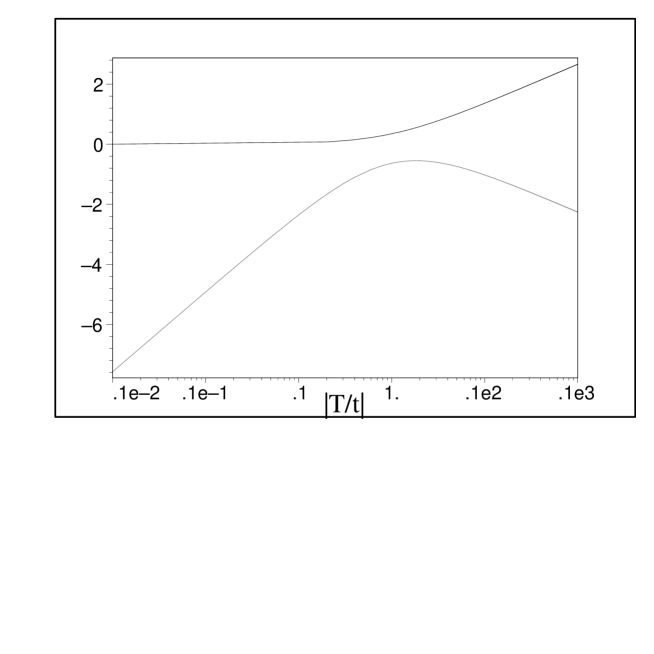
Figure 5: Time-behaviour of $\beta$ (upper curve) and $\varphi$ (lower curve).

At early times, $|t-t_{0}|\gg|T|$, the evolution is basically of power-law type with powers $p_{i}$, because at early time the five-brane is effectively frozen at $z\simeq d+z_{0}$ and does not contribute a substantial amount of kinetic energy. This changes dramatically once we approach the time $|t-t_{0}|\sim|T|$. In a transition period around this time, the brane moves from its original position by a total distance $d$ and ends up at $z\simeq z_{0}$. At the same time, this changes the behaviour of the moduli $\beta$ and $\varphi$ until, at late time $|t|\ll|T|$, they correspond to another rolling radii solution with powers controlled by $p_{f}$. Concretely, the orbifold size described by $\beta$ turns from being approximately constant at early time to expanding at late time, while the Calabi-Yau size controlled by $\varphi$ undergoes a transition from expansion to contraction. We also find that as with the axion case discussed earlier, the solution runs into strong coupling in both asymptotic regions $t-t_{0}\rightarrow-\infty$ and $t-t_{0}\rightarrow 0$ which illustrates our general result.

In Fig. 6 we have shown a particular case which leads to brane collision. The five-brane is initially located at $d+z_{0}\simeq 0.9$ and moves a total distance of $d=1.5$ colliding with the boundary at $z=0$ at the time $|t-t_{0}|/|T|\simeq 1$.

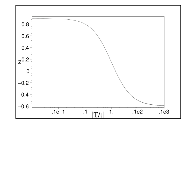
Figure 6: Time-behaviour of the five-brane position modulus $z$ for the example specified in the text. The boundaries are located at $z=0,1$ and the five-brane collides with the $z=0$ boundary at $|t/T|\simeq 1$.

This represents an explicit example of a negative-time branch solution which ends in a small-instanton brane-collision. Solving for these systems has only just the begun, but already interesting features have emerged including a new mechanism for baryogenesis arising from the collision of two branes [50].

9 Summary

In this article we have addressed a number of issues relating to string cosmology. We have seen how rolling radii solutions associated with the low energy string action lead to new inflationary solutions, and how the inclusion of the axion field perturbations can generate scale invariant density fluctuations, although they are primarily isocurvature in nature. The thorny issues of initial conditions and Graceful Exit facing the pre Big Bang scenario have been discussed and possible resolutions proposed. Observational features of string cosmology today have been discussed including gravitational wave detection and anisotropies in the cosmic microwave background. Finally, we have related these solutions to the exciting new solutions arising in M-theory cosmology, and showed how a moving five brane could act in a manner similar to the axion field in the pre Big Bang case. This is an exciting time for string and M-theory cosmology, the subject is developing at a very fast rate, and no doubt there will be new breakthroughs emerging over the next few years. Hopefully out of these we will be in a position to address a number of the issues I have raised in this article, as well as other key ones such as stabilising the dilaton and explaining the current observation of an accelerating Universe.

ACKNOWLEDGEMENTS

I am very grateful to the organisors for inviting me to this wonderful meeting. Following my meeting with him, I would also like to thank Father Christmas for bringing the presents my daughters had asked for.

References

- [1] J. H. Lidsey, D. Wands and E. J. Copeland, Phys. Rep. 337, 343 (2000)
- [2] G. Veneziano, Phys. Lett. B265, 287 (1991)
- [3] M. Gasperini and G. Veneziano. Astropart. Phys. 1, 317 (1993)
- [4] E. J. Copeland, A. Lahiri, and D. Wands, Phys. Rev. D50, 4868 (1994)
- [5] M. D. Pollock and D. Sahdev, Phys. Lett. B222, 12 (1989)
- [6] J. J. Levin and K. Freese, Phys. Rev. D47, 4282 (1993)
- [7] R. Brustein and G. Veneziano, Phys. Lett. B329, 429 (1994)
- [8] M. S. Turner and E. J. Weinberg, Phys. Rev. D56, 4604 (1997)
- [9] D. Clancy, J. E. Lidsey, and R. Tavakol, Phys. Rev. D58, 044017 (1998)
- [10] N. Kaloper, A. D. Linde, and R. Bousso, Phys. Rev. D59, 043508 (1999)
- [11] J. Maharana, E. Onofri, and G. Veneziano, J. High Energy Phys. 01, 004 (1998)
- [12] G. Veneziano, Phys. Lett. B406, 297 (1997)
- [13] A. Buonanno, K. A. Meissner, C. Ungarelli, and G. Veneziano, Phys. Rev. D57, 2543 (1998)
- [14] A. Buonanno, T. Damour, and G. Veneziano, Nucl. Phys. B543, 275 (1999)
- [15] M. Gasperini, Phys. Rev. D61 087301 (2000)
- [16] D. Clancy, J. E. Lidsey, and R. Tavakol, Phys. Rev. D59, 063511 (1999)
- [17] M. Gasperini’s web page, http://www.to.infn.it/ gasperin/
- [18] R. Brustein and R. Madden, Phys. Lett. B410, 110 (1997) R. Brustein and R. Madden, Phys. Lett. B410, 110 (1997)
- [19] R. Brustein and R. Madden, Phys. Rev. D57, 712 (1998) R. Brustein and R. Madden, Phys. Rev. D57, 712 (1998).
- [20] C. Cartier, E. J. Copeland and R. Madden, JHEP 0001, 035 (2000)
- [21] M. Gasperini, M. Maggiore, and G. Veneziano, Nucl. Phys. B494, 315 (1997)
- [22] K.A. Meissner, Phys. Lett. B392, 110 (1997).
- [23] N. Kaloper and K.A. Meissner, Phys. Rev. D56, 7940 (1997)
- [24] R.R. Metsaev and A.A. Tseytlin, Nucl. Phys. B293, 385 (1987)
- [25] J. Khoury, B. A. Ovrut, P. J. Steinhardt and N. Turok, Phys. Rev. D64, 123522 (2001) and hep-th/0108187
- [26] R. Kallosh, L. Kofman and A. Linde, Phys. Rev. D64, 123523 (2001)
- [27] P. J. Steinhardt and N. Turok, hep-th/0111030 and hep-th/0111098
- [28] V. F. Mukhanov, Sov. Phys. JETP 68, 1297 (1988)
- [29] V. F. Mukhanov, H. A. Feldman, and R. H. Brandenberger, Phys. Rep. 215, 203 (1992)
- [30] J. M. Bardeen, P. J. Steinhardt, and M. S. Turner, Phys. Rev. D28, 679 (1983)
- [31] R. Brustein, M. Gasperini, M. Giovannini, V. F. Mukhanov, and G. Veneziano, Phys. Rev. D 51, 6744 (1995)
- [32] E. J. Copeland, R. Easther, and D. Wands, Phys. Rev. D56, 874 (1997)
- [33] A. R. Liddle and D. H. Lyth, Phys. Rep. 231, 1 (1993)
- [34] C. Cartier, E. J. Copeland and M. Gasperini, Nucl. Phys. B607, 406 (2001)
- [35] E. J. Copeland, J. E. Lidsey, and D. Wands, Nucl. Phys. B506, 407 (1997)
- [36] C. Cartier, J. Hwang and E. J. Copeland, Phys. Rev. D64, 103504 (2001)
- [37] R. Durrer, M. Gasperini, M. Sakellariadou, and G. Veneziano, Phys. Lett. B436, 66 (1998)
- [38] R. Durrer, M. Gasperini, M. Sakellariadou, and G. Veneziano, Phys. Rev. D59, 043511 (1999)
- [39] A. Melchiorri, F. Vernizzi, R. Durrer and G. Veneziano, Phys. Rev. Lett. 83, 4464 (1999)
- [40] F. Vernizzi, A. Melchiorri and R. Durrer, Phys. Rev. D63, 063501 (2001).
- [41] K. Enqvist and M. S. Sloth, hep-ph/0109214
- [42] D. Lyth and D. Wands, Phys. Lett. B524, 5 (2002)
- [43] B. Allen and R. Brustein, Phys. Rev. D55, 3260 (1997)
- [44] M. Maggiore, Phys. Rept. 331, 283 (2000)
- [45] E. J. Copeland, A. R. Liddle, J. E. Lidsey, and D. Wands, Phys. Rev. D58, 063508 (1998)
- [46] D. Lemoine and M. Lemoine, Phys. Rev. D52, 1955 (1995)
- [47] M. Gasperini, M. Giovannini, and G. Veneziano, Phys. Rev. Lett. 75, 3796 (1995)
- [48] M. Gasperini, M. Giovannini, and G. Veneziano, Phys. Rev. D52, 6651 (1995)
- [49] E.J. Copeland, J. Gray and A. Lukas, Phys. Rev. D64, 126003 (2001)
- [50] M. Bastero-Gill, E.J. Copeland, J. Gray, A. Lukas, M. Plumacher, hep-th/0201040