Cosmology With Negative Potentials

Abstract:

We investigate cosmological evolution in models where the effective potential $V(\phi)$ may become negative for some values of the field $\phi$. Phase portraits of such theories in space of variables $(\phi,\dot{\phi},H)$ have several qualitatively new features as compared with phase portraits in the theories with $V(\phi)>0$. Cosmological evolution in models with potentials with a “stable” minimum at $V(\phi)<0$ is similar in some respects to the evolution in models with potentials unbounded from below. Instead of reaching an AdS regime dominated by the negative vacuum energy, the universe reaches a turning point where its energy density vanishes, and then it contracts to a singularity with properties that are practically independent of $V(\phi)$. We apply our methods to investigation of the recently proposed cyclic universe scenario. We show that in addition to the singularity problem there are other problems that need to be resolved in order to realize a cyclic regime in this scenario. We propose several modifications of this scenario and conclude that the best way to improve it is to add a usual stage of inflation after the singularity and use that inflationary stage to generate perturbations in the standard way.

1 Introduction

Since the invention of inflationary cosmology [1]-[5], the theory of the evolution of scalar fields in an expanding universe has been investigated quite extensively, both at the classical and the quantum level. While many features of scalar field cosmology are well understood, the overall picture remains somewhat incomplete. In this paper we will extend the investigation of scalar field cosmology to models with negative effective potentials. We are also going to bring together several other issues, such as the impact of radiation and particle production on the onset of inflation. This will allow us to get a better understanding of various possibilities that may appear in scalar field cosmology.

We are going to use a general approach based on the investigation of 3d phase portraits that show the behavior of the scalar field $\phi$, its velocity $\dot{\phi}$, and the Hubble constant $H={\dot{a}\over a}$. We will see that the phase portraits of models with $V(\phi)>0$ and with $V(\phi)<0$ are qualitatively different and that additional changes appear when one adds matter and/or radiation.

There are several reasons to study cosmology with negative potentials. The first one is related to the cosmological constant problem. The simplest potential used in inflationary cosmology is $V(\phi)={1\over 2}m^{2}\phi^{2}$ [4]. One can add to this potential a small cosmological constant $V_{0}$ without changing any features of inflation. A small positive $V_{0}\sim 10^{-120}$ (in Planck units) would be sufficient to describe the present acceleration of the universe in a de Sitter-like state. But why should $V_{0}$ be so small and positive? What would happen for $V_{0}<0$? Does the post-inflationary universe with $V_{0}<0$ behave like anti-de Sitter space, which is so popular in M-theory?

Rather unexpectedly, the answer to this question appears to be negative: After a long stage of inflation the universe with $V_{0}<0$ cannot approach an AdS regime; instead of that it collapses [6, 7, 8]. In this paper we will study cosmological behavior in a large class of theories with negative potentials and explain why the universe in these theories stops expanding and eventually collapses.

Another reason to study theories with negative potentials is provided by the investigation of cosmology in N=2,4,8 gauged supergravity. Recently it was found that in all known versions of these theories potentials with extrema at $V(\phi)>0$ are unbounded from below. Despite this fact, such models can, under certain conditions, describe the present stage of acceleration of the universe [7, 8].

One more reason is related to a formal connection with warp factor/bulk scalar dynamics in brane cosmology. It has recently been shown that the equations for the warp factor and scalar field in brane cosmology with a scalar field potential $V(\phi)$ are similar to the equations for the scale factor and scalar field in 4D cosmology with the opposite potential $-V(\phi)$ [9]. This reveals an interesting relation of cosmology with negative potentials and warp geometry with positive potentials.

Finally, cosmology with a negative potential $V(\phi)$ is the basis of the recently proposed “cyclic universe” model [10] based in part on the ekpyrotic scenario [11]. However, unlike in the ekpyrotic scenario [11], the authors of [10] assume, in accordance with [12], that the scalar field potential $V(\phi)$ at large $\phi$ is positive and nearly constant. As a result, the universe experiences “superluminal expansion” (inflation) that helps to solve some of the cosmological problems. In this sense cyclic scenario, unlike the ekpyrotic scenario of Ref. [11], is a specific version of inflationary theory rather than an alternative to inflation. Then the scalar field rolls to a minimum of its effective potential with $V(\phi)<0$, the universe contracts to a singularity, re-emerges and again enters a stage of inflation. This scenario inherits many unsolved problems of the ekpyrotic model [12], including the singularity problem [13]. The authors assume that the universe can pass through the singularity and that one can use perturbation theory and specific matching conditions at the singularity to calculate density perturbations in the post-big bang universe generated by processes prior to the singularity [14]. This issue is rather controversial [15]. The possibility of achieving a cyclic regime depends on various assumptions concerning the creation of matter and the acceleration of the scalar field during the big bang.

The idea that the big bang is not the beginning of the universe but a point of a phase transition is quite interesting, see e.g. [16]-[22]. However, the more assumptions about the singularity one needs to make, the less trustworthy are the conclusions. In this respect, inflationary theory provides us with a unique possibility to construct a theory largely independent of any assumptions about the initial singularity. According to this theory, the structure of the observable part of the universe is determined by processes at the last stages of inflation, at densities much smaller than the Planck density. As a result, observational data practically do not depend on the unknown initial conditions in the early universe.

Since the cyclic scenario does require repeated periods of inflation anyway, it would be nice to avoid the vulnerability of this scenario with respect to the unknown physics at the singularity by placing the stage of inflation before the stage of large scale structure formation rather than after it.

In order to achieve this goal we will examine the conditions that are necessary for the existence of the cyclic regime in the model of Ref. [10] and then check whether the model can be modified in a way that would not require various speculations about the behavior of matter, the scalar field, and density perturbations near the singularity.

Our paper will thus consist of two parts. The first part will contain a general study of scalar field cosmology with positive and negative potentials. The second part will be devoted to a more speculative subject, it will include application of our general results to the cyclic scenario.

In Section 2 we will describe several basic regimes that are possible in scalar field cosmology: the universe can be dominated by potential energy, by kinetic energy, by the energy density of an oscillating scalar field, or by matter or radiation. The discussion of these four distinct regimes will help us to understand the phase portraits of the universe that we are going to draw in the subsequent sections.

Section 3 will describe the use of phase portraits for studying cosmological evolution. We will write the evolution equations for the field and scale factor in the form of three first order equations plus one time dependent constraint. The solutions to these equations can then be represented as trajectories in phase space, clearly showing the possible ways the universe can evolve in different situations. Finally, by using a Poincaré projection we can map the entire phase space onto a finite sphere, thus allowing the complete set of possible trajectories to be easily seen.

In Section 4 we will apply these methods to models with positive definite potentials. Such potentials have been extensively studied before with the use of phase portraits [23, 24]. We study them here partly to introduce the methods we are using and to provide a point of comparison for the negative potentials of the following section. We also present some new results concerning the effects of matter and radiation on the development of inflation.

In Section 5 we show the phase portraits for a model where the effective potential can become negative. We discuss general properties of such models, and in particular the ways in which they differ from the models of the previous section. One of our major conclusions is that such models generically enter a stage of contraction. In Section 6 we will examine in detail the transition from expansion to contraction in models of this type.

Many of the features of scalar field cosmology that we are going to discuss are model-independent. The phase portraits in Sections 4-6 all use the simplest model $V(\phi)=m^{2}\phi^{2}/2+V_{0}$, but in Section 7 we discuss some other theories with negative potentials.

In Section 8 we will discuss cosmological evolution near the initial and final singularities, and in particular the role of particle production and anisotropy near the singularity.

In Section 9 we will apply our methods to the investigation of the cyclic scenario. As we will see, the cyclic regime in this scenario does not appear automatically. One should fine-tune the potential $V(\phi)$ and learn how to work with the super-Planckian potentials $|V(\phi)|>1$. One should also introduce superheavy particles with specific properties, study their production at the singularity, and make sure that they do not affect the present stage of the evolution of the universe. This adds new “epicycles” to this scenario, making it even more speculative. We discuss several possible modifications of this scenario and conclude that the best way to improve it is to add a usual stage of inflation before the stage of large scale structure formation. This modification resolves many problems of the original version of the cyclic scenario. In this modified form of the cyclic scenario inflation is once again the source of density perturbations as well as the resolution of the cosmological problems such as homogeneity and flatness.

Section 10 summarizes our main conclusions concerning cosmology with negative potentials and cyclic universe.

2 Four Basic Regimes in Scalar Field Cosmology

2.1 A toy model with $V(\phi)={1\over 2}m^{2}\phi^{2}+V_{0}$

We will study the behavior of a homogeneous scalar field in a Friedmann universe with the metric

$$ds^{2}=-dt^{2}+a^{2}(t)ds_{3}^{2}\ ,$$ (1)

where $ds_{3}^{2}=\gamma_{ij}dx^{i}dx^{j}$ is the metric of a 3d space with constant curvature, $k=0,\pm 1$.

In this paper we will use a system of units in which $M_{p}=1$, where $M_{p}=(8\pi G)^{-1/2}\sim 2\times 10^{18}$ GeV. The Friedmann equation for a scalar field with potential energy density $V(\phi)$ is

$$H^{2}=\left({\dot{a}\over a}\right)^{2}={1\over 3}\rho-{k\over a^{2}}={1\over 3}\left({1\over 2}\dot{\phi}^{2}+V(\phi)+\rho_{\alpha}\right)-{k\over a^{2}}\ .$$ (2)

Here $\rho$ is the total energy density and $\rho_{\alpha}$ is the density of matter with equation of state $p_{\alpha}=\alpha\rho_{\alpha}$. For non-relativistic matter $\alpha=0$, while for radiation $\alpha=1/3$.

The evolution of $H$ is given by a combination of the Einstein equations

$$\dot{H}=-{1\over 2}(\rho+p)+{k\over a^{2}}=-{1\over 2}(\dot{\phi}^{2}+\rho_{\alpha}(1+\alpha))+{k\over a^{2}}\ .$$ (3)

Alternatively, one can use the equation

$${\ddot{a}\over a}=-{1\over 6}(\rho+3p)={1\over 3}(V(\phi)-\dot{\phi}^{2})-{1\over 6}\rho_{\alpha}(1+3\alpha)\ .$$ (4)

The evolution of the scalar field $\phi$ follows from the Einstein equations,

$$\ddot{\phi}+3H\dot{\phi}+V_{,\phi}=0\ .$$ (5)

We shall study the basic properties of scalar field cosmology using as an example the simplest harmonic oscillator potential

$$V(\phi)={1\over 2}m^{2}\phi^{2}+V_{0}\ ,$$ (6)

Surprisingly, we will find that cosmology with the potential (6) with $V_{0}<0$ shares some common features with the cosmology of the “inverse” harmonic oscillator potential

$$V(\phi)=-{1\over 2}m^{2}\phi^{2}-V_{0}\ .$$ (7)

In particular, the expansion of the universe in theories with $V_{0}<0$ always turns into cosmological contraction.

Constructing phase portraits is a powerful method for investigating the dynamics of the scale factor/scalar field system (3)-(5). Before we look at the phase portraits for various values of $V_{0}$ in this model, it will be useful to discuss some of their features. For the remainder of this section we will consider $k=0$, i.e. flat universes. While this case will be the main focus of our discussion throughout the paper, we will in several cases refer to the extension of our results to open or closed universes as well.

There are four basic regimes that we may encounter: the universe can be dominated by the potential energy density $V(\phi)$, by the kinetic energy density $\dot{\phi}^{2}/2$, by the energy density of an oscillating scalar field, in which case $V(\phi)\sim\dot{\phi}^{2}/2$, or by matter/radiation $\rho_{\alpha}$.

2.2 The inflationary regime: Energy density dominated by $V(\phi)$

Inflation occurs when the energy density is dominated by $V(\phi)$. In this case $\dot{\phi}^{2}/2,\rho_{\alpha}\ll V(\phi)$ and $|\ddot{\phi}|\ll|3H\dot{\phi}|$. This corresponds to the vacuum-like equation of state

$$p=-\rho\ .$$ (8)

The equations for $a$ and $\phi$ in this regime have the following form:

$$H^{2}=\left({\dot{a}\over a}\right)^{2}={{m^{2}\phi^{2}}\over 6}+{V_{0}\over 3}\ ,$$ (9)

$$3{\dot{a}\over a}\dot{\phi}+m^{2}\phi=0\ .$$ (10)

The solutions of the equations for $\phi(t)$ and $a(t)$ for the most interesting case ${m^{2}\phi^{2}\over 2}\gg|V_{0}|$ are given by [4, 25]

$$\phi(t)=\phi_{0}-\sqrt{2\,\over 3}{mt}~{},$$ (11)

$$a(t)=a_{0}\,\exp\left(\frac{\phi_{0}^{2}-\phi^{2}(t)}{4}\right)\,~{}.$$ (12)

These solutions, which describe inflationary expansion, are valid only for $\dot{\phi}^{2}/2\ll V(\phi)$, which implies that inflation ends at

$$|\phi_{e}|\sim 1~{}.$$ (13)

In this paper we will assume that $m^{2}\gg|V_{0}|$, in which case ${m^{2}\phi^{2}\over 2}\gg|V_{0}|$ is always satisfied during inflation.

Note that the same solution is valid if one reverses the time arrow, $t\to-t$, in which case it describes a quasi-exponential contraction of the universe (deflation).

2.3 The kinetic regime: Energy density dominated by $\dot{\phi}^{2}/2$

Another important regime occurs when the energy density is dominated by $\dot{\phi}^{2}/2$. In this case $V(\phi),\rho_{\alpha}\ll\dot{\phi}^{2}/2$ and $|\ddot{\phi}|,|3H\dot{\phi}|\gg m^{2}\phi$. This corresponds to the “stiff” equation of state

$$p=\rho\ .$$ (14)

The equations for $a$ and $\phi$ are:

$$H^{2}=\left({\dot{a}\over a}\right)^{2}={{\dot{\phi}^{2}}\over 6}\ ,$$ (15)

$${\ddot{\phi}\over\dot{\phi}}=-3{\dot{a}\over a}\ .$$ (16)

The solutions can be written as follows:

$$a(t)=t^{1/3}~{},$$ (17)

$$\phi=\phi_{0}\pm\sqrt{2\over 3}\ \ln{t_{0}\over t};\qquad{\dot{\phi}^{2}\over 2}={1\over 3t^{2}}\ .$$ (18)

These solutions can describe an expanding universe or a universe collapsing towards a singularity.

During the expansion of the universe, the inflationary regime $V(\phi)\gg\dot{\phi}^{2}/2$ represents a stable intermediate asymptotic attractor. Even if a flat universe begins in a state with $\dot{\phi}^{2}/2\gg V(\phi)$, it typically rapidly switches to an inflationary regime with $V(\phi)\gg\dot{\phi}^{2}/2$ [23, 24, 26]. This occurs because during the expansion of the universe with $\dot{\phi}^{2}/2\gg V(\phi)$, the value of the kinetic energy drops down like $t^{-2}$, whereas the field changes only logarithmically. Therefore for all power-law potentials, the value of $V(\phi)$ decreases much more slowly than $\dot{\phi}^{2}/2$. When it becomes greater than $\dot{\phi}^{2}/2$, inflation begins.

During the collapse of the universe, the opposite occurs. $V(\phi)$ grows only logarithmically, whereas $\dot{\phi}^{2}/2$ diverges as $t^{-2}$, where $t$ is the time remaining before the big crunch singularity. This means that the regime $\dot{\phi}^{2}/2\gg V(\phi)$ generically occurs at the stage of collapse. In this regime one can neglect $V(\phi)$ in the investigation of the singularity at $t\to 0$.

2.4 The oscillatory regime: Evolution determined by the energy density of an oscillating scalar field

Now let us assume that the field $\phi$ oscillates near $\phi=0$ with frequency much greater than $H$, and that the average value of $V(\phi)$ during these oscillations is much greater than $V_{0}=V(0)$. In this case one can neglect the term $3H\dot{\phi}$ in Eq. (5), so that in the first approximation one simply has

$$\ddot{\phi}+m^{2}\phi=0$$ (19)

and

$$\phi=\Phi~{}\sin mt\ .$$ (20)

Here $\Phi$ is the amplitude of the oscillation. The pressure $p=\dot{\phi}^{2}/2-V(\phi)$ produced by these oscillations is given by ${m^{2}\over 2}\Phi^{2}~{}\cos 2mt$, so if one takes an average over many oscillations, the pressure vanishes, $p\approx 0$. The universe in this regime expands as $a\sim t^{2/3}$. Since the total energy of pressureless matter is conserved, the amplitude of the oscillations decreases, $\Phi(t)\sim a^{-3/2}\sim t^{-1}$.

The regime of oscillations usually begins after the end of inflation, at $\phi\mathrel{\hbox{\hbox to0.0pt{\hbox{\lower 4.0pt\hbox{$\sim$}}\hss}\hbox{$<$}}}1$. As long as one can neglect $V_{0}$, the field oscillations after inflation approach the following asymptotic regime [27]:

$$\phi(t)\approx{2\sqrt{2}\over\sqrt{3}~{}mt}\,\sin\,mt~{}\approx~{}{\sqrt{2}\over\pi\sqrt{3}~{}N}\,\sin\,mt\ .$$ (21)

Here $t$ is the time after the end of inflation and $N$ is the number of oscillations.

Figure 1: Evolution of the scalar field and the scale factor in the model $V(\phi)={m^{2}\over 2}\phi^{2}+V_{0}$ with $V_{0}>0$. In the beginning we have a stage of inflation with the field $\phi$ linearly decreasing at $\phi>1$. At this stage the equation of state is $p\approx-\rho$. Then the field enters a stage of oscillations with a gradually decreasing amplitude of the field; $p\ll\rho$. When the energy of the oscillations becomes smaller than $V_{0}$, the universe enters a second stage of inflation.

It is amazing that this simple model with $V_{0}>0$ can describe not only inflation in the early universe, but also the present stage of inflation/acceleration. Indeed, when the amplitude becomes very small the term $V_{0}$ will become important, and the universe enters a second stage of inflation with $H^{2}=V_{0}/3$. The amplitude of oscillations of the field $\phi$ in this regime falls down exponentially. In particular, for $m^{2}\gg H^{2}$ the amplitude decreases as $e^{-3Ht/2}$. The evolution of the scalar field and the scale factor in the theory with $V_{0}>0$ is shown in Fig. 1.

Meanwhile, if one considers the model with $V_{0}<0$, a dramatic change occurs when the energy density of oscillations (and matter) gradually decreases and becomes comparable to $-V_{0}$. According to Eqs. (2) and (3), the expansion of the universe slows down at that time, and eventually the universe begins collapsing, see Fig. 2.

Figure 2: Evolution of the scalar field and the scale factor in the model $V(\phi)={m^{2}\over 2}\phi^{2}+V_{0}$ with $V_{0}<0$. In the beginning we have a stage of inflation with the field $\phi$ linearly decreasing at $\phi>1$. At this stage the equation of state is $p\approx-\rho$. Then the field enters a stage of oscillations with a gradually decreasing amplitude of the field; $p\ll\rho$. When the energy of the oscillations becomes equal to $|V_{0}|$, the universe stops expanding and begins to contract. At this stage the amplitude of oscillations grows. When it becomes greater than $O(1)$, the field stops oscillating, the energy density is dominated by the kinetic energy of the scalar field, $p\approx\rho$, and the universe collapses.

When the universe contracts, the amplitude of oscillations grows as $a^{-3/2}$. However, this process does not continue too long. Indeed, let us compare $3H\dot{\phi}$ and $m^{2}\phi$ in this regime. If one can neglect $V_{0}$ (and this is always the case for a sufficiently large $\Phi$), one has $H\approx m\Phi/\sqrt{6}$ and $\dot{\phi}\sim m\phi$. Therefore one has $|3H\dot{\phi}|\gg|m^{2}\phi|$ for $\phi\gg 1$, so instead of Eq. (20) one should use Eq. (16). Thus, during the collapse of the universe the stage of oscillations ends and the regime dominated by kinetic energy begins at

$$|\phi_{b}|\sim 1~{}.$$ (22)

Note that $|\phi_{b}|\sim|\phi_{e}|$, see Eq. (13).

We will study the switch from expansion to contraction in a flat universe in a much more detailed way in Section 6. However, we would like to make here some comments concerning this process.

The general textbook wisdom is that open and flat universes expand forever, whereas closed universes eventually collapse. This lore was based on investigation of universes with vanishing cosmological constants. A closed universe with a sufficiently large positive cosmological constant may expand forever, whereas open and flat universes with a negative cosmological constant eventually collapse.

One of the well-known solutions of this type is an open universe with a negative vacuum energy $V_{0}$. There is a solution to the Friedmann equation $H^{2}-a^{-2}=V_{0}/3$ for $V_{0}<0$:   $a(t)=\sqrt{3\over|V_{0}|}~{}\sin\sqrt{|V_{0}|\over 3}\,t$. This is a specific section of anti de Sitter space, which is popular in M-theory and brane cosmology. This universe has a coordinate singularity at $t=\pi\sqrt{3\over|V_{0}|}$. Naively, one might think that this is exactly what we have found in our investigation of universes with $V_{0}<0$, namely that when the energy density of matter in an expanding universe decreases and the total energy density becomes dominated by a negative cosmological constant, our universe reaches an AdS regime dominated by a negative cosmological constant.

However, this is not the case. We discuss here a flat universe regime, which appears after a long stage of inflation. In this case (unless one considers open inflation models with $\Omega<1$) the term ${k\over a^{2}}$ with $k=\pm 1,0$ can be omitted in the general Friedmann equation. The Friedmann equation $H^{2}=\rho/3$ describing a flat universe does not have any solutions with $\rho(\phi)<0$. Once the universe approaches the turning point where the total energy density vanishes it begins collapsing, and the total energy density becomes positive again [6, 7, 8]. Thus the standard inflationary prediction $\Omega=1$ implies that we cannot live in AdS space dominated by a negative cosmological constant [7, 8].

2.5 Evolution determined by the energy density of matter or radiation

The first models of inflation were based on the assumption that the universe from the very beginning was in a state of thermal equilibrium; inflation began when the temperature of the universe became much smaller than the Planck temperature $T\sim M_{p}$ [2, 3]. Later it was found that this assumption is not necessary, and in many models inflation may start immediately after the big bang [4]. In this case the existence of matter prior to inflation becomes less important, and sometimes it even hampers the development of inflation [25]. Therefore many works on initial conditions for inflation neglect the possible impact of matter on the motion of the scalar field and concentrate on finding self-consistent cosmological solutions describing scalar fields in otherwise empty universes. This is the simplest approach, especially in cases where $\dot{\phi}^{2}/2\ll V(\phi)$ and inflation begins immediately after the big bang.

However, in some cases the scalar field initially may have large kinetic energy, $\dot{\phi}^{2}/2\gg V(\phi)$. Moreover, one may expect creation of relativistic or non-relativistic particle near the singularity. Note that the existence of even a small amount of matter may have an important effect on the motion of the field. Indeed, the kinetic energy of the scalar field $\dot{\phi}^{2}/2$ in the regime $\dot{\phi}^{2}/2\gg V(\phi)$ decreases as $a^{-6}$. Meanwhile, the density of radiation decreases as $a^{-4}$ and the density of non-relativistic matter decreases as $a^{-3}$. Therefore the energy density of matter eventually becomes greater than $\dot{\phi}^{2}/2$. As we will see, once it occurs, the field rapidly slows down or even completely freezes. This effect may provide good initial conditions for a subsequent stage of inflation [28].

Indeed, let us assume that in the beginning the field $\phi$ moves very fast, so that $|3H\dot{\phi}|\gg|V,_{\phi}|=|m^{2}\phi|$. Suppose, however, that at some moment the energy density of the universe becomes dominated by matter with the equation of state $p_{\alpha}=\alpha\rho_{\alpha}$. In this regime one can represent the cosmological evolution in the following form [25]

$$\rho_{\alpha} = \rho_{\alpha}(t_{0})\left({a(t)\over a_{0}}\right)^{-3(1+\alpha)},$$

$$a(t) = a_{0}\left({t\over t_{0}}\right)^{2\over 3(1+\alpha)},$$

$$H = {2\over 3(1+\alpha)t}~{},$$

$$\dot{\phi} = \dot{\phi}_{0}{a_{0}^{3}\over a^{3}}=\dot{\phi}_{0}\left({t_{0}\over t}\right)^{2\over 1+\alpha}~{}.$$ (23)

This regime has a very interesting feature: Even if it continues for an indefinitely long time, the change of the field $\phi$ during this time remains quite limited. Indeed,

$$\Delta\phi\leq\int\limits_{t_{0}}^{\infty}\dot{\phi}dt=\dot{\phi}_{0}\int\limits_{t_{0}}^{\infty}\left({t_{0}\over t}\right)^{2\over 1+\alpha}dt={1+\alpha\over 1-\alpha}~{}\dot{\phi}_{0}t_{0}.$$ (24)

If $t_{0}$ is the very beginning of matter domination ($\dot{\phi}_{0}^{2}/2\sim\rho_{\alpha}$), then $\dot{\phi}_{0}t_{0}\sim{2\over\sqrt{3}(1+\alpha)}=O(1)$. Therefore

$$\Delta\phi\mathrel{\hbox{\hbox to0.0pt{\hbox{\lower 4.0pt\hbox{$\sim$}}\hss}\hbox{$<$}}}1$$ (25)

in Planck units (i.e. $\Delta\phi\mathrel{\hbox{\hbox to0.0pt{\hbox{\lower 4.0pt\hbox{$\sim$}}\hss}\hbox{$<$}}}M_{p}$). This means, in particular, that a free field $\phi$ in a matter dominated universe cannot move by more than $O(M_{p})$.

This simple result has important implications. In particular, if the motion of the field in a matter-dominated universe begins at $|\phi|\gg 1$, then it can move only by $\Delta\phi\mathrel{\hbox{\hbox to0.0pt{\hbox{\lower 4.0pt\hbox{$\sim$}}\hss}\hbox{$<$}}}1$. Therefore in theories with flat potentials the field always remains frozen at $|\phi|\gg 1$.

The field begins moving again only when the Hubble constant decreases and $|3H\dot{\phi}|$ becomes comparable to $|V,_{\phi}|$. But in this case the condition $3H\dot{\phi}\approx|V,_{\phi}|$ automatically leads to inflation in the theory $m^{2}\phi^{2}/2+V_{0}$ for $|V_{0}|<m^{2}$ and $\phi\gg 1$.

This means that even a small amount of matter or radiation may increase the chances of reaching a stage of inflation, see [28] and Fig. 5 in Section 5. Indeed, consider any theory with $V(\phi)\sim\phi^{n}$. Suppose in the beginning we had a kinetic energy dominated regime $\dot{\phi}^{2}/2\gg\rho_{\alpha},V(\phi)$ starting at $\phi\gg 1$. Then the field $\phi$ would change very slowly, whereas $\dot{\phi}^{2}/2$ would rapidly drop down until it became comparable either to $V(\phi)$ or to $\rho_{\alpha}$. If at that moment $V(\phi)>\rho_{\alpha}$, inflation would begin immediately. But even in the most unfavorable case $V(\phi)\ll\rho_{\alpha}$ inflation would begin eventually. Indeed, at $\phi\gg 1$ one has the double inequality $m^{2}=V^{\prime\prime}\ll V(\phi)\ll\rho_{\alpha}\sim H^{2}$. Therefore the Hubble constant is much greater than the effective scalar field mass. In this case the field practically does not move until the desirable regime $V(\phi)>\rho_{\alpha}$ is reached and inflation begins.

3 Phase Portraits and Cosmological Evolution

Having discussed some important limiting regimes in scalar field cosmology, we are now ready to investigate the complete evolution of a Friedmann universe with a scalar field. Later we will discuss the effects of adding matter to this system, but for now we restrict ourselves to a system with three independent variables, $\phi$, $\dot{\phi}$, and $H$. To study this system we find it most convenient to rewrite the evolution equations for $a$ and $\phi$ as a set of three coupled, first-order, differential equations:

$${d\phi\over dt} = \dot{\phi}$$ (26)

$${d\dot{\phi}\over dt} = -3H\dot{\phi}-V_{,\phi}$$ (27)

$${dH\over dt} = -{1\over 3}\left(\dot{\phi}^{2}-V\right)-H^{2}$$ (28)

plus the constraint equation

$$H^{2}-{1\over 6}\dot{\phi}^{2}-{1\over 3}V=-{k\over a^{2}}.$$ (29)

All solutions to these three equations can be represented as trajectories in the 3d phase space of $\phi$, $\dot{\phi}$, and $H$. Simply looking at plots showing a number of these trajectories can help give some intuition for the cosmology of a particular model (as defined by the potential $V$). There are a number of ways to get more information out of the phase portraits, however.

One important step is to determine all of the critical points, i.e. the points for which the derivatives of all three phase variables vanish. There are finite and infinite critical points. Every trajectory must begin and end at these critical points.

To find infinite critical points and visualize the flow of trajectories at infinity, a useful trick is to do a Poincaré mapping

$$x_{P}\equiv{x\over 1+r}\ ,$$ (30)

where $x$ is any of ($\phi$, $\dot{\phi}$, $H$) and $r^{2}=\phi^{2}+\dot{\phi}^{2}+H^{2}$. The interior of the unit sphere $\phi_{P}^{2}+\dot{\phi}_{P}^{2}+H_{P}^{2}=1$ maps to the infinite phase space of $\phi$, $\dot{\phi}$, and $H$, so by plotting trajectories in these new coordinates the entire phase space can be easily visualized. At times in this paper we will plot a 2d phase portrait, e.g. in the variables $\phi$ and $\dot{\phi}$ only. In these cases we use a 2d Poincaré mapping where $r^{2}=\phi^{2}+\dot{\phi}^{2}$.

With the Poincaré mapping it is possible to identify a set of infinite critical points, namely those that occur on the bounding sphere $\phi_{P}^{2}+\dot{\phi}_{P}^{2}+H_{P}^{2}=1$. These points represent the possible starting and ending points for all trajectories that go off to infinity in the usual coordinates.

Because no two trajectories can ever cross in phase space, it is easy to define the behavior of a system whose phase portrait is two dimensional. Fortunately, for the cosmological systems we are considering we can identify a 2d surface that separates different regions of the 3d phase space. For the flat universe $k=0$ the constraint equation (29) defines a 2d surface. All trajectories in this case are located at this surface, i.e. the phase portrait for the flat universe is two dimensional. This surface in turn divides the phase space into three separate regions (including the surface itself) representing the possible types of curvature. No trajectory can pass from one of these regions to another. Although the location of the finite critical points for a given model depends strongly on $V$, the structure of the infinite critical points is very similar across a wide range of potentials. See [9] for recent discussion.

4 Cosmology with a Non-Negative Potential

As a simple example we consider the model $V(\phi)=V_{0}+{1\over 2}m^{2}\phi^{2}$ discussed in Section 2.1. By rescaling the field and time variables the mass $m$ can be eliminated from the equations, so for simplicity we simply set $m=1$ in what follows. Thus the evolution and constraint equations become

$${d\phi\over dt} = \dot{\phi}$$ (31)

$${d\dot{\phi}\over dt} = -3\dot{\phi}H-\phi$$ (32)

$${dH\over dt} = -{1\over 3}\dot{\phi}^{2}+{1\over 6}\phi^{2}+{1\over 3}V_{0}-H^{2}$$ (33)

$$6H^{2}-\dot{\phi}^{2}-\phi^{2}-2V_{0}=-6{k\over a^{2}}.$$ (34)

The hypersurface representing a flat universe is given by setting $k=0$ in the constraint equation, which gives

$$6H^{2}-\dot{\phi}^{2}-\phi^{2}=2V_{0}.$$ (35)

The surface defined by this equation is a hyperboloid. For positive definite potentials $V_{0}>0$ it is a hyperboloid of two sheets, meaning the two branches at $H>0$ and $H<0$ are disconnected. For $V_{0}=0$ this hyperboloid reduces to a double cone.

There are two finite critical points for this system at $\phi=\dot{\phi}=0$, $H=\pm\sqrt{V_{0}/3}$. For $V_{0}=0$ these two points reduce to a single finite critical point at the origin. To find the infinite critical points we first rewrite the evolution equations in terms of the Poincaré variables and then set their derivatives equal to zero. This yields eight points.

Figure 3 shows the phase space for this model with $V_{0}>0$ along with a sample of trajectories for $k=0$. The hyperboloid along which all of these trajectories lie represents a flat universe. The upper branch corresponds to expansion and the lower one to contraction. The fact that the two branches are disconnected means that in a flat universe in this model expansion can never reverse and become contraction. Note that this conclusion is unchanged for the case $V_{0}=0$. In that case the hyperboloid becomes a double cone and the two branches touch at a single point. Since that point is a critical point, however, no trajectories can pass from one branch of the cone to the other. The lower branch corresponds to the upper branch with time reversal $t\to-t$. The upper branch of the flat universe hyperboloid is shown projected into a 2d plot in Figure 4. This plot is very similar to the one shown in [23] for this model with $V_{0}=0$.

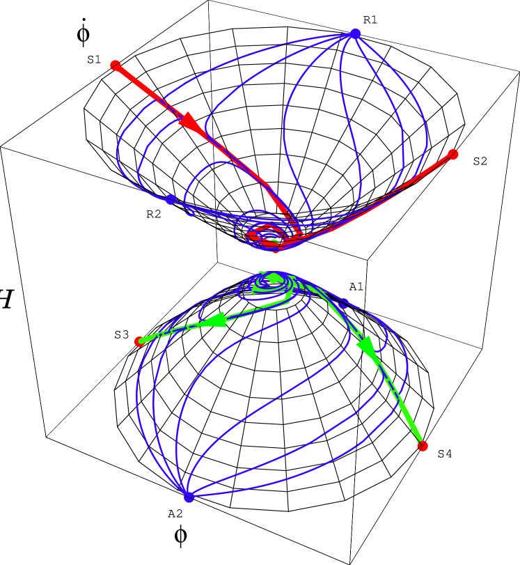
Figure 3: Phase portrait for the theory $V(\phi)={1\over 2}m^{2}\phi^{2}+V_{0}$ with $V_{0}>0$ in rescaled coordinates $(\phi,\dot{\phi},H)$. The branches describing stages of expansion and contraction (upper and lower parts of the hyperboloid) are disconnected.

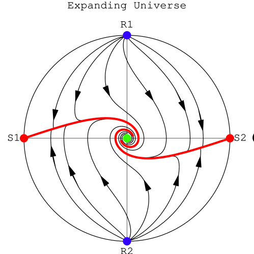
Figure 4: Projection of the upper branch of the full phase portrait for the theory $V(\phi)={1\over 2}m^{2}\phi^{2}+V_{0}$ with $V_{0}>0$ in rescaled coordinates $(\phi,\dot{\phi})$.

For an expanding universe there are four infinite critical points, two repulsors labeled $R_{1}$ and $R_{2}$ and two saddle points labeled $S_{1}$ and $S_{2}$. All trajectories begin at $R_{1}$, $R_{2}$ and wind towards the focus at the center. The separatrices emanating from $S_{1}$ and $S_{2}$ represent attractor trajectories (not to be confused with attractor critical points). Along these trajectories the universe experiences inflation ($\phi^{2}\gg\dot{\phi}^{2}$) until it nears the center and begins winding around it, corresponding to field oscillations near the potential minimum. These separatrices represent a set of measure zero in the space of trajectories; the two shown are the only trajectories that begin at the saddle points. Nonetheless they are important because most of the trajectories emanating from the repulsor points asymptotically approach the separatrices. This is why inflation is a generic feature of models such as this one, and also why inflation erases all information about the initial conditions that preceded it.

Thus a typical trajectory passes through three of the four regimes described in Section 2. Near the repulsors the kinetic energy dominates and the equation of state is stiff, $p\approx\rho$. Near the main part of the separatrices the equation of state is inflationary, $p\approx-\rho$. Finally near the center the scalar field oscillates and the equation of state is that of non-relativistic matter, $p\ll\rho$. During the oscillations the scalar field decreases as

$$\phi(t)\approx{1\over{4N}}\,\sin\,mt\ ,$$ (36)

where $N$ is the number of oscillations, see Eq. (21). Although particle production is not included in these phase portraits, this evolution will typically end with the scalar field decaying into other forms of matter, thus finishing the evolution in the fourth regime, matter and/or radiation domination. The contracting branch is a mirror image of the expanding one, with the same three regimes occurring in the opposite order, finally ending with a big crunch singularity at the attractor points $A_{1}$ and $A_{2}$.

For an open or closed universe the trajectories would lie in the interior or exterior of the hyperboloid, respectively [23]. For an open universe nearly all trajectories would asymptotically approach the separatrices on the flat universe hypersurface. This tendency reflects the fact that for most initial conditions inflation will occur and drive the universe towards flatness. Once this has occurred the trajectories spiral in towards the focus at the bottom of the hyperboloid. For a closed universe there are also many trajectories that rapidly approach these separatrices, but there is also a class of trajectories that moves from the repulsive critical points to the attractive ones without ever passing near the flat universe hypersurface. These trajectories reflect closed universes that collapse rapidly before inflation has a chance to occur.

Figure 5: Phase portrait for the theory $V(\phi)={1\over 2}m^{2}\phi^{2}$ without Poincaré mapping. The blue (thick) lines show trajectories describing the universe without radiation. The scalar field has half Planck density at the beginning of the simulations. The red (thin) lines show trajectories where an equal amount of energy in radiation was added to the system. As we see, in the presence of radiation the velocity of the scalar field rapidly decreases, which usually leads to the onset of inflation.

This conclusion becomes even more apparent if one takes into account matter/radiation [28]. As we have argued in Section 2.5, the existence of matter rapidly freezes the motion of the scalar field. Therefore if the field $\phi$ was initially large and had a large velocity such that $\phi\gg 1$, $\dot{\phi}^{2}/2\gg V(\phi)$, then the presence of matter would increase the probability of inflation. This can be confirmed by comparing the phase portraits of the universe with and without radiation. Although the phase portrait with radiation is three dimensional, it is convenient to make its projection to the $(\dot{\phi},\phi)$ plane, see Fig. 5.

In the second and fourth quadrants of this figure the field starts out moving towards the minimum. The presence of radiation slows the field down, causing it to move more quickly towards the inflationary separatrix trajectory. In the first and third quadrants where the field starts out moving away from the minimum the duration of inflation is slightly diminished by the presence of radiation, but the probability of inflation is nearly unity.

5 Cosmology with a Negative Potential

Now we turn to the main subject of our investigation, cosmological models with scalar field potentials that may become negative. We will continue using the simple example $V(\phi)=V_{0}+{1\over 2}m^{2}\phi^{2}$, but now we will consider $V_{0}<0$. The hypersurface representing a flat universe is still defined by

$$6H^{2}-\dot{\phi}^{2}-\phi^{2}=2V_{0},$$ (37)

but with $V_{0}$ negative, this surface is a hyperboloid of one sheet.

Figure 6 shows the phase space for this model and sample trajectories for a flat universe. The phase space is two dimensional, but its topology is very different from that for non-negative potentials. The infinite critical points are unchanged because the finite term $V_{0}$ has no effect at infinity, but there are no finite critical points. Thus all trajectories begin at infinity with $H>0$ and end at infinity with $H<0$. This is possible because the regions corresponding to expansion and contraction are now connected. This property is valid for all types of curvature $k$, i.e. for open, flat or closed universes.

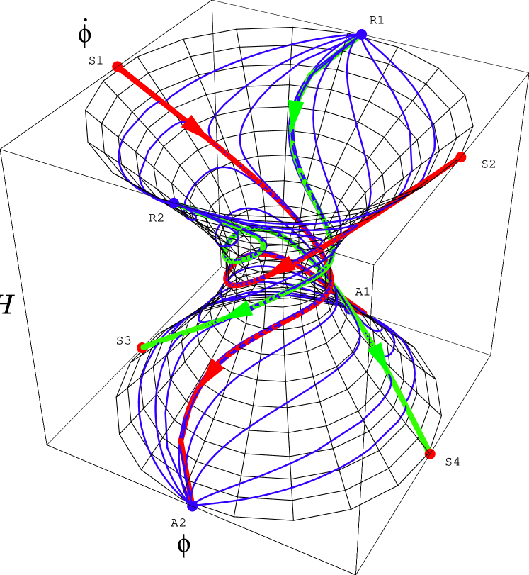
Figure 6: Phase portrait for the theory $V(\phi)={1\over 2}m^{2}\phi^{2}+V_{0}$ for $V_{0}<0$. The branches describing stages of expansion and contraction (upper and lower parts of the hyperboloid) are connected by a throat.

To show a 2d projection of the flat universe hypersurface for this model, we have to plot both the expanding and contracting branches, as depicted on Figure 7. Trajectories in the expanding universe region spiral in towards the center. When they touch the inner circle, the “throat” of the hyperboloid, they pass into the contracting universe region. There they spiral back out to infinity, i.e. the big crunch. Thus typical trajectories in this scenario pass through the three regimes described above, kinetic energy domination, potential energy domination, and oscillations, and then pass back through them in reverse order. As before, including particle production will typically introduce a matter/radiation dominated regime after the first stage of oscillations. Eventually, however, the matter and radiation will redshift away and the universe will begin contracting. We will examine this process in more detail in the next section.

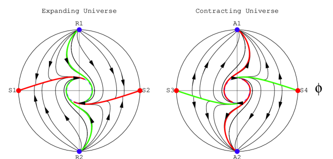
Figure 7: Left: $(\phi,\dot{\phi})$ projection of the $H>0$ branch. Right: $(\phi,\dot{\phi})$ projection of the $H<0$ branch. Trajectories from the left panel continue on the right panel.

Aside from this “wormhole” connecting the expanding and contracting branches this phase portrait looks a lot like the one for $V_{0}>0$ shown in Figure 4. Note, however, that in this case the separatrices emanating from the saddle points $S_{1}$ and $S_{2}$ no longer spiral in to the center, but rather end up reaching the points $A_{1}$ and $A_{2}$. Likewise there are separatrices that begin at $R_{1}$ and $R_{2}$ and end on $S_{3}$ and $S_{4}$. In the expanding phase their segments and segments of nearby trajectories represent the rare cases that manage to avoid inflation. In the contracting phase they become the marginal trajectories separating those that end at positive and negative $\phi$. The number of windings (i.e. field oscillations) can be estimated by setting $m^{2}\phi^{2}/2=|V_{0}|$ and using (36) to give

$$N\approx{{m}\over{6\sqrt{|V_{0}|}}}\ .$$ (38)

(This number of windings can be used to determine which repulsors and attractors are connected to which saddle points, e.g. whether the separatrix that begins at $R_{1}$ ends at $S_{3}$ or $S_{4}$.)

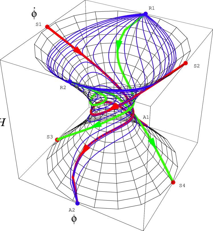
Figure 8: A different version of the phase portrait for the theory $V(\phi)={1\over 2}m^{2}\phi^{2}+V_{0}$ for $V_{0}<0$. We begin with the trajectories evenly distributed with respect to the initial values of $\phi$ in the early universe (upper part of the hyperboloid) and see what happens to them in the lower part. These trajectories are concentrated near the red separatrices and repulsed from the green ones.

The phase portraits shown above were constructed in a way symmetric with respect to time reversal, $t\to-t$. This is a legitimate approach, since our equations allow all of the solutions shown in the previous figures. However, one can obtain some additional information if, for example, one considers trajectories equally distributed with respect to the initial value of the field $\phi$ at the Planck time and follows their evolution from the region with $H>0$ to the region with $H<0$.

If we do so, the phase portrait shown in Fig. 6 starts looking somewhat different. Almost no trajectories beginning in the upper part of the hyperboloid are seen in its lower part, and those few that can be seen there are positioned very close to the (red) separatrices going from $S1$ to $A2$, and from $S2$ to $A1$ see Fig. 8. No trajectories are seen near the (green) lines going from $R1$ to $S3$ and from $R2$ to $S4$. This might seem surprising because these lines are solutions of the equations of motion, so there must be other solutions nearby. Indeed we have seen them in Fig. 7. However, the (red) lines going from $S1$ to $A2$ and from $S2$ to $A1$ are strong attractors in the regime $H<0$, whereas the lines going from $R1$ to $S3$ and from $R2$ to $S4$ are strong repulsors. Therefore most of the trajectories originating at $H>0$ and homogeneously distributed with respect to the field $\phi$ at the Planck density are repelled from the lines going from $R1$ to $S3$ and from $R2$ to $S4$, and tend to merge with the lines going from $S1$ to $A2$ and from $S2$ to $A1$.

This effect is especially apparent in the 2d phase portrait, where we do not make the Poincaré mapping, see Fig. 9. Most of the trajectories coming from the panel with $H>0$ have merged with the red separatrix on the panel corresponding to $H<0$.

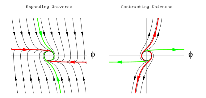
Figure 9: As in the previous figure, we begin with the trajectories evenly distributed with respect to the initial values of $\phi$ in the early universe. However, now we show a 2d projection of these trajectories, without Poincaré mapping. Left: $(\phi,\dot{\phi})$ projection of the $H>0$ branch. Right: $(\phi,\dot{\phi})$ projection of the $H<0$ branch. Trajectories from the left panel continue on the right panel.

An important (and obvious) feature of the 3d phase portraits Fig. 6 and Fig. 8 is that the separatrices, as well as other trajectories, never intersect in 3d. This is a trivial consequence of the fact that we are solving a system of 3 first order equations for 3 variables, $\phi$, $\dot{\phi}$ and $H$. One of implications of this fact is that a bunch of trajectories in the immediate vicinity of the (green) lines going from $R1$ to $S3$ and from $R2$ to $S4$ never reach the inflationary regime described by the (red) inflationary separatrices going from $S1$ to $A2$ and from $S2$ to $A1$. Only the trajectories that are sufficiently far away from the green lines going from $R1$ to $S3$ and from $R2$ to $S4$ can enter the stage of inflation.

This observation will be important for us when we describe the cyclic scenario [10], see Section 9. In this regime the red inflationary separatrices reach the singularity and are supposed to bounce back. In the language of the phase portraits this bouncing back implies that the end of the red line going from $S1$ to $A2$ becomes the beginning of the green line going from $R1$ to $S3$. But in this case the universe cannot attain the inflationary regime, since the trajectories close to the green line never switch to the vicinity of the red line. Thus the cyclic regime is possible only if bouncing from the singularity shifts the trajectory to the right from the green separatrix. From Fig. 9 it is obvious that this shift may happen either due to an increase of $\dot{\phi}$ or due to an increase of the field $\phi$.

The evolution of this system in an open or closed universe is not very different from the flat universe evolution, although the phase space is three dimensional. Because of the structure of the trajectory flow between their ends at the infinite critical points, all trajectories pass from expansion to contraction, even for an open universe. As with $V_{0}>0$ the trajectories for the open and closed cases will tend to asymptotically approach the flat universe hypersurface, and more specifically will tend to approach the inflationary separatrices. As before, however, the closed universe will include some trajectories that quickly collapse before experiencing inflation.

It is instructive to estimate the time that the universe may spend in its post-inflationary expanding phase before it begins to contract. The energy density of the oscillations of the scalar field, just like the energy density of nonrelativistic matter, decreases as $\rho_{\rm CDM}\sim{4\over 3t^{2}}$. The universe begins to collapse at $\rho_{\rm CDM}+V_{0}=0$. This happens at $t\sim{2\over\sqrt{3|V_{0}|}}$. As one could expect, this time can be greater than the present age of the universe only if $|V_{0}|\mathrel{\hbox{\hbox to0.0pt{\hbox{\lower 4.0pt\hbox{$\sim$}}\hss}\hbox{$<$}}}10^{-120}$.

This estimate remains true for a wide variety of potentials and for matter with any reasonable equation of state. However, in the theories where $V(\phi)$ has a very flat plateau or a local minimum, the universe may spend a very long time before the field $\phi$ falls down to the minimum with $V(\phi)<0$ [7, 8, 10]. Therefore in general the life-time of the universe may be very large even in theories with a very deep minimum of $V(\phi)$.

6 Going from expansion to contraction in the model $V(\phi)={m^{2}\over 2}\phi^{2}+V_{0}$

Having analysed general properties of phase portraits in the theory $V(\phi)={m^{2}\over 2}\phi^{2}+V_{0}$, let us study in a more detailed way the most interesting feature of the models with $V_{0}<0$, the switch from expansion to contraction. It is always possible to study this process numerically, but sometimes one can do better than that.

It will be convenient to represent $V(\phi)={m^{2}\over 2}\phi^{2}+V_{0}$ in the form

$$V(\phi)={m^{2}\over 2}(\phi^{2}-\phi_{0}^{2})\ .$$ (39)

This potential has a minimum at $\phi=0$, where it takes a negative value $V(\phi)=-{m^{2}\over 2}\phi_{0}^{2}$. The potential vanishes ($V(\phi)=0$) at $\phi=\pm\phi_{0}$.

Let us assume, in the first approximation, that the scale factor of the universe does not change much during each oscillation of the field $\phi$. In such a case the field $\phi$ would experience a simple oscillatory motion,

$$\phi(t)=\Phi~{}\cos mt\ ,$$ (40)

where $\Phi$ is the amplitude of the oscillations. In this case the total energy density of the scalar field would remain constant, $\rho={m^{2}\over 2}(\Phi^{2}-\phi_{0}^{2})$.

This approximation works well for $\Phi\approx\phi_{0}$. For $\Phi>\phi_{0}$, there are two cosmological solutions, describing either an expanding universe with $H=+m\sqrt{(\Phi^{2}-\phi_{0}^{2})/6}$ or a contracting universe with $H=-m\sqrt{(\Phi^{2}-\phi_{0}^{2})/6}$.

If the Hubble constant $H$ is positive, the amplitude of the field and its total energy density decrease. If the initial amplitude of the oscillations is much greater than $\phi_{0}$, the field oscillates with a slowly decreasing amplitude until it approaches $\phi_{0}$. But the energy density cannot decrease too much because at the moment when $\rho=V(\phi)+\dot{\phi}^{2}/2$ vanishes, the Hubble constant vanishes too, so that $\dot{a}=0$. Then the universe begins to collapse, $\dot{a}<0$, and the amplitude of the oscillations begins to grow. Eventually this growth becomes so fast that the field stops oscillating and moves towards $\phi=\pm\infty$.

The best way to understand this effect is to examine what happens during the critical oscillation when the sign of $\dot{a}$ changes. We will study this process analytically, making some simplifying approximations.

First of all, we will assume that the field $\phi$ begins this oscillation at $t=0$ moving with zero initial velocity from a point $\phi_{1}\approx\phi_{0}$ such that $0<\Delta\phi=\phi_{1}-\phi_{0}\ll\phi_{0}$. The initial energy density of the field is $\Delta V=V(\phi_{1})={m^{2}\over 2}(\phi_{1}^{2}-\phi_{0}^{2})\ll|V(0)|$. We will try to evaluate the turning point moment $t_{c}$ where $\dot{a}=0$ (i.e. $H=0$).

Let us consider the series expansion of the Hubble parameter around the beginning of this process

$$H(t)\approx H_{1}+\dot{H}_{1}t+{1\over 2}\ddot{H}_{1}t^{2}+{1\over 3!}\,{}^{{}^{{}^{\bf\centerdot\centerdot\centerdot}}}\hskip-10.52737ptH_{1}t^{3}+...\ ,$$ (41)

where $H_{1}$ and its derivatives are taken at $t=0$. The reason to include the terms up to $t^{3}$ in this series is the following. From the relation $\dot{H}=-{1\over 2}\dot{\phi}^{2}$ we find that for vanishing initial velocity $\dot{\phi}_{1}=0$ one has $\dot{H}_{1}=\ddot{H}_{1}=0$. The first nonvanishing coefficient ${}^{{}^{{}^{\bf\centerdot\centerdot\centerdot}}}\hskip-10.52737ptH_{1}\approx-\ddot{\phi}^{2}\approx-(V^{\prime}(\phi_{1}))^{2}=-m^{4}\phi_{1}^{2}$ is negative. Note that $H_{1}=\sqrt{V(\phi_{1})/3}=\sqrt{\Delta V/3}$. This means that at the moment

$$t_{c}\approx\left({12\,V(\phi_{1})\over(V^{\prime}(\phi_{1}))^{4}}\right)^{1/6}=m^{-1}\left({12\,\Delta V\over m^{2}\phi_{0}^{4}}\right)^{1/6}$$ (42)

the Hubble parameter vanishes. Note that the first part of this equation is pretty general, whereas the second one is specific to quadratic potentials.

At the turning point

$$\phi_{c}\approx\phi_{0}-\left({3\Delta V\over 2m^{2}\phi_{0}}\right)^{1/3}\ .$$ (43)

These results imply that the turn occurs during the first oscillation starting at $\phi_{1}$ if $\Delta V\mathrel{\hbox{\hbox to0.0pt{\hbox{\lower 4.0pt\hbox{$\sim$}}\hss}\hbox{$<$}}}m^{2}\phi_{0}^{4}$, i.e. $\phi_{1}^{2}-\phi_{0}^{2}\mathrel{\hbox{\hbox to0.0pt{\hbox{\lower 4.0pt\hbox{$\sim$}}\hss}\hbox{$<$}}}\phi_{0}^{4}$. In the most interesting case $\Delta V\ll m^{2}\phi_{0}^{4}$ the turn occurs in the immediate vicinity of the point $\phi_{0}$ where the potential becomes negative.

To study the subsequent evolution of $\phi(t)$ and $a(t)$, let us assume that the scale factor $a$ during the first oscillation does not change much. This is a reasonable assumption since $\dot{a}=0$ at the turning point. We will therefore take $a=1$ during this oscillation, and $\phi(t)=\phi_{1}~{}\cos mt$. The potential energy density of the field is

$$V(\phi)=\Delta V-{m^{2}\phi_{1}^{2}\over 2}~{}\sin^{2}mt\$$ (44)

and the acceleration of the universe is given by

$$\ddot{a}\approx{\ddot{a}\over a}={V-\dot{\phi}^{2}\over 3}={\Delta V\over 3}-{m^{2}\phi_{1}^{2}\over 2}~{}\sin^{2}mt\ .$$ (45)

Taking into account that initially $\dot{a}=a\sqrt{\Delta V/3}\approx\sqrt{\Delta V/3}$, this yields

$$\dot{a}\approx{\Delta V\over 3}t-{m^{2}\phi_{1}^{2}\over 4}t+{m\phi_{1}^{2}\over 8}~{}\sin 2mt+\sqrt{\Delta V/3}\ .$$ (46)

By integrating this relation from $t=0$ to $t=\pi/m$, i.e. during one half of an oscillation, one finds that the condition $a\approx 1$ implies then that $\phi_{1}\approx\phi_{0}\ll 1$, i.e $\phi_{0}\ll M_{p}$.

Now we are going to find how the energy density $\rho$ of the field $\phi$ changes during the time $\pi/m$ when the field $\phi$ moves from $\phi_{1}$ to $-\phi_{1}$. In order to do it, we will represent the scalar field equation $\ddot{\phi}+3H\dot{\phi}=-V^{\prime}(\phi)$ in the form

$$\dot{\rho}={d(V+\dot{\phi}^{2}/2)\over dt}=-3H\dot{\phi}^{2}\ .$$ (47)

Thus in order to find the total change of the energy density of the scalar field during some time one should integrate $-3H\dot{\phi}^{2}$:

$$\Delta\rho=\Delta(V+\dot{\phi}^{2}/2)=-3\int\limits_{t_{0}}^{t}H\dot{\phi}^{2}dt\ .$$ (48)

Using this equation, one can find the change of the energy density of the field $\phi$ during the time $\pi/m$ when the field $\phi$ moves from $\phi_{1}$ to $-\phi_{1}$:

$$\Delta\rho_{-}={3\pi^{2}\over 16}m^{2}\phi_{1}^{4}-{\pi\sqrt{3\Delta V}\over 2}m\phi_{1}^{2}-{\pi^{2}\over 4}\Delta V\phi_{1}^{2}\ .$$ (49)

In the most interesting case $\phi_{1}\approx\phi_{0}$, one can neglect the last term in this equation and replace $\phi_{1}$ by $\phi_{0}$:

$$\Delta\rho_{-}={3\pi^{2}\over 16}m^{2}\phi_{0}^{4}-{\pi\sqrt{3\Delta V}\over 2}m\phi_{0}^{2}\ .$$ (50)

Thus, if the initial kinetic energy of the field is equal to zero at the beginning of the oscillation at $\phi=\phi_{1}$, at the moment when the field $\phi$ will reach the point $-\phi_{1}$ its kinetic energy will be positive,

$${\dot{\phi}^{2}\over 2}=\Delta\rho_{-}={3\pi^{2}\over 16}m^{2}\phi_{0}^{4}-{\pi\sqrt{3\Delta V}\over 2}m\phi_{0}^{2}\ .$$ (51)

Note that for $\Delta V\ll m^{2}\phi_{0}^{4}$ the last term is much smaller than the first one, so one finds, in the first approximation, that the field $\phi$ coming to the point $-\phi_{1}$ acquires kinetic energy

$${\dot{\phi}^{2}\over 2}=\Delta\rho_{-}\approx{3\pi^{2}\over 16}m^{2}\phi_{0}^{4}={3\pi^{2}\phi_{0}^{2}\over 8}~{}V_{0}\ll V_{0}\ ,$$ (52)

and velocity

$$\dot{\phi}\approx\sqrt{3\pi^{2}\over 8}m\phi_{0}^{2}\ .$$ (53)

This velocity continues to grow during subsequent oscillations and eventually the scalar field $\phi$ and the scale factor $a$ blow up, as shown in Fig. 2.

So far we have studied an expanding universe that stops its expansion and collapses. But what if it was collapsing at the beginning of the oscillation? Suppose the scalar field was moving very slowly until it reached the point $\phi_{1}$. Then it started falling down, just as in the case considered above. However, this time we will assume that the universe was not expanding but collapsing. This corresponds to the choice $\dot{a}=-\sqrt{\Delta V/3}$ at the beginning of the process.

In this case the universe will continue collapsing with ever growing speed. The evolution of the field $\phi$ can be studied by the same methods as the ones used above. The main difference will be that the field $\phi$ passing through the point $\phi=-\phi_{1}\approx\phi_{0}$ will have kinetic energy

$${\dot{\phi}^{2}\over 2}=\Delta\rho_{+}={3\pi^{2}\over 16}m^{2}\phi_{0}^{4}+{\pi\sqrt{3\Delta V}\over 2}m\phi_{0}^{2}\ .$$ (54)

The kinetic energy of the field $\phi$ at $\phi=-\phi_{0}$ differs from that at $\phi=-\phi_{1}$ by $\Delta V$. However, for $\Delta V\ll m^{2}\phi_{0}^{4}$ this difference is much smaller than each of the terms in Eqs. (50), (54). Thus these two equations with the above-mentioned accuracy give the kinetic energy of the field $\phi$ not only at $\phi=-\phi_{1}$ but also at $\phi=-\phi_{0}$.

This discussion, as well as the difference between $\Delta\rho_{-}$ and $\Delta\rho_{+}$, will play an important role in our investigation of the cyclic universe scenario [10]. As we will see, the cyclic regime is possible only if the field $\phi$, after bouncing from the singularity, approaches the point $-\phi_{0}$ with energy density greater than $\Delta\rho_{+}$, which in its turn is greater than $\Delta\rho_{-}$, which is the energy of this field at the point $-\phi_{0}$ on its way towards the singularity. Thus one needs this field to bounce from the singularity with an increased energy, and one should check that the possible source of this additional energy does not create problems for the scenario. In fact, we will see that with an account taken of particle production, the required energy increase can be much greater than the difference between $\Delta\rho_{+}$ and $\Delta\rho_{-}$.

7 Other models with $V(\phi)<0$

Until now we have studied only one simple model with a quadratic potential. However, many features of models with negative potentials are model-independent. Consider, for example, the model with the “inverted potential” $V(\phi)=V_{0}-{m^{2}\phi^{2}\over 2}$ with $V_{0}>0$. This is the simplest example of a potential unbounded from below. The evolution of the scalar field and scale factor in this model is shown in Fig. 10. As we see, in the beginning the universe experiences a stage of inflation when the scalar field slowly rolls from the top of the effective potential. (We considered a model with $V_{0}\gg m^{2}$.) Later on, inflation ends and the speed of the field increases. If one neglects the effects of the expansion of the universe, at large $\phi$ one has $\dot{\phi}^{2}=2(V_{0}-V(\phi))$. Therefore

$${\ddot{a}\over a}={1\over 3}(V(\phi)-\dot{\phi}^{2})=V(\phi)-{2\over 3}V_{0}\ .$$ (55)

At large $\phi$ the universe starts moving with ever growing negative acceleration. If one takes into account the expansion of the universe, $\dot{\phi}^{2}$ becomes even smaller, and the deceleration is even greater. As a result, the expansion slows down and the universe starts contracting. At this stage the “friction term” $3H\dot{\phi}$ in the equation of motion of the scalar field becomes negative, which causes the field $\phi$ to grow and leads to a rapid collapse of the universe.

Figure 10: Evolution of the scalar field and scale factor in the model $V(\phi)=V_{0}-{m^{2}\phi^{2}\over 2}$.

Another example is the standard potential used for the description of spontaneous symmetry breaking, with the addition of a negative cosmological constant $V_{0}<0$:

$$V(\phi)={\lambda\over 4}(\phi^{2}-v^{2})^{2}+V_{0}=-{1\over 2}m^{2}\phi^{2}+{m^{2}\over 4v^{2}}\phi^{4}+{1\over 4}m^{2}v^{2}+V_{0}\ .$$ (56)

Here $m^{2}\equiv\lambda v^{2}$ and the point $\phi=v$ corresponds to the minimum of $V(\phi)$ with symmetry breaking. The potential $V(\phi)$ becomes equal to $V_{0}<0$ in the minimum of $V(\phi)$ at $\phi=v$. As we see in Fig. 11, the scalar field in this case experiences a stage of oscillations near the minimum of the effective potential with $V(\phi)=V_{0}<0$, but then it jumps off the minimum and blows up because of the “negative friction” in the collapsing universe. For most model parameters and initial conditions, if the field originally moves towards the minimum with $\phi=+v$ it will blow up in the direction $\phi\to-\infty$ and vice versa. The reason is that at the initial stages of the development of the instability the field $\phi$ is most efficiently accelerated by the negative friction if for a while it moves in a relatively flat direction, i.e. from one minimum to another, instead of directly moving upwards [8].

Figure 11: Evolution of the scalar field and the scale factor in the model $V(\phi)={\lambda\over 4}(\phi^{2}-v^{2})^{2}+V_{0}$, with $V_{0}<0$.

When the field accelerates enough it enters the regime $\dot{\phi}^{2}\gg V(\phi)$ and continues growing with a speed practically independent of $V(\phi)$: $\phi\sim\ln t$, $\dot{\phi}\sim t^{-1}$, see Eq. (18). So for all potentials $V(\phi)$ growing at large $\phi$ no faster than some power of $\phi$ one has $\dot{\phi}^{2}/2$ growing much faster than $V(\phi)$ (a power law singularity versus a logarithmic singularity). This means that one can indeed neglect $V(\phi)$ in the investigation of the singularity, virtually independently of the choice of the potential. Thus we see that from the point of view of the singular behavior of the field $\phi(t)$ and the scale factor, potentials having a global minimum with $V(\phi)<0$ are as dangerous as potentials unbounded from below.

Since a small modification of the potential (shifting the minimum of $V(\phi)$ towards $V(\phi)<0$) may lead to a change of regime from expansion to contraction, one may wonder whether some other modification of $V(\phi)$ can switch the regime of contraction back to expansion? The answer follows from the equation $\dot{H}=-\frac{1}{2}(\rho+p)$. This equation implies that $\dot{H}\leq 0$ because $\rho+p\geq 0$ in accordance with the null energy condition. This means, in particular, that if the universe switches from expansion to contraction, it cannot later return to the regime of expansion. The only possible exception would be if the universe were to pass through a stage of super-Planckian density in which the Einstein equations were invalid.

Even though many properties of the theories with negative potentials are model-independent, the topology of their phase portraits depends on the choice of the potential $V(\phi)$. For example, the hypersurface representing a flat universe in the theory $V(\phi)=V_{0}-{m^{2}\phi^{2}\over 2}$ is given by the constraint equation

$$\dot{\phi}^{2}=6H^{2}+m^{2}\phi^{2}-2V_{0}\ .$$ (57)

This equation describes a hyperboloid just like the flat universe hypersurface of the theory $V(\phi)=V_{0}+{m^{2}\phi^{2}\over 2}$. In this case, however, the axis of the hyperboloid is in the $\dot{\phi}$ direction rather than the $H$ direction. Moreover, the hyperboloid for this model has two sheets for $V_{0}<0$ and one sheet for $V_{0}>0$, which is the reverse of the situation for $V(\phi)=V_{0}+{m^{2}\phi^{2}\over 2}$. The different orientation of the hyperboloid means, for example, that for the theory unbounded from below all trajectories end in a Big Crunch singularity, regardless of the signs of $V_{0}$ and $k$.

8 Approach to the Singularity, Quantum Corrections, and Particle Production

Talking about the dynamics of the cosmological scalar field, until now we have remained in the realm of classical physics. We ignored possible quantum effects, and in particular the effects of particle production. These effects may lead to some important qualitative changes of the phase portraits, however, especially near the singularity.

First of all, near the singularity one may need to take into account quantum corrections to the effective action of general relativity. Even ignoring possible effects related to brane cosmology or M-theory, one may need to add to the effective action terms proportional to $R^{2}$, $R_{\mu\nu}R^{\mu\nu}$, etc.

An important example of such a theory is given by a combination of scalar field theory and the Starobinsky model, where the effective Lagrangian has additional terms $\sim R^{2}$ [24]. Whereas this addition is not very significant at low energies, it completely changes the behavior of the theory near the singularity.

For example, in the absence of this term the generic regime for a scalar field approaching the singularity is $\dot{\phi}^{2}/2\gg V(\phi)$, which corresponds to the equation of state $p=\rho$. This regime was recently discussed in [29] in the context of string cosmology. As we have seen, in this case $a\sim t^{1/3}$, $\phi\sim\ln t$.

However, if one adds the term $R^{2}$, the most general regime for theories where the potential is not too steep becomes quite different: $a\sim t^{1/2}$, $\phi\sim t^{-1/2}$ [24].

It is even more important to consider the effects of particle production. If one ignores quantum effects, one typically finds the curvature $R\sim t^{-2}$ in a collapsing universe. Scalar particles minimally coupled to gravity, as well as gravitons and helicity 1/2 gravitinos [30], are not conformally invariant; their frequencies thus experience rapid nonadiabatic changes induced by the changing curvature. These changes lead to particle production due to nonadiabaticity with typical momenta $k^{2}\sim R\sim t^{-2}$. The total energy-momentum tensor of such particles produced at a time $t$ after (or before) the singularity is $T_{\mu\nu}\sim O(k^{4})\sim R^{2}\sim t^{-4}$ [31, 32]. Comparing the density of produced particles with the classical matter or radiation density of the universe $\rho\sim t^{-2}$, one finds that the density of created particles produced at the Planck time $t\sim 1$ is of the same order as the total energy density in the universe.

The main point of this discussion is that particle production near a cosmological singularity can be extremely efficient. Generically one expects that when the universe emerges from or approaches a singularity and its density is close to the Planck density, the density of produced particles should be comparable to the total energy density of the universe.

This is a pretty general conclusion. For example, in brane cosmology a similar effect of particle production may occur even though $R=0$ in 4D. Indeed, the change of distance between branes leads to a nonadiabatic change of the spectrum of Kaluza-Klein modes and thus to particle production; one may call it a time-dependent Casimir effect. Note that this effect exists even in theories with unbroken supersymmetry [33].

This observation has many implications. In particular, one can no longer expect that matter (or a scalar field) has the equation of state $p=\rho$ near the singularity. Even if the universe around the Planck time was dominated by matter with $p=\rho$, the creation of particles would immediately change the situation. And even if the density of created particles initially was somewhat smaller than the energy density of matter with $p=\rho$, this situation would rapidly change. The density of the component of matter with $p=\rho$ decreases as $a^{-6}$, whereas the energy density of radiation and nonrelativistic particles decrease as $a^{-4}$ and $a^{-3}$ respectively. Therefore the energy density of such particles soon becomes greater than the energy density of the matter component with $p=\rho$. Once this happens the scalar field immediately freezes. It loses its initial kinetic energy and begins moving very slowly. As we already discussed, this provides perfect initial conditions for inflation. This result also has important implications for the cyclic universe scenario [10].

9 Cyclic universe

9.1 The basic scenario

Until now we have studied the evolution of the universe and classified new possibilities that appear in scalar theories with negative potentials. This problem is very interesting. Its investigation has already brought us to an important realization: We cannot live in anti de Sitter space dominated by a negative cosmological constant, not because the negative cosmological constant is forbidden, but because a universe dominated by negative vacuum energy cannot appear after a long stage of inflation [6, 7, 8]. Another interesting realization is that the available observational data can tell us nothing about the future of the universe: we may live in a stage of a nearly constant de Sitter-like inflationary acceleration, but it may end with a global collapse [34, 35, 36, 7, 8].

A common feature of cosmological evolution in models with negative potentials is that it begins in a singularity and ends in a singularity, even if the universe is not closed. This was not the case for the theories with $V(\phi)>0$, where the universe may continue expanding forever and never end in a singularity even if it is closed.

This naturally brought back old speculations about the oscillating, or cyclic, evolution of the universe, see e.g. [16] - [22], [10]. The universe may be created in a singularity, then collapse and re-emerge again.

There is a certain intellectual attractiveness in this idea. However, during the last 20 years this idea has lost some of its initial appeal. Indeed, if there was a stage of inflation after the singularity, then the initial conditions producing our universe are nearly irrelevant for the investigation of the formation of large-scale structure in the observable part of the universe. Moreover, inflation in many of its simplest versions is eternal [37, 38]. This fact may not solve the singularity problem [39], but it puts the origin of our part of the universe indefinitely far away in the past [40].

Recently Steinhardt and Turok proposed a version of inflationary theory where the stage of inflation occurs after formation of the large scale structure of the universe and perturbations responsible for the formation of the structure of the universe are produced before the singularity, during the previous cycle of the universe evolution [10]. In this scenario inflation does not protect us from all uncertainties associated with the physical processes occurring around the big bang. On the contrary, in order to describe our universe in this scenario one must know exactly what happens with small perturbations of the metric when they pass through the singularity.

The cyclic scenario [10] is a modified version of the ekpyrotic scenario [11]. It is based on the idea that we live on one of two branes whose separation can be parametrized by a scalar field $\phi$. It is assumed that one can describe the brane interaction by an effective 4D theory with the effective potential $V(\phi)$ having a minimum at $V(\phi)<0$. In the original version of the ekpyrotic scenario it was assumed that $V(\phi)$ is always negative, but it vanishes at $\phi=0$ and at $\phi\to\infty$. It was claimed that one of the main advantages of the ekpyrotic scenario was the absence of a cosmological singularity and the possibility to solve the major cosmological problems without the help of inflation, which was called “superluminal expansion.”

However, later it was found that it is difficult to solve the cosmological problems in the ekpyrotic scenario without using inflation [12]. Moreover, perturbations of the field $\phi$ that could be responsible for large scale structure formation in this scenario are generated due to tachyonic instability [41] at the time when $V(\phi)$ was supposed to be smaller than $-10^{-50}$ in Planck units. Therefore it is difficult to avoid inflation in this model: Even a miniscule positive contribution to $V(\phi)$ of the order $10^{-50}$ would lead to a stage of exponential expansion of the universe at large $\phi$ [12]. Also, in [42] it was shown that in the context of the effective 4D theory used in [11] the universe can only collapse. This means that the ekpyrotic scenario suffers from the cosmological singularity problem. This problem has been analysed in [13], but so far it remains unresolved.

In the cyclic universe scenario the authors assume, in accordance with the suggestion of Ref. [12], that $V(\phi)$ is positive at large $\phi$, and therefore the universe experiences a stage of inflation. This stage provides the solution to the major cosmological problems. However, it is assumed that this is an extremely low-scale inflation associated with the present stage of acceleration of the universe in a state with $V(\phi)\sim 10^{-120}$. Inflationary perturbations produced at this stage have wavelengths comparable to the present size of the horizon, so they cannot be responsible for galaxy formation.

Figure 12: Scalar field potential in the cyclic scenario. The minimum of the potential may occur at any value of $\phi$; in this section for simplicity we will assume that it occurs at $\phi=0$; we will consider a more general situation later.

Therefore it is assumed that the desired perturbations of the scalar field are produced after inflation, by the same tachyonic mechanism as in the ekpyrotic scenario [41, 11, 12]. The effective potential of the scalar field in the cyclic scenario has the shape shown in Fig. 12. Inflation occurs at large $\phi$. Once the field rolls down to the region where $V(\phi)<0$, the universe begins to collapse. At that time perturbations of the scalar field are generated. The speed of the field in a collapsing universe grows. It reaches the plateau at $\phi\to-\infty$ where, according to [10], the potential vanishes. The universe enters the regime where its energy density is dominated by the kinetic energy of the scalar field, and it evolves towards the singularity in accordance with Eqs. (17), (18).

Usually, this would be considered the end of the evolution of the universe. However, in the cyclic scenario it is assumed that the universe goes through the singularity and re-appears again. When it appears, in the first approximation it looks exactly as it was before, and the scalar field moves back exactly by the same trajectory by which it reached the singularity [13].

This is not a desirable cyclic regime. Therefore it is assumed in [10] that the value of kinetic energy of the field $\phi$ increases after the bounce from the singularity. This increase is supposed to appear as a result of particle production at the moment of the brane collision (even though one could argue that usually particle production leads to an opposite effect). If the increase of the kinetic energy is large enough, the field $\phi$ rapidly rolls over the minimum of $V(\phi)$ in a state with a positive total energy density, and continues its motion at $\phi>0$. The kinetic energy of the field decreases faster than the energy of matter produced at the singularity. At some moment the energy of matter begins to dominate. Eventually (a few billion years after the big bang) galaxies form. Then the energy density of ordinary matter becomes smaller than $V(\phi)$ and the present stage of inflation (acceleration of the universe) starts again.

As we see, this version of the ekpyrotic scenario is not an alternative to inflation anymore. Rather it is a very specific version of inflationary theory. The major cosmological problems are supposed to be solved due to exponential expansion in a vacuum-like state, even though the mechanism of production of density perturbations in this scenario is non-standard. Let us remember that Guth’s first paper on inflation [2] was greeted with so much enthusiasm precisely because it proposed a solution to the homogeneity, isotropy, flatness and horizon problems, even though it didn’t address the formation of large scale structure. The Starobinsky model that was proposed a year earlier [1] could account for large scale structure and the observed CMB anisotropy [43], but it did not attract as much attention because it did not emphasize the possibility of solving these initial condition problems.

In fact, the stage of acceleration of the universe in the cyclic model is eternal inflation. Indeed, the main criterion for the process of self-reproduction of the inflationary universe to occur is that the amplitude of inflationary perturbations $\delta\phi\sim H\sim\sqrt{V}$ should be greater than the change $\Delta\phi$ of the classical value of the field $\phi$ during the time $H^{-1}$:  $\Delta\phi\sim V^{\prime}/V$ [37, 38, 40]. For the potential $V(\phi)$ used in the cyclic model one has $\delta\phi=const$ in the limit $\phi\to\infty$, whereas $\Delta\phi\to 0$ in this limit. Thus the universe at large $\phi$ enters the stage of eternal self-reproduction, quite independently of the possibility to go through the singularity and re-appear again. In other words, the universe in the cyclic scenario is not just a chain of eternal repetition, but a growing self-reproducing inflationary fractal of the type discussed in [37, 38, 40].

One may wonder, however, whether this version of inflationary theory is good enough to solve all major cosmological problems. Indeed, inflation in this scenario may occur only at a density 120 orders of magnitude smaller than the Planck density. If, for example, one considers a closed universe filled with matter and a scalar field with the potential used in the cyclic model, it will typically collapse within the Planck time $t\sim 1$, so it will not survive until the beginning of inflation in this model at $t\sim 10^{60}$. For consistency of this scenario, the overall size of the universe at the Planck time must be greater than $l\sim 10^{30}$ in Planck units, which constitutes the usual flatness problem. The total entropy of a hot universe that may survive until the beginning of inflation at $V\sim 10^{-120}$ should be greater than $10^{90}$, which is the entropy problem [25]. An estimate of the probability of quantum creation of such a universe “from nothing” gives $P\sim e^{-|S|}\sim\exp\left(-{24\pi\over V}\right)\sim e^{-120}$ [44].

There are some other unsolved problems related to this theory, such as the origin of the potential $V(\phi)$ [12] and the 5D description of the process of brane motion and collision [42, 45]. In particular, the cyclic scenario assumes that the distance between the branes is not stabilized. Thus one would need to find some other mechanism that would ensure that the effective gravitational constant, as well as other parameters depending on the field $\phi$ (i.e. on the brane separation), does not change in time too fast. This is one of the reasons why it is usually assumed that the branes in Hor̆ava-Witten theory must be stabilized.

We will not discuss these problems here. Instead of that, we will concentrate on the phenomenological description of possible cycles using the effective 4D description of this scenario. This will allow us to find out whether the cyclic regime is indeed a natural feature of the scenario proposed in [10].

For the remainder of this section we will analyse this scenario using the tools developed in the earlier sections of the paper. In Section 9.2 we will describe the phase portrait of the cyclic scenario. In Section 9.3 we will consider the conditions that must be satisfied at the bounce in order for the cyclic regime to occur. In Section 9.4 we will analyse the motion of the field as it returns from the singularity and show that the conditions described in Section 9.3 are difficult to realize self-consistently without invoking super-Planckian potentials, even in the vicinity of the minimum. Following the authors of [10] we will consider such super-Planckian potentials in Section 9.5. Aside from the problem of applying the effective 4D theory at such high energies, we will find that there are still other problems in such realizations of the scenario. In Sections 9.6 and 9.7 we will propose some modifications of the cyclic scenario that may resolve some of the problems raised here.

9.2 Phase portrait of the cyclic universe

The phase space of the cyclic scenario is the usual 3d space $(\phi,\dot{\phi},H)$. If one does not take into account matter and radiation, the phase portrait of the scenario forms a 2d surface in 3d space. It is shown in Fig. 13 without the Poincaré mapping. (If one adds radiation, the flow of trajectories becomes three dimensional.) The trajectories corresponding to different initial values of $\phi$ and $\dot{\phi}$ start at large $H$, i.e. in the upper part of Fig. 13. The trajectories beginning at large positive $\phi$ reach the (red) separatrix going from the point S1 to the point A. Its upper part ($H>0$) corresponds to inflation. These trajectories follow the separatrix towards the throat of the phase portrait at $H=0$, and then all of them move towards the singularity. The trajectories beginning at large negative $\phi$ fall from the singularity at large positive $H$ to the singularity at large negative $H$ without entering the stage of inflation.

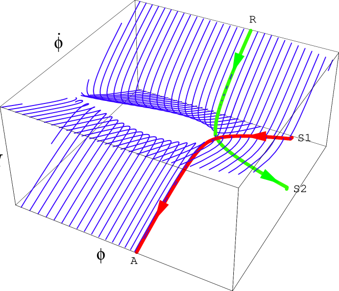
Figure 13: The 3d phase portrait for the cyclic scenario. All trajectories (blue lines) begin at $H>0$ and end in a singularity at $H<0$.

If one flips $\dot{\phi}\to-\dot{\phi}$ and $H\to-H$, which corresponds to time-reversal, the red separatrix connecting points S1 and A becomes the green separatrix connecting points R and S2. In the lower part of the figure (at negative $H$) this line corresponds to the stage of deflation (exponential contraction of the universe, which is a time-reversal of inflation). These two separatrices divide all trajectories into three topologically disconnected parts: the trajectories to the right of the green separatrix, the trajectories between the green and the red separatrix and the trajectories to the left of the red separatrix.

One could think that the green separatrix separates inflationary trajectories from the trajectories that fall to the singularity without reaching the stage of inflation. However, it is not so. As we already discussed in Section 5, the trajectories that reach the stage of inflation are at a finite distance to the right away from the green line connecting points R and S2 (i.e. at greater values of $\phi$ and $\dot{\phi}$).

The $(\phi,\dot{\phi})$ projection of the phase portrait for the cyclic scenario is shown in Fig. 14, also without the Poincaré mapping. An interesting feature of the right panel of Fig. 14 is the apparent absence of any trajectories near the green line (the right separatrix at the right panel). This might seem surprising because this line is a solution of the equations of motion, so there must be other solutions nearby. The reason is that the deflationary universe regime described by this line is a strong repulsor, just opposite to the fact that the inflationary red line at $H>0$ (the right separatrix at the left panel) is a strong attractor. As a result, the density of trajectories near the green line at $H<0$ is very small; that is why they do not show up in Fig. 14. We discussed a similar issue in Section 5.

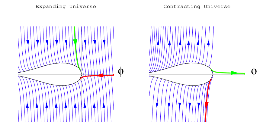
Figure 14: The 2d phase portrait for the cyclic scenario. All trajectories begin at the bounding box of the left panel ($H>0$) and end at the bounding box of the right panel ($H<0$).

As we see, all trajectories beginning at $H>0$ end up in the singularity at $H\to-\infty$. In the cyclic scenario it is assumed that the universe goes through the singularity and re-appears again. When it happens, all trajectories with $\phi<0$, $\dot{\phi}<0$ and $H<0$ the left lower part of the right panel in Fig. 14 suddenly reappear in the right upper corner of the left panel of Fig. 14, describing the trajectories starting at $\phi<0$, $\dot{\phi}>0$ and $H>0$. If one ignores particle production at the singularity, the red separatrix on the right panel becomes the green line at the left panel (time-reversal). As a result of this flip, the field $\phi$, which previously was running down along the red separatrix towards the singularity in Fig. 13, eventually returns exactly to the same place at $\phi>0$ where it was in the very beginning of the process. However, it returns back not at the stage of exponential expansion but at the stage of exponential contraction, following the green separatrix in Fig. 13.

Exponential contraction is not a desirable regime. In order to reach the cyclic inflationary regime, some of the trajectories to the left of the red separatrix after the singularity should jump sufficiently far away to the right of the green separatrix. As we already mentioned, Ref. [10] assumes that this jump may occur due to an increase in the energy of the scalar field bouncing back from the singularity. This increase in energy is supposed to happen due to particle production. Only if this jump is sufficiently large can these trajectories reach the red inflationary separatrix going from S1 to A. Then inflation begins, the field rolls to the minimum of $V(\phi)$ again, and everything repeats.

9.3 Moving towards the minimum of $V(\phi)$

To study the potential shown in Figure 12 we will assume that near the minimum it can be represented as ${m^{2}\over 2}(\phi^{2}-\phi_{0}^{2})$. At $\phi\mathrel{\hbox{\hbox to0.0pt{\hbox{\lower 4.0pt\hbox{$\sim$}}\hss}\hbox{$>$}}}\phi_{0}$ we will take it to be flat with $V\approx 10^{-120}$ and at $\phi<\phi_{0}$ we will take $V=0$. The results of a numerical investigation for more complicated potentials are very similar to the ones obtained for this simple model. However, in this model one can study everything analytically using the results obtained in Section 6. Indeed, we know how the field moves at $\phi<-\phi_{0}$, when $V(\phi)=0$, and we also know how it behaves in the quadratic potential, when it moves from $-\phi_{0}$ to $\phi_{0}$. The only thing that we need to do is to patch these two regimes together.

At the initial stage the scalar field moves extremely slowly at $\phi>\phi_{0}$ and the universe inflates. Once it reaches $\phi\approx\phi_{0}$ it falls down, $V(\phi)$ becomes negative, and the universe begins to contract. To describe this process one can use the theory developed in the first part of this paper. The contraction begins at $\phi=\phi_{c}$ (42). The scalar field reaches $\phi=-\phi_{0}$ with energy $\Delta\rho_{-}$ given by Eq. (49).

Subsequently, the field $\phi$ moves towards $\phi=-\infty$ and the singularity develops in accordance with Eq. (18). To describe this motion one should take $t_{0}=1/\sqrt{3\Delta\rho_{-}}$ in (18) and replace $\phi_{0}$ by $-\phi_{0}$:

$$\phi+\phi_{0}=\sqrt{2\over 3}\ \ln{\sqrt{3\Delta\rho_{-}}\,t}\ ,\qquad{\dot{\phi}^{2}\over 2}={1\over 3t^{2}}\ .$$ (58)

In this solution $\phi=-\phi_{0}$ at $t=t_{0}$.

Let us use this equation to find the value of the field $\phi$ at the Planck time when the energy density becomes $1$ in Planck units and one can no longer study this regime within the context of general relativity. This happens at $t_{p}=1/\sqrt{3}$ in Planck units. Therefore the scale factor of the universe $a\sim t^{1/3}$ decreases by a factor $\sim(\Delta\rho_{-})^{1/6}$ from the beginning of the process at $\phi=-\phi_{0}$ until the density becomes $O(1)$. The scalar field $\phi$ at that time is given by

$$\phi_{p}=-\phi_{0}+\sqrt{1\over 6}\ \ln{\Delta\rho_{-}}\ .$$ (59)

Setting $a(t_{p})=1$ we can write our solution as

$$\phi-\phi_{p}=\sqrt{2\over 3}\ \ln{\sqrt{3}t}\ ,\qquad{\dot{\phi}^{2}\over 2}={1\over 3t^{2}}\ ,\qquad a=3^{1/6}\,t^{1/3}\ ,$$ (60)

which in turn implies

$$\dot{\phi}={\sqrt{2}\over a^{3}},\qquad\phi-\phi_{p}=\sqrt{6}\ \ln\,a\ .$$ (61)

One can also represent our results in terms of the conformal time $\tau$, where $dt=ad\tau$. In this case $t=(2\tau\,3^{-5/6})^{3/2}$, and

$$\phi-\phi_{p}=\sqrt{3\over 2}\ \ln\,{2\,\tau\over\sqrt{3}}\ .$$ (62)

The Planck time $t_{p}=1/\sqrt{3}$ corresponds to $\tau_{p}=\sqrt{3}/2$.

The cyclic scenario requires that the universe bounce back from the singularity and the field move back from $-\infty$ to $\phi_{0}$. Depending on how much kinetic energy the field has at this point three regimes are then possible:

1. ${\dot{\phi}^{2}\over 2}\leq\Delta\rho_{-}$ at $\phi=-\phi_{0}$. This is the regime that would be reached if the bounce were perfectly symmetric (in which case ${\dot{\phi}^{2}\over 2}=\Delta\rho_{-}$). The universe starts collapsing at $\phi\leq\phi_{c}$. The field overshoots the point $\phi=\phi_{0}$ and moves with ever growing speed towards $\phi=+\infty$. There is a small bunch of trajectories such that the scalar field evolves very slowly, the equation of state is $p=-\rho$, and the universe contracts exponentially. Eventually, however, the kinetic energy of the field $\phi$ dominates and the collapse becomes power-law with $p=\rho$.

   This regime is represented by the trajectories to the left of the green separatrix in the upper part of the left panel in Fig. 14.

2. $\Delta\rho_{-}<{\dot{\phi}^{2}\over 2}<\Delta\rho_{+}$ at $\phi=-\phi_{0}$. The universe starts collapsing at $\phi>\phi_{c}$. The field does not have enough energy to reach the point $\phi=\phi_{0}$, so it returns back to negative $\phi$, the field moves with ever growing speed to $\phi=-\infty$, and a singularity develops.

   This regime is represented by a small bunch of trajectories to the right of the green separatrix in the upper part of the left panel in Fig. 14.

3. ${\dot{\phi}^{2}\over 2}\mathrel{\hbox{\hbox to0.0pt{\hbox{\lower 4.0pt\hbox{$\sim$}}\hss}\hbox{$>$}}}\Delta\rho_{+}$ at $\phi=-\phi_{0}$. The universe continues expanding and the field $\phi$ becomes greater than $\phi_{0}$. It continues growing and gradually slows down. As a result, inflation begins. Then the field very slowly decreases, falls into the minimum of $V(\phi)$, the universe collapses and the field moves to $\phi=-\infty$. This is the regime required by the cyclic scenario.

   This regime is represented by trajectories starting sufficiently far from the green separatrix, to the right of it in the upper part of the left panel in Fig. 14.

The last of these regimes requires additional explanation. Let us remember how we derived the expression for $\Delta\rho_{+}$: We considered the field $\phi$ slowly rolling from $\phi=\phi_{0}$ during the stage of contraction and found that it arrived at the point $\phi=-\phi_{0}$ with kinetic energy $\Delta\rho_{+}$. If we reverse the time evolution of the universe, we will see the scalar field rolling down from $\phi=-\phi_{0}$ and arriving at the point $\phi=\phi_{0}$ with a nearly vanishing speed during the stage of expansion. If the initial kinetic energy of the field is greater than $\Delta\rho_{+}$, it reaches the point $\phi=\phi_{0}$ with a non-vanishing speed and moves further onto the plateau where the energy density of the field $\phi$ becomes constant, and inflation begins.

As we have seen in Section 6, the difference between $\Delta\rho_{+}$ and $\Delta\rho_{-}$ is extremely small:

$$\delta\rho=\Delta\rho_{+}-\Delta\rho_{-}=\pi\sqrt{3\Delta V}\,m\phi_{0}^{2}\ .$$ (63)

Here $\Delta V$ has the meaning of the height of the effective potential at $\phi>\phi_{0}$; in our case $\Delta V\sim 10^{-120}$. Thus one might expect that it pretty easy to jump from the trajectory with energy $\Delta\rho_{-}$ to the desirable trajectory with energy greater than $\Delta\rho_{+}$, as in case 3.

In reality, however, the required jump in kinetic energy becomes much larger when one takes into account quantum effects. As the field $\phi$ moves through the minimum from $-\phi_{0}$ to $\phi_{0}$ its mass changes from $0$ to $m$ and back to $0$ again, all within a time $O(m^{-1})$ (half of an oscillation), see Fig. 16. This non-adiabatic change, ${\Delta m\over\Delta t}\sim m^{2}$, will lead to the production of $\phi$-particles with energy density $O(m^{4})$ [27]. Therefore the field $\phi$ loses an amount of energy $O(m^{4})$, which makes it less likely to reach $\phi_{0}$ while the universe is still expanding. Thus in order to realize the cyclic scenario the kinetic energy density of the field $\phi$ at the point $-\phi_{0}$ must be greater than $\Delta\rho_{+}$ by $O(m^{4})$, which is much greater than $\Delta V$.

One may wonder where the field gets this boost in kinetic energy from. Usually one would expect that the field after a bounce can only lose energy due to particle production. However, in [10] it is assumed that it can actually gain energy as a result of particle production during the brane collision (i.e. in the singularity). It is not quite clear whether this can indeed happen, see e.g. [45] where it is claimed that particles can be created during the brane collision only if they have negative energy density. We are not going to discuss this issue here. Instead of that, we will follow the assumptions of [10] and check what happens to the scalar field $\phi$ if the universe after the bounce contains some matter or radiation.

9.4 A scalar field with a vanishing potential in the presence of radiation

Let us consider the motion of the field $\phi$ from $-\infty$ to $-\phi_{0}$ in the presence of radiation. The Friedmann equation describing this process can be written as follows:

$$\left({\dot{a}\over a}\right)^{2}={1\over 3}\left({\dot{\phi}_{i}^{2}\over 2}\ {a^{6}_{i}\over a^{6}}+\rho_{i}^{r}\ {a^{4}_{i}\over a^{4}}\right)\ .$$ (64)

Here $\dot{\phi}_{i}$ is the velocity of the field at some moment $t_{i}$, $a_{i}$ is the scale factor of the universe at that moment, and $\rho_{i}^{r}$ is the density of radiation at that time. This equation reflects the fact that the kinetic energy of the field decreases as $a^{-6}$ and radiation energy decreases as $a^{-4}$ during the expansion of the universe.

It is convenient to write this equation in terms of the conformal time $\tau$, where $dt=ad\tau$:

$$(a^{\prime})^{2}={A^{2}\over a^{2}}+B\ ,$$ (65)

where $a^{\prime}={da\over d\tau}=a\,\dot{a}$, $A^{2}={\dot{\phi}_{i}^{2}a^{6}_{i}/6}$ and $B={\rho_{i}^{r}a^{4}_{i}/3}$.

Taking $a(0)=0$ (at the singularity), the solution of this equation is

$$a^{2}={2A\tau}+B\tau^{2}\ .$$ (66)

For definiteness, we will normalize our solution at the time $t_{i}=t_{p}$, when $\dot{\phi}^{2}/2=1$ and $a_{i}=1$. Then $A^{2}={1/3}$, $B={\rho_{p}^{r}/3}$, and

$$a^{2}={{2\over\sqrt{3}}\tau}+{\rho_{p}^{r}\over 3}\tau^{2}\ .$$ (67)

Then, using equation $\phi^{\prime}=\dot{\phi}_{i}a_{i}^{3}/a^{2}=\sqrt{6}A/a^{2}$, one finds

$$\phi-\tilde{\phi}_{p}=\sqrt{3\over 2}\,\ln{2\tau\over\sqrt{3}(1+{\rho_{p}^{r}\over 2\sqrt{3}}\tau)}+C_{r}=\sqrt{6}\,\ln{a\over 1+{\rho_{p}^{r}\over 2\sqrt{3}}\tau}+C_{r}\ .$$ (68)

Here $\tilde{\phi}_{p}$ is the value of the scalar field at the time when $\dot{\phi}^{2}/2=1$ after the bounce. The constant of integration $C_{r}$ is supposed to vanish in the absence of radiation, i.e. for $\rho_{p}^{r}=0$. In this case $\tilde{\phi}_{p}=\phi_{p}$, and our solution (68) coincides with the solution presented in Eq. (62). This means that in the absence of radiation the field $\phi$ elastically bounces from the singularity, in accordance with [13].

One can find the constant $C_{r}$ for any given $\rho_{p}^{r}$ from the condition that $\phi=\tilde{\phi}_{p}$ at $\dot{\phi}^{2}/2=1$ and $a=1$. In particular, for $\rho_{p}^{r}\ll 1$ one has $C_{r}\approx\rho_{p}^{r}{\sqrt{3}\over 2\sqrt{2}}$.

Eq. (68) implies that at $\rho_{p}^{r}\tau>2\sqrt{3}$ the field stops moving. Therefore we will assume that $\rho_{p}^{r}\tau\ll 1$ at $\phi<-\phi_{0}$. This leads to a strong constraint on $\rho_{p}^{r}$:

$$\rho_{p}^{r}\mathrel{\hbox{\hbox to0.0pt{\hbox{\lower 4.0pt\hbox{$\sim$}}\hss}\hbox{$<$}}}(\Delta\rho_{+})^{1/3}\ .$$ (69)

If one takes, for definiteness, $\phi_{0}\sim 0.1M_{p}$, $m^{2}\phi_{0}^{2}\sim 10^{-20}$, as in the original version of the ekpyrotic scenario [11], one finds that the cyclic scenario with these parameters cannot work unless the energy density of radiation at the Planck time is less than $10^{-6}$ in Planck units. In general the density of gravitationally produced particles is $\sim H^{4}$, which is $O(1)$ at the Planck time, so it is not clear how particle production could be so strongly suppressed.

Suppose, however, that for whatever reason one can indeed have $\rho_{p}^{r}\ll(\Delta\rho_{+})^{1/3}$. In this case $\rho_{p}^{r}\tau\ll 1$ and Eq. (68) can be represented in the following form:

$$\phi-\tilde{\phi}_{p}=\sqrt{6}\,\ln a-{\rho_{p}^{r}\over\sqrt{2}}\,(\tau-{\sqrt{3}\over 2})\ .$$ (70)

With our normalization of $a$ one has

$${1\over 2}\dot{\phi}^{2}=a^{-6}\ ,$$ (71)

As we already discussed, if we want the field to move to $\phi>\phi_{0}$ during the stage of expansion of the universe, its kinetic energy $\dot{\phi}^{2}/2$ must be greater than $\Delta\rho_{+}$ at $\phi=-\phi_{0}$. If we assume that the field has sub-Planckian energy as it moves through the minimum, i.e. that $\Delta\rho_{+}\ll 1$, then

$$\tilde{\phi}_{p}>-\phi_{0}+{1\over\sqrt{6}}\,\ln\Delta\rho_{+}+{\rho_{p}^{r}\sqrt{3}\over 2\sqrt{2}}\,(\Delta\rho_{+})^{-1/3}\ .$$ (72)

Comparison with Eq. (59) gives the following condition:

$$\tilde{\phi}_{p}-\phi_{p}>{\rho_{p}^{r}\sqrt{3}\over 2\sqrt{2}}\,(\Delta\rho_{+})^{-1/3}+{1\over\sqrt{6}}\,\ln{\Delta\rho_{+}\over\Delta\rho_{-}}\ .$$ (73)

In general, it could happen that after bouncing from the singularity the field $\phi$ appears at the Planck density at $\tilde{\phi}_{p}\not=\phi_{p}$, so that $\tilde{\phi}_{p}-\phi_{p}=O(\rho_{p}^{r})$ [10]. However, our investigation shows that the cyclic scenario with $\Delta\rho_{+}\ll 1$ could work only if $\tilde{\phi}_{p}-\phi_{p}\gg\rho_{p}^{r}$.

This means that the cyclic scenario can work only if a very small amount of radiation can produce a major change in the state of the field $\phi$ at the Planck time: $\tilde{\phi}_{p}-\phi_{p}\mathrel{\hbox{\hbox to0.0pt{\hbox{\lower 4.0pt\hbox{$\sim$}}\hss}\hbox{$>$}}}\rho_{p}^{r}\,(\Delta\rho_{+})^{-1/3}$. Second, the amount of radiation at the Planck time must be very small, $\rho_{p}^{r}\mathrel{\hbox{\hbox to0.0pt{\hbox{\lower 4.0pt\hbox{$\sim$}}\hss}\hbox{$<$}}}(\Delta\rho_{+})^{1/3}$. This may be a real problem if, as we expect, quantum effects at Planckian densities create particles with density $\rho_{p}^{r}=O(1)$.

These problems are less serious in models with $\Delta\rho_{+}\geq 1$, i.e. if the field $\phi$ acquires super-Planckian energy even before it reaches the plateau at $\phi<-\phi_{0}$. Such models are suspect because the usual 4D approach based on general relativity becomes unreliable at super-Planckian densities. It appears that such models are necessary for the cyclic model, however, and in at least one of their papers the authors of [10] invoke such a model. We therefore consider such potentials here.

9.5 Super-Planckian potentials for the cyclic scenario

Let us now consider a potential proposed by the authors of the cyclic scenario [10]:

$$V(\phi)=V_{0}~{}(1-e^{-c\phi})~{}F(\phi)\ .$$ (74)

In the particular example studied in the last paper of Ref. [10] one has $F(\phi)=e^{-e^{-\gamma\phi}}$, $V_{0}=10^{-120}$, $c=10$, $\gamma\approx 1/8$. This potential is shown in Fig. 15. This potential has the same structure as the potential shown in the Fig. 12, but the scales and the position of the minimum are determined by the parameters given in [10]. At $\phi=0$ this potential vanishes. It approaches its asymptotic value $V_{0}=10^{-120}$ at $\phi\mathrel{\hbox{\hbox to0.0pt{\hbox{\lower 4.0pt\hbox{$\sim$}}\hss}\hbox{$>$}}}1$. Inflation in this scenario is possible at $\phi\mathrel{\hbox{\hbox to0.0pt{\hbox{\lower 4.0pt\hbox{$\sim$}}\hss}\hbox{$>$}}}1$. At $\phi\mathrel{\hbox{\hbox to0.0pt{\hbox{\lower 4.0pt\hbox{$\sim$}}\hss}\hbox{$>$}}}15$ one has $V^{3/2}\mathrel{\hbox{\hbox to0.0pt{\hbox{\lower 4.0pt\hbox{$\sim$}}\hss}\hbox{$>$}}}V^{\prime}$ and the universe enters the process of eternal inflation [37, 38]. The potential has a minimum at $\phi\approx-36$; the value of the potential in this minimum is $V_{\rm min}\approx-3$.

Figure 15: An example of cyclic scenario potential used in Ref. [10].

Let us try to understand the origin of the parameters $c=10$, $\gamma\approx 1/8$ used in [10]. According to [14], the amplitude of density perturbations in this scenario in the limit $c\gg 1$ can be estimated as

$${\delta\rho\over\rho}\sim 10^{-5}\sqrt{-V_{j}}~{}\xi^{4}\ ,$$ (75)

where $V_{j}$ is approximately equal to the value of the potential in its minimum $V_{\rm min}$ and $\xi$ is the efficiency with which radiation is produced at the singularity; it is assumed that $\xi\ll 1$. This suggests that in order to be consistent with observational data (${\delta\rho\over\rho}\sim 10^{-4}$) one should have $-V_{j}\gg 1$. This means one must rely on calculations using the equations of general relativity at $|V(\phi)|\gg 1$.

The authors of [14] have warned the readers that their results are very preliminary and many authors do not agree with their derivation of the amplitude of density perturbations [15]. Therefore it may happen that the correct equation for perturbations in the cyclic scenario as well as the expression for $V(\phi)$ will be quite different. Here we will simply try to understand the values of the parameters used in [10] and check the consequences of the potential they suggested.

The spectrum of density perturbations obtained in [14] is not blue, as in [11], but red, like in the pyrotechnic scenario [12] and in the simplest versions of chaotic inflation. The spectral index is $n\approx 1-4/c^{2}$. Observational data suggest that $n=0.93\pm 0.1$, which implies that $c\mathrel{\hbox{\hbox to0.0pt{\hbox{\lower 4.0pt\hbox{$\sim$}}\hss}\hbox{$>$}}}5$. If one takes $c\gg 5$, and $V_{J}>1$, one finds that the curvature of the effective potential in its minimum becomes much greater than 1.

Once one takes $V\sim-3$ in the minimum of the potential with $c=10$ [10], the parameter $\gamma$ can be determined numerically: $\gamma=0.1226$. It would be hard to provide explanation of the numerical value of this parameter. Meanwhile if one takes $\gamma=1/8=0.125$, one finds $V\sim-3\times 10^{-3}$ in the minimum of the potential. This would reduce ${\delta\rho\over\rho}$ by a factor of 30. Thus, in order to have density perturbations with a correct magnitude one should fine-tune the value of $\gamma=0.1226$ with accuracy better than 1%.

Figure 16: Effective mass squared $m^{2}=V^{\prime\prime}$ of the scalar field in the vicinity of the minimum of $V(\phi)$ in the cyclic scenario.

Fig. 16 shows the effective mass of the field $\phi$. As we see, $|m^{2}|=|V^{\prime\prime}|\mathrel{\hbox{\hbox to0.0pt{\hbox{\lower 4.0pt\hbox{$\sim$}}\hss}\hbox{$>$}}}1$ in the vicinity of the minimum of the effective potential. A numerical investigation of the motion of the field moving from $\phi>0$ in a theory with this potential shows that its kinetic energy at the moment when $\phi$ reaches the minimum of the effective potential is $O(10^{2})$. When the field approaches $\phi\sim-39$, where the effective potential becomes flat, the kinetic energy of the field $\phi$ becomes $\sim 10^{6}$, i.e. a million times greater than the Planck density.

Even if we continue to trust our calculations in such a regime, there are still problems. First of all, there is a distance $\Delta\phi>30$ from the point $\phi\approx-30$ where the field emerges from the deep minimum of its effective potential to the region $\phi>1$, where inflation in this theory may begin. Let us assume that the kinetic energy of the field is smaller than the Planck energy at $\phi\sim-30$, since otherwise we just cannot trust our analysis at all. This assumption is in accordance with [10]. Indeed, according to the estimates made in [10], $\tilde{\phi}_{p}-\phi_{p}\approx\ln{H_{5}(out)\over H_{5}(in)}<{1\over 2}\ln{4\over 3}<1$. In this model $\phi_{p}\approx-34$, so indeed one expects $\tilde{\phi}_{p}<-33$.

As we discussed in Section 9.4, we expect that gravitational particle production will create particles with density $O(1)$ at the Planck time. Independently of gravitational production, however, there should be production of $\phi$ particles with density $O(m^{4})$ due to the nonadiabatic change of the effective mass of the field moving from $\phi=-39$ to $\phi>-32$, see Fig. 16. In this model $O(m^{4})\mathrel{\hbox{\hbox to0.0pt{\hbox{\lower 4.0pt\hbox{$\sim$}}\hss}\hbox{$>$}}}O(1)$. Thus, when the field reaches the relatively flat region at $\phi>-32$, its motion produces ultra-relativistic particles $\phi$ with super-Planckian energy density. These particles, just like usual radiation, immediately freeze the motion of the field $\phi$. One can show that in this scenario the field $\phi$ can reach the inflationary regime at $\phi>0$ (which is necessary for the consistency of the cyclic scenario) only if at $\phi\sim-32$ (i.e. at the flat part of the potential) the kinetic energy density of the field $\phi$ is 12 orders of magnitude greater than the (Planckian) energy density of the produced particles. The effective 4D description in terms of the scalar field $\phi$ and its effective potential $V(\phi)$ is inapplicable for the description of such processes.

This problem is not unresolvable. For example, one may consider effects related to non-relativistic particles produced at the singularity. These particles contribute to the equation of motion for the field $\phi$ by effectively increasing its potential energy density [10]. They may push the field towards positive values of the field $\phi$ despite the effects described above. However, this would add an additional epicycle to a scenario that is already quite speculative. Indeed, one would need to produce a sufficiently large number of such particles and make sure that massive particles decouple from the scalar field at the present epoch. The last condition is necessary to avoid a rapid change of the coupling constants related to the brane separation described by the field $\phi$.

One may try to improve the situation by altering the shape of the potential. First of all, the original argument of [10] was that the function $F(\phi)$ appears because at small values of the string coupling $g_{s}$ nonperturbative effects should be suppressed by a factor $e^{-1/g_{s}}$ or $e^{-1/g^{2}_{s}}$, or perhaps by $e^{-8\pi^{2}/g^{2}_{s}}$. In the case of type IIA (or heterotic) string theory in d=10 the string coupling is $g_{s}=e^{-\phi}$ [13]. Thus one could expect the suppression function to be one of the three proposed types: $F(\phi)\sim e^{-e^{-\gamma\phi}}$, $F(\phi)\sim e^{-e^{-2\gamma\phi}}$, or $F(\phi)\sim e^{-8\pi^{2}e^{-\gamma\phi}}$, with $\gamma=1$ rather than with $\gamma=0.1226$.

It is possible to have $V_{\rm min}=-3$, as in [10], for $\gamma=1$, but only if one takes $c=81.56$. The value of $c$ must be fine-tuned: a change in $c$ of 1% results in a change of $V_{\rm min}$ by two orders of magnitude. In accordance with [14], this would lead to an order of magnitude change in the amplitude of density perturbations.

With these parameters, however, the curvature of the effective potential in its minimum becomes two orders of magnitude greater than the Planck mass squared, so all calculations in such models in the context of the effective 4D theory are unreliable. In potentials with $F(\phi)\sim e^{-e^{-2\gamma\phi}}$ or $F(\phi)\sim e^{-8\pi^{2}e^{-\gamma\phi}}$ the curvature in the minimum with $|V(\phi)|\mathrel{\hbox{\hbox to0.0pt{\hbox{\lower 4.0pt\hbox{$\sim$}}\hss}\hbox{$>$}}}O(1)$ becomes much greater still.

9.6 Bicycling scenario

Various modifications to the cyclic scenario are possible. For example, instead of the asymmetric potential shown in Figs. 12 and 15, one may consider a symmetric potential, as in Fig. 17.

Figure 17: Symmetric scalar field potential in the new cyclic scenario. At large values of $|\phi|$ one has $V(\phi)\approx V_{0}\sim 10^{-120}$ and there is a minimum at $\phi=0$.

In the beginning, the scalar field is large and positive and it slowly moves towards the minimum. When it falls to the minimum the universe begins to contract and the field is rapidly accelerated towards the singularity at $\phi=-\infty$. As we already mentioned, the structure of the singularity is not sensitive to the existence of the potential, especially if it is as small as $V_{0}\sim 10^{-120}$. Suppose in the vicinity of its minimum the potential is approximately quadratic, $V(\phi)\approx m^{2}(\phi^{2}-\phi_{0}^{2})/2$. If $\phi_{0}\leq 1$ and $m\ll 1$, then according to Eq. (59) the kinetic energy of the field $\phi$ reaches the Planck value at

$$\phi_{p}=-\phi_{0}+\sqrt{1\over 6}\ \ln{\Delta\rho_{-}}\approx\sqrt{2\over 3}\ \ln{(m\phi_{0}^{2})}\ .$$ (76)

For definiteness, suppose that $m\sim\sqrt{V_{0}}\sim 10^{-60}$, and $\phi_{0}=O(1)$. Then we would not even know that such a minimum exists (the field would not move there) until the energy density of matter dropped below its present density $10^{-120}$. In this case the kinetic energy of the field moving towards $\phi=-\infty$ would reach the Planck value at $\phi_{p}\sim-112$. At that time the scale factor of the universe would decrease by a factor of $\Delta\rho_{-}^{1/6}\sim 10^{-20}$.

Now let us assume, as in [10], that the field $\phi$ bounces from the singularity and moves back. Its energy density drops down to the Planck energy density at $\tilde{\phi}_{p}\approx\phi_{p}\sim 10^{2}$. During its subsequent evolution the kinetic energy of the field rapidly drops down because of radiation. Even if the density of radiation at the time when $\phi=\tilde{\phi}_{p}$ were as small as $10^{-39}$, it would eventually begin to dominate because its relative contribution grows as $a^{2}$, i.e. up to $10^{40}$ times before it reaches $-\phi_{0}$.

Therefore the field $\phi$ freezes at large negative $\phi$. At this stage the energy density is dominated by particles produced near the singularity and density perturbations prepared during the previous cycle lead to structure formation. Then the universe cools down while the field is still large and negative and the late-time stage of inflation begins. During this stage the field slowly slides towards the minimum of the effective potential and then rolls towards the singularity at $\phi\to\infty$. When it bounces from the singularity, a new stage of inflation begins. The universe in this scenario enters a cyclic regime with twice as many cycles as in the original cyclic scenario of Ref. [10]. One may call it the bicycling scenario.

An advantage of this scenario is that it may work even if a lot of radiation is produced at the singularity and the field $\phi$ rapidly loses its kinetic energy. However, if in order to have density perturbations of a sufficiently large magnitude one needs to have a potential with a super-Planckian depth $V(\phi)<-1$, as in [14, 10], then this scenario has the same problem as the scenario considered in the previous section. The kinetic energy of the field $\phi$ becomes greater than the Planck density as soon as it rolls to the minimum of $V(\phi)$. It becomes even much greater when the field rolls out of the minimum, and the 4D description fails.

9.7 Cycles with inflationary density perturbations

As we see, one of the main difficulties of the cyclic scenario is related to the non-inflationary mechanism of generation of density perturbations. It requires a very specific and fine-tuned potential, see [12] and discussion above. According to [14], this potential must have a super-Planckian depth, so one cannot study the corresponding processes by traditional methods. Moreover, the very existence of this mechanism of generation of density perturbations remains controversial [15].

This problem can be avoided if we consider a potential that grows at large $|\phi|$, such as the one shown in Fig. 18. The field begins to move from large positive $\phi$, falls to the minimum of $V(\phi)$, and moves with ever growing speed to $-\phi$. If, for example, the potential grows like $\phi^{n}$ at a sufficiently large negative $\phi$, it does not affect the motion of the field $\phi$ towards the singularity. However, when the field $\phi$ bounces back, it immediately loses its velocity due to the impact of radiation created at the singularity. Therefore it slows down and enters a stage of inflation. At this stage all good and bad memory about the previous life of the universe and processes at the singularity are erased and new density fluctuations are produced. All particles produced at the singularity become diluted, but new ones are produced at the end of inflation due to gravitational effects [46] or by the mechanism of instant preheating [47, 48]. These new particles constitute the matter contents of the observable universe.

Figure 18: Scalar field potential in the cyclic scenario incorporating a stage of chaotic inflation. Inflationary perturbations are generated and the large-scale structure of the universe is produced at $\phi<0$.

Gradually the density of ordinary matter decreases, and the energy density of the universe becomes determined by $V(\phi)\approx V_{0}$. The universe enters a stage of low energy inflation (quintessence), which may result in a regime of self-reproduction if $V(\phi)$ is flat enough. In those exponentially large domains of the universe where the field eventually falls down to the minimum of $V(\phi)$, it continues rolling to $\phi=\infty$, bounces back after the singularity, slows down due to radiation, experiences low-energy inflation, and rolls down to the minimum of $V(\phi)$ again.

In this model of the oscillating universe one can have large scale structure formation due to inflationary perturbations without any need to rely on controversial assumptions about the behavior of perturbations passing through the singularity. Also, one no longer needs to have potentials with $|V(\phi)|>1$. However, in this model inflationary perturbations are generated only every second time after the universe passes the singularity (at $\phi<0$, but not at $\phi<0$). The model can be made even better by making the potential rise both at $\phi\to\infty$ and at $\phi\to-\infty$, see Fig. 19. In this case the stage of high-energy inflation and large-scale structure formation occurs each time after the universe goes through the singularity.

Figure 19: Scalar field potential in the cyclic scenario incorporating a stage of chaotic inflation. Inflationary perturbations are generated and the large-scale structure of the universe is produced both at $\phi<0$ and at $\phi>0$.

Thus we see that it is possible to propose a scenario describing an oscillating inflationary universe without making any assumptions about the behavior of non-inflationary perturbations near the singularity. Another important advantage of this scenario is that inflationary cycles may begin in a universe with initial size as small as $O(1)$ in units of the Planck length, just as in the standard chaotic scenario [4]. Still, in many other respects this scenario is almost as complicated as the cyclic scenario of Ref. [10]. The theory of reheating of the universe in this model, just as in [10], is rather unconventional. Gravitational particle production, which is the only source of matter in this scenario, may dramatically overproduce gravitinos and moduli fields [46, 48]. To avoid this problem one would need to use the mechanism of instant preheating [47, 48]. In order to combine the stage of chaotic inflation and the stage of low-scale inflation (quintessence) the potential must be rather complicated. To avoid this complication one may need to consider two-field models of the type of hybrid inflation.

Figure 20: The scalar field potential that appears after the step-by-step simplification of the cyclic scenario.

The main problem of this model is that one still must assume that somehow the universe can go through the singularity. But now this assumption is no longer required for the success of the scenario since the large scale structure of the universe in this scenario does not depend on processes near the singularity. This allows us to remove the remaining epicycles of this model. Indeed, the main source of all the problems in this model is the existence of the minimum of the effective potential with $V(\phi)<0$. Once one cuts this minimum off, the potential becomes extremely simple, see Fig. 20, and all problems mentioned above disappear. In particular, one may use the simplest harmonic oscillator potential ${m^{2}\over 2}\phi^{2}+V_{0}$ with $V_{0}\sim 10^{-120}$ considered in the beginning of our paper. This theory describes an eternally self-reproducing chaotic inflationary universe, as well as the late stage of accelerated expansion (inflation) of the universe driven by the vacuum energy $V_{0}>0$.

10 Conclusions

The main goal of our work was to perform a general investigation of scalar field cosmology in theories with negative potentials. We have found that the phase portraits of such theories in the 3d space $(\phi,\dot{\phi},H)$ have different geometry as compared with phase portraits in theories with $V(\phi)\geq 0$. In theories with $V(\phi)>0$ the phase portraits for flat universes are divided into two disconnected parts describing expanding and contracting universes ($H>0$ and $H<0$). Meanwhile in theories with $V(\phi)<0$ these two parts become connected. The trajectories moving towards $V(\phi)<0$ simultaneously move from the parts of the phase portrait with $H>0$ towards the parts with $H<0$. Once the universe begins to contract, it never returns to the stage of expansion until it reaches the singularity.

This does not mean that theories with negative potentials should be banned from consideration. In some cases the scalar field may be trapped in a metastable minimum, or it may roll towards $V(\phi)<0$ extremely slowly. However, it is quite interesting that with an account taken of general relativity potentials that have minima at $V(\phi)<0$ can be as dangerous as potentials unbounded from below.

A general feature of all trajectories bringing the universe towards the singularity is that in all theories with power-law potentials the kinetic energy $\dot{\phi}^{2}/2$ becomes much greater than $V(\phi)$ near the singularity. This means that the description of the singularity is nearly model-independent, at least at the classical level. In particular, the equation of state of the universe approaching the singularity typically is $p=\rho$.

However, this conclusion can be altered with an account taken of quantum effects, including particle production near the singularity. Typically particle production near the singularity is so efficient that it turns off the regime $p=\rho$ when a contracting universe approaches the Planck density. The effects related to particle production are especially significant in an expanding universe as they tend to completely eliminate the stage with $p=\rho$.

In addition to the general study of cosmology with negative potentials, we performed an investigation of a possibility that our universe may experience repeated cycles of inflation and contraction [10]. For a complete study of this scenario one would need to resolve the singularity problem, as well as several other problems discussed in [12, 42, 15, 45]. In addition, as we show in this paper, the parameters of the effective potentials used in the cyclic scenario must be fine-tuned with accuracy better than 1%. This scenario, as proposed in [10], requires investigation of an effective potential $V(\phi)$ of a super-Planckian depth, $|V(\phi)|>1$, and of a scalar field with mass greater than the Planck mass. Even if all of these problems could be resolved in the context of a more general approach, the existence of a cyclic regime in the model of Ref. [10] would require additional assumptions. We have shown that ultrarelativistic particles produced near the singularity, as well as scalar particles created when the field falls down to the minimum of the effective potential, tend to halt the motion of the classical field $\phi$, which prevents inflationary cycles from occurring. One way to address this problem is to study quantum creation of supermassive particles with specific interactions with the scalar field. However, this would add new “epicycles” to a scenario that is already very complicated.

We proposed several modifications to the cyclic scenario of Ref. [10] that could make it more realistic and less dependent on the unsolved singularity problem. In particular, if one assumes that the potential $V(\phi)$ slowly grows at large $|\phi|$ then the universe may still enter a regime of eternal oscillations, but the singularity will be separated from the stage of large scale structure formation by a stage of chaotic inflation. This scenario allows us to combine attractive features of the oscillating universe model [16] - [20] and chaotic inflation [4]. An important advantage of this model is that it does not need to rely on the controversial theory of density perturbations passing through the cosmological singularity.

But even this model remains very complicated. Fortunately, it allows for one final simplification that resolves all of its remaining problems. If one removes the minimum of the potential at $V(\phi)<0$, one returns to the usual scenario of chaotic inflation. It describes an eternally self-reproducing inflationary universe, as well as the present stage of accelerated expansion.

References

- [1] A. A. Starobinsky, “A New Type Of Isotropic Cosmological Models Without Singularity,” Phys. Lett. B 91, 99 (1980).
- [2] A. H. Guth, “The Inflationary Universe: A Possible Solution To The Horizon And Flatness Problems,” Phys. Rev. D 23, 347 (1981).
- [3] A. D. Linde, “A New Inflationary Universe Scenario: A Possible Solution Of The Horizon, Flatness, Homogeneity, Isotropy And Primordial Monopole Problems,” Phys. Lett. B 108, 389 (1982); A. Albrecht and P. J. Steinhardt, “Cosmology For Grand Unified Theories With Radiatively Induced Symmetry Breaking,” Phys. Rev. Lett. 48, 1220 (1982).
- [4] A.D. Linde, “Chaotic Inflation,” Phys. Lett. 129B, 177 (1983).
- [5] A. D. Linde, “Axions in inflationary cosmology,” Phys. Lett. B 259, 38 (1991); A. D. Linde, “Hybrid inflation,” Phys. Rev. D 49, 748 (1994) [astro-ph/9307002].
- [6] T. Banks, M. Berkooz and P. J. Steinhardt, “The Cosmological moduli problem, supersymmetry breaking, and stability in postinflationary cosmology,” Phys. Rev. D 52, 705 (1995) [arXiv:hep-th/9501053].
- [7] R. Kallosh, A. D. Linde, S. Prokushkin and M. Shmakova, “Gauged supergravities, de Sitter space and cosmology,” arXiv:hep-th/0110089.
- [8] A. Linde, “Fast-roll inflation,” JHEP 0111, 052 (2001) [arXiv:hep-th/0110195].
- [9] G. Felder, A. Frolov and L. Kofman, “Warped geometry of brane worlds,” arXiv:hep-th/0112165.
- [10] P. J. Steinhardt and N. Turok, “A cyclic model of the universe,” arXiv:hep-th/0111030; P. J. Steinhardt and N. Turok, “Cosmic evolution in a cyclic universe,” arXiv:hep-th/0111098; P. J. Steinhardt and N. Turok, “Is Vacuum Decay Significant in Ekpyrotic and Cyclic Models?” astro-ph/0112537.
- [11] J. Khoury, B. A. Ovrut, P. J. Steinhardt and N. Turok, “The ekpyrotic universe: Colliding branes and the origin of the hot big bang,” arXiv:hep-th/0103239.
- [12] R. Kallosh, L. Kofman and A. D. Linde, “Pyrotechnic universe,” arXiv:hep-th/0104073.
- [13] J. Khoury, B. A. Ovrut, N. Seiberg, P. J. Steinhardt and N. Turok, “From big crunch to big bang,” arXiv:hep-th/0108187.
- [14] J. Khoury, B. A. Ovrut, P. J. Steinhardt and N. Turok, “Density perturbations in the ekpyrotic scenario,” arXiv:hep-th/0109050.
- [15] D. H. Lyth, “The primordial curvature perturbation in the ekpyrotic Universe,” hep-ph/0106153; R. Brandenberger and F. Finelli, “On the spectrum of fluctuations in an effective field theory of the ekpyrotic universe,” arXiv:hep-th/0109004; J. c. Hwang, “Cosmological structure problem in the ekpyrotic scenario,” arXiv:astro-ph/0109045; D. H. Lyth, “The failure of cosmological perturbation theory in the new ekpyrotic scenario,” arXiv:hep-ph/0110007; J. Martin, P. Peter, N. Pinto Neto and D. J. Schwarz, “Passing through the bounce in the ekpyrotic models,” arXiv:hep-th/0112128; J. Hwang and H. Noh, “Non-singular big-bounces and evolution of linear fluctuations,” arXiv:astro-ph/0112079.
- [16] R.C. Tolman, Phys. Rev. 38, 1758 (1931); G. Lemaître, Ann. Soc. Sci. Bruxelles A 53, 51 (1933), translated in Gen Rel. Grav. 29, 935 (1997); R. Dicke, and P.J.E. Peebles, in: General relativity, eds., S.W. Hawking, and W. Israel, (Cambridge Univ. Press, Cambridge, 1979), 504p.
- [17] R.C. Tolman, Relativity, thermodynamics and cosmology, (Oxford Univ. Press, London, 1934).
- [18] P.J.E. Peebles, Principles of physical cosmology (Princeton Univ. Press, Princeton, 1993).
- [19] M. A. Markov, “Problems Of A Perpetually Oscillating Universe,” Annals Phys. 155, 333 (1984).
- [20] A. D. Linde, “The Inflationary Universe,” Rept. Prog. Phys. 47, 925 (1984).
- [21] R. H. Brandenberger and C. Vafa, “Superstrings In The Early Universe,” Nucl. Phys. B 316, 391 (1989).
- [22] G. Veneziano, “Scale factor duality for classical and quantum strings,” Phys. Lett. B 265, 287 (1991); M. Gasperini and G. Veneziano, “Pre - big bang in string cosmology,” Astropart. Phys. 1, 317 (1993) [arXiv:hep-th/9211021].
- [23] V. A. Belinsky, I. M. Khalatnikov, L. P. Grishchuk and Y. B. Zeldovich, “Inflationary Stages In Cosmological Models With A Scalar Field,” Phys. Lett. B 155, 232 (1985); Sov. Phys. JETP 62, (1985) 195; V. A. Belinsky and I. M. Khalatnikov, “On The Degree Of Generality Of Inflationary Solutions In Cosmological Models With A Scalar Field,” Sov. Phys. JETP 66, 441 (1987); S. A. Pavluchenko, N. Y. Savchenko and A. V. Toporensky, “The generality of inflation in some closed FRW models with a scalar field,” arXiv:gr-qc/0111077; V. A. Belinsky, H. Ishihara, I. M. Khalatnikov and H. Sato, “On The Degree Of Generality Of Inflation In Friedman Cosmological Models With A Massive Scalar Field,” Prog. Theor. Phys. 79, 676 (1988); A. Y. Kamenshchik, I. M. Khalatnikov and A. V. Toporensky, “Simplest cosmological model with the scalar field. II: Influence of cosmological constant,” Int. J. Mod. Phys. D 7, 129 (1998) [arXiv:gr-qc/9801082]; A. Y. Kamenshchik, I. M. Khalatnikov, S. V. Savchenko and A. V. Toporensky, “Topological entropy for some isotropic cosmological models,” Phys. Rev. D 59, 123516 (1999) [arXiv:gr-qc/9809048]; S. A. Pavluchenko and A. V. Toporensky, “Chaos in FRW cosmology with gently sloping scalar field potentials,” Grav. Cosmol. 6, 241 (2000) [arXiv:gr-qc/9911039].
- [24] L. A. Kofman, A. D. Linde and A. A. Starobinsky, “Inflationary Universe Generated By The Combined Action Of A Scalar Field And Gravitational Vacuum Polarization,” Phys. Lett. B 157, 361 (1985);
- [25] A.D. Linde, Particle Physics and Inflationary Cosmology (Harwood Academic Publishers, Chur, Switzerland 1990).
- [26] A. D. Linde, “Initial Conditions For Inflation,” Phys. Lett. B 162, 281 (1985).
- [27] L. A. Kofman, A. D. Linde, and A. A. Starobinsky, Phys. Rev. Lett. 73, 3195 (1994); L. Kofman, A. Linde, and A.A. Starobinsky, Phys. Rev. D 56, 3258-3295 (1997); P. B. Greene, L. Kofman, A.D. Linde, and A.A. Starobinsky, Phys. Rev. D 56, 6175-6192 (1997), hep-ph/9705347.
- [28] A. V. Toporensky, “The degree of generality of inflation in FRW models with massive scalar field and hydrodynamical matter,” Grav. Cosmol. 5, 40 (1999) [arXiv:gr-qc/9901083].
- [29] T. Banks and W. Fischler, “M-theory observables for cosmological space-times,” arXiv:hep-th/0102077; T. Banks and W. Fischler, “An holographic cosmology,” arXiv:hep-th/0111142.
- [30] R. Kallosh, L. Kofman, A. D. Linde and A. Van Proeyen, “Superconformal symmetry, supergravity and cosmology,” Class. Quant. Grav. 17, 4269 (2000) [arXiv:hep-th/0006179].
- [31] L. H. Ford, “Gravitational Particle Creation And Inflation,” Phys. Rev. D 35, 2955 (1987).
- [32] Ya. B. Zel’dovich and A. A. Starobinsky, “Particle Production And Vacuum Polarization In An Anisotropic Gravitational Field,” Zh. Exp. Theor. Fiz. 61, 2161 (1971) [Sov. Phys. JETP 34, 1159 (1972)]; L. P. Grishchuk, “The Amplification Of Gravitational Waves And Creation Of Gravitons In The Isotropic Universes,” Lett. Nuovo Cim. 12, 60 (1975); Sov. Phys. JETP 40, 409 (1975); S. G. Mamaev, V. M. Mostepanenko and A. A. Starobinsky, “Particle Creation From Vacuum Near An Homogeneous Isotropic Singularity,” Zh. Eksp. Teor. Fiz. 70, 1577 (1976) [Sov. Phys. JETP 43, 823 (1976)]; A. A. Grib, S. G. Mamaev and V. M. Mostepanenko, “Particle Creation From Vacuum In Homogeneous Isotropic Models Of The Universe,” Gen. Rel. Grav. 7, 535 (1976); A.A. Grib, S.G. Mamaev, and V. M. Mostepanenko, Vacuum Quantum Effects in Strong Fields (Energoatonizdat, Moscow, 1988).
- [33] A. L. Maroto, in preparation.
- [34] L. M. Krauss and M. S. Turner, “Geometry and destiny,” Gen. Rel. Grav. 31, 1453 (1999) [arXiv:astro-ph/9904020].
- [35] N. Kaloper and A. D. Linde, “Cosmology vs. holography,” Phys. Rev. D 60, 103509 (1999) [arXiv:hep-th/9904120].
- [36] A. A. Starobinsky, “Future and Origin of our Universe: Modern View,” Grav. Cosmol. 6, 157 (2000) [arXiv:astro-ph/9912054].
- [37] A. Vilenkin, “The Birth Of Inflationary Universes,” Phys. Rev. D 27, 2848 (1983).
- [38] A. D. Linde, “Eternally Existing Selfreproducing Chaotic Inflationary Universe,” Phys. Lett. B 175, 395 (1986).
- [39] A. Borde, A. H. Guth and A. Vilenkin, “Inflation is not past-eternal,” arXiv:gr-qc/0110012.
- [40] A. D. Linde, D. A. Linde and A. Mezhlumian, “From the Big Bang theory to the theory of a stationary universe,” Phys. Rev. D 49, 1783 (1994) [arXiv:gr-qc/9306035].
- [41] G. Felder, J. Garcia-Bellido, P. B. Greene, L. Kofman, A. D. Linde and I. Tkachev, “Dynamics of symmetry breaking and tachyonic preheating,” Phys. Rev. Lett. 87, 011601 (2001) [arXiv:hep-ph/0012142]; G. Felder, L. Kofman and A. D. Linde, “Tachyonic instability and dynamics of spontaneous symmetry breaking,” arXiv:hep-th/0106179.
- [42] R. Kallosh, L. Kofman, A. D. Linde and A. A. Tseytlin, “BPS branes in cosmology,” Phys. Rev. D 64, 123524 (2001) [arXiv:hep-th/0106241].
- [43] V. F. Mukhanov and G. V. Chibisov, “Quantum Fluctuation And ’Nonsingular’ Universe,” JETP Lett. 33, 532 (1981) [Pisma Zh. Eksp. Teor. Fiz. 33, 549 (1981)]; S. W. Hawking, “The Development Of Irregularities In A Single Bubble Inflationary Universe,” Phys. Lett. B 115, 295 (1982); A. A. Starobinsky, “Dynamics Of Phase Transition In The New Inflationary Universe Scenario And Generation Of Perturbations,” Phys. Lett. B 117, 175 (1982); A. H. Guth and S. Y. Pi, “Fluctuations In The New Inflationary Universe,” Phys. Rev. Lett. 49, 1110 (1982); J. M. Bardeen, P. J. Steinhardt and M. S. Turner, “Spontaneous Creation Of Almost Scale - Free Density Perturbations In An Inflationary Universe,” Phys. Rev. D 28, 679 (1983); V. F. Mukhanov, “Gravitational Instability Of The Universe Filled With A Scalar Field,” JETP Lett. 41, 493 (1985) [Pisma Zh. Eksp. Teor. Fiz. 41, 402 (1985)]; V. F. Mukhanov, H. A. Feldman and R. H. Brandenberger, “Theory of cosmological perturbations. Part 1. Classical perturbations. Part 2. Quantum theory of perturbations. Part 3. Extensions,” Phys. Rept. 215, 203 (1992).
- [44] A. D. Linde, “Quantum Creation Of The Inflationary Universe,” Lett. Nuovo Cim. 39, 401 (1984); A. Vilenkin, “Quantum Creation Of Universes,” Phys. Rev. D 30, 509 (1984).
- [45] S. Rasanen, “On ekpyrotic brane collisions,” arXiv:hep-th/0111279.
- [46] B. Spokoiny, “Deflationary universe scenario,” Phys. Lett. B 315, 40 (1993) [arXiv:gr-qc/9306008]; MM. Joyce, “On the expansion rate of the universe at the electroweak scale,” Phys. Rev. D 55, 1875 (1997) [arXiv:hep-ph/9606223]; M. Joyce and T. Prokopec, “Turning around the sphaleron bound: Electroweak baryogenesis in an alternative post-inflationary cosmology,” Phys. Rev. D 57, 6022 (1998) [arXiv:hep-ph/9709320]; P. J. Peebles and A. Vilenkin, “Quintessential inflation,” Phys. Rev. D 59, 063505 (1999) [arXiv:astro-ph/9810509]; D. J. Chung, E. W. Kolb and A. Riotto, “Superheavy dark matter,” Phys. Rev. D 59, 023501 (1999) [arXiv:hep-ph/9802238]; V. Kuzmin and I. Tkachev, “Matter creation via vacuum fluctuations in the early universe and observed ultra-high energy cosmic ray events,” Phys. Rev. D 59, 123006 (1999) [arXiv:hep-ph/9809547]; G. N. Felder, L. Kofman and A. D. Linde, “Gravitational particle production and the moduli problem,” JHEP 0002, 027 (2000) [arXiv:hep-ph/9909508]; G. F. Giudice, A. Riotto and I. I. Tkachev, “The cosmological moduli problem and preheating,” JHEP 0106, 020 (2001) [arXiv:hep-ph/0103248].
- [47] G. N. Felder, L. Kofman and A. D. Linde, “Instant preheating,” Phys. Rev. D 59, 123523 (1999) [arXiv:hep-ph/9812289].
- [48] G. N. Felder, L. Kofman and A. D. Linde, “Inflation and preheating in NO models,” Phys. Rev. D 60, 103505 (1999) [arXiv:hep-ph/9903350].