NEIP-01-008

PUPT-1997

LPTENS-01/11

hep-th/0202002

Recently, the author has constructed a series of four dimensional non-critical string theories with eight supercharges, dual to theories of light electric and magnetic charges, for which exact formulas for the central charge of the space-time supersymmetry algebra as a function of the world-sheet couplings were obtained. The basic idea was to generalize the old matrix model approach, replacing the simple matrix integrals by the four dimensional matrix path integrals of ${\cal N}=2$ supersymmetric Yang-Mills theory, and the Kazakov critical points by the Argyres-Douglas critical points. In the present paper, we study qualitatively similar toy path integrals corresponding to the two dimensional ${\cal N}=2$ supersymmetric non-linear $\sigma$ model with target space ${\mathbb{C}}P^{N}$ and twisted mass terms. This theory has some very strong similarities with ${\cal N}=2$ super Yang-Mills, including the presence of critical points in the vicinity of which the large $N$ expansion is IR divergent. The model being exactly solvable at large $N$, we can study non-BPS observables and give full proofs that double scaling limits exist and correspond to universal continuum limits. A complete characterization of the double scaled theories is given. We find evidence for dimensional transmutation of the string coupling in some non-critical string theories. We also identify en passant some non-BPS particles that become massless at the singularities in addition to the usual BPS states.

January 2002

1 Introduction

In two recent papers [1, 2], unexpected properties of the large $N$ limit of ${\cal N}=2$ super Yang-Mills theory with gauge group ${\rm SU}(N)$ have been discovered and exploited. The rôle of instantons at strong coupling, which has always been elusive, has been elucidated in this context by computing the large $N$ expansion of BPS observables. It turns out [1] that the large instantons disintegrate into ‘fractional instantons’ which give non-trivial contributions at each order in $1/N$. These ‘fractional instantons’ are thus in particular responsible for the presence of open strings in the string theory dual [1], in addition to the familiar closed strings contributing at each order in $1/N^{2}$ [3]. The fractional instanton series have a finite radius of convergence, and they diverge precisely at the singularities on moduli space. This breakdown of the large $N$ expansion is interpreted [1] as coming from infrared divergences due to the presence of a critical point. Similar divergences were encountered long ago in the study of the large $N$ limit of ordinary zero dimensional matrix integrals [4] near critical points [5]. In those simple cases, it was shown in [6] that the divergences can be used to define universal double scaling limits from which one can extract exact results in continuum string theories. The critical string theories were defined in less than two space-time dimensions (the $c=1$ barrier) because the only tractable cases were zero or one dimensional path integrals. This limitation was overcome in [2], where it was argued that the divergences found in [1] can also be used to define double scaling limits, yielding exact results in four dimensional non-critical (or five dimensional critical) string theories. The string theories so obtained are dual to theories of light electric and magnetic charges which do not have any obvious description in terms of a local lagrangian quantum field theory.

The four dimensional results of [1, 2] were derived by studying the large $N$ expansion of the Seiberg-Witten period integrals [7, 8]. These periods give the central charge $Z$ of the supersymmetry algebra as a function of the moduli, and thus the masses of BPS states

$$M_{\rm BPS}=\sqrt{2}\,|Z|.$$ (1.1)

This class of observables is ideal to deduce the strong coupling behaviour of instantons because the perturbative quantum corrections stop at one loop and all the non-trivial contributions can be understood as coming exclusively from instantons. For our purposes, however, the consideration of those special protected amplitudes is not enough. To give a full proof of the existence of double scaling limits, one must study in principle all the observables, including those with a non-trivial perturbative expansion, or equivalently the full path integral. Moreover, the heuristic picture for the appearance of a continuum string theory in the limit relies on the observation that very large Feynman graphs dominate near the critical points [5], a fact that can in principle be checked on generic amplitudes but obviously not on the BPS observables for which perturbation theory is trivial. A related point is to understand the universality of the double scaling limits. One argument for universality, put forward in [2], is that the double scaling limits are always low energy limits of the original field theory. It was observed, however, that to a given CFT in the infrared can be associated two different double scaled theories (first class or second class singularities in the terminology of [1]). It would thus clearly be desirable to have a more precise characterization of the string theories obtained in the scaling limits.

The purpose of the present paper is to shed some light on all the above issues by studying a particular two dimensional model which is a very close relative to ${\cal N}=2$ super Yang-Mills in four dimensions. The model has an exactly calculable central charge with the same non-renormalization theorems as in four dimensions and the same BPS mass formula (1.1). The analysis of [1, 2] can thus be reproduced, with, as we will demonstrate, qualitatively the same results (appearance of fractional instantons, breakdown of the large $N$ expansion at critical points, possibility to define double scaling limits for which exactly known BPS amplitudes have a finite limit). Moreover, and this is our main point, as our two-dimensional model is solvable in the large $N$ limit, we can go far beyond the analysis of the BPS observables. We will actually be able to give full proofs of the existence of the double scaling limits, and we will give a complete characterization of the double scaled theories.

The two dimensional theory we consider is the supersymmetric non-linear $\sigma$ model with target space ${\mathbb{C}}P^{N}$ and ${\cal N}=2$ preserving mass terms for the would be Goldstone bosons. The close relationship of this model with super Yang-Mills was emphasized in [9], and the general analogy between mass terms in non-linear $\sigma$ models and Higgs vevs in gauge theories was discussed at lenght in [10]. It turns out that the two dimensional supersymmetric ${\mathbb{C}}P^{N}$ model and the four dimensional super Yang-Mills theory are both asymptotically free with a dynamically generated mass scale, have instantons, share the same types of non-renormalization theorems, and have both BPS solitonic states that can become massless at strong coupling singularities. The moduli space of the gauge theory is analogous to the space of mass parameters of the non-linear $\sigma$ model [10]. This very strong analogy can even be made quantitative if one adds $N_{\rm f}=N$ matter hypermultiplets in the fundamental to the pure ${\rm SU}(N)$ theory, and choose the hypers masses $m_{i}$ to match the Higgs vevs $\phi_{i}$. One can then show [9] that the central charges of the four dimensional Yang-Mills theory and of the two dimensional non-linear $\sigma$ model are actually equal as functions of the $m_{i}$s,

$$Z_{\rm YM}(\phi_{i},m_{i}=\phi_{i})=Z_{\sigma\,{\rm model}}(m_{i}).$$ (1.2)

The simplest way to understand this relation is to look at the respective brane constructions of the models [11, 12]. The central charges $Z$ are determined by the shape of Neveu-Schwarz five-branes which are bent by D4 branes ending on them. It turns out that the relevant configurations of branes are the same for the two theories, from which (1.2) follows. In [13] it was argued that equation (1.2) also implies that the stable BPS states are the same in two and four dimensions. It is indeed known in the simplest case $N=2$ [14] that the knowledge of $Z$ goes a long way toward determining the BPS spectra.

We have organized the paper as follows. In Section 2, we give a rather detailed presentation of various classic results about our two dimensional model, including the derivation of the central charge as a function of the masses $m_{i}$. Our goal was to make the paper as self-contained as possible. Taking for granted the formulas (2.28) and (2.37), the reader may wish to proceed directly to Section 3 where the large $N$ limit of the BPS mass formula is analysed, and the double scaling limits are defined. Section 3 does in two dimensions precisely what was done in [1, 2] in four dimensions, and we recover the same qualitative physics (enhançon, fractional instantons, IR divergences, double scaled amplitudes). We also discuss at an elementary level the universality of the double scaled theories. In Section 4, we give a general analysis of the large $N$ expansion. We discuss in details the physical significance of the double scaling limits, first in a heuristic way by using the dual Feynman graphs representation, then rigorously by using the exact solution of our model at large $N$. The main outcome is a full proof of the existence and universality of the double scaling limits exhibited in Section 3. We show that the ‘string’ coupling undergoes dimensional transmutation for first class theories. Another interesting finding is that BPS/anti-BPS bound states can become massless at singularities, in addition to the standard BPS solitons. We then briefly comment, in Section 5, on other models with ${\cal N}=1$ or ${\cal N}=0$ supersymmetry, and we conclude in Section 6 by giving possible future directions of research.

2 Classic results

2.1 Lagrangian, symmetries and renormalization

2.1.1 ${\cal N}=2$ superspace and superfields

The ${\cal N}=2$ superspace in two dimensions is the dimensional reduction of the standard ${\cal N}=1$ superspace in four dimensions, with anticommuting coordinates $\theta_{\pm}$ and $\bar{\theta}_{\pm}$, supersymmetry generators

$$Q_{\pm}=\mp i{\partial\over\partial\theta_{\mp}}\pm 2\bar{\theta}_{\mp}\partial_{\pm}\,,\quad\bar{Q}_{\pm}=\pm i{\partial\over\partial\bar{\theta}_{\mp}}\mp 2\theta_{\mp}\partial_{\pm}\,,$$ (2.1)

and supercovariant derivatives

$$D_{\pm}=\mp{\partial\over\partial\theta_{\mp}}\pm 2i\bar{\theta}_{\mp}\partial_{\pm}\,,\quad\bar{D}_{\pm}=\pm{\partial\over\partial\bar{\theta}_{\mp}}\mp 2i\theta_{\mp}\partial_{\pm}\,.$$ (2.2)

The two dimensional case has some important peculiarities due to the fact that Lorentz transformations do not mix the right and left moving components. One can define two R charges, the ordinary fermion number ${\rm U}(1)_{\rm F}$ under which $Q_{-}$ and $Q_{+}$ have a charge $+1$, and an axial ${\rm U}(1)_{\rm A}$ under which $Q_{-}$ and $Q_{+}$ have respectively a charge $+1$ and $-1$. Similarly, in addition to ordinary chiral superfields $\Phi$ defined by the equations

$$\bar{D}_{+}\Phi=\bar{D}_{-}\Phi=0\,,$$ (2.3)

one can define twisted chiral superfields $\Sigma$ by the equations

$$\bar{D}_{+}\Sigma=D_{-}\Sigma=0\,.$$ (2.4)

Ordinary and twisted chiral superfields are exchanged by mirror symmetry. Gauge fields corresponding to gauge symmetries acting on chiral superfields belong to vector superfields $V=V^{\dagger}$ whose field strengths turn out to be twisted chiral superfields $\Sigma$ defined by

$$\Sigma=\bar{D}_{+}D_{-}V\,.$$ (2.5)

The relation (2.4) and gauge invariance are demonstrated by using the two dimensional formula

$$\{\bar{D}_{+},D_{-}\}=0\,.$$ (2.6)

In components, the various superfields can be decomposed by using the variables $y^{\pm}=x^{\pm}-2i\theta_{\mp}\bar{\theta}_{\mp}$, $\tilde{y}^{\pm}=x^{\pm}\mp 2i\theta_{\mp}\bar{\theta}_{\mp}$, and the Wess-Zumino gauge for $V$,

$$\Phi(x,\theta,\bar{\theta}) = \phi(y)+\sqrt{2}\theta_{+}\psi_{-}-\sqrt{2}\theta_{-}\psi_{+}+2\theta_{+}\theta_{-}F\,,$$ (2.7)

$$V(x,\theta,\bar{\theta}) = -\theta_{+}\bar{\theta}_{+}v^{+}(x)-\theta_{-}\bar{\theta}_{-}v^{-}+\theta_{+}\bar{\theta}_{-}\sigma+\theta_{-}\bar{\theta}_{+}\sigma^{\dagger}+2i\theta_{-}\theta_{+}(\bar{\theta}_{+}\bar{\lambda}_{-}-\bar{\theta}_{-}\bar{\lambda}_{+})$$ (2.8)

$$\hskip 99.58464pt+2i\bar{\theta}_{+}\bar{\theta}_{-}(\theta_{+}\lambda_{-}-\theta_{-}\lambda_{+})+2\theta_{-}\theta_{+}\bar{\theta}_{+}\bar{\theta}_{-}D\,,$$

$$\Sigma(x,\theta,\bar{\theta}) = \sigma(\tilde{y})-2i(\theta_{-}\bar{\lambda}_{+}+\bar{\theta}_{+}\lambda_{-})+2\bar{\theta}_{+}\theta_{-}(D-iv)\,.$$ (2.9)

We note that the field strength $v=v_{01}=\partial_{0}v_{1}-\partial_{1}v_{0}$ is an auxiliary field, a result consistent with the fact that gauge fields do not propagate in two dimensions.

2.1.2 Lagrangian

The most general manifestly supersymmetric and renormalizable lagrangian can be written as a sum of $D$-, $F$- and twisted $F$-terms,

$$L={1\over 4}\int\!d^{4}\theta\,K(\Phi,\Phi^{\dagger},\Sigma,\Sigma^{\dagger},V)-\mathop{\rm Re}\nolimits\int\!d\theta_{-}d\theta_{+}\,W_{\rm cl}(\Phi)-\mathop{\rm Re}\nolimits\int\!d\theta_{-}d\bar{\theta}_{+}\,\tilde{W}_{\rm cl}(\Sigma)\,,$$ (2.10)

where the Kähler potential $K$ is an arbitrary real function and $W_{\rm cl}$ and $\tilde{W}_{\rm cl}$ are holomorphic functions called the superpotential and twisted superpotential respectively. The measure of integration over the whole of superspace is defined to be $d^{4}\theta=d\theta_{+}d\theta_{-}d\bar{\theta}_{-}d\bar{\theta}_{+}$. The supersymmetric ${\mathbb{C}}P^{N}$ model is defined in terms of $N$ chiral superfields $Z_{i}$ locally parametrizing the complex Kähler manifold ${\mathbb{C}}P^{N}$ with Kähler potential

$$K={4\pi\over g^{2}}\,\ln\Bigl{(}1+\sum_{i=1}^{N}Z_{i}^{\dagger}Z_{i}\Bigr{)}\,.$$ (2.11)

When the coupling $g$ is small, the target space manifold is large and vice-versa. To describe ${\mathbb{C}}P^{N}$ globally, we actually need $N+1$ coordinate patches $Z_{i}^{(j)}$, $1\leq i,j\leq N+1$, $i\not=j$, related to each other by $Z_{i}^{(j)}=Z_{i}^{(k)}/Z_{j}^{(k)}$. A more elegant description of ${\mathbb{C}}P^{N}$ is in terms of $N+1$ complex variables $\phi$ constrained by

$$\sum_{i=1}^{N+1}|\phi_{i}|^{2}={4\pi\over g^{2}}$$ (2.12)

and with the ${\rm U}(1)$ identification

$$\phi_{i}\sim e^{i\alpha}\phi_{i}\,.$$ (2.13)

The coordinates $Z_{i}^{(j)}=\phi_{i}/\phi_{j}$ can be used as long as $\phi_{j}\not=0$. By introducing chiral superfields $\Phi_{i}=\phi_{i}+\cdots$, a Lagrange multiplier vector superfield $V$ and associated $\Sigma=\bar{D}_{+}D_{-}V$, and a twisted superpotential

$$\tilde{W}_{\rm cl}=-{i\over 2}\tau\Sigma=-{i\over 2}\left({\theta\over 2\pi}+i{4\pi\over g^{2}}\right)\Sigma,$$ (2.14)

the lagrangian can be written as

$$L={1\over 4}\int\!d^{4}\theta\sum_{i=1}^{N+1}\Phi_{i}^{\dagger}e^{2V}\Phi_{i}-\mathop{\rm Re}\nolimits\int\!d\theta_{-}d\bar{\theta}_{+}\tilde{W}_{\rm cl}(\Sigma)\,.$$ (2.15)

The vector superfield $V$ implement the gauge symmetry (2.13) and the twisted superpotential implement the constraint (2.12). The $\theta$ angle term corresponds to the total derivative $\theta v/(2\pi)$ in the lagrangian. Such a term is actually important at weak coupling because of the presence of instantons, for which

$$\int\!{v\over 2\pi}\in{\mathbb{Z}}\,.$$ (2.16)

The $\theta$ term plays a rôle at strong coupling as well, as we will explain below. By integrating out $V$ from (2.15), we recover the pure $D$-term lagrangian with Kähler potential (2.11) plus the topological $\theta$ angle term proportional to $\theta\epsilon^{\mu\nu}\partial_{i}\bar{\partial}_{j}K\partial_{\mu}z_{i}\partial_{\nu}\bar{z}_{j}$.

As discussed in the introduction, we want to introduce ${\cal N}=2$ preserving mass terms for the would-be Goldstone bosons $Z_{i}$. These masses play the same qualitative rôle as Higgs vevs in gauge theories. There is no suitable manifestly supersymmetric mass term, because a superpotential must be holomorphic and there is no non-trivial holomorphic function on a compact complex manifold. However, as first discussed in [15], non-trivial ${\cal N}=2$ preserving mass terms associated with holomorphic isometries of the target space manifold can be written down. An important property of such terms is that they induce a non-trivial contribution to the central charge of the supersymmetry algebra. In our case, there are $N+1$ holomorphic Killing vectors associated with the $N+1$ symmetries

$${\rm U}(1)_{i}:\ \phi_{j}\longmapsto e^{i\alpha_{i}\delta_{ij}}\phi_{j}\,,$$ (2.17)

$N$ of which are independent taking into account the identification (2.13). We thus get $N$ independent masses for the $N$ fields $Z_{i}$. The explicit form of these terms can be obtained by gauging the ${\rm U}(1)_{i}$ symmetries, which amounts to replacing $\Phi_{i}^{\dagger}e^{2V}\Phi_{i}$ in (2.15) by $\Phi_{i}e^{2(V+V_{i})}\Phi_{i}$, and then by freezing $\Sigma_{i}=m_{i}$. This procedure of gauging also explains why the $m_{i}$s can be interpreted as the position of branes. To write down the form of the final lagrangian, which we will use in Section 4, it is convenient to introduce $\gamma$ matrices and Dirac spinors,

$$\hskip 40.68723pt\gamma^{0}=-\sigma^{1}\,,\quad\gamma^{1}=i\sigma^{2}\,,\quad\gamma^{3}=\gamma^{0}\gamma^{1}=\sigma^{3}\,,$$ (2.18)

$$\hskip-42.67912pt\psi=\pmatrix{\psi_{-}\cr\psi_{+}\cr},\quad\lambda=\pmatrix{\lambda_{-}\cr\lambda_{+}\cr},\quad{}^{\rm c}\lambda=\pmatrix{\bar{\lambda}_{-}\cr-\bar{\lambda}_{+}}=\mu\,,\quad\bar{\psi}=\psi^{\dagger}\gamma^{0}\,,\quad\bar{\mu}=\mu^{\dagger}\gamma^{0}\,,$$ (2.19)

in terms of which

$$\hskip-42.67912ptL=\sum_{i=1}^{N+1}\Bigl{(}-(\partial_{\mu}-iv_{\mu})\phi_{i}^{\dagger}\,(\partial^{\mu}+iv^{\mu})\phi_{i}-|\sigma+m_{i}|^{2}\,|\phi_{i}|^{2}$$

$$\hskip 19.91684pt+\bar{\psi}_{i}\left(i\gamma^{\mu}\partial_{\mu}-\gamma^{\mu}v_{\mu}+\mathop{\rm Re}\nolimits(\sigma+m_{i})-i\gamma^{3}\mathop{\rm Im}\nolimits(\sigma+m_{i})\right)\psi_{i}\Bigr{)}$$

$$\hskip 19.91684pt+{\theta\over 2\pi}\,v+D\,\Bigl{(}\sum_{i=1}^{N+1}|\phi_{i}|^{2}-{4\pi\over g^{2}}\Bigr{)}+i\sqrt{2}\,\bar{\mu}\sum_{i=1}^{N+1}\psi_{i}\phi_{i}^{\dagger}-i\sqrt{2}\sum_{i=1}^{N+1}\phi_{i}\bar{\psi}_{i}\,\mu\,.$$ (2.20)

We get the supersymmetric partner of the bosonic constraint (2.12), $\sum_{i=1}^{N+1}\phi_{i}^{\dagger}\psi_{i}=0$, as well as the classical potential

$$V_{\rm cl}=\sum_{i=1}^{N+1}|\sigma+m_{i}|^{2}\,|\phi_{i}|^{2}\,.$$ (2.21)

The potential yields $N+1$ inequivalent vacua $|i\rangle$,

$$\langle\sigma\rangle_{i,\rm cl}=-m_{i}\,,\quad\langle|\phi_{j}|^{2}\rangle_{i,\rm cl}={4\pi\over g^{2}}\,\delta_{ij}\,,$$ (2.22)

consistently with the Witten index $\mathop{\rm tr}\nolimits(-1)^{F}=\chi_{\rm Euler}({\mathbb{C}}P^{N})=N+1$.

2.1.3 Symmetries and non-renormalization theorem

The classical pure ${\mathbb{C}}P^{N}$ model has a ${\rm SU}(N+1)\times{\rm U}(1)_{\rm F}\times{\rm U}(1)_{\rm A}$ bosonic global symmetry in addition to ${\cal N}=2$ supersymmetry. The ${\rm U}(1)_{\rm A}$ symmetry is preserved by the twisted superpotential (2.14) by assigning ${\rm U}(1)_{\rm A}$ charge 2 to $\Sigma$. However, ${\rm U}(1)_{\rm A}$ acts chirally on the $N+1$ charged fermions, $\psi_{i,\pm}\mapsto e^{\mp i\alpha}\psi_{i,\pm}$, and will thus be anomalous. The anomalous transformation determines exactly the gauge theoretic perturbative effective twisted superpotential

$$\tilde{W}_{\rm pert}(\Sigma,m=0)={N+1\over 4\pi}\,\Sigma\ln{\Sigma\over e\Lambda}\,\raise 2.0pt\hbox{,}$$ (2.23)

where $\Lambda$ is the complexified dynamically generated scale of the theory,

$$\Lambda^{N+1}=|\Lambda|^{N+1}e^{i\theta},$$ (2.24)

with a convenient normalization. Similarly, the anomaly can be used to deduce the gauge theoretic perturbative twisted superpotential for arbitrary twisted masses $m_{i}$, by assigning charge 2 to the masses,

$$\tilde{W}_{\rm pert}(\Sigma,m)={1\over 4\pi}\sum_{i=1}^{N+1}(\Sigma+m_{i})\ln{\Sigma+m_{i}\over e\Lambda}\,\cdotp$$ (2.25)

These formulas could have been deduced equivalently by a direct computation of the quantum corrections to (2.14). This shows in particular that the running of the coupling $g$ is given by the $\sigma$ model one-loop contribution,

$${1\over g^{2}(\mu)}={N+1\over 8\pi^{2}}\,\ln{\mu\over|\Lambda|}\,\cdotp$$ (2.26)

Note that the ${\cal N}=2$, $N_{\rm c}=N_{\rm f}=N+1$ gauge theory in four dimensions has precisely the same running coupling [9].

The supersymmetry algebra

$$\{Q_{\pm},\bar{Q}_{\pm}\}=-4P_{\pm}\,,\quad\{\bar{Q}_{+},Q_{-}\}=2\sqrt{2}\,Z\,,\quad\{Q_{+},Q_{-}\}=0\,,$$ (2.27)

implies a BPS bound on the one-particle states masses $M\geq\sqrt{2}\,Z$, and BPS states are defined to saturate this bound (1.1). The central charge $Z$ is a linear combination of the charges $S_{i}$ associated with the ${\rm U}(1)_{i}$ transformations (2.17) and the topological charges $T_{i}$ for solitons interpolating between vacua $|i\rangle$ and $|j\rangle$ (for which $T_{k}=\delta_{ik}-\delta_{jk}$),

$$Z=i\sqrt{2}\,\sum_{i=1}^{N+1}T_{i}\tilde{W}_{\rm eff}(\langle\sigma\rangle_{i},m)+{1\over\sqrt{2}}\sum_{i=1}^{N+1}m_{i}S_{i}\,.$$ (2.28)

$\tilde{W}_{\rm eff}$ is the exact effective twisted superpotential, whose classical and perturbative formulas are given respectively by (2.14) and (2.25). The $\langle\sigma\rangle_{i}$s satisfy the vacuum equation

$${\partial\tilde{W}_{\rm eff}\over\partial\sigma}(\sigma=\langle\sigma\rangle_{i},m)=0\,,$$ (2.29)

and are classically given by (2.22).

2.2 The exact non-perturbative superpotential

The superpotential (2.25) has been deduced from an anomaly calculation in the gauge theory (2.1.2). This gauge theory has an infinite gauge coupling $E$ since there is no kinetic term for the gauge field $\Sigma$, whereas the anomaly is computed in perturbation theory in $E$ (perturbation theory in $E$ is not to be confused with perturbation theory in the non-linear $\sigma$ model coupling $g$). The formula is nevertheless exact, up to an important subtlety discussed at the end of this Section. There are many ways to prove this result. One can use the brane construction to compute $\tilde{W}_{\rm eff}$ [12]. One can also use an improved Witten index [16] to show that $M_{\rm BPS}$, and thus the central charge $Z$ and $\tilde{W}_{\rm eff}$, do not depend on the $D$-terms and thus do not depend on $E$. The result (2.25), known to be valid when $E\rightarrow 0$, is thus also valid when $E\rightarrow\infty$. The fact that the central charge $Z$ does not depend on $E$ can also be understood from Gauss’s law, which imply that $Z$ can be computed from the behaviour of the fields at large distances, whereas $E$ is an irrelevant coupling in two dimensions. Yet another derivation, which is both elementary and rigorous, is to note that the exact effective action for $\Sigma$ can be deduced by integrating out the fields $\Phi_{i}$ from (2.1.2). Since the $\Phi_{i}$s appear only quadratically, this can be done exactly. To isolate the twisted superpotential term from the general non-local effective action for $\Sigma$, one uses the fact that the four-momentum $P_{\mu}$ can be written as an anticommutator of the supercharges, and thus that any non-local F-term can also be written as a $D$-term. The most general $F$-term is then given by the local twisted superpotential. To compute $\tilde{W}_{\rm eff}$, it is thus enough to consider constant fields, and to set the fermions and the field strenght $v$ to zero. The general effective action then admits an expansion is powers of $D$,

$$S_{\rm eff}=\int\!d^{2}x\Bigl{(}-2D\mathop{\rm Re}\nolimits{\partial\tilde{W}_{\rm eff}\over\partial\sigma}+{\cal O}(D^{2})\Bigr{)}\,.$$ (2.30)

The $D$-terms can contribute only at order $D^{2}$ or higher. The term linear in $D$, which is given by a simple one-loop calculation in the gauge theory, together with the analyticity properties of the twisted superpotential, yield the formula (2.25).

There is a difficulty with (2.25), which seems to be at the origin of some confusion in the literature. The formula is ambiguous because the logarithm is a multivalued function. The ambiguity corresponds to adding a term $ip\Sigma/2$, $p\in{\mathbb{Z}}$, to the twisted superpotential, or equivalently to shifting the $\theta$ angle by $-2\pi p$. If we are in the vacuum $|i\rangle$, and if the masses are such that $|m_{j}-m_{i}|>>\Lambda$ for $i\not=j$, then the physics is weakly coupled and the structure of the vacuum is semiclassical. In particular, this means that the boundary conditions at infinity are such that the quantization condition (2.16) holds, and thus the ambiguity on $\tilde{W}_{\rm eff}$ is unphysical. This can actually be checked explicitly. The physical content of $\tilde{W}_{\rm eff}$ is summarized by the vacuum equation

$${\partial\tilde{W}_{\rm eff}\over\partial\sigma}=0\,.$$ (2.31)

Using (2.25), this reduces to

$$\hskip-28.45274pt\prod_{j=1}^{N+1}|\sigma+m_{j}|=|\Lambda|^{N+1}$$ (2.32)

$$\hskip-28.45274pt\sum_{j=1}^{N+1}\arg{\sigma+m_{j}\over\Lambda}=2p\pi\,,\quad p\in{\mathbb{Z}}\,.$$ (2.33)

When $\Lambda\rightarrow 0$, (2.32) implies unambiguously the classical result (2.22). For $|m_{j}-m_{i}|>>\Lambda$, (2.32) and (2.33) imply a unique convergent instanton series expansion for $\langle\sigma\rangle_{i}$,

$$\langle\sigma\rangle_{i}=-m_{i}+\sum_{k=1}^{\infty}c_{k}^{(i)}(m_{j})\Lambda^{k(N+1)}\,,$$ (2.34)

where the $c_{k}^{(i)}$s are calculable functions of the $m_{j}$s, for example $c_{1}^{(i)}=1/\prod_{j\not=i}(m_{j}-m_{i})$. The important point is that the series (2.34) does not depend on the ambiguity in (2.33).

When the vacuum is no longer weakly coupled, instanton calculus is plagued by infrared divergences and the semiclassical approximation is no longer valid. In particular, the series (2.34) has a finite radius of convergence. In the strongly coupled regime, the original field variables strongly fluctuates, the classical geometric picture of a ${\mathbb{C}}P^{N}$ target space is lost, and the arguments leading to the quantization condition (2.16) do not apply. The $\langle\sigma\rangle_{i}$s can nevertheless be calculated, because ${\cal N}=2$ supersymmetry implies that they are the analytic continuations of the series (2.34). The analytic continuations are easily found by noting that those series are the $N+1$ solutions of

$$\prod_{i=1}^{N+1}(\sigma+m_{i})=\Lambda^{N+1}\,,$$ (2.35)

and that analyticity implies that (2.35) is always valid. The unambiguous vacuum equation (2.35) is obtained by integrating

$${\partial\tilde{W}_{\rm eff}\over\partial\Sigma}={1\over 4\pi}\,\ln\prod_{i=1}^{N+1}{\Sigma+m_{i}\over\Lambda}\,\raise 2.0pt\hbox{,}$$ (2.36)

which yields

$$\tilde{W}_{\rm eff}(\Sigma,m)={1\over 4\pi}\,\Sigma\ln\prod_{i=1}^{N+1}{\Sigma+m_{i}\over e\Lambda}+{1\over 4\pi}\sum_{i=1}^{N+1}m_{i}\ln{\Sigma+m_{i}\over e\Lambda}\,\cdotp$$ (2.37)

It is interesting to note that this specific formula for $\tilde{W}_{\rm eff}$ corresponds to the lowest energy density at fixed $\sigma$. The qualitative difference between the weakly coupled regime where the series (2.34) converge and the strongly coupled regime where one must use the analytic continuations is that in the first instance $\langle\sigma\rangle_{i}(\theta)=\langle\sigma\rangle_{i}(\theta+2\pi)$ while in the second instance the different vacua are mixed up when $\theta\rightarrow\theta+2\pi$ [17]. At strong coupling, we see that the apparent ambiguity in $\tilde{W}_{\rm eff}$ simply corresponds to a choice of a particular vacuum. The resolution of the difficulty associated with the branch cut in the formulas (2.25) or (2.37) is thus qualitatively different at weak coupling and at strong coupling (instantons or choice of vacuum), but the physics described by (2.37) is always consistent and unambiguous.

3 The BPS mass formula at large $N$

In this Section, we start the study of the large $N$ limit of our model, restricting our attention to the exactly known central charge (2.28), in strict parallel to what was done in four dimensions in [1, 2]. In Section 4, we will show that the results obtained by studying this restricted class of observables do generalize to the full theory.

3.1 The enhançon and critical points

To study the large $N$ limit of the central charge, one must first study the large $N$ limit of the roots of the equation (2.35). This problem was solved in Section 3.2 of [1], and we briefly recall the results below. It turns out that a consistent large $N$ limit is approached when the mass density

$$\rho_{N}(m)={1\over N+1}\sum_{i=1}^{N+1}\delta^{(2)}(m-m_{i})$$ (3.1)

goes to a well defined distribution $\rho_{\infty}$ when $N\rightarrow\infty$. This distribution can be the sum of a smooth function and of $\delta$ function terms. Studying the full $N+1$ dimensional space of mass parameters, or, at large $N$, the full space of distributions $\rho_{\infty}$, is not very convenient. It is more instructive to consider one-dimensional sections of the full space, parametrized by a global complex mass scale $v$. Given a fixed distribution $\rho_{N}(\nu)$ of dimensionless numbers $\nu_{i}$, the masses are defined to be $m_{i}^{(v)}=v\nu_{i}$. The associated density is then

$$\rho_{N}^{(v)}(m)={1\over v^{2}}\rho_{N}\Bigl{(}{m\over v}\Bigr{)}.$$ (3.2)

By introducing the dimensionless ratio

$$r={v\over|\Lambda|}$$ (3.3)

and the polynomials

$$p(x)=\prod_{i=1}^{N+1}(x+\nu_{i})\,,\quad q(x)=p(x)-e^{i\theta}/r^{N+1}=\prod_{i=1}^{N+1}(x-x_{i})\,,$$ (3.4)

one can write the central charge (2.28) as

$$z=Z/v={i\sqrt{2}\over 4\pi}\,\sum_{i=1}^{N+1}T_{i}w(x_{i})+{1\over\sqrt{2}}\sum_{i=1}^{N+1}\nu_{i}S_{i}\,,$$ (3.5)

where the function

$$w(x)=-(N+1)x+\sum_{i=1}^{N+1}\nu_{i}\ln(x+\nu_{i})$$ (3.6)

is the field-dependent part of the twisted superpotential $\tilde{W}_{\rm eff}/v$ (2.37) evaluated at one of the vacua.

If $\rho_{\infty}$ is a smooth function, the physics is weakly coupled in all the vacua when $|r|\rightarrow\infty$. The “quantum” roots $x_{i}$ of $q$ and the “classical” roots $-\nu_{i}$ of $p$ then coincide at large $N$, up to exponentially suppressed instanton terms. This picture is valid as long as $|r|$ is greater than some critical value $r_{\rm c}$. When $|r|\leq r_{\rm c}$, the instanton series can diverge, and the roots $x_{i}$ gradually arrange themselves along an inflating curve in the $x$-plane. This curve is a generalization of the enhançon discussed in [18]. When $r\rightarrow 0$, the enhançon eventually eats up all the roots, and approaches a circle of radius $1/|r|$. If $\rho_{\infty}$ has $\delta$ function terms, some of the vacua are always strongly coupled, whatever large $|r|$ is. The roots corresponding to such vacua are arranged on an enhançon for all $r$. Finally, let us note that the enhançon can have several connected components, associated with the connected components of the support of $\rho_{\infty}$.

Of crucial importance to us are the critical points that are obtained for some special values of the mass parameters. These critical points, or singularities, are physically similar to the Argyres-Douglas points [19], which were argued in [2] to be the four-dimensional generalizations of the Kazakov critical points found in zero dimensional matrix models [20]. Mathematically, both the two dimensional and four dimensional critical points are obtained when the discriminant of the polynomial $q$ (3.4) vanishes. At large $N$, it was explained in [1] that this can happen either when a classical root is eaten up by the inflating enhançon (first class critical point) or when several connected components of the enhançon collide with each other (second class critical point). Let us emphasize that the distinction between first class and second class does not arise because the low energy physics is different in the two cases—the corresponding CFTs are actually the same— but because the large $N$ expansion behaves differently near a first class or a second class singularity. In particular, for a given CFT, the first class and second class double scaled theories defined in [2] are different. In Section 4, we will completely characterize those theories in the two dimensional setting of the present paper.

3.2 Fractional instantons and IR divergences

We now give two concrete examples of a first class and a second class singularity in our model. The mass densities are chosen to be the same as the Higgs vevs densities of the examples studied in [1]. For that reason, some of the formulas of the Section 4 of [1] can be used here. One minor difference is that $N$ in [1] must be replaced by $N+1$. We have chosen this convention because, in perturbation theory, the $N$ of ${\rm SU}(N)$ and of ${\mathbb{C}}P^{N}$ do play the same rôle, distinguishing between the topology of the dual Feynman graphs (see Section 4).

3.2.1 An example with a first class singularity

We choose the distribution

$$\rho_{N}(\nu)={N\over N+1}\,\delta^{(2)}\bigl{(}\nu-1/(N+1)\bigr{)}+{1\over N+1}\,\delta^{(2)}\bigl{(}\nu-1/(N+1)+1\bigr{)}$$ (3.7)

and the $\theta$ angle to be $\theta=\pi$. The first class singularity occurs at the critical parameter $r_{\rm c}=(N+1)/N^{1-1/(N+1)}$ when the two positive real roots $x_{1}$ and $x_{2}$ of the polynomial $q$ defined in (3.4) coincide. We want to calculate the central charge of the BPS state that becomes massless at the singularity. At large $N$ and $|r|>1$, we have (see equations (45) and (44) of [1] with $N$ replaced by $N+1$)

$$x_{1}={1\over r}-{r+\ln(r-1)\over Nr}+{1\over 2N^{2}r}\,\Bigl{(}\left(\ln(r-1)\right)^{2}-{2\ln(r-1)\over r-1}+2r\Bigr{)}+{\cal O}\bigl{(}1/N^{3}\bigr{)}$$ (3.8)

$$x_{2}=1-1/(N+1)-1/r^{N+1}+{\cal O}\bigl{(}1/r^{2(N+1)}\bigr{)}=1-1/N+1/N^{2}+{\cal O}\bigl{(}1/N^{3}\bigr{)}.$$ (3.9)

We then immediately get, by using (3.5) and (3.6),

$${4i\pi z\over N\sqrt{2}}=-{r-1\over r}+\ln r+{(r-1)(\ln(r-1)-1)\over Nr}+{\bigl{(}\ln(r-1)\bigr{)}^{2}\over 2N^{2}r}+{\cal O}\bigl{(}1/N^{3}\bigr{)}.$$ (3.10)

This formula displays all the important qualitative features of the large $N$ expansion of “instanton generated” BPS observables [1]: the expansion parameter is $1/N$; the expansion breaks down at the critical point $r=1$; each order in $1/N$ is given by a mixing between $\ln r$ terms coming from perturbation theory and series in $1/r$ obtained by writing $\ln(r-1)=\ln r+\ln(1-1/r)=\ln r-\sum_{k=1}^{\infty}1/(kr^{k})$. These series in $1/r$ are naturally interpreted as coming from fractional instantons of topological charge $1/(N+1)$. These fractional instantons would be the remnant of the disintegration of large instantons at strong coupling [1]. Let us emphasize, however, that the fractional instanton picture remains elusive, because we have not found the corresponding field configurations (that must be singular in the original field variables), and also because at large $N$ the topological charge is vanishingly small.

3.2.2 An example with a second class singularity

Let us now suppose that $N+1$ is a multiple of four, choose $\theta=0$, and consider

$$\rho_{N}(\nu)={1\over 2}\,\Bigl{(}\delta^{(2)}(\nu-1)+\delta^{(2)}(\nu+1)\Bigr{)}.$$ (3.11)

The second class singularity occurs when $r=1$, at the merging of the roots

$$x_{1}=\sqrt{1-1/r^{2}}$$ (3.12)

and $x_{2}=-x_{1}$ of the polynomial $q$. The formula (3.12) is exact. In particular, the large $N$ expansion of the roots near a second class singularity, though non-analytic, is not blowing up. Unlike the four dimensional case, this implies that the large $N$ expansion of the central charge itself is not divergent. The exact formula is easily derived,

$${2i\pi z\over N\sqrt{2}}=\Bigl{(}1+{1\over N}\Bigr{)}\Bigl{(}\ln r-\sqrt{1-1/r^{2}}+\ln\left(1+\sqrt{1-1/r^{2}}\right)\Bigr{)}.$$ (3.13)

We do not find divergences when $r\rightarrow 1$ because the large $N$ expansion of $z$ has only two terms. We will see in Section 4 that the $1/N$ expansion of more general observables has an infinite number of terms and does suffer from IR divergences at the critical point. The physical origin of these divergences is actually the same for first class or second class singularities.

It is interesting to note that we get fractional instanton series (presently of topological charge $2/(N+1)$) in the exact formula (3.13). The reason is that due to the special choice for the density (3.11), the $1/N$ expansion has only two terms and gives the exact answer in this example. Generically, we expect to get fractional instanton series only at large $N$. This simply comes from the fact that, in order to obtain a smooth $N\rightarrow\infty$ limit, one must take the $1/(N+1)$th power of (2.35) and write

$$\exp\int\!d^{2}m\,\rho_{N}(m)\ln(\sigma+m)=\Lambda\,.$$ (3.14)

3.3 The double scaling limits

3.3.1 First class

Let us consider the scaling

$$N\rightarrow\infty\,,\quad\delta=r-1\rightarrow 0\,,\quad N\delta-\ln N={\rm constant}=1/\kappa+\ln\kappa\,,$$ (3.15)

which was used in similar circumstances in four dimensions (equations (52) and (54) of [2]). From (3.10), one can easily show that subtle cancellations make the first three terms in the perturbative expansion of the amplitude

$${\cal A}={4i\pi Nz\over\sqrt{2}}$$ (3.16)

finite in the double scaling limit (3.15),

$${\cal A}_{\rm scaled}={1\over 2\kappa^{2}}-{1\over\kappa}+{\cal O}(\kappa)\,.$$ (3.17)

Going beyond the perturbative expansion is actually easy. The exact formula for $\cal A$ before the scaling is

$${\cal A}=N\int_{x_{2}}^{x_{1}}\!dx\,\ln\left[-\Bigl{(}x+{1\over N+1}\Bigr{)}^{N}\Bigl{(}x+{1\over N+1}-1\Bigr{)}r^{N+1}\right].$$ (3.18)

By changing the variable to $u=N-(N+1)x$, we immediately see that in the limit (3.15) we have

$${\cal A}\rightarrow{\cal A}_{\rm scaled} = \int_{1/\kappa}^{\xi(e^{-1/\kappa}/\kappa)}\!du\,\ln{e^{u-1/\kappa}\over u\kappa}$$ (3.19)

$$= \left[{u^{2}\over 2}-{u\over\kappa}-u\ln{\kappa u\over e}\right]_{1/\kappa}^{\xi(e^{-1/\kappa}/\kappa)},$$

where the function $\xi$ is defined by

$$v=ue^{-u}\Longleftrightarrow u=\xi(v)\quad{\rm for}\ u\in[0,1].$$ (3.20)

This explicitly demonstrate that the suitably rescaled central charge (3.16) has a finite limit in the scaling (3.15). The function $\xi$ gives purely non-perturbative contributions proportional to $e^{-1/\kappa}$, and thus the perturbative expansion is entirely given by the first two terms (3.17).

One might wonder to what extent the result (3.19) is universal, and whether one can find generalizations. A straightforward argument for universality, which was given in [2], is that the scaling (3.15) corresponds to a low energy limit. Indeed, the central charge is related to a mass scale by (1.1), and equation (3.16) shows that the amplitude having a finite limit in the scaling is $N$ times this mass scale. This implies that only the light degrees of freedom, that become massless at the singularity, survive in the scaling limit. The result (3.19) suggests that the double scaled theory, which must describe the interactions between those light degrees of freedom, is a field theory with an effective superpotential

$$w_{\rm eff}(u)={u^{2}\over 2}-{u\over\kappa}-u\ln{\kappa u\over e}\,\cdotp$$ (3.21)

We will be able to characterize this theory in Section 4, and universality will then be obvious. Right now, we can discuss the dependence of the superpotential (3.21) on the particular choice (3.7). It is actually not difficult to treat the general case where $m$ classical roots, for example $x=-\nu_{1},\ldots x=-\nu_{m}$, melt into the enhançon. The starting point is the formula

$${\cal A}=N\int\!dx\,\ln\Bigl{[}e^{-i\theta}r^{N+1}\prod_{i=1}^{N+1}(x+\nu_{i})\Bigr{]}$$ (3.22)

where the upper and lower bounds of the integral are two distinct zeros of the integrand. The density for the roots on the enhançon

$$d_{N}(\nu)={1\over N+1-m}\sum_{i=m+1}^{N+1}\delta^{(2)}(\nu-\nu_{i})$$ (3.23)

is taken to be arbitrary as long as it goes to a well-defined distribution $d(\nu)$ of bounded support when $N\rightarrow\infty$. We want to see to what extent the double scaled amplitude depends on $d(\nu)$. The critical point occurs when the classical roots $\nu_{i}$, $1\leq i\leq m$, melt into the enhançon. As we will see, by adjusting the critical value of $r$, we can assume that the critical value of the $\nu_{i}$s for $1\leq i\leq m$ is an arbitrary number $M$ such that $|-M+\nu|>\epsilon>0$ for all $\nu$ in the support of $d(\nu)$. Let us thus define $x=-M+v/N$ and $\nu_{i}=M+v_{i}/N$ for $1\leq i\leq m$. We can write

$$\prod_{i=1}^{N+1}\!\!\left[r(x+\nu_{i})\right]\!\!\!\! = \!\!\!\!\prod_{i=1}^{m}(v+v_{i})\exp\Bigl{[}\ln(r^{N+1}N^{-m})+\!\!\!\sum_{i=m+1}^{N+1}\!\!\ln(-M+\nu_{i})+{v\over N}\sum_{i=1}^{N+1}{1\over-M+\nu_{i}}\Bigr{]}$$ (3.24)

$$= \!\!\!\!\prod_{i=1}^{m}(v+v_{i})\exp\Bigl{[}N(A+\ln r)-m\ln N+\ln r+B+Cv\Bigr{]},$$

where we have neglected terms that will go to zero when $N\rightarrow\infty$, and $A$, $B$ and $C$ are some constants depending on the distribution (3.23) but not on $N$. In particular, the critical value of $r$ is

$$r_{\rm c}=e^{-A}=\exp\Bigl{[}-\int\!d^{2}\nu\,d(\nu)\ln(-M+\nu)\Bigr{]}\,.$$ (3.25)

The generalized double scaling limit

$$N\rightarrow\infty\,,\quad r\rightarrow e^{-A}\,,\quad\nu_{i}\rightarrow-M\,,\quad N(\nu_{i}+M)={\rm cst}=v_{i}=u_{i}/C\,,$$

$$\quad N(A+\ln r)-m\ln(CN)+B-A-i\theta={\rm cst}=1/\kappa+m\ln\kappa$$ (3.26)

then yields

$${\cal A}_{\rm scaled}={1\over C}\Bigl{(}w_{\rm eff}(u_{2})-w_{\rm eff}(u_{1})\Bigr{)}$$ (3.27)

where $u_{1}$ and $u_{2}$ are roots of the equation

$$e^{u}\prod_{i=1}^{m}(u+u_{i})={e^{-1/\kappa}\over\kappa^{m}}$$ (3.28)

and

$$w_{\rm eff}(u)={u^{2}\over 2}+{u\over\kappa}+\sum_{i=1}^{m}(u+u_{i})\ln{\kappa(u+u_{i})\over e}\,\cdotp$$ (3.29)

The parameters $u_{i}$ were chosen without loss of generality such that $\sum_{i=1}^{m}u_{i}=0$. We see that all the dependence in the general density (3.23) we started from is in a trivial global finite factor $C$. In particular, the formula (3.21) for the case $m=1$ is recovered after changing $u$ in $-u$.

3.3.2 Second class

The general case of an $m$th order critical point can be described by choosing $N+1$ to be a multiple of $m$ and the polynomial $p$ of equation (3.4) to be [2]

$$p(x)=\biggl{(}x^{m}+\sum_{k=2}^{m-1}u_{m-k}x^{m-k}+1\biggr{)}^{(N+1)/m}.$$ (3.30)

Defining

$$t_{0}=m\ln(r^{N+1}e^{-i\theta})\,,\quad t_{j}=N^{1-j/m}u_{j}\,,\quad T(u)=\sum_{k=0}^{m-2}t_{k}u^{k}+u^{m}\,,$$ (3.31)

and taking the $N\rightarrow\infty$ limit keeping fixed the $t_{j}$s, we see that the amplitude

$${\cal A}={2i\pi mN^{1/m}z\over\sqrt{2}t_{0}^{1/m}}={mN^{1/m}\over 2t_{0}^{1/m}}\int\!dx\,\ln\Bigl{[}e^{-i\theta}r^{N+1}p(x)\Bigr{]}$$ (3.32)

has a finite limit

$${\cal A}_{\rm scaled}={1\over 2t_{0}^{1/m}}\int\!T(u)\,du\,,$$ (3.33)

where the upper and lower bounds of the integral are roots of the polynomial $T$. This formula strongly suggests that the double scaled theory is a simple Landau-Ginzburg field theory with a superpotential

$$w_{\rm eff}=\sum_{k=0}^{m-2}{t_{k}u^{k+1}\over k+1}+{u^{m+1}\over m+1}\,\cdotp$$ (3.34)

For example, if $t_{k}=0$ for $k\geq 1$ and $t_{0}=1/\kappa$ we get the roots

$$u_{j}=t_{0}^{1/m}\exp(i\pi(1+2j)/m)$$ (3.35)

and the amplitudes

$${\cal A}_{jk}={\kappa^{1/m}\over 2}\int_{u_{k}}^{u_{j}}\!T(u)\,du=e^{i\pi(j+k+1)/m}\sin(\pi(j-k)/m)\,{\cal I}_{m}(\kappa)\,,$$ (3.36)

with

$${\cal I}_{m}(\kappa)={m\over(m+1)\kappa}\,\cdotp$$ (3.37)

Equations (3.33), (3.36) and (3.37) are the exact analogues of equations (41), (42) and (43) of [2].

4 The full large $N$ expansion

The results of the previous Section suggest that, if we rescale the space-time variables from $x^{\mu}$ to $\sigma^{\mu}$,

$$\sigma^{\mu}=N^{-1/p}x^{\mu}\,,$$ (4.1)

and take the double scaling limit (3.26) (for $p=1$) or (3.31) (for $p=m$), then the original non-linear $\sigma$ model tends to a well defined “double scaled” theory describing the interactions between the light degrees of freedom. A full proof of this statement of course requires to study the full path integral, not only the central charge, and that’s precisely what we intend to do in this Section. However, before entering into the details, it is useful to give a qualitative discussion that applies to the more difficult case of gauge theories as well.

An important point is that, even though the double scaling limits correspond to low energy limits, as (4.1) clearly shows, the limiting procedure does not introduce a cut-off. This means that the resulting theories must be defined on all scales, and are thus fully consistent relativistic quantum theories, obtained from an asymptotically free quantum field theory by taking a consistent limit. This fact is particularly startling in four dimensions, where the double scaled theories are relativistic quantum theories of light electrically and magnetically charged particles, for which only effective descriptions were known.

A very elegant, if only heuristic, way to elucidate the nature of the double scaled theories is to introduce a dual representation for the Feynman graph, and realize that very large Feynamn graphs dominate near the critical points. This classic analysis [21, 22], that we sketch in the next subsection, suggests that the four dimensional double scaled theories are string theories while the two dimensional double scaled theories are field theories. We then proceed to an explicit proof of this result in two dimensions, where the large Feynman graphs of the original non-linear $\sigma$ model can be explicitly summed up.

4.1 Loops of bubbles and the continuum limit

A generic observable of the two dimensional ${\mathbb{C}}P^{N}$ model can be expanded at large $N$ as a power series in $1/N$,

$${\cal A}=N^{\alpha}\sum_{h\geq 0}N^{1-h}A_{h}\,,$$ (4.2)

where $N^{\alpha}$ is some normalization that insures that $\cal A$ has a finite limit in the double scaling. The coefficients $A_{h}$ can pick contributions both from Feynman diagrams and from non-perturbative effects. In the case of ${\rm SU}(N)$ gauge theories, Feynman diagrams generate a series in $1/N^{2}$, while non-perturbative effects can contribute at all orders in $1/N$ [1]. In Section 3, we have discussed observables for which perturbation theory was trivial. However, many other observables are dominated by the Feynman graphs contributions. An example that we will discuss explicitly below is the mass of non-BPS states. For those, we can write

$$A_{h}=\sum_{k\geq 0}A_{h,k}\lambda^{2k}\,,$$ (4.3)

where $\lambda=g^{2}N$ is the renormalized ’t Hooft coupling constant. For the double scaling limits to yield a finite result, it is necessary that the coefficients $A_{h}(\lambda)$ diverge near the critical points $\lambda=\lambda_{\rm c}$, at least for sufficiently large $h$. The whole idea of the double scaling limits is actually that those divergences are specific enough so that they can be compensated for by taking the $N\rightarrow\infty$ limit together with the $\lambda\rightarrow\lambda_{\rm c}$ limit. Typically, one has, up to logarithmic terms,

$$A_{h}\mathop{\propto}\limits_{\lambda\rightarrow\lambda_{\rm c}}{1\over(\lambda-\lambda_{\rm c})^{\gamma_{h}-2}}\,\raise 2.0pt\hbox{,}$$ (4.4)

where $\gamma_{h}$ is some susceptibility. This shows that near $\lambda=\lambda_{\rm c}$, the terms with a high power of $k$ dominate in (4.3). Those terms are generically associated with very large Feynman diagrams, containing a lot of interaction vertices.

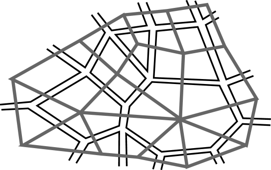
Figure 1: Part of a typical large Feynman diagram in an ${\rm SU}(N)$ gauge theory. A dual representation (gray lines) is obtained by associating a $p$-gon to each vertex of order $p$. The $p$-gons generate a discretized Riemann surface. The double scaling limits correspond to a continuum limit where the number of $p$-gons becomes infinite and thus the discretized Riemann surfaces become genuine smooth world sheets. The power of $\kappa^{2}\propto 1/N^{2}$ counts the genus of these world sheets.

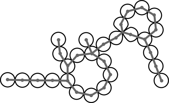
Figure 2: Part of a typical large Feynman diagram in the ${\mathbb{C}}P^{N}$ non-linear $\sigma$ model. A dual representation (gray lines) is obtained by associating a bound linking $p$ “molecules” (small gray disks) to each vertex of order $2p$. The bounds generate a discretized “polymer” with both forced (for bounds with $p\geq 3$) and dynamical branching. The double scaling limits correspond to a continuum limit where the number of bounds become infinite and thus the discretized polymers become genuine smooth world lines. The power of $\kappa\propto 1/N$ counts the number of loops (two in our example) of these world lines.

What do those diagrams look like? In the case of gauge theories (Figure 1), the answer [3] is that the diagrams contributing to a given order in $1/N^{2}$ can be mapped to discretized Riemann surfaces of a given genus. Large diagrams have a very large number of polygons, and thus the double scaling limit is a continuum limit for the discretized surfaces. We conclude that the resulting theory must be a string theory. For non-linear $\sigma$ models the analogous statements are easy to derive. In the case of linear $\sigma$ models [21], the typical large $N$ graphs are “bubble” diagrams, the order in $1/N$ being related to the number of loops of bubbles. In a dual representation (Figure 2), we obtain a discretized world line (or “polymer”) with a given number of loops. The double scaling limit is then a continuum limit for these discretized loop diagrams, and as a result we should obtain a standard field theory. The case of non-linear $\sigma$ models is similar, with the additional subtlety that we have interaction vertices of any order $p\geq 2$, but we still expect the resulting theory to be a field theory.

For the purposes of the calculations that follow, it is convenient to go to the euclidean for which $x^{2}=ix^{0}$ and $\partial\hbox to0.0pt{\hss/\hskip 0.2pt}_{\rm Eucl.}=-i\partial\hbox to0.0pt{\hss/\hskip 0.2pt}_{\rm Mink.}$. The euclidean lagrangian deduced from (2.1.2) is

$$\hskip-51.21504ptL_{\rm E}=-L=\sum_{i=1}^{N+1}\Bigl{(}\nabla_{\alpha}\phi_{i}^{\dagger}\,\nabla_{\alpha}\phi_{i}+|\sigma+m_{i}|^{2}\,|\phi_{i}|^{2}+\bar{\psi}_{i}\left(\nabla\hbox to0.0pt{\hss/\hskip 2.4pt}-\check{\sigma}-\check{m}\right)\psi_{i}\Bigr{)}+{i\theta\over 2\pi}\,*v$$

$$\hskip 42.67912pt-D\,\Bigl{(}\sum_{i=1}^{N+1}|\phi_{i}|^{2}-{4\pi\over g^{2}}\Bigr{)}-i\sqrt{2}\,\bar{\mu}\sum_{i=1}^{N+1}\psi_{i}\phi_{i}^{\dagger}+i\sqrt{2}\sum_{i=1}^{N+1}\phi_{i}\bar{\psi}_{i}\,\mu\,,$$ (4.5)

where we have defined the covariant derivative $\nabla_{\alpha}=\partial_{\alpha}+iv_{\alpha}$, the field strenght $*v=\partial_{1}v_{2}-\partial_{2}v_{1}$, and $\check{\sigma}=\mathop{\rm Re}\nolimits\sigma-i\sigma^{3}\mathop{\rm Im}\nolimits\sigma$, $\check{m}_{i}=\mathop{\rm Re}\nolimits m_{i}-i\sigma^{3}\mathop{\rm Im}\nolimits m_{i}$.

4.2 First class singularities

We consider the distribution (3.7) again. It is convenient to make the substitution $\sigma\rightarrow\sigma-v/(N+1)$ and to define

$$m=-v=\Lambda r,$$ (4.6)

in line with the notations of Section 3. The large $N$ limit is studied by integrating the superfields $\Phi_{i}=(\phi_{i},\psi_{i})$ from (4.1). This can be done exactly, and yields a non-local effective action proportional to $N$. The $1/N$ expansion is then a perturbative expansion for this non-local effective action. For the particular distribution (3.7), the superfield $\Phi_{N+1}$ plays a special rôle. One must actually keep this superfield explicitly in order to get a well-defined saddle point at large $N$. We are then left with a path integral over the fields $\phi=\phi_{N+1}/\sqrt{N}$, $\psi=\psi_{N+1}/\sqrt{N}$ and $\Sigma=(\sigma,\mu,D,v)$ which reads

$$\hskip-28.45274pt\int\!{\cal D}(\phi,\psi,\sigma,\mu,D,v_{\alpha})\,\left[{\mathop{\rm det}\nolimits_{\rm r}(\nabla\hbox to0.0pt{\hss/\hskip 2.4pt}-\check{\sigma})\over\mathop{\rm det}\nolimits_{\rm r}(-\nabla^{2}+|\sigma|^{2}-D-2\,\bar{\mu}(\nabla\hbox to0.0pt{\hss/\hskip 2.4pt}-\check{\sigma})^{-1}\mu)}\right]^{N}$$

$$\exp\Biggl{[}-N\int\!d^{2}x\,\Bigl{(}\nabla_{\alpha}\phi^{\dagger}\,\nabla_{\alpha}\phi+(|\sigma+m|^{2}-D)\,|\phi|^{2}+\bar{\psi}\left(\nabla\hbox to0.0pt{\hss/\hskip 2.4pt}-\check{\sigma}-\check{m}\right)\psi$$

$$\hskip 105.2751pt+{i\theta\over 2\pi N}\,*v+{D\over 2\pi}\ln{\mu\over|\Lambda|}-i\sqrt{2}\,\bar{\mu}\psi\phi^{\dagger}+i\sqrt{2}\phi\bar{\psi}\,\mu\,\Bigr{)}\Biggr{]}.$$ (4.7)

The renormalized determinants are studied in Appendix A, where all the formulas that we will use in the following can be found. The scale $\mu$ appearing in $\ln(\mu/|\Lambda|)$, not to be confused with the spinor $\mu$, is a renormalization scale appearing in the definition of the determinants.

4.2.1 The BPS/anti-BPS bound state

Before taking the scaling limit (3.15) on the full path integral (4.2), it is instructive to study explicitly an observable that has a non-trivial perturbative expansion, to complement the discussion of Section 3. We will consider the mass of a BPS/anti-BPS bound state that turns out to become massless at the first class singularity.

The saddle point equations for (4.2) are deduced from the effective potential

$$V_{\rm eff}=(|\sigma+m|^{2}-D)\,|\phi|^{2}+{D\over 2\pi}\ln{\mu\over|\Lambda|}+{|\sigma|^{2}\over 4\pi}\ln{|\sigma|^{2}\over e\mu^{2}}-{|\sigma|^{2}-D\over 4\pi}\ln{|\sigma|^{2}-D\over e\mu^{2}}\,\cdotp$$ (4.8)

The saddle points $dV_{\rm eff}=0$ correspond to the possible $N=\infty$ limit of the vacuum expectation values of the fields, and are also given by the condition $V_{\rm eff}=0$ by supersymmetry. Two cases must be considered. When $|r|=|m/\Lambda|<1$, the only solution is

$$\langle\phi\rangle=\langle D\rangle=0\,,\quad|\langle\sigma\rangle|=|\Lambda|\,.$$ (4.9)

We thus get an enhançon, as discussed in Section 3.1 or in more details in [1], which is simply a circle in the $\sigma$ plane. When $|r|>1$, in addition to the enhançon (4.9), we get another solution,

$$\langle D\rangle=0\,,\quad|\langle\phi\rangle|^{2}={1\over 2\pi}\ln{|m|\over|\Lambda|}\,\raise 2.0pt\hbox{,}\quad\langle\sigma\rangle=-m\,.$$ (4.10)

This solution corresponds to the root $x_{2}$ in equation (3.9), while the root $x_{1}$ of equation (3.8) lies on the enhançon (4.9). The critical point occurs when the two roots coincide.

The vacuum (4.10) is weakly coupled when $|m|\gg|\Lambda|$. In this regime, the relevant fields are the coordinates $\phi_{1}/\phi_{N+1},\ldots,\phi_{N}/\phi_{N+1}$ on ${\mathbb{C}}P^{N}$. They create BPS states of mass $|m|$. The field $\phi=\phi_{N+1}/\sqrt{N}$ plays the rôle of a Higgs field breaking the ${\rm U}(1)$ gauge symmetry (2.13). Choosing the unitary gauge and using (4.10), we write

$$\phi=\left({1\over 2\pi}\ln{|m|\over|\Lambda|}\right)^{1/2}\!\!+\varphi={2\sqrt{\pi}\over g(|m|)}+\varphi\,\raise 2.0pt\hbox{,}$$ (4.11)

where $\varphi$ is a fluctuating real scalar field. The constraint (2.12), which is valid in the vacuum (4.10), shows that $\varphi$ is a composite operator creating a two-particle BPS/anti-BPS bound state of the elementary quanta. Though the attractive force between these quanta is of order $1/N$ at large $N$, the mixing between the $N$ flavors will stabilize the bound state significantly, and the binding energy should be of order $N^{0}$. The mass $m_{\rm b}$ of this bound state is a nice example of an observable which has a highly non-trivial perturbative expansion, as opposed to the cases studied in Section 3. We can straightforwardly calculate the leading large $N$ approximation for $m_{\rm b}$, by looking at the quadratic piece of the effective action deduced from (4.2), see Appendix A. There is a mixing between $\varphi$ and the gauge multiplet. By inverting the matrix-valued propagator, we find a pole at $p^{2}=-m_{\rm b}^{2}$ such that

$$\ln\left|{m\over\Lambda}\right|={1+\sqrt{1+u^{2}}\over u}\arctan{1\over u}={8\pi^{2}\over\lambda_{\mu}^{2}}-{8\pi^{2}\over\lambda_{\mu,\rm c}^{2}}\,\raise 2.0pt\hbox{,}$$ (4.12)

where

$$u=\sqrt{{4|m|^{2}\over m_{\rm b}^{2}}-1}\,\,,\quad{8\pi^{2}\over\lambda_{\mu}^{2}}=\ln{\mu\over|\Lambda|}\,\raise 2.0pt\hbox{,}\quad{8\pi^{2}\over\lambda_{\mu,\rm c}^{2}}=\ln{\mu\over|m|}\,\cdotp$$ (4.13)

If we define perturbation theory in terms of the ’t Hooft coupling constant $\lambda^{2}_{\mu}$ with renormalization scale $\mu\geq|\Lambda|$, (4.12) implies an expansion

$$u={\lambda_{\mu}^{2}\over 8\pi}+\sum_{k=2}^{\infty}u_{\mu,k}\lambda^{2k}_{\mu}$$ (4.14)

with some $\mu$-dependent coefficients $u_{k}$. Near the critical point $m\rightarrow|\Lambda|$ or $\lambda_{\mu,\rm c}\rightarrow\lambda_{\mu}$, (4.12) implies

$$u\sim{\lambda_{\mu,\rm c}^{2}/(8\pi^{2})\over 1-\lambda_{\mu}^{2}/\lambda_{\mu,\rm c}^{2}}\,\cdotp$$ (4.15)

For the general picture of Section 4.1 to apply, one would need to prove that the series (4.14) has a radius of convergence

$$R_{\mu}=\lambda_{\mu,\rm c}\,,$$ (4.16)

or equivalently that

$$u_{\mu,k}\mathop{\sim}\limits_{k\rightarrow\infty}={\lambda_{\mu,\rm c}^{2(1-k)}\over 8\pi^{2}}\,\raise 2.0pt\hbox{,}$$ (4.17)

at least for a particular choice of $\mu$. This would indeed imply that the perturbative series (4.14) is dominated by the terms with large $k$, or equivalently by the large Feynman graphs, near the singularity. Proving (4.16), however, turns out to be particularly tricky. One can show rigorously that $R_{\mu}>0$ for all $\mu$, and that if $R_{\mu}=\lambda_{\mu,\rm c}$ for some particular $\mu$, then it is true for all larger values of $\mu$ as well. One can also show, using Picard theorem, that for $\mu=|\Lambda|$, which means $\lambda_{\mu,\rm c}=\infty$, the radius is actually finite, contradicting (4.16). To really understand what was going on, we performed a numerical analysis. For large enough values of $\mu$, such that $\lambda^{2}_{\mu,\rm c}/(8\pi^{2})\lesssim 0.45$, (4.17) is found to be satisfied, with a rapid and smooth convergence. For $\lambda^{2}_{\mu,\rm c}/(8\pi^{2})\gtrsim 0.45$, however, the behaviour of the coefficients $u_{\mu,k}$ changes drastically and (4.17) is apparently violated.

The perturbative series for the mass of the bound state itself can be immediately deduced from (4.14) and (4.13), and it has the same properties. At small coupling, we have

$$m_{\rm b}\simeq 2|m|\Bigl{(}1-{\lambda_{\mu}^{2}\over 2^{7}\pi^{2}}+{\cal O}(\lambda_{\mu}^{4})\Bigr{)}\,,$$ (4.18)

but near the critical points the high orders in perturbation theory dominate and we find

$$m_{\rm b}\propto{1\over u}\rightarrow 0\,.$$ (4.19)

It is important to realize that the asymptotic behaviours (4.15) or (4.19) do not depend on $\mu$, an obvious consequence of the renormalization group equations. If we introduce $\delta=r-1\sim\ln(m/\Lambda)$ as in (3.15), the asymptotics read

$$u\sim 1/|\delta|\,,\quad m_{\rm b}\sim 2|\Lambda\delta|\,.$$ (4.20)

This equation has two important consequences. First it shows that the BPS/anti-BPS bound state becomes massless at the critical point in the leading large $N$ approximation. This is a nice result, because usually only BPS states can be proven to become massless at such singularities, by using exact BPS mass formulas as the one discussed in Section 2 or 3 (in our example the massless BPS states are the solitons interpolating between the two vacua that “collide” at the critical point). Second, after doing the rescaling (4.1) for $p=1$ (the correct value for a first class singularity), the mass $m_{\rm b}$ is multiplied by $N$ (in the same way as the central charge was mutiplied my $N$, see (3.16)), and thus has a finite non-trivial limit in the double scaling (3.15) at leading order,

$$(Nm_{\rm b})_{\rm scaled}=2|\Lambda|/\kappa+{\cal O}(\kappa^{0})\,.$$ (4.21)

What about the higher orders in $1/N$? Can we trust the results obtained in the leading $1/N$ approximation? As we will show shortly, qualitatively, the answer is yes: the BPS/anti-BPS bound state does become massless, and $Nm_{\rm b}$ does have a non-trivial finite limit in the scaling (3.15). However, quantitatively, there are some important subtleties. The fact that $(Nm_{\rm b})_{\rm scaled}$ is finite to all orders and has a non-trivial expansion in $\kappa$ (a result we will prove in the next subsection) implies that the $1/N$ corrections to $m_{\rm b}$ must diverge at fixed $N$ when $\delta\rightarrow 0$. The leading order equation (4.20) is thus not to be trusted. The correct asymptotics is actually

$$m_{\rm b}\propto|\Lambda\delta^{3/2}|\,.$$ (4.22)

One must not be confused and conclude that, in the exact theory, (4.21) is wrong. Equation (4.22) is valid when $\delta\rightarrow 0$ at fixed $N$, while in the double scaling limit (3.15) we take $N\rightarrow\infty$ and $\delta\rightarrow 0$ in a correlated way. The result (4.22) and the fact that $(Nm_{\rm b})_{\rm scaled}$ has a non-trivial expansion in $\kappa$, far from being contradictory, actually complement each other. The non-trivial exponent in (4.22) is a consequence of the fact that the CFT at the critical point is non-trivial. This non-triviality is the cause of the divergences in the $1/N$ expansion. $(Nm_{\rm b})_{\rm scaled}$ in turn picks up the most IR divergent terms in this expansion (see also [1] for further discussion).

4.2.2 The double scaling limit

Showing that the scaling (3.15) is fully consistent might look like a very difficult task, because it amounts to resumming the most divergent terms in the $1/N$ expansion to all orders and beyond. What makes it possible, and even easy, is the IR nature of the divergences. Not surprisingly, and as equation (4.1) shows, this implies that the double scaling limit is also a low energy limit, and the path integral (4.2) simplifies considerably in such a limit. The same property makes tractable the case of linear $\sigma$ models [23], and was first used in the context of non-linear $\sigma$ models in [10].

The starting point of the proof is the non-local effective action defining the path integral (4.2). By rescaling $\phi\rightarrow\phi/\sqrt{N}$ and introducing the field $s=\sigma+m$ and the functionals $\xi$ and $\zeta$ discussed in Appendix A, it reads

$$\hskip-28.45274ptS_{\rm eff}=\int\!d^{2}x\,\Bigl{(}\nabla_{\alpha}\phi^{\dagger}\,\nabla_{\alpha}\phi+(|s|^{2}-D)\,|\phi|^{2}+{i\theta\over 2\pi}\,*v+{ND\over 2\pi}\ln{\mu\over|\Lambda|}\Bigr{)}$$

$$\hskip 42.67912pt+2N\,\xi\left[|s-m|^{2}-D,v_{\alpha}\right]-2N\,\zeta\left[-m+s,v_{\alpha}\right]+{\rm fermions}\,.$$ (4.23)

We will work thereafter with the bosonic fields only, the fermionic part of the action being unambiguously determined by supersymmetry. The rescaling of the space-time variables (4.1) $x^{\alpha}=N\sigma^{\alpha}$ implies that a quantity of dimension $D$ scale as $N^{-D}$. This means that the volume element $d^{2}x$ scales as $N^{2}$, the partial derivatives $\partial_{\alpha}$ and the fields $s$ and $v_{\alpha}$ scale as $1/N$, and the fields $D$ and $v_{\alpha\beta}$ scale as $1/N^{2}$. Moreover, (3.15) shows that $\delta$ scales like $1/N$. With those scalings, only a few terms in $S_{\rm eff}$ survive when $N\rightarrow\infty$. It is straightforward to check that those terms are at most linear in $D$ and $*v$, and at most cubic in $s$. Terms containing derivatives cannot survive, because Lorentz invariance implies that derivatives must come in pair, and the dominant term with derivatives, $\int(\partial s)^{2}$, goes like $N^{-1}$. These remarks imply that all the relevant terms in $S_{\rm eff}$ can be obtained from the potential (4.8) and from (A.9). Adding up all the contributions, and using $\arg m=\arg\Lambda+\mathop{\rm Im}\nolimits\delta$, we get

$$\hskip-42.67912ptS_{\rm eff}=\int_{|\Lambda|}\!d^{2}x\,\Bigl{(}\nabla_{\alpha}\phi^{\dagger}\,\nabla_{\alpha}\phi+(|s|^{2}-D)\,|\phi|^{2}+{ND\over 2\pi}\mathop{\rm Re}\nolimits(\delta-s/\Lambda)$$

$$\hskip 85.35826pt-{iN*v\over 2\pi}\mathop{\rm Im}\nolimits(\delta-s/\Lambda)+{\rm fermions}\Bigr{)}+{\cal O}(1/N).$$ (4.24)

This formula is strictly valid only with a cut-off $\sim N^{0}|\Lambda|$ that we have indicated on the integral sign, since we have been using a derivative expansion. The terms that potentially scale as $N^{2}$ or $N$ cancel, which is a necessary condition for the scaling (3.15) to be consistent. The terms cubic in $s$ also cancel, as a consequence of supersymmetry. Back to Minkowski space-time, and adding the fermions, (4.24) can be written as

$$S_{\rm eff}=\int_{|\Lambda|}\!d^{2}x\,\left[{1\over 4}\int\!d^{4}\theta\,\Phi^{\dagger}e^{2V}\Phi-{N\over 4\pi}\mathop{\rm Re}\nolimits\int\!d\theta_{-}d\bar{\theta}_{+}\Bigl{(}\delta\Sigma-{\Sigma^{2}\over 2\Lambda}\Bigr{)}\right]+{\cal O}(1/N).$$ (4.25)

It is useful at this point to introduce explicitly the scalings in $N$. This can be done in a manifestly supersymmetric way by defining

$$x^{\mu}=N\sigma^{\mu}\,,\quad\theta_{\pm}=\sqrt{N}\,\Theta_{\pm}\,,\quad\bar{\theta}_{\pm}=\sqrt{N}\,\bar{\Theta}_{\pm}\,,$$ (4.26)

which yield a new super field strenght

$$S=\bar{D}_{+,(\Theta,\sigma)}D_{-,(\Theta,\sigma)}V=N\bar{D}_{+,(\theta,x)}D_{-,(\theta,x)}V=N\Sigma\,$$ (4.27)

and an action

$$\hskip-4.26773ptS_{\rm eff}=\!\int_{N|\Lambda|}\!\!\!\!d^{2}\sigma\left[{1\over 4}\int\!d^{4}\Theta\,\Phi^{\dagger}e^{2V}\Phi-{1\over 4\pi}\mathop{\rm Re}\nolimits\int\!d\Theta_{-}d\bar{\Theta}_{+}\Bigl{(}N\delta\,S-{S^{2}\over 2\Lambda}\Bigr{)}\right]+{\cal O}(1/N).$$ (4.28)

The cut-off in the new space-time coordinates $\sigma$ is now of order $N$. Neglected terms, that all go to zero when $N\rightarrow\infty$, include for example the gauge and $s$ fields kinetic terms that may be deduced from (4.23),

$$-{N\over 32\pi|\Lambda|^{2}}\int\!d^{2}xd^{4}\theta\,\bar{\Sigma}\Sigma=-{1\over 32\pi|\Lambda|^{2}N}\int\!d^{2}\sigma d^{4}\Theta\,\bar{S}S\,.$$ (4.29)

Let us now actually take the limit $N\rightarrow\infty$ and $\delta\rightarrow 0$ in (4.28). Since the cut-off goes to infinity in this limit, one must renormalize the theory (4.28) in order to get a finite answer. This is the origin of the logarithmic correction to the naïve scaling in (3.15). Only a one-loop renormalization of the linear term in the twisted superpotential is needed, as can be checked by integrating out the superfield $\Phi$. One must add a counterterm $S(\ln(\Lambda_{0}/\mu))/(4\pi)$ to make the theory finite, where $\Lambda_{0}=N|\Lambda|$ is the cut-off for (4.28) and $\mu$ an arbitrary renormalization scale. This means that $N\delta$ is renormalized, with

$$N\delta=(N\delta)_{\rm r}+\ln{\Lambda_{0}\over\mu}=(N\delta)_{\rm r}+\ln{|\Lambda|\over\mu}+\ln N\,,$$ (4.30)

where $(N\delta)_{\rm r}=1/\kappa+\ln\kappa$ is the renormalized quantity to be held fixed when the cut-off is removed. We thus recover the scaling (3.15), and this completes the proof.

Several comments are here in order. First, it is important to understand the meaning of the “truncated” action (4.28), with respect to the full action (4.23). To do the ordinary $1/N$ expansion, one starts from (4.23) and expands around a saddle point, for example (4.9). An infinite number of vertices is then generated from (4.23), a vertex of order $p$ contributing with a power of $N^{1-p/2}$ by the standard large $N$ counting. The few terms that we have kept in (4.28) or (4.24), like the terms $|s|^{2}|\phi|^{2}$ or $-D|\phi|^{2}$, correspond to the vertices producing the most IR divergent contributions near the critical points, which are the only one that survive in the scaling (3.15). A second important comment is that the double scaled theory does not depend on a cut-off. It is a field theory consistent on all scales, defined by the action

$$S_{\rm scaled}=\!\int\!d^{2}\sigma\left[{1\over 4}\int\!d^{4}\Theta\,\Phi^{\dagger}e^{2V}\Phi-{1\over 4\pi}\mathop{\rm Re}\nolimits\int\!d\Theta_{-}d\bar{\Theta}_{+}\biggl{(}\Bigl{(}{1\over\kappa}+\ln\kappa+\ln{\Lambda_{0}\over\mu}\Bigr{)}S-{S^{2}\over 2\Lambda}\biggr{)}\right],$$ (4.31)

with the UV cut-off $\Lambda_{0}$ taken to infinity and renormalized coupling constant $\kappa$. Interestingly, the phenomenon of dimensional transmutation takes place, and the coupling $\kappa$ is actually replaced by a scale $M$ is the quantum theory,

$${1\over\kappa}+\ln\kappa=\ln{\mu\over M}\,\cdotp$$ (4.32)

The physics described by the action (4.31) depends on the dimensionless ratio

$$R=M/\Lambda\,.$$ (4.33)

By integrating out the superfield $\Phi$, one can deduce the effective superpotential $w$ by using (2.37),

$$w(s)={1\over 4\pi}\Bigl{[}s\ln{s\over eM}-{s^{2}\over 2\Lambda}\Bigr{]}={\Lambda\over 4\pi}\Bigl{[}u\ln{u\over eR}-{u^{2}\over 2}\Bigr{]}\raise 2.0pt\hbox{,}$$ (4.34)

with $s=\Lambda u$. We recover, up to a global factor, the result obtained in Section 3, equation (3.21). The double scaled theory has two vacua, obtained by solving $dw/du=0$. When $R=1/e$, the two vacua collide at $u=1$, and we get a critical point, which is nothing but the original critical point used to define the double scaling limit. By expanding around $u=1$, $S=\Lambda+T$, and by using the formulas of the Appendix, one can deduce the low energy effective action describing (4.31) near the critical point,

$$S_{\rm scaled,eff}=-\int_{|\Lambda|}\!d^{2}\sigma\left[{1\over 32\pi|\Lambda|^{2}}\int\!d^{4}\Theta\,T^{\dagger}T-{1\over 4\pi}\mathop{\rm Re}\nolimits\int\!d\Theta_{-}d\bar{\Theta}_{+}\Bigl{(}T\ln(eR)+{T^{3}\over 6\Lambda^{2}}\Bigr{)}\right].$$ (4.35)

Not surprisingly, we obtain a simple Landau-Ginzburg description of the $A_{1}$ minimal ${\cal N}=2$ CFT. Note that the double scaled theory (4.31), however, differ from this simple Landau-Ginzburg description at high energies.

Let us emphasize that the same qualitative phenomena are likely to occur in the gauge/string theory case at a first class singularity [2]. In particular, the string coupling should dissappear and be replaced by a mass scale.

4.3 Second class singularities

For the sake of simplicity and conciseness, we will study the case of the simplest critical point only, corresponding to $m=2$ in the notations of Section 3.3.2. Unlike the case of the first class singularity, we can integrate over all of the $N+1$ superfields $\Phi_{i}$ in (4.1), and we are left with the following path integral over $\Sigma$,

$$\hskip-17.07182pt\int\!{\cal D}(\sigma,\mu,D,v_{\alpha})\exp\Biggl{[}-(N+1)\int\!d^{2}x\,\Bigl{(}{D\over 2\pi}\ln{\mu\over|\Lambda|}+{i\theta\over 2\pi(N+1)}\,*v\Bigr{)}\Biggr{]}\times$$ (4.36)

$$\hskip-36.98866pt\left[{\mathop{\rm det}\nolimits_{\rm r}(\nabla\hbox to0.0pt{\hss/\hskip 2.4pt}-\check{\sigma}-\check{m})\mathop{\rm det}\nolimits_{\rm r}(\nabla\hbox to0.0pt{\hss/\hskip 2.4pt}-\check{\sigma}+\check{m})\over\mathop{\rm det}\nolimits_{\rm r}(-\nabla^{2}+|\sigma+m|^{2}-D-2\,\bar{\mu}F_{+}^{-1}\mu)\mathop{\rm det}\nolimits_{\rm r}(-\nabla^{2}+|\sigma-m|^{2}-D-2\,\bar{\mu}F_{-}^{-1}\mu)}\right]^{{\scriptstyle N+1\over\scriptstyle 2}}\hskip-19.91684pt\raise 2.0pt\hbox{,}$$

where $F_{\pm}=\nabla\hbox to0.0pt{\hss/\hskip 2.4pt}-(\check{\sigma}\pm\check{m})$. The effective potential is

$$\hskip-42.67912ptV_{\rm eff}={D\over 2\pi}\ln{\mu\over|\Lambda|}+{|\sigma+m|^{2}\over 8\pi}\ln{|\sigma+m|^{2}\over e\mu^{2}}+{|\sigma-m|^{2}\over 8\pi}\ln{|\sigma-m|^{2}\over e\mu^{2}}$$

$$-{|\sigma+m|^{2}-D\over 8\pi}\ln{|\sigma+m|^{2}-D\over e\mu^{2}}-{|\sigma-m|^{2}-D\over 8\pi}\ln{|\sigma-m|^{2}-D\over e\mu^{2}}\,\raise 2.0pt\hbox{,}$$ (4.37)

and yields the $N\rightarrow\infty$ vacuum expectation values

$$\langle D\rangle=0\,,\quad|\langle\sigma\rangle^{2}-m^{2}|=|\Lambda|^{2}\,.$$ (4.38)

The solution for $\sigma$ gives the enhançon that was described in the Figure 4 of [1]. The critical point is obtained when the two disconnected components of the enhançon collide, at $|m|=|\Lambda|$ and $\langle\sigma\rangle=0$.

To study the double scaling limit, we use the same strategy as in Section 4.2.2. We focus on the bosonic part of the action. The rescaling of the space-time variables is $x^{\alpha}=\sqrt{N}\sigma^{\alpha}$ (4.1), showing that $d^{2}x$ scales as $N$, the partial derivative $\partial_{\alpha}$ and the fields $\sigma$ and $v_{\alpha}$ scale as $1/\sqrt{N}$, and the fields $D$ and $v_{\alpha\beta}$ scale as $1/N$. As for the deviation from the critical point,

$$\delta=\ln{m^{2}\over\Lambda^{2}}\,\raise 2.0pt\hbox{,}$$ (4.39)

equation (3.31) shows that it scales as $1/N$. Those scalings imply that the only terms that can survive are either the kinetic term for $\sigma$ or the gauge field, that can be derived from (A.20) and (A.21), potential terms at most quartic in $\sigma$ and quadratic in $D$, that can be derived from (4.37), and terms linear in $v_{\alpha\beta}$ and at most quadratic in $\sigma$ that can be derived from (A.9). Adding up all the contributions, we get the action

$$\hskip-42.67912ptS_{\rm eff}=(N+1)\int_{|\Lambda|}\!d^{2}x\,\left[{1\over 8\pi|m|^{2}}\Bigl{(}{1\over 2}v_{\alpha\beta}v_{\alpha\beta}+\partial_{\alpha}\sigma^{\dagger}\partial_{\alpha}\sigma-D^{2}\Bigr{)}\right.$$

$$\hskip-14.22636pt\left.+{D\over 4\pi}\mathop{\rm Re}\nolimits(\delta-\sigma^{2}/m^{2})-{i*v\over 4\pi}\mathop{\rm Im}\nolimits(\delta-\sigma^{2}/m^{2})+{\rm fermions}\right]+{\cal O}(1/\sqrt{N}).$$ (4.40)

Introducing the scalings explicitly,

$$x^{\mu}=\sqrt{N}\sigma^{\mu}\,,\quad\theta_{\pm}=N^{1/4}\,\Theta_{\pm}\,,\quad\bar{\theta}_{\pm}=N^{1/4}\,\bar{\Theta}_{\pm}\,,\quad S=\sqrt{N}\,\Sigma\,,\quad N\delta=t\,,$$ (4.41)

(4.40) reduces to,

$$S_{\rm scaled}=-{1\over 8\pi}\int_{\Lambda_{0}}\!d^{2}\sigma\left[{1\over 4|\Lambda|^{2}}\int\!d^{4}\Theta\,\bar{S}S+\mathop{\rm Re}\nolimits\int\!d\Theta_{-}d\bar{\Theta}_{+}\Bigl{(}tS-{S^{3}\over 3\Lambda^{2}}\Bigr{)}\right].$$ (4.42)

No remormalization is needed for the action (4.42), and thus the cut-off $\Lambda_{0}=\sqrt{N}|\Lambda|$ can be removed. The double scaled theory for a second class singularity is thus given by a simple Landau-Ginzburg action, as was suggested in Section 3.3.2. It coincides at low energy with the first class double scaled theory (4.35), but differs from it in the UV.

5 ${\cal N}=1$ supersymmetric models

The purpose of the following brief Section is to emphasize the fact that the results obtained so far do not depend on supersymmetry. We focused on a supersymmetric model because our main goal was to make a comparison with the four dimensional supersymmetric gauge theories studied in [1, 2]. In fact, we believe that constructions of non-supersymmetric four dimensional non-critical strings could be made by using non-supersymmetric gauge theories with Higgs fields and adjusting the parameters in the Higgs potential to approach a critical point.

The ${\cal N}=2$ supersymmetric model we have studied in details in this paper was based on the classical potential (2.21) with the constraints (2.12, 2.13) on the complex fields $\phi_{i}$. It is natural to suspect that a very similar, but only ${\cal N}=1$ supersymmetric, model could be constructed for which the classical potential is

$$V_{\rm cl}={1\over 2}\sum_{i=1}^{N+1}(\sigma+m_{i})^{2}\,\phi_{i}^{2}\,,$$ (5.1)

with real fields $\phi_{i}$, $\sigma$ and mass parameters $m_{i}$, and constraint

$$\sum_{i=1}^{N+1}\phi_{i}^{2}={4\pi\over g^{2}}\,\cdotp$$ (5.2)

Such a model indeed exists. By introducing Majorana spinors $\psi_{i}$ which are in the same supermultiplet as the $\phi_{i}$s and a supermultiplet $(\mu,D)$ of Lagrange multipliers, its lagrangian reads

$$\hskip-42.67912ptL=\sum_{i=1}^{N+1}\Bigl{(}{1\over 2}\,\phi_{i}\left(\partial^{2}-(\sigma+m_{i})^{2}\right)\phi_{i}^{2}+\bar{\psi}_{i}\left(i\partial\hbox to0.0pt{\hss/\hskip 0.2pt}+\sigma+m_{i}\right)\psi_{i}\Bigr{)}$$

$$\hskip 142.26378pt+{D\over 2}\,\Bigl{(}\sum_{i=1}^{N+1}\phi_{i}^{2}-{4\pi\over g^{2}}\Bigr{)}-\bar{\mu}\sum_{i=1}^{N+1}\psi_{i}\phi_{i}\,.$$ (5.3)

This is a $S^{N}$ non-linear $\sigma$ model with ${\cal N}=1$ supersymmetry. The mass terms come from a superpotential

$$W(\Phi_{i})={1\over 2}\sum_{i=1}^{N+1}m_{i}\Phi_{i}^{2}\,.$$ (5.4)

The lagrangian (5.3) is very similar to (2.1.2), and the large $N$ limit can be studied with the same methods [24]. A particularly interesting aspect of the model (5.3) is that the number of vacua changes when the mass parameters are varied, while the Witten index $\mathop{\rm tr}\nolimits(-1)^{F}=1+(-1)^{N}$ is, of course, constant. In the ${\mathbb{C}}P^{N}$ model, holomorphicity was preventing such drastic changes in the space of vacua. At large $N$, one can show that (2.35) is replaced by

$$\prod_{i=1}^{N+1}(\sigma+m_{i})^{2}=\Lambda^{2(N+1)}\,,$$ (5.5)

where all the parameters are now real. In the $\Lambda\rightarrow 0$ weak coupling limit, we have $2(N+1)$ vacua coming in $N+1$ inequivalent pairs,

$$\langle\sigma\rangle_{\rm w.c.}\simeq-m_{i}\,,\quad\langle\phi_{j}\rangle_{\rm w.c.}\simeq\pm{2\sqrt{\pi}\delta_{ij}\over g}\,\raise 2.0pt\hbox{,}$$ (5.6)

while at strong coupling we are left with only two vacua

$$\langle\sigma\rangle_{\rm s.c.}\simeq\pm\Lambda\,.$$ (5.7)

The particular values of the mass parameters for which the number of vacua changes correspond to critical points where the large $N$ expansion breaks down, and where double scaling limits can be defined. The double scaled theories are typically simple Landau-Ginzburg theories [24]. The scalings always look like (3.15), with logarithmic correction, because ${\cal N}=1$ Landau-Ginzburg models need to be renormalized by normal ordering the superpotential.

Instead of considering superpotential-induced mass terms, one can also use the isometries of the target space, as was done for the ${\mathbb{C}}P^{N}$ model. In that case, the ${\cal N}=1$ supersymmetric lagrangian takes the form

$$\hskip-42.67912ptL=\sum_{k,l=1}^{N+1}\Bigl{(}{1\over 2}\,\phi_{k}\left((\partial^{2}-\sigma^{2})\delta_{kl}-\smash{\sum_{i=1}^{N+1}}m_{ik}m_{il}\right)\phi_{l}^{2}+\bar{\psi}_{k}\left((i\partial\hbox to0.0pt{\hss/\hskip 0.2pt}+\sigma)\delta_{kl}+m_{kl}\sigma^{3}\right)\psi_{l}\Bigr{)}$$

$$\hskip 170.71652pt+{D\over 2}\,\Bigl{(}\sum_{i=1}^{N+1}\phi_{i}^{2}-{4\pi\over g^{2}}\Bigr{)}-\bar{\mu}\sum_{i=1}^{N+1}\psi_{i}\phi_{i}\,,$$ (5.8)

where $m_{ij}$ is an antisymmetric mass matrix. Again, critical points can be found, and double scaling limits defined [24]. An interesting aspect of the model (5.8) is that supersymmetry can be spontaneously broken when $N$ is odd.

In both models (5.3) and (5.8), the masses induce a quadradic term $h_{ij}\phi_{i}\phi_{j}/2$, where the tensor “magnetic field” ${\mathbf{h}}=\mathbf{m}\mathbf{m}^{T}$ is expressed in term of a symmetric or antisymmetric mass matrix respectively. One cannot find a supersymmetric theory with arbitrary $\mathbf{h}$, but the corresponding non-supersymmetric model can also be studied, and again critical points are found and double scaling limits can be defined [10].

6 Prospects

The main goal of the present paper was to improve one’s understanding of the results obtained in [1, 2]. We hope that our analysis has convinced the reader that the gauge theories double scaling limits are likely to yield well-defined four dimensional non-critical string theories, as conjectured in [2]. A natural avenue for future work is to try to generalize the cases studied in [2]. There is a variety of critical points appearing on the moduli space of supersymmetric gauge theories, and a large class of string theories can certainly be generated. Remarkably, for all those theories, the dimensions of the world sheet couplings as well as the space-time central charge as a function of these couplings can be calculated exactly. It would be interesting to study in details the structure of the formulas so obtained. One may hope, from experience with the $c<1$ matrix models where the KdV hierarchy plays a prominent rôle [22], that a general mathematical structure could emerge. Unravelling this structure might eventually help in understanding our string theories from a more conventional, ‘continuous’ point of view.

Another fascinating possible direction of research is based on the fact, explained in the Introduction, that our two dimensional models admit brane constructions. A crucial feature is that the large $N$ limit of the $\sigma$ models correspond to a large number of branes, as in the case of gauge theories [25]. One might then expect to be able to find a description involving quantum gravity. The startling point is that, in sharp contrast with the gauge theory case, the large $N$ limits of our models are exactly solvable.

Appendix A Formulas for determinants

We consider the renormalized euclidean determinants

$$\mathop{\rm det}\nolimits_{\rm r}(-\nabla^{2}+h)=\exp(2\,\xi[h,v_{\alpha}])\,,\quad\mathop{\rm det}\nolimits_{\rm r}(\nabla\hbox to0.0pt{\hss/\hskip 2.4pt}-\check{f})=\exp(2\,\zeta[f,v_{\alpha}])\,,$$ (A.1)

where the functionals $\xi$ and $\zeta$ are defined by the equations

$$\xi[h,v_{\alpha}]={1\over 2}\mathop{\rm tr}\nolimits\ln(-\nabla^{2}+h)-\xi_{0}[h,v_{\alpha}]\,,$$ (A.2)

$$\zeta[f,v_{\alpha}]={1\over 2}\mathop{\rm tr}\nolimits\ln(\nabla\hbox to0.0pt{\hss/\hskip 2.4pt}-\check{f})-\zeta_{0}[f,v_{\alpha}]\,,$$ (A.3)

with local counterterms $\xi_{0}$ and $\zeta_{0}$. The covariant derivative is $\nabla_{\alpha}=\partial_{\alpha}+iv_{\alpha}$, $h$ is a real and positive field, and $f$ is a complex field with associated matrix $\check{f}=\mathop{\rm Re}\nolimits f-i\sigma^{3}\mathop{\rm Im}\nolimits f$. The local counterterms depend on the regularization and renormalization schemes. Gauge invariant and supersymmetric results can be obtained by using a Pauli-Villars regularization with cut-off $\Lambda_{0}$, renormalization scale $\mu$ and counterterms

$$\xi_{0}={1\over 4\pi}\ln{\Lambda_{0}\over\mu}\,\int\!d^{2}x\,h\,,\quad\zeta_{0}={1\over 4\pi}\ln{\Lambda_{0}\over\mu}\,\int\!d^{2}x\,|f|^{2}\,.$$ (A.4)

Dimensional regularization $D=2-\epsilon$ can also be used, with the definition

$${1\over 2\pi}\ln{\Lambda_{0}\over\mu}=\int\!{d^{D}p\over(2\pi)^{D}}\,{1\over p^{2}+\mu^{2}}={1\over 2\pi\epsilon}-{1\over 4\pi}\ln{\mu^{2}\over 4\pi}-{\gamma\over 4\pi}\,\raise 2.0pt\hbox{,}$$ (A.5)

but one must add a finite local counterterm $-\int d^{2}x(\mathop{\rm Im}\nolimits f)^{2}/(4\pi)$ to the fermionic functional for supersymmetry to be preserved (such a term is generated due to the unusual properties of the $\bar{\psi}\sigma^{3}\psi\mathop{\rm Im}\nolimits f$ vertex in dimensional regularization).

A.1 Special cases

For $v_{\alpha}$ pure gauge, $h$ constant and positive, and $f$ constant, we have

$$\hskip-5.69046pt\xi[h={\rm cst}>0,v_{\alpha}=\partial_{\alpha}\chi]=\int\!d^{2}x\,V_{\rm b}(h)\,,\quad\zeta[f={\rm cst},v_{\alpha}=\partial_{\alpha}\chi]=\int\!d^{2}x\,V_{\rm f}(f)\,,$$ (A.6)

with the potentials

$$V_{\rm b}(h)=-{h\over 8\pi}\ln{h\over e\mu^{2}}\,\raise 2.0pt\hbox{,}\quad V_{\rm f}(f)=V_{\rm b}(|f|^{2})\,.$$ (A.7)

If $f=0$, we have, for any $v_{\alpha\beta}$ going to zero fast enough at infinity ,

$$\zeta[f=0,v_{\alpha}]={1\over 8\pi}\int\!d^{2}x\,v_{\alpha\beta}\,{1\over\partial^{2}}\,v_{\alpha\beta}\,.$$ (A.8)

If $\mathop{\rm Im}\nolimits f/\mathop{\rm Re}\nolimits f$ is constant, the term linear in $v_{\alpha\beta}$ in $\zeta$ can also be exactly calculated,

$$\zeta[f,v_{\alpha}]_{{\rm linear\ in\ }\tilde{v}}={i\over 8\pi}\int\!d^{2}x\,\epsilon_{\alpha\beta}v_{\alpha\beta}\,\mathop{\rm Im}\nolimits\ln f\,\cdotp$$ (A.9)

A.2 General case

In general, one writes

$$h=m^{2}+\varphi\,,\quad f=M+\phi\,,$$ (A.10)

with $m$ real and $M$ complex, and one expands the functionals in powers of the fields $\varphi$, $\phi$ and $v_{\alpha}$,

$$\xi[h,v_{\alpha}]=\sum_{n=0}^{\infty}\xi_{n}[\varphi,v_{\alpha};m^{2}]\,,\quad\zeta[f,v_{\alpha}]=\sum_{n=0}^{\infty}\zeta_{n}[\phi,v_{\alpha};M]\,.$$ (A.11)

The functionals

$$\xi_{1}={1\over 8\pi}\ln{\mu^{2}\over m^{2}}\int\!d^{2}x\,\varphi\,,$$ (A.12)

$$\zeta_{1}={i\over 8\pi}\int\!d^{2}x\,\epsilon_{\alpha\beta}v_{\alpha\beta}\mathop{\rm Im}\nolimits\ln M+{1\over 2\pi}\ln{\mu\over|M|}\int\!d^{2}x\,\mathop{\rm Re}\nolimits(M^{*}\phi)\,,$$ (A.13)

are linear in the fields, $s_{2}$ and $\zeta_{2}$ are quadratic, etc…The quadradic pieces are most easily expressed by introducing the Fourier transforms of the fields,

$$\hat{v}_{\alpha}(k)=\int\!d^{2}x\,e^{-ikx}v_{\alpha}(x)\,,\quad{\rm etc,}$$ (A.14)

and the one-loop integral

$$S(k;m^{2})=-{1\over 8\pi^{2}}\int{d^{2}p\over(p^{2}+m^{2})((p+k)^{2}+m^{2})}\,\cdotp$$ (A.15)

This integral can be evaluated in different regimes (euclidean, and below or above the pair production threshold), by using Feynman’s $i\epsilon$ prescription when necessary,

$$S(k;m^{2})=\left\{\matrix{-{\displaystyle 1\over\displaystyle 4\pi}\,{\displaystyle 1\over\displaystyle p^{2}\sqrt{1+4m^{2}/p^{2}}}\,\ln{\displaystyle\sqrt{1+4m^{2}/p^{2}}+1\over\displaystyle\sqrt{1+4m^{2}/p^{2}}-1}\,\raise 2.0pt\hbox{,}\ {\rm for\ }p^{2}>0\,,\hfill\cr\vskip 3.0pt plus 1.0pt minus 1.0pt\cr{\displaystyle 1\over\displaystyle 2\pi}\,{\displaystyle 1\over\displaystyle p^{2}\sqrt{-1-4m^{2}/p^{2}}}\,\arctan{\displaystyle 1\over\displaystyle\sqrt{-1-4m^{2}/p^{2}}}\,\raise 2.0pt\hbox{,}\ {\rm for\ }0<-p^{2}<4m^{2}\,,\hfill\cr\vskip 3.0pt plus 1.0pt minus 1.0pt\cr-{\displaystyle 1\over\displaystyle 4\pi}\,{\displaystyle 1\over\displaystyle p^{2}\sqrt{1+4m^{2}/p^{2}}}\,\left(\ln{\displaystyle 1+\sqrt{1+4m^{2}/p^{2}}\over\displaystyle 1-\sqrt{1+4m^{2}/p^{2}}}-i\pi\right)\!,\ {\rm for\ }-p^{2}>4m^{2}.\hfill\cr}\right.$$ (A.16)

Introducing $\phi_{1}(x)=\mathop{\rm Re}\nolimits\phi(x)$, $\phi_{2}(x)=\mathop{\rm Im}\nolimits\phi(x)$, $M_{1}=\mathop{\rm Re}\nolimits M$ and $M_{2}=\mathop{\rm Im}\nolimits M$, we have

$$\hskip-34.14322pt\xi_{2}={1\over 2}\int\!{d^{2}k\over(2\pi)^{2}}\Biggl{[}\Bigl{(}(k^{2}+4m^{2})S(k;m^{2})+{1\over 2\pi}\Bigr{)}\Bigl{(}{k_{\alpha}k_{\beta}\over k^{2}}-\delta_{\alpha\beta}\Bigr{)}\hat{v}_{\alpha}(-k)\hat{v}_{\beta}(k)$$

$$\hskip 220.50885pt+S(k;m^{2})\hat{\varphi}(-k)\hat{\varphi}(k)\Biggr{]}\,,$$ (A.17)

$$\hskip-34.14322pt\zeta_{2}={1\over 2}\int\!{d^{2}k\over(2\pi)^{2}}\Biggl{[}\Bigl{(}4|M|^{2}S(k;|M|^{2})+{1\over 2\pi}\Bigr{)}\Bigl{(}{k_{\alpha}k_{\beta}\over k^{2}}-\delta_{\alpha\beta}\Bigr{)}\hat{v}_{\alpha}(-k)\hat{v}_{\beta}(k)$$

$$\hskip 71.13188pt+\Bigl{(}(k^{2}+4M_{1}^{2})S(k;|M|^{2})+{1\over 2\pi}\ln{\mu\over|M|}\Bigr{)}\hat{\phi}_{1}(-k)\hat{\phi}_{1}(k)$$

$$\hskip 71.13188pt+\Bigl{(}(k^{2}+4M_{2}^{2})S(k;|M|^{2})+{1\over 2\pi}\ln{\mu\over|M|}\Bigr{)}\hat{\phi}_{2}(-k)\hat{\phi}_{2}(k)$$

$$\hskip 71.13188pt+4S(k;|M|^{2})\epsilon_{\alpha\beta}k_{\beta}\,\hat{v}_{\alpha}(-k)(M_{1}\hat{\phi}_{2}(k)-M_{2}\hat{\phi}_{1}(k))$$

$$\hskip 71.13188pt+8M_{1}M_{2}S(k;|M|^{2})\,\hat{\phi}_{1}(-k)\hat{\phi}_{2}(k)\Biggr{]}.$$ (A.18)

The low energy expansion up to two derivative terms is obtained by using

$$S(k;m^{2})=-{1\over 8\pi m^{2}}\,\Bigl{(}1-{k^{2}\over 6m^{2}}+{\cal O}(k^{4})\Bigr{)}$$ (A.19)

and it reads

$$\hskip-42.67912pt\xi_{2}^{\rm l.e.}={1\over 48\pi m^{2}}\int\!d^{2}x\,\Biggl{[}{1\over 2}v_{\alpha\beta}v_{\alpha\beta}+{1\over 2m^{2}}\partial_{\alpha}\varphi\partial_{\alpha}\varphi-3\varphi^{2}\Biggr{]},$$ (A.20)

$$\hskip-42.67912pt\zeta_{2}^{\rm l.e.}={1\over 48\pi|M|^{2}}\int\!d^{2}x\,\Biggl{[}-v_{\alpha\beta}v_{\alpha\beta}+6i\mathop{\rm Im}\nolimits(M^{*}\phi)\epsilon_{\alpha\beta}v_{\alpha\beta}-3\,\partial_{\alpha}\phi^{\dagger}\partial_{\alpha}\phi$$

$$\hskip-14.22636pt+{2\over|M|^{2}}\mathop{\rm Re}\nolimits(M\partial_{\alpha}\phi)\mathop{\rm Re}\nolimits(M\partial_{\alpha}\phi)+12|M\phi|^{2}\ln{\mu\over|M|}-12\left(\mathop{\rm Re}\nolimits(M^{*}\phi)\right)^{2}\Biggr{]}.$$ (A.21)

References

- [1] F. Ferrari, Nucl. Phys. B 612 (2001) 151.
- [2] F. Ferrari, Nucl. Phys. B 617 (2001) 348.
- [3] G. ’t Hooft, Nucl. Phys. B 72 (1974) 461.
- [4] É. Brézin, C. Itzykson, G. Parisi and J.B. Zuber, Comm. Math. Phys. 59 (1978) 35.
-
[5]
F. David, Nucl. Phys. B 257 (1985) 45,
V.A. Kazakov, Phys. Lett. B 150 (1985) 282,
J. Ambjörn, B. Durhuus and J. Fröhlich, Nucl. Phys. B 257 (1985) 433. -
[6]
É. Brézin and V.A. Kazakov, Phys. Lett. B 236 (1990) 144,
M.R. Douglas and S. Shenker, Nucl. Phys. B 355 (1990) 635,
D.J. Gross and A.A. Migdal, Phys. Rev. Lett. 64 (1990) 127. -
[7]
N. Seiberg and E. Witten, Nucl. Phys. B 426 (1994) 19, erratum
B 430 (1994) 485,
N. Seiberg and E. Witten, Nucl. Phys. B 431 (1994) 484. -
[8]
P. C. Argyres and A. E. Faraggi,
Phys. Rev. Lett. 74 (1995) 3931,
A. Klemm, W. Lerche, S. Yankielowicz and S. Theisen, Phys. Lett. B 344 (1995) 169. - [9] N. Dorey, J. High Energy Phys. 11 (1998) 005.
-
[10]
F. Ferrari, Phys. Lett. B 496 (2000) 212,
F. Ferrari, J. High Energy Phys. 6 (2001) 57. - [11] E. Witten, Nucl. Phys. B 500 (1997) 3.
- [12] A. Hanany and K. Hori, Nucl. Phys. B 513 (1998) 119.
- [13] N. Dorey, T.J. Hollowood and D. Tong, J. High Energy Phys. 5 (1999) 6.
-
[14]
F. Ferrari and A. Bilal, Nucl. Phys. B 469 (1996) 387,
A. Bilal and F. Ferrari, Nucl. Phys. B 480 (1996) 589,
F. Ferrari, Nucl. Phys. B 501 (1997) 53,
A. Bilal and F. Ferrari, Nucl. Phys. B 516 (1998) 175. -
[15]
L. Álvarez-Gaumé and D.Z. Freedman,
Comm. Math. Phys. 80 (1981) 443,
L. Álvarez-Gaumé and D.Z. Freedman, Comm. Math. Phys. 91 (1983) 87. - [16] S. Cecotti, P. Fendley, K. Intriligator and C. Vafa, Nucl. Phys. B 386 (1992) 405.
- [17] F. Ferrari, A note on theta dependence, NEIP-01-010, PUPT-2007, LPTENS-01/36, hep-th/0111117, to appear in Phys. Lett. B.
- [18] C.V. Johnson, A.W. Peet and J. Polchinski, Phys. Rev. D 61 (2000) 86001.
- [19] P.C. Argyres and M.R. Douglas, Nucl. Phys. B 448 (1995) 93.
-
[20]
F. David, Nucl. Phys. B 257 (1985) 45,
V.A. Kazakov, Phys. Lett. B 150 (1985) 282,
J. Ambjørn, B. Durhuus and J. Fröhlich, Nucl. Phys. B 257 (1985) 433. -
[21]
J. Ambjørn, B. Durhuus, and T. Jónsson,
Phys. Lett. B 244 (1990) 403,
S. Nishigaki and T. Yoneya, Nucl. Phys. B 348 (1991) 787,
P. Di Vecchia, M. Kato, and N. Ohta, Nucl. Phys. B 357 (1991) 495. - [22] P. Di Francesco, P. Ginsparg and J. Zinn-Justin, Phys. Rep. 254 (1995) 1.
-
[23]
G. Eyal, M. Moshe, S. Nishigaki and J. Zinn-Justin,
Nucl. Phys. B 470 (1996) 369,
M. Moshe, Quantum field theory in singular limits, Les Houches lecture 1997, hep-th/9812029,
J. Zinn-Justin, Vector models in the large limit: a few applications, lectures at the 11th Taiwan Spring School on Particles and Fields 1997, hep-th/9810198. - [24] F. Ferrari, unpublished.
-
[25]
J. Maldacena, Adv. Theor. Math. Phys. 2 (1998) 231,
S. Gubser, I.R. Klebanov and A.M. Polyakov, Phys. Lett. B 428 (1998) 105,
E. Witten, Adv. Theor. Math. Phys. 2 (1998) 253.