Strong Brane Gravity and the Radion at Low Energies

Abstract

For the 2-brane Randall-Sundrum model, we calculate the bulk geometry for strong gravity, in the low matter density regime, for slowly varying matter sources. This is relevant for astrophysical or cosmological applications. The warped compactification means the radion can not be written as a homogeneous mode in the orbifold coordinate, and we introduce it by extending the coordinate patch approach of the linear theory to the non-linear case. The negative tension brane is taken to be in vacuum. For conformally invariant matter on the positive tension brane, we solve the bulk geometry as a derivative expansion, formally summing the ‘Kaluza-Klein’ contributions to all orders. For general matter we compute the Einstein equations to leading order, finding a scalar-tensor theory with $\omega(\Psi)\propto\Psi/(1-\Psi)$, and geometrically interpret the radion. We comment that this radion scalar may become large in the context of strong gravity with low density matter. Equations of state allowing $(\rho-3P)$ to be negative, can exhibit behavior where the matter decreases the distance between the 2 branes, which we illustrate numerically for static star solutions using an incompressible fluid. For increasing stellar density, the branes become close before the upper mass limit, but after violation of the dominant energy condition. This raises the interesting question of whether astrophysically reasonable matter, and initial data, could cause branes to collide at low energy, such as in dynamical collapse.

1 Introduction

Much progress has been made in understanding the long range gravitational response of branes at orbifold fixed planes, to localized matter. The Randall-Sundrum models, with one or two branes [1, 2, 3] simply have gravity and a cosmological constant in the bulk, making the linear problem very tractable. Linear calculations [4, 5, 6, 7] show that in the one brane case, long range $4$-dimensional gravity is recovered on the brane. Little is known of the general non-linear behavior [8, 9]. There is no mass gap, and thus the non-linear problem is essentially a 5-dimensional one, even for long wavelength sources. Second order perturbation theory [10, 11], and fully non-linear studies [12, 13] are again consistent with recovering usual 4-dimensional strong gravity. In particular [12] shows that non-perturbative phenomena, such as the upper mass limit for static stars, extend smoothly from large to small objects, whose characteristic sizes are taken relative to the AdS length.

For the two brane case, linear theory [4] found that the effective gravity is Brans-Dicke, for an observer on the positive tension brane, and a vacuum negative tension brane. For reasonable brane separations phenomenologically acceptable gravity is recovered. For observers on the negative tension brane it was found the response was incompatible with observation for any brane separation, although stabilizing the distance between the branes does allow one to recover standard 4-dimensional gravity [14, 15, 16, 17, 18, 19, 20]. In this paper we consider an observer on the positive tension brane, the negative tension brane to be in vacuum, and the orbifold radius to be unstabilized. This allows us to study the dynamics of the radion in strong gravity. Of course, our methods may be extended to include the stabilized case too. Although moduli have previously been assumed to be fixed at late times, a crucial feature of the recent cyclic Ekpyrotic scenario [21, 22], is that the radius of the orbifold is not stabilized, the cyclic nature of this model being such that the separation always remains finite.

The two brane strong gravity case appears more tractable than for one brane, as the linear theory allows a Kaluza-Klein style reduction of the propagator [4]. In Kaluza-Klein compactifications, only the homogeneous zero modes are excited on long wavelengths, and the matter is thought to comprise fields over the whole internal space. However, for matter to be supported on the orbifold branes there must be modes excited which are not homogeneous in the extra dimension. Thus one cannot simply write down a non-linear ansatz for the metric, as is familiar from Kaluza-Klein compactifications.

In previous work on the Horava-Witten compactification [23], the low energy, long range effective theory was constructed using consistent orbifold reductions [24, 25, 26, 27, 28]. The methods developed treated the homogeneous component of the metric as a background, and inhomogeneous perturbations about it as the contribution of the massive ‘Kaluza-Klein’ modes. The metric was then solved to leading order in a derivative expansion. Strong gravity was not discussed in these works except when considering inflation [28]. In order to use these constructions, all the zero modes of the orbifold must be homogeneous. One important result of the warped compactification, is that whilst the graviton modes are homogeneous, the radion zero mode is not [29]. This appears to be a general feature of warped models [30, 31, 32], and one cannot directly use these Horava-Witten methods.

The aim of this paper is to apply the orbifold reduction to the warped Randall-Sundrum model, and then examine the non-linear behavior of the radion. We begin in section 2 by illustrating the reduction proposed in [24, 25, 26, 27, 28] with a field theory example and discuss its application to strong gravity. In order to apply the method we must find a way to include the inhomogeneous radion zero mode. Instead of explicitly using an ansatz including the radion, we include it by ‘deflecting’ the brane relative to a non-linear extension of the ‘Randall-Sundrum gauge’ [4, 5]. In sections 4 and 5 we solve the bulk metric for conformally invariant, low energy, long wavelength matter on the positive tension brane. For conformally invariant matter, this coordinate system is Gaussian normal to the brane. The bulk geometry is constructed using a derivative expansion, which is formally summed to all orders.

In section 6, we extend the linear analysis to the non-linear, for general low density, long wavelength matter, allowing the brane to become deflected relative to this coordinate system. This scalar deflection becomes the radion, and is treated non-linearly. This is crucial, as this field takes values roughly of order the Newtonian potential, for static systems. Therefore, the case of strong gravity is exactly where the radion must be treated non-linearly. We calculate a local action for the effective induced Einstein equations, to leading order in the derivative expansion. The resulting theory is a scalar-tensor model, which reduces to Brans-Dicke in the linear approximation. This is the first non-linear, covariant derivation of the effective action. Considering the zero modes [33] does not tell one the conformal metric that matter couples to. Whilst cosmological solutions such as [17, 15, 34, 35] may derive radion dynamics, this only applies for a homogeneous radion, and thus is not a covariant derivation. Indeed the examples [17, 15] illustrate this point well. The form of the metric chosen, whilst coincidentally reproducing the correct effective action [33], does not solve the correct linearized equations [29], and thus only applies to the case of cosmological symmetry.

We discuss in detail the validity of the approximation for considering low density, long wavelength strong brane gravity. Terms that are quadratic in the energy density are neglected in the orbifold reduction method, consistent with the low energy approximation. The characteristic length scale of the matter must be large compared to the compactification scale for the derivative expansion to be valid. For strong gravity, the approximation then holds provided the 4-dimensional induced brane curvature invariants are small, compared to the compactification scales. Thus this method will not allow a global solution to a black hole geometry, or any other spacetimes with curvature singularities. However, it will apply to all other cases of strong gravity, such as static relativistic stars, an example being neutron stars, or dynamical non-linear systems, such as binary neutron star systems, or collapse of matter up to the point where curvatures become singular.

Having pointed out that the radion may take large values for strong gravity configurations, we illustrate this using the example of relativistic stars. Previous work [36, 37] has considered stars on branes using the projection formalism of [38], allowing the quadratic stress tensor corrections to be calculated by making ansatzes on the bulk geometry. However, these corrections are assumed to be negligible in our low energy density assumption, and it is the bulk geometric corrections which are relevant, and cannot be calculated in the projection approach. In [12] the full bulk solutions were numerically constructed for the one brane Randall-Sundrum case. Using the methods here, we are able to analytically construct the geometry for large stars in the 2-brane case. In section 9, using the leading order action, we numerically consider the static relativistic star, for incompressible fluid matter. The linear theory shows that for perturbative stars with positive density the branes are deflected apart. However, it indicates that if $\rho-3P$ becomes negative the opposite could occur. Now understanding the radion and bulk geometry non-linearly, we consider this, finding that as non-linear effects become important the branes do indeed become closer. Furthermore, the branes appear to meet before the upper mass limit is reached. This will occur for any brane separation. However, for phenomenologically acceptable separations [4], we find it does not occur before the dominant energy condition is violated. Neutron stars are believed to have polytropic equations of state that do not support negative $\rho-3P$. It then remains a very interesting, and tractable $1+1$ problem to understand whether dynamical systems may cause branes to collide, for realistic matter and initial data. We then have the possibility that physical matter at low energies and curvatures, compared to compactification scales, might cause brane collisions requiring a Planck energy physics description.

2 Orbifold Reduction: A Field Theory Example

We illustrate the method of consistent orbifold reduction using a simple scalar field theory. The method was originally used in the context of Horava-Witten reductions [24, 25, 26, 27, 28]. We take the scalar equation,

$$\square_{d}\Psi+(\partial_{\mu}\Psi)^{2}+\partial_{y}^{2}\Psi+(\partial_{y}\Psi)^{2}=0$$ (1)

in a Minkowski $(d+1)$-dimensional bulk with signature $-,+,+,\ldots$ and coordinates $x^{\mu},y$, with $\mu=0,1,\ldots(d-1)$. We consider a finite range for $y$, choosing units such that $0\leq y\leq 1$. The operator $\square_{d}$ is the Laplacian on $d$-dimensional Minkowski space formed from $x^{\mu}$. The analogy of a Kaluza-Klein compactifications is to use periodic boundary conditions in $y$, identifying the field at $y=0$ and $y=1$. For orbifold brane compactifications the boundary conditions to consider are Neumann, with the field gradient $\partial_{y}\Psi=\rho(x)$ at $y=0$ and being zero gradient at $y=1$. This will later correspond to the case of matter on the positive tension brane, and a vacuum negative tension brane. The zero modes of the system, with $\rho(x)=0$ are simply,

$$\Psi(x,y)=\Psi(x),\qquad\mbox{where,}\quad\square_{d}\Psi+(\partial_{\mu}\Psi)^{2}=0$$ (2)

Having no $y$ gradient this induces no $\rho(x)$ on the boundary, and in brane language, is analogous to the zero mode ansatz discussed in [29]. Of course this solution also solves the Kaluza-Klein periodic boundary conditions, as these are identical to the Neumann ones if $\rho(x)=0$. Then the full non-linear equations are solved in terms of a lower dimensional system. However, for non-trivial $\rho(x)$ the solution cannot be independent of $y$, and the question is whether one can reduce the problem to a $d$-dimensional one.

If $\mid\rho\mid<<1$ we can linearize giving $\square_{d}\Psi+\partial_{y}^{2}\Psi=0$, whose solutions can obviously be found exactly. For slowly varying matter, we may use a derivative expansion in $\square_{d}$ as,

$$\Psi(x,y)=\left(\frac{1}{\square_{d}}+\left(-\frac{1}{3}+y-\frac{1}{2}y^{2}\right)+O(\square_{d})\right)\rho(x)$$ (3)

where we implicitly assume that the $d$-dimensional boundary conditions, relevant for the particular problem, are taken into account when evaluating the inverse Laplacian. It is these boundary conditions that specify the zero mode component in the solution $\Psi$. However we now see that for large enough sources, of characteristic spacetime scale $L$ and density $\rho$, the leading term will be large for $\rho L^{2}\sim 1$. Then the non-linear terms in the original equation cannot be neglected. For low density matter, $\mid\rho\mid<<1$, we require $L>>1$ for such strong gravitational effects, and then we expect higher terms in the derivative expansion to become smaller. Note that if $L\lesssim 1$, the problem can be tackled simply using the linear theory, as $\mid\Psi\mid<<1$.

For sources with $L\simeq 1$ or smaller, nothing can be done in the non-linear regime. The problem is essentially a $(d+1)$-dimensional one. However, for $L>>1$, in the above derivative expansion, we see the leading term has no $y$ dependence. One expects the remaining terms to be small, and thus we see might hope the non-linearity is not truly $(d+1)$-dimensional, but rather simply $d$-dimensional. We now explicitly see how to realize this.

2.1 Orbifold Reduction

We now illustrate the orbifold reduction technique employed in [27, 28], the issue being whether one can do better than perturbation theory for slowly varying sources. To proceed we observe that the leading term in the expansion (3), whilst being large, is independent of $y$. Therefore instead of linearizing the equation about $\Psi(x,y)=0$ as above, we try separating a homogeneous piece of the solution from the inhomogeneous part, as,

$$\Psi(x,y)=H(x)+\phi(x,y)$$ (4)

where we choose that $\phi(x,0)=0$ to define the splitting. The aim is to absorb the leading term of (3) into $H(x)$. Then $\phi(x,y)$ will consist of the remaining terms in the expansion (3), but these are all small. Note that $H(x)$ is a zero mode solution only when $\rho(x)=0$. The equation becomes,

$$\square_{d}H(x)+(\partial_{\mu}H)^{2}+\square_{d}\phi+2(\partial_{\mu}H)(\partial^{\mu}\phi)+(\partial_{\mu}\phi)^{2}+\partial_{y}^{2}\phi+(\partial_{y}\phi)^{2}=0$$ (5)

and assuming $\mid\phi\mid<<1$, can be linearized to eliminate quadratic terms in $\phi$,

$$\square_{d}H(x)+(\partial_{\mu}H)^{2}+\square_{d}\phi+2(\partial_{\mu}H)(\partial^{\mu}\phi)+\partial_{y}^{2}\phi=0$$ (6)

Removing such quadratic terms is the crucial step which will reduce the problem to a $d$-dimensional one.

2.2 ‘Strong Gravity’

In order to characterize the magnitude of the terms we define,

$$\mid\partial^{p}_{\mu}\rho(x)\mid\sim\frac{\rho}{L^{p}}$$ (7)

for any integer $p\geq 0$. We characterize,

$$\mid\frac{1}{\square_{d}}\rho(x)\mid\sim L^{2}\rho=\Phi$$ (8)

which for large $L$ allows $\Phi\sim O(1)$ even for small $\rho$. We now assume that we can perform the split so that,

$$H(x) =\left[\frac{h_{0}}{\square_{d}}+h_{1}+h_{2}\square_{d}+\ldots\right]\rho(x)\sim O(\Phi)=O(L^{2}\rho)$$

$$\phi(x,y) =\left[f_{1}(y)+f_{2}(y)\square_{d}+\ldots\right]\rho(x)\sim O(\rho)$$ (9)

where $h_{i}$ are constants and $f_{i}(y)$ are only functions of $y$. Then we assess the terms above as,

$\square_{d}H$	$(\partial_{\mu}H)^{2}$	$(\partial_{\mu}H)(\partial^{\mu}\phi)$	$\partial_{y}^{2}\phi$	$\square_{d}\phi$
$\frac{1}{L^{2}}(L^{2}\rho)=O(\rho)$	$(\frac{1}{L}(L^{2}\rho))^{2}=O(\Phi\rho)$	$(\frac{1}{L}(L^{2}\rho))(\frac{1}{L}(\rho))=O(\rho^{2})$	$O(\rho)$	$O(\frac{1}{L^{2}}\rho)$

and now we see that in fact the cross term, $(\partial_{\mu}H)(\partial^{\mu}\phi)$ is of order $O(\rho^{2})$, and can again be neglected. We are left with the equation,

$$\square_{d}H+(\partial_{\mu}H)^{2}+\partial_{y}^{2}\phi=-\square_{d}\phi$$ (10)

where terms on the left hand side are $\sim O(\rho),O(\rho\Phi)$ and on the right are order $\sim O(\rho/L^{2})$. We also see that $H$ and $\phi$ have decoupled. The boundary condition for the problem is that, $\phi=0$ at $y=0$ and $\partial_{y}\phi=0$ at $y=1$. We may solve the system by taking some $H(x)$ and then solving the linear problem,

$$\square_{d}\phi(x,y)+\partial_{y}^{2}\phi(x,y)=-D_{d}[H(x)]$$ (11)

where $D_{d}[H(x)]=\square_{d}H(x)+(\partial_{\mu}H)^{2}$ and provides a homogeneous source term for $\phi$, of order $O(\rho)$, even when $H\sim 1$. This equation can be solved exactly using a Greens function, and then derivative expanded as $L>>1$ as,

$$\phi(x,y)=\left[\left(y-\frac{1}{2}y^{2}\right)+\left(\frac{1}{3}y-\frac{1}{6}y^{3}+\frac{1}{24}y^{4}\right)\square_{d}+O(\square_{d}^{2})\right]D_{d}[H(x)]$$ (12)

Note that whilst we can solve this equation exactly, it is only useful if $L>>1$, as otherwise terms in the expansion will not decrease in magnitude. However for $L\lesssim 1$, $\Phi<<1$ in any case, and linear theory can be used.

Now we have solved the (d+1)-dimensional problem as $\Psi(x,y)=H(x)+\phi(x,y)$, with the source $\rho(x)=\partial_{y}\Psi\mid_{y=0}$,

$$\rho(x)=\left[1+\frac{1}{3}\square_{d}+O(\square_{d}^{2})\right]D_{d}[H(x)]$$ (13)

and the non-linear $(d+1)$-dimensional problem is reduced to a $d$-dimensional one, which was the purpose of the exercise. Note also that we have not inverted Laplacians, and thus all issues of $d$-dimensional boundary conditions are implicit in the reduced equation. Specifying these, one may then invert the problem,

$$D_{d}[H(x)] =\left[1+\frac{1}{3}\square_{d}+O(\square_{d}^{2})\right]^{-1}\rho(x)$$

$$=\rho(x)+\mbox{KK corrections}$$ (14)

where the zero modes are solutions for $\rho(x)=0$.

2.3 Regimes of Interest

There are then two regimes of interest to us. Firstly the regime where $\Phi\sim 1$. In this case the sub-leading term in the derivative expansion $\square_{d}\rho(x)\sim O(\rho/L^{2})$ is of order $O(\rho^{2})$. Thus in this strong gravity regime, only the leading term in this derivative expansion is of relevance as we have not calculated the other $O(\rho^{2})$ corrections due to linearizing in $\phi$. However the homogeneous split has allowed us to solve the non-linear problem up to $O(\rho^{2})$ corrections. This is the case analogous to strong gravity on the brane for large objects, where effective corrections to the Einstein equations will be of order $O(l^{2}\kappa^{4}_{d}\rho^{2})$, with $l$ the AdS length, $\kappa_{4}^{2}$ the $d$-dimensional gravitational constant, and $\rho$ the characteristic matter energy density. These are extremely small, and not of relevance in the strong field regime.

The second case is where $\Phi<<1$, the weak gravity analogy. In this case we must contrast non-linear terms of order $O(\Phi\rho)$ with terms in the derivative expansion, of order $O(\rho/L^{2p})$. The former is a purely $d$-dimensional correction, whereas the latter depends on the size of the object compared to the fundamental length scale of the compactification. Note, in this example we chose units so that this fundamental scale was one. In the brane case, we are concerned with the ratio $L/l$, with $l$ the AdS length. For large $L$, the non-linear terms in $H(x)$, $\sim O(\Phi\rho)$, will be large compared to the derivative corrections. Simple linear theory would eliminate these non-linear terms in $H(x)$, and therefore this method allows usual $d$-dimensional non-linearity to be automatically included. Of course the linear Greens function solutions tell one about all sizes of object and therefore contain vastly more information than the above method can yield. However, in cases where one is simply using the linear theory to derive the bulk metric in the long wavelength regime, it is far more powerful to use the techniques here.

Note that for large enough $p$, one expects the derivative expansion term $O(\rho/L^{2p})$ to be of order $O(\rho^{2})$, and then further terms no longer give meaningful corrections without calculating non-derivative $O(\rho^{2})$ corrections too. The number of terms in the derivative expansion that are relevant before $O(\rho^{2})$ is reached depends on the exact values of $\rho,L$. Certainly the first sub-leading term, $p=1$, is always important if $\Phi<<1$, having magnitude $O(\rho^{2}/\Phi)$.

3 Non-Linear Metric Decomposition

In following sections we use the orbifold reduction to solve the non-linear field equations for an orbifold with matter on the positive tension brane, and a vacuum negative tension brane. The solution will relate the $(d+1)$-dimensional geometry to the usual $d$-dimensional non-linear Einstein equations. We take the $(d+1)$-dimensional bulk metric,

$$ds^{2}=\frac{l^{2}}{z^{2}}(g_{\mu\nu}(x,z)dx^{\mu}dx^{\nu}+dz^{2})$$ (15)

with Greek indices taking values over the brane spacetime $d$-dimensions. If $g_{\mu\nu}(x)$ is the Minkowski metric then this is simply AdS in Poincare coordinates, supported by a bulk cosmological constant $\kappa^{2}_{d+1}\Lambda=-d(d-1)/(2l^{2})$, solving the bulk Einstein equations,

$$G_{AB}=-\kappa^{2}_{d+1}\Lambda g^{(d+1)}_{AB}$$ (16)

where $A,B$ are $(d+1)$-dimensional spacetime indices and $g^{(d+1)}_{AB}$ is the metric as in (15). In vacuum, positive and negative tension orbifold branes can be supported at $z=z_{1},z_{2}$ respectively, with $z_{1}<z_{2}$. Observers are taken to reside on the positive tension $\mathbb{Z}_{2}$ orbifold brane in addition to localized stress energy. We leave the negative tension brane in vacuum simply for convenience. However, all the methods outlined in this paper can be applied relaxing this condition. Note that the linear theory [4] already shows that an observer on the negative tension brane sees a phenomenologically unacceptable gravity theory, unless the orbifold is stabilized [18]. The orbifold $\mathbb{Z}_{2}$ planes and localized matter ${}^{\scriptscriptstyle I}T_{\mu\nu}$ are treated in the thin wall approximation, the planes having tensions $\kappa^{2}_{d+1}\sigma=\pm 2(d-1)/l$.

Following the methods of [24, 25, 26, 27, 28], illustrated previously for the scalar field example in section 2, we decompose $g_{\mu\nu}$ into a homogeneous and inhomogeneous piece with respect to the coordinate $z$, as

$$g_{\mu\nu}(x,z)={}^{\scriptscriptstyle 0}g_{\mu\nu}(x)+h_{\mu\nu}(x,z)$$ (17)

There is obviously freedom in the above decomposition. To uniquely define it, we require that $g_{\mu\nu}(x,z_{1})={}^{\scriptscriptstyle 0}g_{\mu\nu}(x)$ for some constant $z_{1}$, which will be the position of the positive tension brane if the matter has vanishing stress energy trace. Then the intrinsic metric on this surface $z_{1}$ will just be ${}^{\scriptscriptstyle 0}g_{\mu\nu}(x)l^{2}/z_{1}^{2}$. If the metric ${}^{\scriptscriptstyle 0}g_{\mu\nu}$ is Ricci flat, the $(d+1)$-dimensional Einstein equations are solved for vanishing $h_{\mu\nu}$ [39]. These geometric deformations are then the gravitational zero modes of the orbifold.

As discussed, we are not able to include the radion zero mode in the background, and have it remain homogeneous, due to the warped geometry [29]. Thus we only include the homogeneous gravitons, ${}^{\scriptscriptstyle 0}g_{\mu\nu}(x)$. Instead we will include the radion by extending the brane deflection ideas of the linear theory. Thus we do not perturb the $zz$ metric component as we will include any perturbative back-reaction of the radion in the non-linear deflection of the brane.

The procedure we outline below is to find a suitable ${}^{\scriptscriptstyle 0}g_{\mu\nu}(x)$ such that $h_{\mu\nu}(x,z)$ remains small for a low density, long wavelength matter perturbations on the orbifold brane, even when the intrinsic geometry is non-linear. Thus we aim to absorb all the non-linearity into ${}^{\scriptscriptstyle 0}g_{\mu\nu}(x)$, which effectively shapes the induced geometry on the brane. One can think of $h_{\mu\nu}$ as the contribution of the massive KK modes, which provide only small corrections to the induced geometry on the brane, but play the essential role of supporting the localized matter.

As in the scalar field example in section 2, we define two dimensionless quantities. The first, $\rho$, characterizes the matter density or curvature scale compared to the AdS energy density. The second, $L$, compares the length scale associated with the matter, to the AdS length. For convenience we consider the parameter $\epsilon=1/L^{2}$ which is small in the relevant large object limit. Formally we take,

$$\rho =l^{2}\|{}^{\scriptscriptstyle I}R^{\mu\nu}{}_{\alpha\beta}\|$$

$$\rho\,\epsilon =l^{4}\|{}^{\scriptscriptstyle I}\square{}^{\scriptscriptstyle I}R^{\mu\nu}{}_{\alpha\beta}\|$$ (18)

and then expect,

$$\rho\,\epsilon^{p}\sim O(\|(l^{2}{}^{\scriptscriptstyle I}\square)^{p}l^{2}{}^{\scriptscriptstyle I}R^{\mu\nu}{}_{\alpha\beta}\|)$$ (19)

where $p\geq 0$ and $\|\|$ indicates the maximum absolute value of the tensor over all space, with $l$, the AdS length, introduced to make $\rho,\epsilon$ dimensionless. The curvature tensors are formed from the induced brane metric, as is the Laplacian ${}^{\scriptscriptstyle I}\square$, and have indices arranged as they would appear in curvature invariants. In order to linearize the Einstein equations in the Kaluza-Klein contribution $h_{\mu\nu}$, we will require that the matter be low density compared to AdS scales. In addition, in order to use a derivative expansion, we will require the object to have a large size or dynamical time compared to the AdS length. Thus we make the requirements that,

$$\rho,\,\epsilon<<1$$ (20)

As mentioned previously, for $\rho<<1$ and $\epsilon\gtrsim 1$, the problem can be solved simply using standard linear theory. An important point is that this restricts attention to non-singular geometries, as the curvatures must remain bounded, and our approximation will work only when they are well below the AdS curvature scale $1/l^{2}$. For consistency we take the induced metric, $\tilde{g}_{\mu\nu}$, to be of order,

$$\|(l\partial_{\mu})^{2p}\tilde{g}_{\mu\nu}\|\sim O(\frac{\rho}{\epsilon}\,\epsilon^{p})\quad\mbox{for}\quad p\geq 1$$ (21)

Of course, when considering $\|\tilde{g}_{\mu\nu}\|$, the Ricci flat zero modes must be taken into account. Thus we characterize the quantity,

$$\Phi=\|\Delta\tilde{g}_{\mu\nu}\|\sim O(\frac{\rho}{\epsilon})$$ (22)

where we understand $\Delta\tilde{g}_{\mu\nu}$ to be the difference of the metric from some Ricci flat zero mode background due to the presence of matter. We note that $\Phi$ will be of order the Newtonian potential for static field configurations.

As a technical note, we will also consider the magnitudes in equation (19) to hold, with the tensor indices arranged differently. This implicitly assumes that the metric is non-degenerate and non-singular.

4 The Bulk Metric

In this section, we solve the bulk geometry using a coordinate system which extends the Randall-Sundrum gauge to the non-linear case [4, 5]. As in the linear theory, this coordinate system is such that constant $z$ hyper-surfaces have scalar induced extrinsic curvature equal to $d/l$. We take a positive tension brane with localized matter at $z=z_{1}$, and a vacuum negative tension brane at $z=z_{2}$, subject to the restrictions (20), and the further condition that $z_{1},z_{2}\sim O(l)$. The geometry will be consistent only for positive tension brane matter with a vanishing stress energy trace. In the subsequent sections we remove this restriction, bending the brane relative to the surface $z=z_{1}$, again in analogy with the linear theory, although now these ‘radion’ deflections may be large, but slowly varying.

Using the metric (15) and zero mode decomposition (17), the Einstein equations can be linearized in the Kaluza-Klein perturbation $h_{\mu\nu}$. As indicated in the scalar field example of section 2, we will find that $\|h_{\mu\nu}\|\sim\|l\partial_{z}h_{\mu\nu}\|\sim O(\rho)$ and therefore in linearizing we neglect terms of order $O(h^{2}/l^{2})\sim O(\rho^{2}/l^{2})$, consistent with the low curvature condition. Away from the branes, the linearized Einstein equations, with critical bulk cosmological constant, are,

$$G_{zz}-\kappa^{2}_{d+1}\Lambda g^{(d+1)}_{zz} =-\hat{R}-\frac{d-1}{2z}\partial_{z}h+O(h^{2}/l^{2})$$

$$G_{z\mu} =\frac{1}{2}\left({}^{\scriptscriptstyle 0}\nabla_{\alpha}\partial_{z}h^{\alpha}{}_{\mu}-{}^{\scriptscriptstyle 0}\nabla_{\mu}\partial_{z}h\right)+O(h^{2}/l^{2})$$

$$G_{\mu\nu}-\kappa^{2}_{d+1}\Lambda g^{(d+1)}_{\mu\nu} =\hat{G}_{\mu\nu}-\frac{1}{2}(\partial_{z}^{2}h_{\mu\nu}-{}^{\scriptscriptstyle 0}g_{\mu\nu}\partial_{z}^{2}h)+\frac{d-1}{2z}(\partial_{z}h_{\mu\nu}-{}^{\scriptscriptstyle 0}g_{\mu\nu}\partial_{z}h)+O(h^{2}/l^{2})$$ (23)

where $\hat{R}={}^{\scriptscriptstyle 0}g^{\mu\nu}\hat{R}_{\mu\nu}$, and $\hat{R}_{\mu\nu},\hat{G}_{\mu\nu}$ are the Ricci and Einstein curvature of the metric $g_{\mu\nu}(x,z)$ on constant $z$ hyper-surfaces. Indices are raised and lowered with respect to ${}^{\scriptscriptstyle 0}g_{\mu\nu}(x)$, $h=h^{\alpha}{}_{\alpha}$ and ${}^{\scriptscriptstyle 0}\nabla$ is the covariant derivative of this homogeneous mode metric. Thus, we are using ${}^{\scriptscriptstyle 0}g_{\mu\nu}$ in the same way one uses a background solution in usual linear perturbation theory. However, here, ${}^{\scriptscriptstyle 0}g_{\mu\nu}$ is not a solution to these equations in the presence of brane sources.

As $\|h_{\mu\nu}\|\sim O(\rho)$, we may decompose the $d$-dimensional curvature terms. The Ricci curvature term in $G_{zz}$ becomes

$$\hat{R} ={}^{\scriptscriptstyle 0}g^{\mu\nu}\hat{R}_{\mu\nu}={}^{\scriptscriptstyle 0}g^{\alpha\beta}{}^{\scriptscriptstyle 0}R_{\alpha\beta}-{}^{\scriptscriptstyle 0}\square h+{}^{\scriptscriptstyle 0}\nabla^{\alpha}{}^{\scriptscriptstyle 0}\nabla^{\beta}h_{\alpha\beta}-{}^{\scriptscriptstyle 0}R^{\alpha}{}_{\beta}h_{\alpha}{}^{\beta}+O(h^{2}/l^{2})$$

$$={}^{\scriptscriptstyle 0}R-{}^{\scriptscriptstyle 0}\square h+{}^{\scriptscriptstyle 0}\nabla^{\alpha}{}^{\scriptscriptstyle 0}\nabla^{\beta}h_{\alpha\beta}+O(\rho^{2}/l^{2})$$ (24)

Note that the term ${}^{\scriptscriptstyle 0}R^{\alpha}{}_{\beta}h_{\alpha}{}^{\beta}$ is of order $O(\rho^{2}/l^{2})$, as both $l^{2}{}^{\scriptscriptstyle 0}R_{\alpha\beta}$ and $h_{\alpha\beta}$ are of order $O(\rho)$. We now see that the linearized constraint equations, $G_{zz}-\kappa^{2}_{d+1}\Lambda g^{(d+1)}_{zz}=O(\rho^{2}/l^{2})$, $G_{z\mu}=O(\rho^{2}/l^{2})$ are satisfied if,

$${}^{\scriptscriptstyle 0}R(x) =0$$

$$h^{\alpha}{}_{\alpha}(x,z) ={}^{\scriptscriptstyle 0}\nabla_{\alpha}h^{\alpha}{}_{\mu}(x,z)=0$$ (25)

This can be recognized as the usual Randall-Sundrum gauge condition. We have simply imposed this about a homogeneous background ${}^{\scriptscriptstyle 0}g_{\mu\nu}$, which satisfies the condition ${}^{\scriptscriptstyle 0}G^{\alpha}{}_{\alpha}=0$. The remaining Einstein equation becomes,

$${}^{\scriptscriptstyle 0}G_{\mu\nu}-\frac{1}{2}z^{d-1}\partial_{z}\Big{(}\frac{\partial_{z}h_{\mu\nu}}{z^{d-1}}\Big{)}=\frac{1}{2}{}^{\scriptscriptstyle 0}\square h_{\mu\nu}+O(\rho^{2}/l^{2})$$ (26)

We emphasize that ${}^{\scriptscriptstyle 0}G_{\mu\nu}$ and ${}^{\scriptscriptstyle 0}\square$ are independent of $z$. Note that $\|{}^{\scriptscriptstyle 0}G_{\mu\nu}\|,\,\|\partial^{2}_{z}h_{\mu\nu}\|\sim O(\rho/l^{2})$, and ${}^{\scriptscriptstyle 0}\square h_{\mu\nu}\sim O(\rho\,\epsilon/l^{2})$. For slowly varying matter, $\epsilon<<1$, and we construct the solution as a derivative expansion in ${}^{\scriptscriptstyle 0}\square$. For our brane configuration, with matter only on the positive tension brane, we solve this differential equation using the ansatz,

$$h_{\mu\nu}(x,z)=z^{\frac{d}{2}}f(z,{}^{\scriptscriptstyle 0}\square){}^{\scriptscriptstyle 0}G_{\mu\nu}(x)$$ (27)

which indeed satisfies the constraints (25) if ${}^{\scriptscriptstyle 0}R=0$. The transverse condition is simply the contracted Bianchi identity, and the traceless condition holds as ${}^{\scriptscriptstyle 0}R$ is zero. Then (26) reduces to the formal ‘operator’ equation,

$$\partial_{z}^{2}f+\frac{1}{z}\partial_{z}f+\left({}^{\scriptscriptstyle 0}\square-\frac{d^{2}}{4z^{2}}\right)f=2z^{-\frac{d}{2}}$$ (28)

which can be solved exactly to give,

$$f=f_{\rm PI}+A({}^{\scriptscriptstyle 0}\square)\frac{2^{\frac{d}{2}}\left(\frac{d}{2}\right)!}{({}^{\scriptscriptstyle 0}\square)^{\frac{d}{4}}}J_{\frac{d}{2}}(\sqrt{{}^{\scriptscriptstyle 0}\square}z)-B({}^{\scriptscriptstyle 0}\square)\frac{\pi}{2^{\frac{d}{2}}\left(\frac{d}{2}-1\right)!}({}^{\scriptscriptstyle 0}\square)^{\frac{d}{4}}N_{\frac{d}{2}}(\sqrt{{}^{\scriptscriptstyle 0}\square}z)$$ (29)

for arbitrary functions $A({}^{\scriptscriptstyle 0}\square),B({}^{\scriptscriptstyle 0}\square)$, which can be expanded as,

$$A({}^{\scriptscriptstyle 0}\square)=A_{0}+A_{1}{}^{\scriptscriptstyle 0}\square+\frac{A_{2}}{2!}({}^{\scriptscriptstyle 0}\square)^{2}+\ldots$$ (30)

and similarly for $B$, ensuring that the whole expression only contains positive powers of ${}^{\scriptscriptstyle 0}\square$. The particular integral is taken as,

$$\quad f_{\rm PI} =\left\{\begin{array}[]{ll}\frac{2}{{}^{\scriptscriptstyle 0}\square}\left[z^{-\frac{d}{2}}+\frac{\pi}{2^{\frac{d}{2}}\left(\frac{d}{2}-1\right)!}{({}^{\scriptscriptstyle 0}\square)^{\frac{d}{4}}}N_{\frac{d}{2}}(\sqrt{{}^{\scriptscriptstyle 0}\square}z)\right]&d=\mbox{odd}\\ \\ \frac{2}{{}^{\scriptscriptstyle 0}\square}\left[z^{-\frac{d}{2}}+\frac{\pi}{2^{\frac{d}{2}}\left(\frac{d}{2}-1\right)!}{({}^{\scriptscriptstyle 0}\square)^{\frac{d}{4}}}\left(N_{\frac{d}{2}}(\sqrt{{}^{\scriptscriptstyle 0}\square}z)-\frac{1}{\pi}\log({}^{\scriptscriptstyle 0}\square)J_{\frac{d}{2}}(\sqrt{{}^{\scriptscriptstyle 0}\square}z)\right)\right]&d=\mbox{even}\end{array}\right.$$ (34)

which again can be expressed as a derivative expansion in ${}^{\scriptscriptstyle 0}\square$ of Taylor series form. Then for long wavelength matter, defined through the condition (20), we expect leading terms to dominate the series. By expanding the Bessel functions for $\sqrt{{}^{\scriptscriptstyle 0}\square}z>>1$ in the particular integral solution (34), we see that the $d$-dimensional zero mode no longer well approximates the geometry, exactly as one predicts for small objects which should behave in a manifestly $(d+1)$-dimensional manner. If $\sqrt{{}^{\scriptscriptstyle 0}\square}>>1$, ie. for small objects, $\epsilon\gtrsim 1$ and $\Phi=\rho/\epsilon<<1$ so linear theory can be used. However, the case where it is $z$ that is large, means one cannot study large non-linear objects in the one brane Randall-Sundrum case, as one must remove the second brane to distances greater than $z\gtrsim 1/\sqrt{{}^{\scriptscriptstyle 0}\square}$. This essentially shows why the one brane case is really a $(d+1)$-dimensional problem.

We must now fix the two functions of integration, $A({}^{\scriptscriptstyle 0}\square),B({}^{\scriptscriptstyle 0}\square)$, using the boundary conditions of the problem. At $z=z_{2}$, the position of the negative tension vacuum brane, we require $\partial_{z}h_{\mu\nu}(x,z_{2})=0$. The second boundary condition is simply the requirement that $h_{\mu\nu}(x,z_{1})=0$ at $z=z_{1}$ by definition of the metric splitting (17). Direct evaluation of the expressions (29) and (34) for these conditions then determine $A,B$.

Using this formal solution, represented by the operator ${\cal L}(z,{}^{\scriptscriptstyle 0}\square)$ below, we may expand $h_{\mu\nu}$ in powers of ${}^{\scriptscriptstyle 0}\square$ acting on ${}^{\scriptscriptstyle 0}G_{\mu\nu}$, the term $(l^{2}{}^{\scriptscriptstyle 0}\square)^{p}\,{}^{\scriptscriptstyle 0}G_{\mu\nu}$ being of order $O(\rho\,\epsilon^{p}/l^{2})$, so that,

$$h_{\mu\nu} ={\cal L}(z,{}^{\scriptscriptstyle 0}\square){}^{\scriptscriptstyle 0}G_{\mu\nu}=\left[h_{0}(z)\mathbf{1}+h_{1}(z){}^{\scriptscriptstyle 0}\square+O({}^{\scriptscriptstyle 0}\square^{2})\right]{}^{\scriptscriptstyle 0}G_{\mu\nu}$$

$$\mbox{with,}\quad h_{0}(z) =B_{0}-\frac{1}{d-2}\,z^{2}+A_{0}z^{d}$$

$$h_{1}(z) =\left\{\begin{array}[]{ll}\frac{1}{2(d-2)}B_{0}z^{2}-\frac{z^{4}}{2(d-2)(d-4)}+\frac{1}{2(d+2)}A_{0}z^{d+2}+B_{1}-\frac{1}{d-2}\,z^{2}+A_{1}z^{d}&d=3,d\geq 5\\ \\ \frac{1}{4}B_{0}z^{2}+\frac{1}{12}A_{0}z^{6}-\frac{\frac{3}{4}+\log{2}-\gamma}{8}z^{4}+\frac{1}{8}(\log{z})z^{4}+B_{1}-\frac{1}{2}\,z^{2}+A_{1}z^{4}&d=4\end{array}\right.$$ (38)

$$\mbox{and,}\quad A_{0} =\frac{2}{d(d-2)}\frac{1}{z_{2}^{d-2}},\quad B_{0}=\frac{z_{1}^{2}}{d-2}\left(1-\frac{2}{d}\Omega\right),\quad\Omega=\left(\frac{z_{1}}{z_{2}}\right)^{d-2}$$ (39)

where $A_{1},B_{1}$ are trivially calculated from the boundary conditions but are not shown explicitly here for clarity. Whilst we have expanded to sub-leading order, $O(l^{4}({}^{\scriptscriptstyle 0}\square){}^{\scriptscriptstyle 0}G_{\mu\nu})$, as discussed in the scalar field example, in section 2, it is only the leading term that is relevant for strongly non-linear configurations with $\Phi\sim O(1)$. Then the sub-leading correction to $h_{\mu\nu}$ is of order $O(\rho^{2})$, and one must also calculate the corrections from the linearization of the Einstein equations in $\partial_{z}h$ which enter at the same order. The sub-leading corrections are important in the case when $\Phi<1$, and the field is weak, but one wishes to take $d$-dimensional non-linear terms into account, such as when calculating post-Newtonian corrections.

5 Conformally Invariant Matter

For a positive tension orbifold brane at constant $z=z_{1}$, the induced metric is,

$${}^{\scriptscriptstyle I}g_{\mu\nu}=\frac{l^{2}}{z_{1}^{2}}{}^{\scriptscriptstyle 0}g_{\mu\nu}$$ (40)

as $h_{\mu\nu}=0$ at $z=z_{1}$ by construction. For an orbifold brane with tension $\sigma$, the Israel matching conditions [40] yield the localized stress energy ${}^{\scriptscriptstyle I}T_{\mu\nu}$ to be,

$$-\kappa^{2}_{d+1}\sigma\,{}^{\scriptscriptstyle I}g_{\mu\nu}+\kappa^{2}_{d+1}{}^{\scriptscriptstyle I}T_{\mu\nu} =2\left[K_{\mu\nu}-{}^{\scriptscriptstyle I}g_{\mu\nu}K\right]_{z=z_{1}}$$

$$=-\frac{2(d-1)}{l}{}^{\scriptscriptstyle I}g_{\mu\nu}-\frac{l}{z_{1}}\partial_{z}h_{\mu\nu}+O(\rho^{2}/l)$$ (41)

as $\|h_{\mu\nu}\|\sim O(\rho)$ and the trace, $h$, vanishes. The terms proportional to ${}^{\scriptscriptstyle I}g_{\mu\nu}$ cancel for the critical value of tension, $\sigma$, leaving the localized matter,

$$\kappa^{2}_{d+1}{}^{\scriptscriptstyle I}T_{\mu\nu}=-\frac{l}{z_{1}}\left(\partial_{z}{\cal L}(z,{}^{\scriptscriptstyle 0}\square)\right)\mid_{z=z_{1}}{}^{\scriptscriptstyle 0}G_{\mu\nu}(x)$$ (42)

where we have substituted our solution for $h_{\mu\nu}$ from equation (29). We see the trace of the stress energy tensor vanishes, as our construction has ${}^{\scriptscriptstyle 0}R=0$ so no trace can be supported on a brane at constant $z$. A vacuum orbifold brane with negative tension $-\sigma$, is placed at $z=z_{2}$, where $\partial_{z}h_{\mu\nu}$ is zero. As the induced metric on the positive tension brane is simply given by equation (40), the induced Einstein tensor on the brane ${}^{\scriptscriptstyle I}G_{\mu\nu}={}^{\scriptscriptstyle 0}G_{\mu\nu}(x)$, and the Laplacian of the induced metric is ${}^{\scriptscriptstyle I}\square={}^{\scriptscriptstyle 0}\square z_{1}^{2}/l^{2}$. Thus the effective Einstein equations for conformally invariant matter become,

$${}^{\scriptscriptstyle I}G_{\mu\nu}(x) =-\frac{\kappa^{2}_{(d+1)}}{l}\frac{z_{1}}{\partial_{z}{\cal L}(z,\frac{l^{2}}{z_{1}^{2}}{}^{\scriptscriptstyle I}\square)\mid_{z=z_{1}}}{}^{\scriptscriptstyle I}T_{\mu\nu}(x)$$

$$=\frac{1}{1-\Omega}\kappa^{2}_{(d)}{}^{\scriptscriptstyle I}T_{\mu\nu}(x)+O(\epsilon\,\rho/l^{2})$$

$$\mbox{with,}\quad\kappa^{2}_{(d)} =\frac{d-2}{2}\frac{1}{l}\,\kappa^{2}_{(d+1)},\qquad\mbox{and,}\quad{}^{\scriptscriptstyle I}T^{\alpha}{}_{\alpha}=0$$ (43)

where we have formally summed all ‘Kaluza-Klein’ contributions in the first line, and given the leading order approximation in the second. Indices are now raised and lowered with respect to the induced metric on the brane. To leading order in the derivative expansion this is simply $d$-dimensional Einstein gravity for conformal matter. This agrees with linear analysis, but of course is not restricted to linear matter configurations.

In reference [41], the sub-leading correction has been written in the form of higher derivative terms in the action for the case of 2 branes stabilized by a bulk scalar. This was achieved by comparing such terms with the linear theory propagator. Here we have summed all terms in the derivative expansion, and explicitly used the non-linear theory. It would therefore be interesting to understand whether these may all be written in such a higher derivative form, as conjectured in this reference.

The constant $B_{0}$ in (39) was derived from the requirement that $h_{\mu\nu}$ vanish at $z=z_{1}$. However, we observes that in general it simply gives a small redefinition of the homogeneous metric component. Provided $B_{0}$ is of order $O(1)$, we might allow $h_{\mu\nu}$ to be non-zero on the brane itself. However, the fact that ${}^{\scriptscriptstyle I}G_{\mu\nu}={}^{\scriptscriptstyle 0}G_{\mu\nu}(x)$ exactly is a direct consequence of $h_{\mu\nu}$ vanishing on the brane. If $h_{\mu\nu}$ was not zero there, we would have to include this in calculating ${}^{\scriptscriptstyle I}G_{\mu\nu}$. We now see the utility of this choice in simplifying the derivation of the Einstein equations. When considering non-conformal matter, this is the chief source of complication when discussing sub-leading terms in the derivative expansion, as in Appendix B.

6 General Matter and the Leading Order Effective Action

By identifying an extension of the Randall-Sundrum gauge, we have solved non-linear low energy gravity, providing ${}^{\scriptscriptstyle I}T^{\alpha}{}_{\alpha}$ vanishes. The usual $d$-dimensional response to conformal matter is recovered on a brane at $z=z_{1}$, with small higher derivative corrections, which we have formally calculated exactly. However we wish to allow the localized matter to have non-vanishing ${}^{\scriptscriptstyle I}T^{\alpha}{}_{\alpha}$. In the linearized theory one sees that placing the brane at non-constant $z$ generates exactly such a trace. We therefore repeat this procedure non-linearly. We will find that the scalar field describing the deflection of the brane relative to the $z$ coordinates, provides exactly the correct radion degree of freedom to ‘replace’ the trace of the matter stress energy, as happens in the linear theory. Note that the vacuum negative tension brane will remain at $z=z_{2}$. Of course, using the same methods, one could extend the analysis to consider matter on the negative tension brane too.

For general matter we will only consider the leading term in the derivative expansion. Whilst we formally solve this to all orders in the previous section for conformally invariant matter, the non-conformal case is considerably more complicated. For clarity we only calculate using the leading order term, so the bulk metric is,

$$ds^{2} =\frac{l^{2}}{z^{2}}\left[\left({}^{\scriptscriptstyle 0}g_{\mu\nu}(x)+h_{\mu\nu}(x,z)\right)dx^{\mu}dx^{\nu}+dz^{2}\right]$$

$$=\frac{l^{2}}{z^{2}}\left[\left({}^{\scriptscriptstyle 0}g_{\mu\nu}(x)+\left(B_{0}-\frac{1}{d-2}z^{2}+A_{0}z^{d}\right){}^{\scriptscriptstyle 0}G_{\mu\nu}(x)+O({}^{\scriptscriptstyle 0}\square{}^{\scriptscriptstyle 0}G)\right)dx^{\mu}dx^{\nu}+dz^{2}\right]$$ (44)

with $A_{0},B_{0}$ as in (39), although we note that this calculation could be extended to include the sub-leading terms in ${}^{\scriptscriptstyle 0}\square{}^{\scriptscriptstyle 0}G$, if required, as discussed in Appendix B.

In order to calculate the matching conditions, we coordinate transform the metric to a new Gaussian normal system, $\bar{x}^{\mu},\bar{z}$, adapted to the brane, which is located at $\bar{z}=\bar{z}_{1}$. This is in analogy with the linear theory, although we now consider large, but slowly varying brane deflections. Starting from the metric (44), we perform the coordinate transformation,

$$z=\bar{z}e^{\phi(\bar{x})},\qquad x^{\mu}=\bar{x}^{\mu}+\xi^{\mu}(\bar{x},\bar{z})$$ (45)

where $\phi$ is only a function of $\bar{x}^{\mu}$, and plays the role of the d-dimensional scalar field parameterizing the deflection. We may choose the functions $\xi^{\mu}$ to vanish on the brane for convenience. The technical derivation of the matching conditions is given in the Appendix A. Here, we simply outline the main results. The field $\phi$ is treated non-linearly, although again its derivatives are taken to be small for large, low density objects. To leading order in the bulk derivative expansion, we find the induced metric on the brane is simply a conformal transformation of ${}^{\scriptscriptstyle 0}g_{\mu\nu}$,

$${}^{\scriptscriptstyle I}g_{\mu\nu}(\bar{x})=\frac{l^{2}}{\bar{z}_{1}^{2}}e^{-2\phi(x)}{}^{\scriptscriptstyle 0}g_{\mu\nu}(x)+O(\rho)$$ (46)

where we note that $x^{\mu}=\bar{x}^{\mu}$ on the brane. The extrinsic curvature of the leading order metric (44) after coordinate transformation is then calculated at $\bar{z}=\bar{z}_{1}$, and following on from that, the brane matching conditions. We eliminate ${}^{\scriptscriptstyle 0}G_{\mu\nu}$ by tracing these, as in the linear theory, yielding the equation for the deflection,

$${}^{\scriptscriptstyle I}\square\phi(x)+\frac{d-2}{2}({}^{\scriptscriptstyle I}\nabla\phi(x))^{2}=-\frac{1}{2(d-1)}\frac{\kappa^{2}_{d+1}}{l}{}^{\scriptscriptstyle I}T^{\alpha}{}_{\alpha}(x)+O(\rho^{2}/l^{2})$$ (47)

which is, in fact, correct to all orders in the derivative expansion, $\sim O(\epsilon^{p}\rho/l^{2})$ for $p\geq 0$. Thus the radion receives no ‘Kaluza-Klein’ corrections as in the linear case [29]. By comparing the induced stress energy with the Einstein curvature of the above induced metric, eliminating ${}^{\scriptscriptstyle 0}G_{\mu\nu}$ we may then derive the effective Einstein equations. Finally we are able to construct a local, covariant effective action for the leading order Einstein equations, in terms of a $d$-dimensional radion scalar field, and the intrinsic metric on the brane. Then defining the following, as in Appendix A,

$$\Omega[\phi(x)] =\left(\frac{\bar{z}_{1}e^{\phi(x)}}{z_{2}}\right)^{d-2},\qquad\kappa^{2}_{d}=\frac{d-2}{2}\frac{\kappa^{2}_{d+1}}{l}$$

$${\cal A}_{\mu\nu}[\phi(x)] =\left({}^{\scriptscriptstyle I}\nabla_{\mu}{}^{\scriptscriptstyle I}\nabla_{\nu}-{}^{\scriptscriptstyle I}g_{\mu\nu}{}^{\scriptscriptstyle I}\square\right)\phi(x)-({}^{\scriptscriptstyle I}\nabla_{\mu}\phi(x))({}^{\scriptscriptstyle I}\nabla_{\nu}\phi(x))-\frac{d-3}{2}({}^{\scriptscriptstyle I}\nabla\phi(x))^{2}{}^{\scriptscriptstyle I}g_{\mu\nu}$$ (48)

allows us to write the effective Einstein and radion equations (71) and (47), to order $O(\max(l^{2}{}^{\scriptscriptstyle I}\square{}^{\scriptscriptstyle I}T_{\mu\nu},\rho^{2}/l^{2}))$ as,

$$(1-\Omega[\phi(x)]){}^{\scriptscriptstyle I}G_{\mu\nu}(x) =\kappa^{2}_{d}{}^{\scriptscriptstyle I}T_{\mu\nu}-(d-2)\Omega[\phi(x)]{\cal A}_{\mu\nu}[\phi(x)]$$

$$\frac{{}^{\scriptscriptstyle I}R}{2} =-{\cal A}^{\alpha}{}_{\alpha}[\phi(x)]$$ (49)

which result from the variation of the local action,

$$S=\frac{1}{2\kappa^{2}_{d}}\int d^{d}x\left(\Psi R-\omega[\Psi]\frac{({}^{\scriptscriptstyle I}\nabla_{\alpha}\Psi)^{2}}{\Psi}\right)+\int d^{d}x{\cal L}_{\mathrm{matter}}[{}^{\scriptscriptstyle I}g_{\mu\nu}]$$ (50)

where,

$$\Psi[\phi]=1-\Omega[\phi]=1-\left(\frac{\bar{z}_{1}}{z_{2}}e^{\phi(x)}\right)^{d-2},\qquad\mbox{ and, }\quad\omega[\Psi]=\frac{(d-1)}{(d-2)}\frac{\Psi}{1-\Psi}$$ (51)

and $-\frac{1}{2}{}^{\scriptscriptstyle I}T_{\mu\nu}\delta{}^{\scriptscriptstyle I}g^{\mu\nu}=\delta{\cal L}_{\mathrm{matter}}[{}^{\scriptscriptstyle I}g_{\mu\nu}]$, with the matter Lagrangian having no dependence on the scalar $\phi$. The approximation of terms is fully discussed in the Appendix A. In addition, we discuss the calculation of sub-leading terms in the derivative expansion in Appendix B.

We see that this is a general scalar-tensor theory for non-linear perturbations of $\phi$. For linear fluctuations we find,

$$\omega[\Psi] =\frac{d-1}{d-2}\left((\frac{z_{2}}{\bar{z}_{1}})^{d-2}-1\right)+O(\phi)$$

$$=\frac{3}{2}\left(e^{2y/l}-1\right),\qquad\mbox{for}\quad d=4$$ (52)

where $y$ is the proper separation between the unperturbed branes. Thus for linear perturbations we find Brans-Dicke, with coupling as in [4]. Non-linearly the action is not Brans-Dicke. The same phenomenological gravitational constraint applies to the brane separation as in the linear theory [4], namely that $y\geq 4l$.

The form agrees with the non-linear zero mode action of [33], which was derived excluding matter and only including the orbifold zero modes. Strictly speaking, the orbifold zero modes do not show which conformal metric the matter couples to. Of course our treatment includes the graviton, matter and radion together, non-linearly. In [17, 15] the effective action was again derived through cosmological considerations, and again agrees, although, as discussed in [29, 33], the radion ansatz used is incorrect, although does give the correct effective action for cosmological symmetry.

There has been much work considering non-linear phenomena in scalar-tensor theory, with a view to observable tests [42]. Here we have the explicit form of the non-linear effective theory, and it will be interesting future work to explore its non-perturbative implications. One important point remains, namely the geometric interpretation of the scalar as the radion. If strong gravity phenomena, either static or dynamical, lead to a large, but order $O(1)$ $\phi$ being generated, the branes could be forced together. This is discussed further in section 9.

7 Geometric Interpretation of the Radion Scalar Field

Having a consistent, non-linear realization of the low energy radion, allows us to formulate its ‘meaning’ geometrically, without reference to a particular background or coordinate system. Firstly, the positive tension brane is deflected to a position $z=\bar{z}_{1}e^{\phi(\bar{x})}$ relative to the metric (15) of section 4, for general matter, the negative tension brane remaining at $z=z_{2}$. The proper distance along the $z$ axis between the two branes is,

$$d(x)=\int_{\bar{z}_{1}e^{\phi}}^{z_{2}}l\frac{dz}{z}=l\log(\frac{z_{2}}{\bar{z}_{1}})-l\phi(x)$$ (53)

and thus the difference in proper distance due to matter is simply $\Delta d(x)=-l\phi$. In the linear theory one can define this radion as determining the proper distance between the branes, relative to the unperturbed background. Non-linearly, the coordinate system of section 4 is Gaussian normal to the negative tension brane, and thus the $z$ axis itself is a geodesic normal to this brane. Therefore, we find a geometric interpretation of the radion on the positive tension brane, at a point $x^{\mu}$, which relates its value to the proper length of the normal geodesic to the vacuum negative tension brane, that intersects the positive brane at $x^{\mu}$.

For non-conformal matter on the negative tension brane, so that this too must be deflected relative to the $z$ coordinates, we again expect to find the radion to be related to the proper distance between the two branes along the $z$ axis. More generally a line along the $z$ axis can be phrased geometrically as a geodesic, normal to surfaces with constant induced scalar extrinsic curvature, of value $d/l$, related to the brane tension.

8 Cosmology

We now make contact with the previous result that some cosmologies can simply be constructed by considering moving branes in AdS [43, 44, 45, 46, 47, 34, 48]. This arises in our construction, through ${}^{\scriptscriptstyle 0}g_{\mu\nu}$ being either Minkowski or Milne spacetime, for such cosmological evolutions. This implies that ${}^{\scriptscriptstyle 0}G_{\mu\nu}$ vanishes, and with it, all the non-local correction terms. Thus, as one expects, cosmology is simply a result of the radion, and not the graviton zero modes or ‘Kaluza-Klein’ corrections.

In order to see this, we write the induced FRW metric in conformal time, as a conformal transformation of Minkowski spacetime,

$${}^{\scriptscriptstyle I}g_{\mu\nu}dx^{\mu}dx^{\nu}=a(t)^{2}\left(-dt^{2}+dx_{(d-1)}^{2}\right)$$ (54)

However, we now observe from (46) that the metric ${}^{\scriptscriptstyle 0}g_{\mu\nu}$ is similarly related to ${}^{\scriptscriptstyle I}g_{\mu\nu}$ by a conformal transformation,

$${}^{\scriptscriptstyle I}g_{\mu\nu}=\left(\frac{l^{2}}{\bar{z}_{1}^{2}}e^{-2\phi}\right){}^{\scriptscriptstyle 0}g_{\mu\nu}$$ (55)

to leading order in the derivative expansion. Therefore ${}^{\scriptscriptstyle 0}g_{\mu\nu}$ must be a time dependent conformal transformation of Minkowski space. The remaining constraint is that ${}^{\scriptscriptstyle 0}G_{\mu\nu}$ is traceless, and therefore the Ricci scalar curvature of ${}^{\scriptscriptstyle 0}g_{\mu\nu}$ must vanish. This restricts ${}^{\scriptscriptstyle 0}g_{\mu\nu}$ to simply be Minkowski space, or a Milne universe, and in both cases ${}^{\scriptscriptstyle 0}G_{\mu\nu}$ vanishes, and the bulk is simply AdS. We have suppressed the fact that the metric above, (55), is only true to leading order in the derivative expansion. However all the corrections to it are functions of ${}^{\scriptscriptstyle 0}G_{\mu\nu}$, and so the leading order solution that ${}^{\scriptscriptstyle 0}g_{\mu\nu}$ is Minkowski spacetime, is true to all orders.

Thus we have re-derived that fact that a subset of cosmologies considered in [47, 43, 44, 45, 46, 34] can simply be thought of as motion of a brane in pure AdS, which can be seen more generally for the AdS-Schwarzschild case, via a coordinate transformation [49, 48]. Cosmologies based on AdS-Schwarzschild, when the black hole mass is not small, cannot be seen in this framework as they are not small deformations of the static Randall-Sundrum geometry. However, the machinery above could certainly be applied about an AdS-Schwarzschild vacuum solution with suitably modified brane tensions, and would remain largely unchanged, allowing all the generalized cosmologies to be included.

We now briefly consider the validity of our approximations at late times. Then the brane scale factor is large, and therefore the positive tension brane is very near to the boundary of AdS, ie. $z\simeq 0$, and thus $\phi\rightarrow-\infty$. So $\phi\sim O(1)$ is certainly not true. However, $\nabla\phi=O(L\rho l)\sim H\simeq\sqrt{\rho}l$, with $H$ the Hubble constant, which is still compatible with $L^{2}\rho\sim O(1)$. Thus, whilst $\phi$ goes to negative infinity, the quantity $z=\bar{z}e^{\phi}$ simply moves more and more slowly to zero and the approximation still holds for late time cosmology. In fact we see that at very late times, when $z\rightarrow 0$, the effective scalar-tensor parameter becomes very large, indicating usual Einstein gravity is recovered.

9 Large Brane Deflection: Stars, Dynamics and Brane Collision

In this section we consider whether branes can be forced together by low energy matter. In the previous sections, we have outlined the non-linear, geometric significance of the radion field. In addition, we have shown it to take values of order $\sim O(1)$ for strong gravity configurations. Since phenomenological constraints have shown the branes may be minimally separated such that $z_{2}/\bar{z}_{1}\sim e^{4}$, it may be possible that for very relativistic stars, or in dynamical collapse, the branes may actually touch, even though all curvatures remain low compared to the AdS length. It is instructive to consider the 4-dimensional linear theory for a static geometry, and perfect fluid matter, so that,

$${}^{\scriptscriptstyle I}\nabla^{2}\phi(\underline{\bf x})=-\frac{\kappa^{2}_{4}}{6}{}^{\scriptscriptstyle I}T=\frac{\kappa^{2}_{4}}{6}\left(\rho-3P\right)$$ (56)

Positive values of $\phi$ will deflect the branes together, so we expect such behavior for ${}^{\scriptscriptstyle I}T>0$. However, for usual matter ${}^{\scriptscriptstyle I}T<0$, indicating that the branes in fact deflect apart for perturbative sources. We might expect this for non-linear sources too. Of course this intuition is based on the linear theory, and we must solve the full non-linear equations to confirm it.

We numerically integrate the leading order equations from the action (50), for static spherical symmetry. Such configurations are relevant for relativistic stars, such as neutron stars. We do not present an exhaustive numerical study, but merely some illustrative examples, the solutions being intended to highlight the geometric nature of the scalar radion. We use a 4-dimensional spherically symmetric, static ansatz,

$$ds^{2} =-e^{2T(r)}dt^{2}+e^{2R(r)}dr^{2}+r^{2}d\Omega_{2}^{2}$$

$$\phi =\phi(r)$$ (57)

with $d\Omega^{2}_{2}$ the area element on an $S^{2}$. There have been several numerical studies of stars in Brans-Dicke and ‘quadratic’ models [50, 51, 52, 53, 54]. These studies all use polytropic equations of state, thought to be relevant for neutron stars. The effect we wish to illustrate is the dependence of the sign of the deflection on the sign of ${}^{\scriptscriptstyle I}T=-\rho+3P$. Thus we choose the less realistic incompressible fluid matter, where ${}^{\scriptscriptstyle I}T$ changes sign as non-linear effects become important. In standard GR, the core pressure diverges at the upper mass limit of the star, and thus ${}^{\scriptscriptstyle I}T$ becomes arbitrarily negative there.

The incompressible fluid is taken to have density $\rho=\rho_{0}$. In the leading order action, the AdS length $l$, only appears in the usual lower dimensional Planck constant $\kappa^{2}_{4}$. Thus the solution of the above variables for a particular radius star, may be scaled in the usual manner to a star of any radius. For convenience, we choose 4-dimensional Planck units so that $r$ is one unit at the stellar edge. In these units, the density corresponding to the upper mass limit in standard GR is $\rho_{0}=8/3$, and is not expected to be very different in this scalar-tensor gravity [55]. Whilst this is not Brans-Dicke, the methods employed to numerically solve the stellar geometry are essentially identical. Initial data at $r=0$ is provided as $\phi_{0}=\phi(0),P_{0}=P(0)$, and the solution is assumed to be regular. The equations are Taylor expanded about $r=0$ to derive conditions for the remaining variables. These are then integrated using a fourth order Runge-Kutta algorithm. For a given $\rho_{0}$, one has a two variable shooting problem in $\phi_{0},P_{0}$. One must tune $P_{0}$ in order to have $P(1)=0$, and thus vanishing fluid pressure outside the star. In addition, $\phi_{0}$ must be varied to obtain $\phi(\infty)=0$. In order to estimate this value, we simply integrate the equations to $r=10$. However, in a more detailed study one should solve the vacuum exterior equations as in [50, 51, 52, 53, 54] and match the fields at the stellar edge. Note that for the scalar-tensor theory at hand, the scalar must take non-trivial values when matter is present, and thus one does not have to consider the issue of spontaneous scalarization as in [52, 53, 54].

A further point is the issue raised in [37], that the extrinsic curvature of the brane is discontinuous for an incompressible fluid. Thus we may not expect (19) to be well defined for $p>0$. Whilst this is true, it does not effect our leading order solution. It will be evident in sub-leading terms in the derivative expansion, which require ${}^{\scriptscriptstyle 0}\square{}^{\scriptscriptstyle 0}G_{\mu\nu}$ to be evaluated, and appear problematic if ${}^{\scriptscriptstyle 0}G_{\mu\nu}$ is discontinuous as is the case here. The physical resolution is to assume that on small scales, the fluid equation of state is softened to remove the problem. This will have negligible effect on the leading order solution. The only effect will be in the sub-leading terms, the contribution being suppressed by powers of $l/L_{\rm soft}$, where $L_{\rm soft}$ is the length scale of the softening.

In figure 1 we present three cases of star, plotting $\phi$ against the radial coordinate $r$. The brane separation is chosen to be $4l$ in proper distance, compatible with the linear theory phenomenological requirements. However, we find the same generic behavior for all separations.

We see that the lowest density configuration, with $\rho=1.0$, does indeed behave as one expects from the linear theory, the deflection being negative in $\phi$, and consequently the branes being further apart at the stellar core, than in the vacuum case. However, as expected, when the density is increased, $-\rho+3P$ becomes positive in the interior and the deflection starts to become positive, as for $\rho=2.2$. For $\rho=2.5$, even nearer to the upper mass limit ($\rho_{\rm max}\simeq 2.67$ from standard GR), the value of the scalar field is entirely positive. Note that for the branes to touch, $\phi\simeq 4$ is necessary, so all these configurations are still far from this condition.

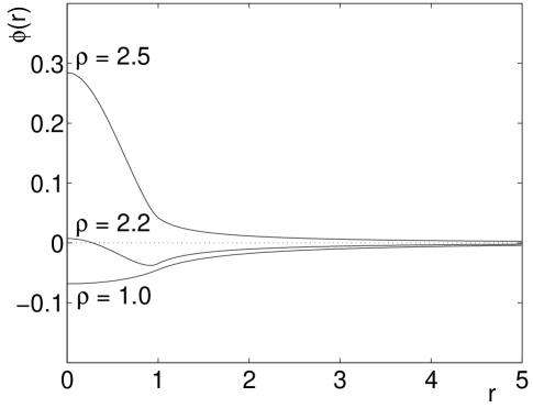
Figure 1: Plots of $\phi$ against $r$ for 3 values of core density, in units where the stellar edge is at $r=1$. For low core density, the deflection is negative, the branes moving apart. For high density, near to the upper mass limit, $\rho_{\rm max}\simeq 2.67$, the deflection becomes entirely positive, and the brane separation is decreased from the unperturbed case.

Figure 2 shows the dependence of the core value of the scalar $\phi$, on the density of the star $\rho_{0}$. We see the linear negative deflections, and then the turn-around to positive deflection for dense stars. The core radion value, $\phi_{0}$, apparently diverges in the positive sense as the upper mass limit is reached, although more detailed numerical analysis would be required to explore this region. We mark on this plot the point where $\rho-3P$ changes sign. In addition the line $\rho-P=0$ is shown, being the point where the dominant energy condition is violated. One sees a tiny positive core deflection just before this, but nothing significant. In the same figure, the right-hand plot shows the core pressure against the density $\rho_{0}$, with the same lines marked. We see to gain a deflection of $\phi_{0}\simeq 1$, one requires extremely large core pressures $P\simeq 40$, compared to the core density $\rho_{0}=2.64$. The data indicates that arbitrarily large $\phi_{0}$ can be reached very close to the upper mass limit, although the form of static matter required to support such a geometry is extremely unrealistic.

         

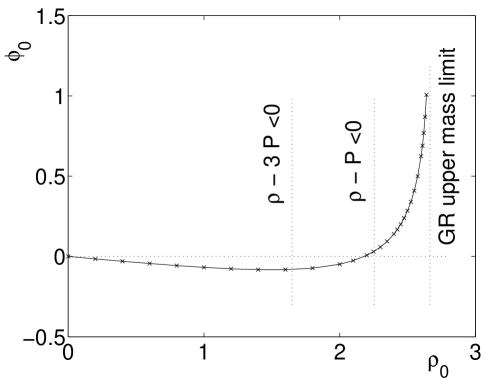
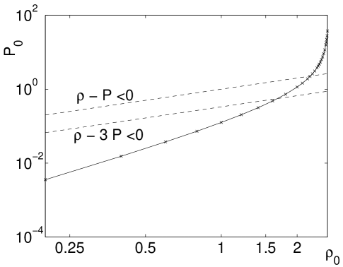
Figure 2: Left-hand frame; Plot of core radion value against stellar density, for incompressible fluid stars with fixed angular radius. The radion appears to diverge in the positive sense close to the upper mass limit. A radion value of $\phi_{0}\simeq 4$ would signal the branes touch. Whilst this will appear to happen very close to the mass limit, we note that $\phi_{0}$ has only just become positive when the dominant energy condition is violated. Thus, it appears for realistic matter, branes will not touch in a static, regular geometry. It is then interesting whether realistic matter may cause localized brane collisions in dynamical situations. Right-hand frame; Plot of core pressure against stellar density. The dominant energy condition is plotted, together with $\rho_{0}-3P_{0}$, whose sign reflects the direction of the brane deflection.

In summary, whilst the scalar radion may become of order $\sim O(1)$ in strong gravity, we find that for static stars, only extreme forms of matter can support configurations where the branes would meet. It is then a very interesting question whether the branes may collide in a dynamical process involving realistic matter. Such dynamics have been studied for Brans-Dicke [56, 57, 58, 59, 60, 61] and it would be interesting to repeat these studies with this scalar-tensor model and realistic matter, to investigate whether there are initial configurations that will collapse to give positive $\phi$ large enough to cause a brane collision, in a region which is outside the formation of an apparent horizon. If such events could occur, it would indicate that the high energy string theory description of colliding branes, might be required to understand low energy, low curvature dynamics in astrophysical processes.

10 Conclusion

We have extended the linearized analysis of the Randall-Sundrum 2 brane compactification to allow the bulk, and induced geometry, to be calculated in the case of low energy strong gravity, with an unperturbed, vacuum negative tension brane. The induced geometry must have low curvature compared to the compactification curvature scale, and the matter energy density must be slowly varying on scales much larger than the compactification length. This is the situation relevant for non-linear gravitation in late time cosmology or astrophysics.

The radion is inhomogeneous in the transverse coordinate for warped compactifications. It therefore can not be included as a homogeneous zero mode, as in usual orbifold reductions. We show how to extend the coordinate systems used in the linear analysis, to the non-linear, low energy case. Firstly we choose a coordinate system analogous to the linear ‘Randall-Sundrum’ gauge. This is Gaussian normal to branes with conformally invariant matter. We then solve the bulk geometry for conformally invariant matter on the positive tension brane, using a formal derivative expansion, which we sum to all orders. General matter is accommodated by introducing a non-linear ‘deflection’ of the positive tension brane with respect to this coordinate system. This deflection is governed by the radion, and is determined to all orders in the bulk derivative expansion. We are then able to understand the radion geometrically, as the proper distance between the two orbifold branes, along a geodesic normal to the vacuum negative tension brane.

Whilst we have applied the method to the 2-brane Randall-Sundrum geometry, the methods can be extended to any warped compactification where the radion is not a simple homogeneous mode. Note also, that we have considered a vacuum negative tension brane, allowing only matter on the positive brane. This is purely for convenience, and can be relaxed more generally using the same techniques.

Having solved the bulk geometry, the effective action on the brane is calculated. To leading order, this yields a scalar-tensor theory with $\omega\propto\Psi/(1-\Psi)$, where $\Psi$ is the scalar depending on the distance between the branes. We have noted that the radion scalar may take values of order $\sim O(1)$ in a strong gravity context, allowing the branes to touch or collide when gravitational fields become strong, and yet curvatures remain small compared to the compactification scale curvature. We have performed calculations for static spherical stars using incompressible fluid matter. For very low density stars, where the response remains linear, the branes are deflected apart. For densities where the gravitational response becomes strong, the brane separation may become reduced. We give evidence that the branes will touch before the stellar upper mass limit is reached, although the dominant energy condition is certainly violated. We find that, as indicated in the linear theory, $\rho-3P$ must become negative to get an appreciable effect. Whilst this does occur for incompressible fluid, it is thought not to for physically reasonable stellar material. Thus we find unrealistic matter is required to create touching branes in a static context. It raises the interesting question of whether realistic matter may allow branes to locally collide in a dynamic context. If this were the case, high energy physics may be required to understand low energy astrophysical processes.

Appendix A: Non-linear Brane Matching Conditions

We now give a detailed derivation of the effective Einstein equations for general matter, that was outlined in section 6. We start by considering the coordinate transformations on the bulk metric (44),

$$z=\bar{z}e^{\phi(\bar{x})},\qquad x^{\mu}=\bar{x}^{\mu}+\xi^{\mu}(\bar{x},\bar{z})$$ (58)

Then preserving the Gaussian normal form of the metric requires that,

$$\bar{\partial_{z}}\xi^{\mu}(\bar{x},\bar{z})=-\bar{z}e^{\phi(\bar{x})}g^{\mu\alpha}(x,z)\bar{\partial}_{\alpha}e^{\phi(\bar{x})}-g^{\mu\alpha}(x,z)g_{\sigma\rho}(x,z)\bar{\partial}_{\alpha}\xi^{\sigma}(\bar{x},\bar{z})\bar{\partial_{z}}\xi^{\rho}(\bar{x},\bar{z})$$ (59)

where $\bar{\partial}_{\alpha},\bar{\partial_{z}}$ are derivatives with respect to $\bar{x}^{\mu}$ and $\bar{z}$. We see that there is the freedom to take $\xi^{\mu}$ to vanish on the brane itself, as boundary data for this differential equation. The metric is then,

$$ds^{2} =\frac{l^{2}}{\bar{z}^{2}}\left[e^{-2\phi(\bar{x})}\bar{g}_{\mu\nu}(\bar{x},\bar{z})d\bar{x}^{\mu}d\bar{x}^{\nu}+N^{2}d\bar{z}^{2}\right]$$

$$\bar{g}_{\mu\nu}(\bar{x},\bar{z}) =g_{\mu\nu}(x,z)+g_{\alpha(\mu}(x,z)\bar{\partial}_{\mu)}\xi^{\alpha}(\bar{x},\bar{z})+g_{\alpha\beta}(x,z)\bar{\partial}_{\mu}\xi^{\alpha}(\bar{x},\bar{z})\bar{\partial}_{\nu}\xi^{\beta}(\bar{x},\bar{z})+\bar{z}^{2}e^{2\phi(\bar{x})}\bar{\partial}_{\mu}\phi(\bar{x})\bar{\partial}_{\nu}\phi(\bar{x})$$

$$N^{2}(\bar{x},\bar{z}) =1+e^{-2\phi(\bar{x})}g_{\alpha\beta}(x,z)(\bar{\partial_{z}}\xi^{\alpha}(\bar{x},\bar{z}))(\bar{\partial_{z}}\xi^{\beta}(\bar{x},\bar{z}))$$ (60)

where we temporarily refrain from expanding the metric $g_{\mu\nu}(x,z)$ in the coordinates $\bar{x},\bar{z}$.

From the linear theory [4, 5] we might expect $\phi$ to be given by an expression similar to $\phi\sim(1/\square)\kappa^{2}_{d}T$. Therefore $\phi\sim\Phi=O(\rho/\epsilon)$ and of course this cannot be assumed to be small. However, we do expect that gradients of $\phi$ are small and use this to perform a gradient expansion of the transformed metric above, as was done for the bulk geometry in section 4. We formalize this with the assumption

$$\|\bar{\partial}_{\alpha}e^{\phi(\bar{z})}\|\sim O(\frac{\rho}{l\sqrt{\epsilon}})\,,\qquad\|\bar{\partial}_{\alpha}\bar{\partial}_{\beta}e^{\phi(\bar{z})}\|\sim O(\rho/l^{2})$$ (61)

which we will see is consistent with the final result. Now considering the off diagonal equation (59), giving $\xi$ in terms of $\phi$, we see the quadratic term in $\xi$ is an order $O(\rho)$ higher. We find to leading order,

$$\bar{\partial_{z}}\xi^{\mu}=-\bar{z}e^{\phi(\bar{x})}{}^{\scriptscriptstyle 0}g^{\mu\alpha}(\bar{x})\bar{\partial}_{\alpha}e^{\phi(\bar{x})}\big{[}1+O(\rho)\big{]}$$ (62)

so that $\bar{\partial_{z}}\xi^{\mu}\sim O(\frac{\rho}{\sqrt{\epsilon}})$. We have decomposed $g_{\mu\nu}(x,z)$ into ${}^{\scriptscriptstyle 0}g_{\mu\nu}(x)$ and $h_{\mu\nu}(x,z)$, and Taylor expanded in $\xi^{\mu}=x^{\mu}-\bar{x}^{\mu}$. Repeating this for (60) we find,

$$\bar{g}_{\mu\nu}(\bar{x},\bar{z}) ={}^{\scriptscriptstyle 0}g_{\mu\nu}(\bar{x})+\big{[}h_{\mu\nu}(\bar{x},\bar{z}e^{\phi(\bar{x})})+\xi^{\alpha}(\bar{x},\bar{z})\bar{\partial}_{\alpha}{}^{\scriptscriptstyle 0}g_{\mu\nu}(\bar{x})+{}^{\scriptscriptstyle 0}g_{\alpha(\mu} (\bar{x})\bar{\partial}_{\nu)}\xi^{\alpha}(\bar{x},\bar{z})$$

$$\qquad O(1)\qquad\qquad\qquad\qquad O(\rho) +\bar{z}^{2}(\bar{\partial}_{\mu}e^{\phi(\bar{x})})(\bar{\partial}_{\nu}e^{\phi(\bar{x})})\big{]}+O(\rho^{2})$$

$$N^{2} =1+e^{-2\phi(\bar{x})}{}^{\scriptscriptstyle 0}g_{\alpha\beta}(\bar{x})\bar{\partial_{z}}\xi^{\alpha}(\bar{x},\bar{z})\bar{\partial_{z}}\xi^{\beta}(\bar{x},\bar{z})+O(\rho^{2})$$

$$\quad O(1)\qquad\qquad\qquad O(\rho)$$ (63)

Whilst we may Taylor expand $h_{\mu\nu}(\bar{x}+\xi,\bar{z}e^{\phi})$ in $\xi$, as $\xi$ is small $\sim O(\frac{\rho l}{\sqrt{\epsilon}})$, $\phi$ is not small and may be of order one. However, we know the explicit $z$ dependence of $h_{\mu\nu}$ for each order in the derivative expansion and therefore we may simply evaluate $h_{\mu\nu}$ at $z=\bar{z}e^{\phi}$, rather than having to perform a Taylor expansion. Thus,

$$h_{\mu\nu}(\bar{x},\bar{z}e^{\phi(\bar{x})})=\left(B_{0}-\frac{1}{d-2}\bar{z}^{2}e^{2\phi(\bar{x})}+A_{0}\bar{z}^{d}e^{d\phi(\bar{x})}\right){}^{\scriptscriptstyle 0}G_{\mu\nu}(\bar{x})+O(l^{4}{}^{\scriptscriptstyle 0}\square{}^{\scriptscriptstyle 0}G_{\mu\nu})$$ (64)

As in the conformal matter case, $h_{\mu\nu}$ will not contribute to leading order in the induced metric, but will do in the localized stress energy. The induced metric on the brane at $\bar{z}=\bar{z}_{1}$ is simply,

$${}^{\scriptscriptstyle I}g_{\mu\nu}(\bar{x})=\frac{l^{2}}{\bar{z}_{1}^{2}}e^{-2\phi(\bar{x})}\bar{g}_{\mu\nu}(\bar{x},\bar{z}_{1})=\frac{l^{2}}{\bar{z}_{1}^{2}}e^{-2\phi(x)}{}^{\scriptscriptstyle 0}g_{\mu\nu}(x)+O(\rho)$$ (65)

where we use the fact that $\bar{x}^{\alpha}=x^{\alpha}$ on the brane. The $O(\rho)$ terms, which involve $h_{\mu\nu}$, are not relevant if one is only working to leading order in the derivative expansion, and their absence makes the following computations considerably simpler.

We calculate the stress energy, $\kappa^{2}_{d+1}{}^{\scriptscriptstyle I}T_{\mu\nu}(\bar{x})=\kappa^{2}_{d+1}\sigma{}^{\scriptscriptstyle I}g_{\mu\nu}+2\left[K_{\mu\nu}-K{}^{\scriptscriptstyle I}g_{\mu\nu}\right]_{\bar{z}=\bar{z}_{1}}$, as,

$$\kappa^{2}_{d+1}{}^{\scriptscriptstyle I}T_{\mu\nu}(x) =-\frac{l}{\bar{z}_{1}}e^{-2\phi(x)}(\bar{\partial_{z}}h_{\mu\nu}(\bar{x},\bar{z}e^{\phi(\bar{x})}))\mid_{\bar{z}=\bar{z}_{1}}+2l{\cal A}_{\mu\nu}[\phi(x)]+O(\rho^{2}/l)$$

$${\cal A}_{\mu\nu}[\phi(x)] =\left({}^{\scriptscriptstyle I}\nabla_{\mu}{}^{\scriptscriptstyle I}\nabla_{\nu}-{}^{\scriptscriptstyle I}g_{\mu\nu}{}^{\scriptscriptstyle I}\square\right)\phi(x)-({}^{\scriptscriptstyle I}\nabla_{\mu}\phi(x))({}^{\scriptscriptstyle I}\nabla_{\nu}\phi(x))-\frac{d-3}{2}({}^{\scriptscriptstyle I}\nabla\phi(x))^{2}{}^{\scriptscriptstyle I}g_{\mu\nu}$$ (66)

where ${}^{\scriptscriptstyle I}\nabla$ is the covariant derivative of the induced brane metric ${}^{\scriptscriptstyle I}g_{\mu\nu}(x)$ and,

$$\bar{\partial_{z}}h_{\mu\nu}(\bar{x},\bar{z}e^{\phi(\bar{x})}))\mid_{\bar{z}=\bar{z}_{1}}=\left(-\frac{2}{d-2}\bar{z}_{1}e^{2\phi(\bar{x})}+A_{0}\,d\,\bar{z}_{1}^{d-1}e^{d\phi(\bar{x})}\right){}^{\scriptscriptstyle 0}G_{\mu\nu}(\bar{x})+O(l^{3}{}^{\scriptscriptstyle 0}\square{}^{\scriptscriptstyle 0}G)$$ (67)

As in the linear analysis, the trace of (66) determines $\phi(x)$ as,

$${}^{\scriptscriptstyle I}g^{\mu\nu}(\bar{x})(\bar{\partial_{z}}h_{\mu\nu}(\bar{x},\bar{z}e^{\phi(\bar{x})}))=\frac{\bar{z}^{2}}{l^{2}}e^{2\phi(\bar{x})}\bar{\partial_{z}}\left({}^{\scriptscriptstyle 0}g^{\mu\nu}(\bar{x})h_{\mu\nu}(\bar{x},\bar{z}e^{\phi(\bar{x})})\right)+O(\rho^{2})=O(\rho^{2})$$ (68)

and $h_{\mu\nu}$ is traceless with respect to ${}^{\scriptscriptstyle 0}g_{\mu\nu}$. This then determines the location of the brane in the $z$ coordinate system by specifying that the radion $\phi$ must obey,

$${}^{\scriptscriptstyle I}\square\phi(x)+\frac{d-2}{2}({}^{\scriptscriptstyle I}\nabla\phi(x))^{2}=-\frac{1}{2(d-1)}\frac{\kappa^{2}_{d+1}}{l}{}^{\scriptscriptstyle I}T^{\alpha}{}_{\alpha}(x)+O(\rho^{2}/l^{2})$$ (69)

This result is interesting as it is exact to all orders in the derivative expansion. From (65) the induced metric is simply a conformal transformation of the zero mode metric ${}^{\scriptscriptstyle 0}g_{\mu\nu}$ by $e^{2\phi(x)}$, to leading order, resulting in an induced Einstein tensor,

$${}^{\scriptscriptstyle I}G_{\mu\nu}(x)={}^{\scriptscriptstyle 0}G_{\mu\nu}(x)+(d-2){\cal A}_{\mu\nu}[\phi(x)]+O(\max(l^{2}{}^{\scriptscriptstyle 0}\square{}^{\scriptscriptstyle 0}G_{\mu\nu},\rho^{2}/l^{2})$$ (70)

where ${}^{\scriptscriptstyle 0}\square{}^{\scriptscriptstyle 0}G_{\mu\nu}$ terms appear if one works to higher order in the derivative expansion including the terms $O(\rho)$ in (65). All that remains is to solve (66) for ${}^{\scriptscriptstyle 0}G_{\mu\nu}$, and substitute into (70) to derive the induced Einstein equations on the brane, to leading order in the derivative expansion,

$${}^{\scriptscriptstyle I}G_{\mu\nu}(x)=\kappa^{2}_{d}\frac{1}{1-\Omega[\phi(x)]} {}^{\scriptscriptstyle I}T_{\mu\nu}(x)-(d-2)\frac{\Omega[\phi(x)]}{1-\Omega[\phi(x)]}{\cal A}_{\mu\nu}[\phi(x)]+O(\max(l^{2}{}^{\scriptscriptstyle I}\square\kappa^{2}_{d}{}^{\scriptscriptstyle I}T_{\mu\nu},\rho^{2}/l^{2}))$$

$$\Omega[\phi(x)] =\left(\frac{\bar{z}_{1}e^{\phi(x)}}{z_{2}}\right)^{d-2},\qquad\kappa^{2}_{d}=\frac{d-2}{2}\frac{\kappa^{2}_{d+1}}{l}$$ (71)

which together with the equation (69) determining $\phi(x)$, fully specifies the induced Einstein equations, up to corrections $O(l^{2}{}^{\scriptscriptstyle 0}\square{}^{\scriptscriptstyle 0}G_{\mu\nu})$ from sub-leading ‘Kaluza-Klein’ terms. Tracing these equations, and using the equation for $\phi$, one obtains,

$${}^{\scriptscriptstyle I}R=-\frac{\kappa^{2}_{d+1}}{l}{}^{\scriptscriptstyle I}T$$ (72)

which is true to all orders in the derivative expansion, the corrections being traceless.

The sub-leading terms have a complicated form when written in the induced metric Laplacian, rather than ${}^{\scriptscriptstyle 0}\square$, which is the Laplacian of ${}^{\scriptscriptstyle 0}g_{\mu\nu}$. However, of course these terms can be evaluated if required, and are briefly discussed in the following Appendix B.

Appendix B: Sub-leading Non-Local Terms

We now consider the form that sub-leading non-local terms will take in the effective Einstein equations. Note that such corrections are only of interest when $\Phi<<1$, as otherwise they are of order $O(\rho^{2})$, comparable with the other set of bulk corrections we have ignored.

In the conformally invariant case we have formally summed the derivative expansion (39). This is considerably more complicated to do in the non-conformal case, the primary reason being that $h_{\mu\nu}$ no longer vanishes on the brane, when it is not located at constant $z$ as in the conformal case. Whilst the induced metric in the conformal case is simply ${}^{\scriptscriptstyle I}g_{\mu\nu}=(l^{2}/z_{1}^{2}){}^{\scriptscriptstyle 0}g_{\mu\nu}$, in the non-conformal case,

$${}^{\scriptscriptstyle I}g_{\mu\nu}(\bar{x})=\frac{l^{2}}{\bar{z}_{1}^{2}}e^{-2\phi(x)}\left({}^{\scriptscriptstyle 0}g_{\mu\nu}(x)+\left[h_{\mu\nu}(x,\bar{z}_{1}e^{\phi(x)})+\bar{z}_{1}^{2}(\partial_{\mu}e^{\phi(x)})(\partial_{\nu}e^{\phi(x)})\right]\right)+O(\rho^{2})$$ (73)

which is presented above in equation (65) only to leading order as sub-leading terms were not considered. One can rewrite this as,

$$\frac{\bar{z}_{1}^{2}}{l^{2}}e^{+2\phi(x)}{}^{\scriptscriptstyle I}g_{\mu\nu}(x)={}^{\scriptscriptstyle 0}g_{\mu\nu}(x)+\left[h_{\mu\nu}(x,\bar{z}_{1}e^{\phi(x)})+\bar{z}_{1}^{2}({}^{\scriptscriptstyle 0}\nabla_{\mu}e^{\phi(x)})({}^{\scriptscriptstyle 0}\nabla_{\nu}e^{\phi(x)})\right]+O(\rho^{2})$$ (74)

and then calculate the Einstein curvature of both sides perturbatively using ${}^{\scriptscriptstyle I}g_{\mu\nu}$ as the background metric on the left-hand side, and ${}^{\scriptscriptstyle 0}g_{\mu\nu}$ on the right, giving,

$${}^{\scriptscriptstyle I}G_{\mu\nu}(x)-(d-2){\cal A}_{\mu\nu}[\phi(x)]={}^{\scriptscriptstyle 0}G_{\mu\nu}(x)-\frac{1}{2}{}^{\scriptscriptstyle 0}\square h_{\mu\nu}(x,\bar{z}e^{\phi(x)})+O(\rho^{2}/l^{2})$$ (75)

where the term $\bar{z}_{1}^{2}({}^{\scriptscriptstyle 0}\nabla_{\mu}e^{\phi})({}^{\scriptscriptstyle 0}\nabla_{\nu}e^{\phi})$ from the metric perturbation on the right hand side of (74) in fact contributes only to $O(\rho^{2}/l^{2})$. A subtlety in this calculation is that ${}^{\scriptscriptstyle 0}\nabla^{\alpha}h_{\alpha\mu}(x,\bar{z}e^{\phi})$ is not zero due to the implicit $e^{\phi}$ dependence. However, one finds that,

$${}^{\scriptscriptstyle 0}\nabla^{\alpha}h_{\alpha\mu}(x,\bar{z}e^{\phi})=\left({}^{\scriptscriptstyle 0}\nabla^{\alpha}\phi\right)\bar{z}\partial_{\bar{z}}h_{\alpha\mu}(x,\bar{z}e^{\phi})\sim O((L\rho)(\frac{\rho}{lL}))=O(\rho^{2}/l)$$ (76)

and so these terms can be ignored. Indeed, if $\Phi\sim 1$, then $\|\phi\|\sim 1$ but the first sub-leading term is of order $O(\rho^{2})$ and is not useful without calculating the other $O(\rho^{2})$ corrections. If $\Phi<<1$, then similarly $\|\phi\|<<1$. One finds that whilst it is important to consider the $\phi$ dependence in the leading term of the derivative expansion of $h_{\mu\nu}$, which results in the recovery of the scalar-tensor behavior, for the sub-leading terms, $\phi$ corrections are in fact negligible. Remembering we are considering the case $\|\phi\|<<1$, consider the two contributions,

$$\phi{}^{\scriptscriptstyle 0}G_{\mu\nu} \sim(L^{2}\rho)(\rho/l^{2})$$

$$\phi{}^{\scriptscriptstyle 0}\square{}^{\scriptscriptstyle 0}G_{\mu\nu} \sim(L^{2}\rho)(\frac{1}{L^{2}})(\rho/l^{2})=O(\rho^{2}/l^{2})$$ (77)

Whilst the first term, which could be found in the leading term of the expansion of $h_{\mu\nu}$ is still relevant in the Einstein equations, the second term, found in the first sub-leading correction, is not as it is of order $O(\rho^{2}/l^{2})$.

In order to write the effective Einstein equations as done in equation (71), one must eliminate ${}^{\scriptscriptstyle 0}G_{\mu\nu}$ between (66) and (75). To leading order in the derivative expansion this is trivial as (75) is inverted to solve for ${}^{\scriptscriptstyle 0}G_{\mu\nu}$ simply by rearrangement. However to sub-leading order this is a slightly more tricky procedure in general, as one must invert the derivative expansion. Of course this can be done if such terms are required, although we refrain from calculating them here. The final step is then to convert ${}^{\scriptscriptstyle 0}G_{\mu\nu}$ to ${}^{\scriptscriptstyle I}G_{\mu\nu}$ and ${}^{\scriptscriptstyle 0}\square$ to ${}^{\scriptscriptstyle I}\square$.

References

- [1] L. Randall and R. Sundrum: A large mass hierarchy from a small extra dimension. Phys. Rev. Lett. 83 (1999) 3370–3373, hep-ph/9905221.
- [2] L. Randall and R. Sundrum: An alternative to compactification. Phys. Rev. Lett. 83 (1999) 4690, hep-th/9906064.
- [3] J. Lykken and L. Randall: The shape of gravity. JHEP 06 (2000) 014, hep-th/9908076.
- [4] J. Garriga and T. Tanaka: Gravity in the brane-world. Phys. Rev. Lett. 84 (2000) 2778–2781, hep-th/9911055.
- [5] S. Giddings, E. Katz and L. Randall: Linearized gravity in brane backgrounds. JHEP 03 (2000) 023, hep-th/0002091.
- [6] T. Tanaka: Asymptotic behavior of perturbations in Randall-Sundrum brane-world. Prog. Theor. Phys. 104 (2000) 545–554, hep-ph/0006052.
- [7] M. Sasaki, T. Shiromizu and K. Maeda: Gravity, stability and energy conservation on the Randall- Sundrum brane-world. Phys. Rev. D62 (2000) 024008, hep-th/9912233.
- [8] R. Emparan, G. Horowitz and R. Myers: Exact description of black holes on branes. JHEP 01 (2000) 007, hep-th/9911043.
- [9] R. Emparan: Exact gravitational shockwaves and Planckian scattering on branes. Phys. Rev. D64 (2001) 024025, hep-th/0104009.
- [10] H. Kudoh and T. Tanaka: Second order perturbations in the Randall-Sundrum infinite brane-world model (2001). Preprint hep-th/0104049.
- [11] I. Giannakis and H. Ren: Recovery of the Schwarzschild metric in theories with localized gravity beyond linear order. Phys. Rev. D63 (2001) 024001, hep-th/0007053.
- [12] T. Wiseman: Relativistic Stars in Randall-Sundrum Gravity (2001). Preprint hep-th/0111057.
- [13] R. Gregory and A. Padilla: Nested braneworlds and strong brane gravity (2001). Preprint hep-th/0104262.
- [14] W. Goldberger and M. Wise: Modulus stabilization with bulk fields. Phys. Rev. Lett. 83 (1999) 4922–4925, hep-ph/9907447.
- [15] W. Goldberger and M. Wise: Phenomenology of a stabilized modulus. Phys. Lett. B475 (2000) 275–279, hep-ph/9911457.
- [16] W. Goldberger and M. Wise: Bulk fields in the Randall-Sundrum compactification scenario. Phys. Rev. D60 (1999) 107505, hep-ph/9907218.
- [17] C. Csaki, M. Graesser, L. Randall and J. Terning: Cosmology of brane models with radion stabilization. Phys. Rev. D62 (2000) 045015, hep-ph/9911406.
- [18] T. Tanaka and X. Montes: Gravity in the brane-world for two-branes model with stabilized modulus. Nucl. Phys. B582 (2000) 259–276, hep-th/0001092.
- [19] S. Mukohyama and L. Kofman: Brane Gravity at Low Energy (2001). Preprint hep-th/0112115.
- [20] H. Kudoh and T. Tanaka: Second order perturbations in the radius stabilized Randall-Sundrum two branes model (2001). Preprint hep-th/0112013.
- [21] P. Steinhardt and N. Turok: Cosmic evolution in a cyclic universe (2001), hep-th/0111098.
- [22] P. Steinhardt and N. Turok: A cyclic model of the universe (2001), hep-th/0111030.
- [23] P. Horava and E. Witten: Eleven-Dimensional Supergravity on a Manifold with Boundary. Nucl. Phys. B475 (1996) 94–114, hep-th/9603142.
- [24] Z. Lalak, A. Lukas and B. Ovrut: Soliton solutions of M-theory on an orbifold. Phys. Lett. B425 (1998) 59–70, hep-th/9709214.
- [25] A. Lukas, B. Ovrut and D. Waldram: On the four-dimensional effective action of strongly coupled heterotic string theory. Nucl. Phys. B532 (1998) 43–82, hep-th/9710208.
- [26] A. Lukas, B. Ovrut, K. Stelle and D. Waldram: Heterotic M-theory in five dimensions. Nucl. Phys. B552 (1999) 246–290, hep-th/9806051.
- [27] A. Lukas, B. Ovrut and D. Waldram: The ten-dimensional effective action of strongly coupled heterotic string theory. Nucl. Phys. B540 (1999) 230–246, hep-th/9801087.
- [28] A. Lukas, B. Ovrut and D. Waldram: Boundary inflation. Phys. Rev. D61 (2000) 023506, hep-th/9902071.
- [29] C. Charmousis, R. Gregory and V. Rubakov A.: Wave function of the radion in a brane world. Phys. Rev. D62 (2000) 067505, hep-th/9912160.
- [30] U. Gen and M. Sasaki: Radion on the de Sitter brane (2000), gr-qc/0011078.
- [31] Z. Chacko and P. Fox: Wave function of the radion in the dS and AdS brane worlds. Phys. Rev. D64 (2001) 024015, hep-th/0102023.
- [32] I. Kogan, S. Mouslopoulos, A. Papazoglou and L. Pilo: Radion in multibrane world (2001), hep-th/0105255.
- [33] T. Chiba: Scalar-tensor gravity in two 3-brane system. Phys. Rev. D62 (2000) 021502, gr-qc/0001029.
- [34] P. Binetruy, C. Deffayet, U. Ellwanger and D. Langlois: Brane cosmological evolution in a bulk with cosmological constant. Phys. Lett. B477 (2000) 285, hep-th/9910219.
- [35] P. Binetruy, C. Deffayet and D. Langlois: The radion in brane cosmology. Nucl. Phys. B615 (2001) 219–236, hep-th/0101234.
- [36] C. Germani and R. Maartens: Stars in the braneworld (2001). Preprint hep-th/0107011.
- [37] N. Deruelle: Stars on branes: The view from the brane (2001), gr-qc/0111065.
- [38] T. Shiromizu, K. Maeda and M. Sasaki: The Einstein equations on the 3-brane world. Phys. Rev. D62 (2000) 024012, gr-qc/9910076.
- [39] D. Brecher and M. Perry: Ricci-flat branes. Nucl. Phys. B566 (2000) 151, hep-th/9908018.
- [40] W. Israel: Singular hypersurfaces and thin shells in general relativity. Nuovo Cim. B44S10 (1966) 1.
- [41] S. Mukohyama: Brane gravity, higher derivative terms and non-locality (2001). Preprint hep-th/0112205.
- [42] C. Will: The confrontation between general relativity and experiment. Living Rev. Rel. 4 (2001) 4, gr-qc/0103036.
- [43] D. Ida: Brane-world cosmology. JHEP 09 (2000) 014, gr-qc/9912002.
- [44] S. Mukohyama: Brane-world solutions, standard cosmology, and dark radiation. Phys. Lett. B473 (2000) 241–245, hep-th/9911165.
- [45] D. Vollick: Cosmology on a three-brane. Class. Quant. Grav. 18 (2001) 1–10, hep-th/9911181.
- [46] P. Kraus: Dynamics of anti-de Sitter domain walls. JHEP 12 (1999) 011, hep-th/9910149.
- [47] A. Chamblin and H. Reall: Dynamic dilatonic domain walls. Nucl. Phys. B562 (1999) 133, hep-th/9903225.
- [48] P. Bowcock, C. Charmousis and R. Gregory: General brane cosmologies and their global spacetime structure. Class. Quant. Grav. 17 (2000) 4745–4764, hep-th/0007177.
- [49] S. Mukohyama, T. Shiromizu and K. Maeda: Global structure of exact cosmological solutions in the brane world. Phys. Rev. D62 (2000) 024028, hep-th/9912287.
- [50] T. Harada: Stability analysis of spherically symmetric star in scalar- tensor theories of gravity. Prog. Theor. Phys. 98 (1997) 359–379, gr-qc/9706014.
- [51] T. Harada: Neutron stars in scalar-tensor theories of gravity and catastrophe theory. Phys. Rev. D57 (1998) 4802–4811, gr-qc/9801049.
- [52] T. Damour and G. Esposito-Farese: Nonperturbative strong field effects in tensor - scalar theories of gravitation. Phys. Rev. Lett. 70 (1993) 2220–2223.
- [53] T. Damour and G. Esposito-Farese: Tensor-scalar gravity and binary-pulsar experiments. Phys. Rev. D54 (1996) 1474–1491, gr-qc/9602056.
- [54] J. Novak: Neutron star transition to strong-scalar-field state in tensor-scalar gravity. Phys. Rev. D58 (1998) 064019, gr-qc/9806022.
- [55] T. Tsuchida, G. Kawamura and K. Watanabe: A maximum mass-to-size ratio in scalar-tensor theories of gravity. Prog. Theor. Phys. 100 (1998) 291–313, gr-qc/9802049.
- [56] M. Shibata, K. Nakao and T. Nakamura: Scalar type gravitational wave emission from gravitational collapse in Brans-Dicke theory: Detectability by a laser interferometer. Phys. Rev. D50 (1994) 7304–7317.
- [57] M. Scheel, S. Shapiro and S. Teukolsky: Collapse to black holes in Brans-Dicke theory. 1. Horizon boundary conditions for dynamical space-times. Phys. Rev. D51 (1995) 4208–4235, gr-qc/9411025.
- [58] M. Scheel, S. Shapiro and S. Teukolsky: Collapse to black holes in Brans-Dicke theory. 2. Comparison with general relativity. Phys. Rev. D51 (1995) 4236–4249, gr-qc/9411026.
- [59] T. Harada, T. Chiba, K. Nakao and T. Nakamura: Scalar gravitational wave from Oppenheimer-Snyder collapse in scalar-tensor theories of gravity. Phys. Rev. D55 (1997) 2024–2037, gr-qc/9611031.
- [60] J. Balakrishna and H. Shinkai: Dynamical evolution of boson stars in Brans-Dicke theory. Phys. Rev. D58 (1998) 044016, gr-qc/9712065.
- [61] J. Kerimo and D. Kalligas: Gravitational collapse of collisionless matter in scalar tensor theories: Scalar waves and black hole formation. Phys. Rev. D58 (1998) 104002.