hep-th/0112221 UT-981

Comments on D-branes in Kazama-Suzuki models

and Landau-Ginzburg theories

Masatoshi Nozaki
nozaki@hep-th.phys.s.u-tokyo.ac.jp

Department of Physics, Faculty of Science
University of Tokyo
Bunkyo-ku, Hongo 7-3-1, Tokyo 113-0033, Japan

We study D-branes in Kazama-Suzuki models by means of the boundary state description. We can identify the boundary states of Kazama-Suzuki models with the solitons in ${\cal N}=2$ Landau-Ginzburg theories. We also propose a geometrical interpretation of the boundary states in Kazama-Suzuki models.

1 Introduction

In considering a string compactification, one of the most important subjects is the physics near a singularity. Some of cycles vanish near the singularity and various nonperturbative phenomena take place [1, 2]. To reveal the whole picture of string theory, we should further investigate this subject. In particular, among the many recent studies of string compactification on singular Calabi-Yau manifolds [3, 4, 5, 6, 7, 8, 9, 10, 11], Gukov, Vafa and Witten have argued an interesting proposal [5]. They consider a two dimensional field theory with four supercharges constructed in Type IIA string theory on a Calabi-Yau four-fold with an isolated singularity that flows into a non-trivial space-time superconformal theory at the infrared fixed point. Near an isolated singularity, nonperturbative physics often generates massless chiral supermultiplets and a superpotential. Then they proposed that from the non-compact Calabi-Yau four-folds that are ALE fibrations with appropriate RR-fluxes, one can obtain the perturbed Kazama-Suzuki models [12] at level one that have Landau-Ginzburg descriptions. In fact, by analyzing the vacuum and soliton structure of each theory, they have found one to one correspondence between the BPS D-branes wrapped on a 4-cycle in a non-compact Calabi-Yau four-fold and the BPS domain walls in the Landau-Ginzburg theory that flows to a Kazama-Suzuki model.

Now we would like to discuss what objects in the Kazama-Suzuki model correspond to the solitons in the Landau-Ginzburg theory. As far as the closed string physics is concerned, there have been a lot of works to find the correspondence between the Kazama-Suzuki models and the Landau-Ginzburg theories [13, 14, 15, 16, 17, 18, 19]. In particular, it was shown that the chiral ring of the coset model at level one is isomorphic to the de Rham cohomology ring of Grassmannian. It has also been argued that the ring is described in terms of the polynomial ring of Landau-Ginzburg theory.

We will consider the correspondence from the viewpoint of the models that have a boundary on the world-sheet. Then there are so-called “boundary states” in such models that should correspond to D-branes wrapped on certain cycles. Now our question is what the boundary states in the Kazama-Suzuki models describe. (Some works have been done for the case of the ${\cal N}=2$ minimal models [20, 21, 22, 23, 24] and for the Kazama-Suzuki models [25].) We will show that the boundary states in the Kazama-Suzuki models are identified with the solitons in the Landau-Ginzburg theories. Therefore we propose that the boundary states in the Kazama-Suzuki models can be thought of as BPS D4-branes wrapped on the 4-cycles in a non-compact Calabi-Yau four-fold with an appropriate RR-flux, or at least they describe a sub-sector of the BPS D-branes that sufficiently capture the information of the singularity. Our result is indeed a first step to understand this relation and the further investigations are required.

This paper is organized as follows. We first give a brief review of the Kazama-Suzuki model in Section 2 and we explicitly show the construction of the boundary states in the Kazama-Suzuki model which indeed satisfy the Cardy condition [26]. In Section 3, we summarize the basic facts about the Landau-Ginzburg theory. In particular, we review how to derive the soliton structure of the theory which should correspond to the boundary states in the Kazama-Suzuki model. Then we find the correspondence between the boundary states in Kazama-Suzuki model and the solitons in Landau-Ginzburg theory in Section 4. We give two examples there and discuss the geometrical interpretation of the boundary states. Finally in section 5, we discuss some of our results and unsolved problems. In the appendix, we summarize the characters and the S-matrices used in this paper.

2 Boundary states in Kazama-Suzuki models

2.1 Review of the Kazama-Suzuki models

The Kazama-Suzuki coset models $G/H$ are the large class of solvable two dimensional conformal field theories which possess an ${\cal N}=2$ superconformal symmetry [12]. These models were constructed by first applying so-called coset ($G/H$) construction to super-Kac-Moody algebra of group $G$ to obtain ${\cal N}=1$ superconformal algebra. Then the conditions under which the ${\cal N}=1$ models actually possess ${\cal N}=2$ superconformal symmetry were examined. The result is simple; the condition is that the coset manifold $G/H$ is Kählerian. By way of notation, let $r$ be the rank of $G$, and $g_{G}$ and $g_{H}$ are the dual Coxeter numbers of $G$ and $H$, respectively. Then the $G/H$ superconformal model can be decomposed as

$$\frac{\widehat{G}_{k}\times\widehat{SO}(2d)_{1}}{\widehat{H}_{k+g_{G}-g_{H}}}~{},$$ (2.1)

where $d={1\over 2}{\rm dim}(G/H)$ and the $\widehat{SO}(2d)_{1}$ factor arises from the fermions. Among the Kählerian models, we consider the special class of the coset spaces, so-called simply laced, level one, hermitian symmetric spaces (SLOHSS). In particular, the explicit model we would like to investigate here is

$$\frac{\widehat{SU}(n+k)_{1}\times\widehat{SO}(2nk)_{1}}{\widehat{SU}(n)_{k+1}\times\widehat{SU}(k)_{n+1}\times\widehat{U}(1)_{kn(k+n)(k+n+1)}}\cong\frac{\widehat{SU}(n+1)_{k}\times\widehat{SO}(2n)_{1}}{\widehat{SU}(n)_{k+1}\times\widehat{U}(1)_{n(n+1)(k+n+1)}}~{},$$ (2.2)

where the left and right models are equivalent by the level-rank duality [12, 13, 27, 28]. The central charge of this Kazama-Suzuki model is $c={3nk\over k+n+1}$. From now on, we will consider only the right hand of this model, namely “${\bf C}{\bf P}^{n}$ model at level $k$”.

The primary states of this ${\cal N}=2$ coset model are represented as those of the Kac-Moody algebra of group $G$, $H=H_{0}\times U(1)$ and $SO(2d)$. At first, the highest weights of the Lie algebra associated with $G$ are labeled by

$$\Lambda=\sum_{i=1}^{r}\ell_{i}\omega_{i}~{},$$ (2.3)

where $\omega_{i}$ denotes the fundamental weight and the $\ell_{i}$’s are all non-negative integers satisfying $\sum\ell_{i}\leq k$. From now on, we denote the weight as the component form $\Lambda=(\ell_{1},\ldots,\ell_{r})$. The highest weights of $SO(2d)$ at level 1 are represented by

$$s=0,2,1,-1~{},$$ (2.4)

which correspond to besic ($s=0$), vector ($s=2$), spinor ($s=1$) and cospinor ($s=-1$) representations, respectively. Then the basis of the Hilbert space of ${\cal N}=2$ coset model can be obtained by decomposing ${\cal H}^{\Lambda}\otimes{\cal H}^{s}$ into the irreducible representations of the group $H$, i.e.

$${\cal H}^{\Lambda}\otimes{\cal H}^{s}=\sum_{\lambda,m}{\cal H}^{\Lambda,s}_{\lambda,m}\otimes{\cal H}^{\lambda,m}~{},$$ (2.5)

where the $(\lambda,m)$ label the highest weight of $H=H_{0}\times U(1)$. Thus the highest weight state is denoted by ${|\Lambda,\lambda,m,s\rangle}$.

However not all sub-sectors of the Hilbert space ${\cal H}_{\lambda,m}^{\Lambda,s}$ are independent. There is a special relation among them. At first, the characters of the ${\cal N}=2$ coset model do not vanish if the labels satisfy the following selection rule [30, 13]

$$\frac{|\Lambda|}{n+1}-\frac{|\lambda|}{n}+{m\over n(n+1)}-{s\over 2}=0\quad\mbox{mod}\;1~{},$$ (2.6)

where $|\Lambda|=\sum_{i=1}^{r}i\ell_{i}$ denotes the number of boxes in the Young tableau corresponding to the weight $\Lambda$ of $SU(n+1)_{k}$ and $|\lambda|$ denotes the number of boxes corresponding to the weight $\lambda$ of $SU(n)_{k+1}$ . There is also another constraint, i.e. the field identification. The outer-automorphism of the extended Dynkin diagrams of $G$ and $H$ will force certain field identifications. Now let us consider the model (2.2). We set the generators of outer-automorphism of ($\widehat{SU}(n+1)_{k},\widehat{SU}(n)_{k+1},\widehat{U}(1),\widehat{SO}(2d)_{1}$) as $(A,a,h,v)$, where $h=k+n+1$ and $v$ denotes the vector. Then the labels $(\Lambda,\lambda,m,s)$ are identified under the action of ${\cal J}=(A,a,h,v)$,

$$(\Lambda,\lambda,m,s)\sim{\cal J}(\Lambda,\lambda,m,s)\equiv(A(\Lambda),a(\lambda),m+h,s+v)~{}.$$ (2.7)

The order of this generator in the model (2.2) is $n(n+1)$. In general, there are some fixed points among the ${\cal H}_{\lambda,m}^{\Lambda,s}$ space under the field identifications [29]. However, for simply laced $G$ at level one there are no fixed point problems and this is indeed the model we discuss in this paper.

In the case of the model (2.2), the conformal dimension $h$ and the $U(1)$ charge $q$ of the primary state $(\Lambda,\lambda,m,s)$ is

$$h = {1\over 2(k+n+1)}\left[\Lambda(\Lambda+2\rho_{G})-\lambda(\lambda+2\rho_{H})-{m^{2}\over n(n+1)}\right]+g(s)\quad\mbox{mod}\;{\bf Z}~{},$$

$$q = f(s)-{m\over n+k+1}\quad\mbox{mod}\;2{\bf Z}~{},$$ (2.8)

where

$$g(s) = (0,{1\over 2},{d\over 8},{d\over 8})\quad{\rm for}\quad s=(0,2,1,-1)~{},$$ (2.9)

$$f(s) = (0,1,{d\over 2},{d\over 2}-1)\quad{\rm for}\quad s=(0,2,1,-1)\quad{\rm of}\quad\widehat{SO}(2d)_{1}~{},$$ (2.10)

and $\rho_{G}$ and $\rho_{H}$ are the Weyl vectors of $G$ and $H$, respectively.

The chiral primaries ($h=q/2$ mod ${\bf Z}$) are labeled by [27]

$$\widehat{SU}(n+1)_{k} : \Lambda=(\ell_{1},\ell_{2},\cdots,\ell_{n})~{},$$

$$\widehat{SU}(n)_{k+1} : \lambda=(\ell_{1},\ell_{2},\cdots,\ell_{n-1})~{},$$ (2.11)

$$\widehat{U}(1)_{n(n+1)(n+k+1)} : m=\sum_{i=1}^{n}i\ell_{i}~{},$$

and the number of the chiral primaries is $\left(n+k\atop k\right)$.

2.2 Boundary states in Kazama-Suzuki model

As is well known, D-branes can be described either in terms of boundary conditions of open strings or as boundary states in the closed string channel. Boundary conditions for ${\cal N}=2$ superconformal field theory were investigated in [31] and explicit boundary conditions for Kazama-Suzuki model was given in [32]. Two types of boundary conditions are possible for ${\cal N}=2$ superconformal currents and are called as the A-type and the B-type conditions. In the closed string channel, these conditions on the boundary $z=\bar{z}$ of world-sheet are represented as

A-type boundary condition:

$$(T-{\bar{T}}){|B;\eta\rangle}=0~{},\quad(G^{\pm}-i\eta{\bar{G}}^{\mp}){|B;\eta\rangle}=0~{},\quad(J-{\bar{J}}){|B;\eta\rangle}=0~{},$$ (2.12)

B-type boundary condition:

$$(T-{\bar{T}}){|B;\eta\rangle}=0~{},\quad(G^{\pm}-i\eta{\bar{G}}^{\pm}){|B;\eta\rangle}=0~{},\quad(J+{\bar{J}}){|B;\eta\rangle}=0~{},$$ (2.13)

where $\eta=\pm 1$ is the different choice of the spin structure. From now on, we will consider only A-type boundary condition.

The set of solutions of this condition are known as Ishibashi states [33] and are labeled in the same way as the primary fields, namely ${|\Lambda,\lambda,m,s\rangle}\rangle~{},$ which fulfills the same identification and selection rules. The normalization of the Ishibashi states are defined by the relation

$$\langle{\langle\Lambda,\lambda,m,s|}{\tilde{q}}^{{1\over 2}(L_{0}+{\bar{L}_{0}}-{c\over 12})}{|\Lambda^{\prime},\lambda^{\prime},m^{\prime},s^{\prime}\rangle}\rangle=\delta_{\Lambda,\Lambda^{\prime}}\delta_{\lambda,\lambda^{\prime}}\delta_{m,m^{\prime}}\delta_{s,s^{\prime}}\chi^{\Lambda,s}_{\lambda,m}({\tilde{q}})~{},$$ (2.14)

where ${\tilde{q}}=\exp(-2\pi i/\tau)$ is the modulus in the closed string channel (the modulus of open string channel is $q=\exp(2\pi i\tau)$). Moreover $\chi^{\Lambda,s}_{\lambda,m}({\tilde{q}})$ denotes the character of ${\cal N}=2$ coset model and according to (2.5) the action of modular transformation S on the character is

$$\chi^{\Lambda,s}_{\lambda,m}({\tilde{q}})=\sum_{\Lambda,\lambda,m,s}S_{\Lambda,\Lambda^{\prime}}^{SU(n+1)}S_{\lambda,\lambda^{\prime}}^{SU(n)\dagger}S_{m,m^{\prime}}^{U(1)\dagger}S_{s,s^{\prime}}^{SO(2d)}\chi^{\Lambda,s}_{\lambda,m}(q)~{},$$ (2.15)

where the modular S-matrices of each sector are summarized in the appendix. We should notice here that the summation is taken over the primary fields satisfying the selection rules (2.6). In other words, it corresponds to take the summation with respect to all pairs of the labeling with the insertion of a Kronecker-delta

$$\delta\equiv\delta^{(n(n+1))}_{n|\Lambda|-(n+1)|\lambda|+m-{s\over 2}n(n+1),0}~{}$$ (2.16)

of mod $n(n+1)$. Then from the standard procedure, we can obtain the Cardy states of the Kazama-Suzuki model (2.2):

$${|{\tilde{\Lambda}},{\tilde{\lambda}},{\tilde{m}},{\tilde{s}}\rangle}=\sum_{\Lambda,\lambda,m,s}\delta\frac{S_{{\tilde{\Lambda}},\Lambda}^{SU(n+1)}S_{{\tilde{\lambda}},\lambda}^{SU(n)\dagger}S_{{\tilde{m}},m}^{U(1)\dagger}S_{{\tilde{s}},s}^{SO(2d)}}{\sqrt{S_{0,\Lambda}^{SU(n+1)}S_{0,\lambda}^{SU(n)}S_{0,m}^{U(1)}S_{0,s}^{SO(2d)}}}{|\Lambda,\lambda,m,s\rangle}\rangle~{}.$$ (2.17)

In fact, we can show that this boundary state in Kazama-Suzuki model satisfies the Cardy condition [26]. The cylinder amplitude among the boundary states gives the result

$${\langle{\tilde{\Lambda}}^{\prime},{\tilde{\lambda}}^{\prime},{\tilde{m}}^{\prime},{\tilde{s}}^{\prime}|}{\tilde{q}}^{{1\over 2}(L_{0}-{\bar{L}}_{0}-{c\over 12})}{|{\tilde{\Lambda}},{\tilde{\lambda}},{\tilde{m}},{\tilde{s}}\rangle}$$ (2.18)

$$= {1\over n(n+1)}\sum_{\Lambda,\lambda,m,s}\delta\sum_{\nu=0}^{n(n+1)-1}{\cal N}_{A^{\nu}(\Lambda)~{}{\tilde{\Lambda}}}^{SU(n+1)}{}^{{\tilde{\Lambda}}^{\prime}}~{}N_{a^{\nu}(\lambda)~{}{\tilde{\lambda}}}^{SU(n)}{}^{{\tilde{\lambda}}^{\prime}}~{}\delta^{(n(n+1)(n+k+1))}_{m+(k+n+1)\nu+{\tilde{m}}-{\tilde{m}}^{\prime},0}~{}\delta^{(4)}_{s+2\nu+{\tilde{s}}-{\tilde{s}}^{\prime},0}~{}\chi^{\Lambda,s}_{\lambda,m}(q)$$

$$= \sum_{\Lambda,\lambda,m,s}\delta~{}{\cal N}_{\Lambda~{}{\tilde{\Lambda}}}^{SU(n+1)}{}^{{\tilde{\Lambda}}^{\prime}}~{}N_{\lambda~{}{\tilde{\lambda}}}^{SU(n)}{}^{{\tilde{\lambda}}^{\prime}}~{}\delta^{(n(n+1)(n+k+1))}_{m+{\tilde{m}}-{\tilde{m}}^{\prime},0}~{}\delta^{(4)}_{s+{\tilde{s}}-{\tilde{s}}^{\prime},0}~{}\chi^{\Lambda,s}_{\lambda,m}(q)~{},$$

where from the first line to the second line, we used the following fact that Kronecker-delta could be rewritten as

$$\delta^{(n(n+1))}_{n|\Lambda|-(n+1)|\lambda|+m-{s\over 2}n(n+1)} = {1\over n(n+1)}\sum_{\nu=0}^{n(n+1)-1}e^{{2\pi i\nu\over n(n+1)}(n|\Lambda|-(n+1)|\lambda|+m-{s\over 2}n(n+1))}$$ (2.19)

$$= {1\over n(n+1)}\sum_{\nu=0}^{n(n+1)-1}e^{2\pi i\nu\left({|\Lambda|\over n+1}-{|\lambda|\over n}\right)}e^{+{2\pi im\nu\over n(n+1)}}e^{-\pi is\nu}~{}.$$

Moreover the action of the outer-automorphism $A$ of $SU(n+1)_{k}$ on the $S$ matrix is (see for example [30])

$$A^{\nu}S_{{\tilde{\Lambda}},\Lambda}=S_{A^{\nu}({\tilde{\Lambda}}),\Lambda}=S_{{\tilde{\Lambda}},\Lambda}e^{2\pi i\nu{|\Lambda|\over n+1}}~{}.$$ (2.20)

The same equality holds for the $S$ matrix of $SU(n)_{k+1}$. Finally in the last step of equation (2.18), we used the character identity $\chi^{A(\Lambda),s+2}_{a(\lambda),m+h}(q)=\chi^{\Lambda,s}_{\lambda,m}(q)$ and we knew the fact that there was no fixed point in our model.

2.3 $SU(3)/SU(2)\times U(1)$ Kazama-Suzuki model

In this subsection, we explicitly consider the $SU(3)/SU(2)\times U(1)$ Kazama-Suzuki model at level $k$ which corresponds to $n=2$ in (2.2). The result argued here will be used in comparison with the solitons in the Landau-Ginzburg theory.

The primary fields in this coset model are labeled by the highest weight of $\widehat{SU}(3)_{k}$, $\widehat{SU}(2)_{k+1}$, $\widehat{U}(1)_{6(k+3)}$ and $\widehat{SO}(4)_{1}$. The set of all highest weights is

$$\widehat{SU}(3)_{k}~{}: \Lambda=(\ell_{1},\ell_{2}),~{}~{}\;0\leq\ell_{1},\ell_{2},\;\ell_{1}+\ell_{2}\leq k~{},$$

$$\widehat{SU}(2)_{k+1}~{}: \lambda=(\lambda),~{}~{}0\leq\lambda\leq k+1~{},$$

$$\widehat{U}(1)_{6(k+3)}~{}: m,~{}~{}m\in{\bf Z}_{6(k+3)}~{},$$

$$\widehat{SO}(4)_{1}~{}: s,~{}~{}s\in{\bf Z}_{4}~{}.$$ (2.21)

For the notational convenience, we denote the primary field labeled by the above highest weights as $((\ell_{1},\ell_{2}),\lambda,m,s)$. As we mentioned before, not all the pairs of the labels are independent, but these satisfy the field identification

$$((\ell_{1},\ell_{2}),\lambda,m,s)\sim((k-\ell_{1}-\ell_{2},\ell_{1}),k+1-\lambda,m+k+3,s+2)~{},$$ (2.22)

and the order of this generator is 6. This identification is consistent with the selection rule of the labels

$${1\over 3}(\ell_{1}+2\ell_{2})-{\lambda\over 2}+{m\over 6}-{s\over 2}=0\quad{\rm mod}\;1~{}.$$ (2.23)

The conformal dimension $h$ and $U(1)$ charge of the primary states are

$$h = \frac{1}{2(k+3)}\left[{2\over 3}(\ell_{1}^{2}+\ell_{1}\ell_{2}+\ell_{2}^{2}+3\ell_{1}+3\ell_{2})-{1\over 2}\lambda(\lambda+2)-\frac{m^{2}}{6}\right]+g(s)~{},$$

$$q = f(s)-\frac{m}{k+3}~{}.$$ (2.24)

Then one of the chiral primary state ($h={1\over 2}q$) is given by

$$((\ell_{1},\ell_{2}),\lambda,m,s)=((\ell_{1},\ell_{2}),\ell_{1},\ell_{1}+2\ell_{2},0)~{}.$$ (2.25)

From now on, let us consider the boundary states in $SU(3)/SU(2)\times U(1)$ Kazama-Suzuki model at level $k$. The Cardy state is

$${|({\tilde{\ell}}_{1},{\tilde{\ell}}_{2}),{\tilde{\lambda}},{\tilde{m}},{\tilde{s}}\rangle}=\sum_{\ell_{1},\ell_{2},\lambda,m,s}\delta~{}\frac{S^{SU(3)}_{({\tilde{\ell}}_{1},{\tilde{\ell}}_{2}),(\ell_{1},\ell_{2})}S^{SU(2)}_{{\tilde{\lambda}},\lambda}}{\sqrt{S^{SU(3)}_{(0,0),(\ell_{1},\ell_{2})}S^{SU(2)}_{0,\lambda}}}{e^{\pi i{\tilde{m}}m\over 3(k+3)}\over\left(6(k+3)\right)^{1\over 4}}{S^{SO(4)}_{{\tilde{s}},s}\over\sqrt{S^{SO(4)}_{0,s}}}{|(\ell_{1},\ell_{2}),\lambda,m,s\rangle}\rangle~{}.$$ (2.26)

We can immediately read off the mass of boundary states from the overlap with the state ${|(0,0),0,0,0\rangle}\rangle$. Up to a normalization constant, the mass of the Cardy state is

$$M(({\tilde{\ell}}_{1},{\tilde{\ell}}_{2}),{\tilde{\lambda}},{\tilde{s}}) \sim S^{SU(3)}_{({\tilde{\ell}}_{1},{\tilde{\ell}}_{2}),(0,0)}S^{SU(2)}_{{\tilde{\lambda}},0}$$ (2.27)

$$= \sin{({\tilde{\ell}}_{1}+{\tilde{\ell}}_{2}+2)\pi\over k+3}\sin{({\tilde{\ell}}_{1}+1)\pi\over k+3}\sin{({\tilde{\ell}}_{2}+1)\pi\over k+3}\sin{({\tilde{\lambda}}+1)\pi\over k+3}~{}.$$

This mass formula will become important, since we use it to identify the boundary states with the solitons in the Landau-Ginzburg theory.

3 Landau-Ginzburg theory

In this section, we review some basic facts of the Landau-Ginzburg theory, particularly of the soliton structure. A Landau-Ginzburg theory is believed to flow to a ${\cal N}=2$ superconformal field theory at a IR fixed point [39, 40]. The action for the Landau-Ginzburg theory of $n$ chiral superfields $\Phi^{i}$ ($i=1,\ldots,n$) with superpotential $W(\Phi^{i})$ is given by

$$S=\int d^{2}x\left[\int d^{4}\theta K(\Phi^{i},{\bar{\Phi}}^{i})+{1\over 2}\left(\int d^{2}\theta W(\Phi^{i})+{\rm h.c.}\right)\right]~{},$$ (3.1)

where $K(\Phi^{i},{\bar{\Phi}}^{i})$ is the Kähler potential.

We first explain the basic facts on the solitons in the Landau-Ginzburg theory. The vacua of this theory are labeled by the critical points of $W$, i.e.

$$\phi^{i}(x)=\phi^{i}_{*},\quad\partial_{j}W(\phi^{i}_{*})=0\quad{\rm for\>all}\quad j~{}.$$ (3.2)

The theory is said to be purely massive if all the critical points are isolated and non-degenerate. We can then have static domain walls , or solitons, which interpolate between two different critical points. Let us assume that there are non-degenerate critical points; $\{\phi_{a}|a=1,\ldots,N\}$. Then a static soliton $\phi^{i}(x^{1})$ interpolating between $\phi^{i}(-\infty)=\phi_{a}^{i}$ and $\phi^{i}(\infty)=\phi_{b}^{i}$ has the energy [41]

$$E_{a,b} = \int dx^{1}\left(g_{i{\bar{j}}}{d\phi^{i}\over dx^{1}}{d{\bar{\phi}}^{{\bar{j}}}\over dx^{1}}+{1\over 4}g^{i{\bar{j}}}\partial_{i}W\partial_{{\bar{j}}}{\bar{W}}\right)$$ (3.3)

$$= \int dx^{1}\left|{d\phi^{i}\over dx^{1}}-{e^{i\alpha}\over 2}g^{i{\bar{j}}}\partial_{{\bar{j}}}{\bar{W}}\right|^{2}+{\rm Re}\left(e^{-i\alpha}(W(\phi_{b})-W(\phi_{a}))\right)~{},$$

where $g_{i{\bar{j}}}=\partial_{i}\partial_{\bar{j}}K$ is the Kähler metric and $e^{i\alpha}$ is an arbitrary constant phase. As the energy is independent of the phase $e^{i\alpha}$, if we choose $e^{i\alpha}=(W(\phi_{b})-W(\phi_{a}))/|W(\phi_{b})-W(\phi_{a})|$, we can easily find that there is a lower bound on the energy of the soliton configuration,

$$E_{ab}\geq|W(\phi_{b})-W(\phi_{a})|~{}.$$ (3.4)

This is the Bogomol’nyi bound in a supersymmetric theory and $(W(\phi_{b})-W(\phi_{a}))$ is the central charge in the supersymmetric algebra.

Now we would like to investigate the soliton structure of Landau-Ginzburg theory which should have a correspondence with the boundary states in Kazama-Suzuki model. In general, the superpotential $W_{0}(\Phi^{i})$ which is related to the conformal field theory has isolated quasi-homogeneous singularity at $\Phi^{i}=0$, i.e.

$$W_{0}(\lambda^{r_{i}}\Phi^{i})=\lambda W_{0}(\Phi^{i})~{},$$ (3.5)

and $r_{i}$ represents the $U(1)$ charge of the lowest component of $\Phi^{i}$. The notion of an isolated singularity means that if we set $\partial_{j}W_{0}(\Phi^{i})=0$ for all $j$, then the solution is at the origin. The central charge corresponding to (3.5) is

$$c_{W}=3\sum_{i=1}^{n}(1-2r_{i})=3(n-2\sum_{i=1}^{n}r_{i})~{}.$$ (3.6)

In fact, the explicit superpotential which corresponds to the model (2.2) is known [13, 15]. The superpotential of the $SU(n+k)/SU(n)\times SU(k)\times U(1)$ model at level 1 which is level-rank dual to the ${\bf C}{\bf P}^{n}$ model at level $k$ is given by [13]

$$W_{0}(x_{\ell})=x_{1}^{n+k+1}+\cdots+x_{k}^{n+k+1}~{},$$ (3.7)

where $W_{0}$ can be expressed in terms of $n$ elements $\Phi^{1},\ldots,\Phi^{n}$ using the relation that $\Phi^{i}$ are elementary symmetric polynomials of $x_{\ell}$;

$$\Phi^{i}=\sum_{1\leq\ell_{1}<\ell_{2}<\cdots<\ell_{i}\leq k}x_{\ell_{1}}\ldots x_{\ell_{i}}~{}.$$ (3.8)

We can read off the $U(1)$ charge of $\Phi^{i}$ from this relation and it is $r_{i}={i\over k+n+1}$. Hence the central charge of this Landau-Ginzburg theory is $c_{W}={3nk\over k+n+1}$, which is exactly the central charge of the corresponding Kazama-Suzuki model. Moreover the general form of the generating function of Landau-Ginzburg potential with respect to the variables $\Phi^{i}$ is given by Gepner [15]:

$$-\log\left[\sum_{i=0}^{n}(-t)^{i}\Phi^{i}\right]=\sum_{k=-n}^{\infty}t^{n+k+1}W_{0}^{[n,k]}(\Phi^{i})~{},$$ (3.9)

where we set $\Phi^{0}=1$. Then $W_{0}^{[n,k]}(\Phi^{i})$ gives the superpotentilal corresponding to the ${\bf C}{\bf P}^{n}$ model at level $k$.

However, since the critical points are multiply degenerate at the origin, we need to consider relevant perturbations to discuss the soliton structure. The perturbations by relevant operators which preserve the ${\cal N}=2$ supersymmetry make them massive field theory. Although a complete expression of the perturbation is not known, we perturb the superpotential by the most relevant field,

$$W(\Phi^{i})=W_{0}(\Phi^{i})-\mu\Phi^{1}~{},$$ (3.10)

where $\mu$ is the perturbation parameter and $\Phi^{1}$ is the lowest dimensional chiral superfield.

We can then obtain the soliton structure of the Landau-Ginzburg theory from this superpotential and explicitly draw the diagram of the solitons on the $W$-plane. This diagram is often called the soliton polytopes of the theory [14]. The shape of the diagram depends on the models we consider. Therefore we consider two explicit examples in the next section and find a successful correspondence between the diagrams of the soliton structure and the boundary states in Kazama-Suzuki models.

4 Correspondence between Kazama-Suzuki model and Landau-Ginzburg theory

In this section, we show the correspondence between the boundary states in the Kazama-Suzuki models and the solitons in the Landau-Ginzburg theories. We explicitly show two examples here but we believe that this correspondence is correct for any model.

4.1 Example 1

Let us consider the simplest example $n=2$, $k=1$ of the model (2.2):

$$\frac{\widehat{SU}(3)_{1}\times\widehat{SO}(4)_{1}}{\widehat{SU}(2)_{2}\times\widehat{U}(1)_{24}}~{}.$$ (4.1)

The primary states in this coset model are listed bellow:

$$((0,0),0,m,s)~{}, m\in{\bf Z}_{24}~{},$$ (4.2)

$$((0,0),1,m+3,s)~{}, m\in{\bf Z}_{12}~{},$$ (4.3)

where we only consider NS-sector ($s=0,2$) of $\widehat{SO}(4)_{1}$. There are also other pairs of the labels which represent the primary fields in the coset model. However we can show that from the field identification rule, other states are identified with the fields listed above. Moreover there is the selection rule (2.23) among the label of each sector and it selects the values of $m$ as $m=0~{}{\rm mod}~{}6$. From the result in Section 2.3, we can read off the mass of the boundary states (up to a proportionality constant):

Primary field	Mass
${|({\tilde{\ell}}_{1},{\tilde{\ell}}_{2}),{\tilde{\lambda}},{\tilde{m}},{\tilde{s}}\rangle}$	$M(({\tilde{\ell}}_{1}.{\tilde{\ell}}_{2}),{\tilde{\lambda}},{\tilde{m}},{\tilde{s}})$
${|(0,0),0,{\tilde{m}},s\rangle}$	$\left(\sin{\pi\over 4}\right)^{3}\sin{2\pi\over 4}$
${|(0,0),1,{\tilde{m}}+3,s\rangle}$	$\left(\sin{\pi\over 4}\right)^{2}\left(\sin{2\pi\over 4}\right)^{2}$

Now we return to the solitons in the Landau-Ginzburg theory. The superpotential that should correspond to the model (4.1) is

$$W^{[2,2]}(\Phi^{1},\Phi^{2})={(\Phi^{1})^{5}\over 5}-(\Phi^{1})^{3}\Phi^{2}+\Phi^{1}(\Phi^{2})^{2}-\mu\Phi^{1}~{}.$$ (4.4)

We should comment here that the Landau-Ginzburg theory with this superpotential should correspond not to $SU(3)_{1}/SU(2)_{2}\times U(1)$ model but to $SU(3)_{2}/SU(2)_{3}\times U(1)$ model, as far as the bulk CFT is considered. Nevertheless, the shift of level by one is required to fit the solitons with the boundary states. Such a shift is also observed in the case of ${\cal N}=2$ minimal model [23, 6] which is the simplest example of Kazama-Suzuki model. In the minimal model case, they essentially compare the boundary state of supersymmetric $SU(2)_{N}/U(1)$ model with the soliton of Landau-Ginzburg theory with the superpotential $\Phi^{N+1}-\mu\Phi$ and obtained the satisfying results (We will explain this correspondence in more detail in the next subsection). We follow this convention and will actually observe the successful correspondence .

Then we can write the polytopes of the Landau-Ginzburg theory with the superpotential (4.4). There are six critical points on the $W$-plane. Among these critical points, four of them form a quadrangle up to an overall scaling factor (described by white circles in Figure 1) and the other two are degenerate at the origin (described by filled circles in Figure 1). Then each straight line which connects any two critical points represents a soliton in the Landau-Ginzburg theory.

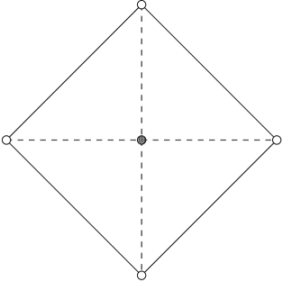
Figure 1: The soliton polytope of Landau-Ginzburg theory with the superpotential $W^{[2,2]}(\Phi^{1},\Phi^{2})={(\Phi^{1})^{5}\over 5}-(\Phi^{1})^{3}\Phi^{2}+\Phi^{1}(\Phi^{2})^{2}-\mu\Phi^{1}$. Each circle represents the critical point on the $W$-plane and the line connecting them is the soliton in the Landau-Ginzburg theory.

We can find two types of solitons; one is the edges of the quadrangle described by solid lines and the other is the diagonal line of the quadrangle described by broken lines in Figure 1. The number of solitons is four for edges and two for diagonal lines and the ratio of the lengths is $\sin(\pi/4)$. These are exactly the ones which correspond to the boundary states in the Kazama-Suzuki model listed above.

Now we will give an interpretation of label $m$ that will specify the direction of the soliton in the soliton polytopes. Let us consider a level-rank duality:

$$\frac{\widehat{SU}(3)_{1}\times\widehat{SO}(4)_{1}}{\widehat{SU}(2)_{2}\times\widehat{U}(1)_{24}}\cong\frac{\widehat{SU}(2)_{2}\times\widehat{SO}(2)_{1}}{\widehat{U}(1)_{8}}~{}.$$ (4.5)

The right hand side of (4.5) is nothing but the ${\cal N}=2$ minimal model at level 2. The known fact is that boundary states in this model is related to the solitons in the Landau-Ginzburg theory [21, 22, 23, 24]. The boundary states in the ${\cal N}=2$ minimal model at level $2$ are classified by the label $(\ell,m^{\prime},s)$ of the primary fields, where

$$0\leq\ell\leq 2~{},\quad m^{\prime}\in{\bf Z}_{8}~{},\quad s\in{\bf Z}_{4}~{},\quad\ell+m^{\prime}+s=0~{}~{}{\rm mod}~{}2~{},$$ (4.6)

$$(\ell,m^{\prime},s)\sim(2-k,m^{\prime}+4,s+2)~{}.$$ (4.7)

After the field identification, independent boundary states in ${\cal N}=2$ minimal model are given as follows:

$${|0,m^{\prime},s\rangle}~{}, \quad m^{\prime}\in 2{\bf Z}~{}{\rm mod}~{}8~{},$$

$${|1,m^{\prime}+1,s\rangle}~{}, \quad m^{\prime}\in 2{\bf Z}~{}{\rm mod}~{}4~{}.$$ (4.8)

For simplicity, we set $s=0$, since it only represents the orientation of the soliton (or brane). Then the state ${|0,m^{\prime},0\rangle}$ corresponds to the edge line of the quadrangle and it generates a phase factor $e^{i\pi m^{\prime}\over 4}$ which gives the direction of the soliton. Similarly the state ${|1,m^{\prime}+1,0\rangle}$ corresponds to the diagonal line of quadrangle and its phase factor is $e^{i\pi(m^{\prime}+1)\over 4}$ .

Now let us observe the correspondence between the boundary states in ${\cal N}=2$ minimal model and those in Kazama-Suzuki model. This can be easily checked by comparing the conformal dimension and the $U(1)$ charge of each primary state. The result is

$${|0,m^{\prime},0\rangle} \Longleftrightarrow {|(0,0),0,3m^{\prime},m^{\prime}\rangle}$$ (4.9)

$${|1,m^{\prime}+1,0\rangle} \Longleftrightarrow {|(0,0),1,3m^{\prime}+3,m^{\prime}+1\rangle}$$ (4.10)

where $m^{\prime}$ takes values in $0,2,4,6$ ($3m^{\prime}={\tilde{m}}=6{\bf Z}$ mod 24). Thus we were able to succeed to identify the boundary states of the Kazama-Suzuki model and the solitons in Landau-Ginzburg theory.

On the other hand, there are some solitons that could not be identified with the boundary states. For example, we cannot find a boundary state corresponding to a soliton that connects the origin with any other critical point. Moreover when we consider other models at even level $k$, we always find some critical points at the origin. However we cannot identify the boundary states with such solitons which connects the origin with any other critical point. On the contrary, as far as we checked, the boundary states in Kazama-Suzuki model can always be identified with the solitons in Landau-Ginzburg theory even though we change the level or rank of the model (2.2). This may reflect the fact that we only consider the boundary states which satisfy the untwisted boundary condition. Therefore other solitons may be identified with the boundary states satisfying the twisted boundary conditions [38] which do not break the A-type boundary condition [31, 32].

4.2 Example 2

Next we consider the following coset model at level 2:

$$\frac{\widehat{SU}(3)_{2}\times\widehat{SO}(4)_{1}}{\widehat{SU}(2)_{3}\times\widehat{U}(1)_{30}}~{}.$$ (4.11)

After using the field identification rule, inequivalent states which label the primary fields in the coset model (4.11) are given as follows:

$$((0,0),0,m,s)~{},\quad((0,0),1,m+3,s)~{},$$ (4.12)

$$((1,1),0,m,s)~{},\quad((1,1),1,m+3,s)~{},$$ (4.13)

where we should note that $m=6{\bf Z}$ mod 30 from the selection rule. Then we can calculate the mass of each boundary state.

Boundary state	Mass
${|({\tilde{\ell}}_{1},{\tilde{\ell}}_{2}),{\tilde{\lambda}},{\tilde{m}},{\tilde{s}}\rangle}$	$M(({\tilde{\ell}}_{1},{\tilde{\ell}}_{2}),{\tilde{\lambda}},{\tilde{m}},{\tilde{s}})$
${|(0,0),0,{\tilde{m}},{\tilde{s}}\rangle}$	$\left(\sin{\pi\over 5}\right)^{3}\sin{2\pi\over 5}\;$
${|(0,0),1,{\tilde{m}}+3,{\tilde{s}}\rangle}$	$\left(\sin{\pi\over 5}\right)^{2}\left(\sin{2\pi\over 5}\right)^{2}$
${|(1,1),0,{\tilde{m}},{\tilde{s}}\rangle}$	$\left(\sin{\pi\over 5}\right)^{2}\left(\sin{2\pi\over 5}\right)^{2}$
${|(1,1),1,{\tilde{m}}+3,{\tilde{s}}\rangle}$	$\sin{\pi\over 5}\,\left(\sin{2\pi\over 5}\right)^{3}$

Furthermore, by analogy with the previous example it is natural to propose that each boundary state in Kazama-Suzuki model should give a phase factor $e^{i\pi m^{\prime}\over 5}$ or $e^{i\pi(m^{\prime}+1)\over 5}$, where $3m^{\prime}={\tilde{m}}=6{\bf Z}$ mod 30, when we compare these boundary states with the solitons in the Landau-Ginzburg theory.

We then consider the solitons of Landau-Ginzburg theory which should be identified with the boundary states in the model (4.11). Corresponding Landau-Ginzburg superpotential is

$$W^{[2,3]}(\Phi^{1},\Phi^{2})={(\Phi^{1})^{6}\over 6}-(\Phi^{1})^{4}\Phi^{2}+{2\over 3}(\Phi^{1})^{2}(\Phi^{2})^{2}-(\Phi^{2})^{3}-\mu\Phi^{1}~{}.$$ (4.14)

By using this superpotential, we can calculate the critical points and draw a picture of soliton polytope of the theory (see Figure 2).

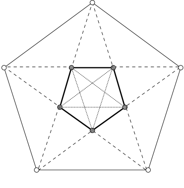
Figure 2: The soliton polytope of Landau-Ginzburg theory with the superpotential $W^{[2,3]}(\Phi^{1},\Phi^{2})={(\Phi^{1})^{6}\over 6}-(\Phi^{1})^{4}\Phi^{2}+{2\over 3}(\Phi^{1})^{2}(\Phi^{2})^{2}-(\Phi^{2})^{3}-\mu\Phi^{1}$.

There are ten critical points on the W-plane. Among them, five points form a small pentagon (described by filled circles in Figure 2) and the other five points form a big pentagon (described by white circles). We can find four types of solitons which can be identified as the boundary states of Kazama-Suzuki model. The first solitons are represented by the thick solid lines which connect two neighboring filled circles and they form a small pentagon. The second solitons are represented by dotted lines and they form a small star. The third solitons are represented by broken lines which connect a white circle to a filled circle. Final solitons are represented by solid lines which connect two neighboring white circles and they form a big pentagon. The interesting observation about these four types of solitons is that the ratio of the lengths is exactly equal to the mass ratio of the boundary states. Precisely speaking, the thick solid lines correspond to the boundary states ${|(0,0),0,{\tilde{m}},{\tilde{s}}\rangle}$, the dotted lines correspond to the boundary states ${|(0,0),1,{\tilde{m}}+3,{\tilde{s}}\rangle}$, the broken lines correspond to the boundary states ${|(1,1),0,{\tilde{m}},{\tilde{s}}\rangle}$ and finally the solid lines correspond to the boundary states ${|(1,1),1,{\tilde{m}}+3,{\tilde{s}}\rangle}$. One might be afraid that it is impossible to distinct between ${|(0,0),1,{\tilde{m}}+3,{\tilde{s}}\rangle}$ and ${|(1,1),0,{\tilde{m}},{\tilde{s}}\rangle}$ because they give the same mass. However as we mentioned before, these boundary states should give a phase factor $e^{i\pi(m^{\prime}+1)\over 5}$ and $e^{i\pi m^{\prime}\over 5}$, respectively and thus the relative angle differs by ${\pi\over 5}$. By taking account of the phase factors, we can identify all the boundary states in the model (4.11) with the solitons drawn in the soliton polytope of the Landau-Ginzburg theory.

On the other hand, there is a problem. There are ten broken lines in the soliton polytope as opposed to the fact that there are only five boundary states ${|(1,1),0,{\tilde{m}},{\tilde{s}}\rangle}$ (${\tilde{m}}=0,6,12,18,24$). However the disagreement could not be a serious problem since among the ten solitons, five of them have independent directions. Therefore the boundary states may correspond to such independent solitons.

Finally, we should comment on the $SU(3)/SU(2)\times U(1)$ models at an arbitrary level $k$. On the Landau-Ginzburg side, the critical points essentially form some regular $(k+3)$-gons on the $W$-plane and all of the $(k+3)$-gons have the equal center with the different sizes [19]. In particular, when the level $k$ is even, the solitons which have the smallest mass always correspond to the edges of the smallest $(k+3)$-gon. (When the level $k$ is odd, we always find the degenerate critical points at the origin.) On the other hand, the boundary states in the Kazama-Suzuki model are labeled by ${|({\tilde{\ell}}_{1},{\tilde{\ell}}_{2}),{\tilde{\lambda}},{\tilde{m}},{\tilde{s}}\rangle}$. Now let us consider the state ${|(0,0),0,{\tilde{m}},0\rangle}$ which have the smallest mass among all the boundary states. Then the label ${\tilde{m}}$ takes values in ${\tilde{m}}=6{\bf Z}~{}~{}{\rm mod}~{}~{}6(k+3)$ and it should give a phase factor $e^{\frac{2\pi i{\tilde{m}}}{6(k+3)}}$. Thus the states ${|(0,0),0,{\tilde{m}},0\rangle}$ can naturally be identified with the solitons represented by the edges of the smallest $(k+3)$-gon on the $W$-plane. Moreover, we can easily observe that the states ${|(0,0),{\tilde{\lambda}},{\tilde{m}}+3{\tilde{\lambda}},0\rangle}$ correspond to the solitons connecting the two arbitrary vertices of the smallest $(k+3)$-gon. Furthermore, as far as we checked, we can always find the solitons in the Landau-Ginzburg theory which correspond to the boundary states ${|({\tilde{\ell}}_{1},{\tilde{\ell}}_{2}),{\tilde{\lambda}},{\tilde{m}},{\tilde{s}}\rangle}$.

4.3 Geometrical interpretation of boundary states

Finally, we would like to discuss a geometrical interpretation of the boundary states in (perturbed) Kazama-Suzuki model. We will follow the work [5, 42] in this subsection and propose that the boundary states can be identified with the D4-branes wrapped on supersymmetric cycles.

For our starting point, we consider type IIA string theory on ${\bf R}^{1,1}\times Y$, where $Y$ is a compact Calabi-Yau four-fold. The vacuum structure of IIA string compactification is then obtained by choosing $Y$ and a flux for the 4-form field strength $G$ on $Y$. This flux $G$ originates from the field strength $G=dC$ of three-form potential $C$ in M-theory on ${\bf R}^{1,2}\times Y$ and the string theory is derived by circle compactification. In type IIA string theory, this flux is understood as the RR 4-form field. The difference between $\xi\equiv\left[G\over 2\pi\right]$ and $\xi^{\prime}$ is classified topologically by $\xi-\xi^{\prime}\in H^{4}(Y;{\bf Z})$. By Poincaré duality, $H_{4}(Y;{\bf Z})=H^{4}(Y;{\bf Z})$, there is a 4-cycle $S\subset X$ which represents an element of $H_{4}(Y;{\bf Z})$. The domain walls, or solitons, are then represented by kinks that interpolate between spatial regions in which $G$-fluxes are different. Indeed, D4-brane wrapped on a 4-cycle $S\in H_{4}(Y;{\bf Z})$ appears as a “particle” in the world ${\bf R}^{1,1}$ and can be regarded as a source of $G$-flux. If we across the particle, we arrive at a region in which $G$-flux is different. Thus this D4-brane looks macroscopically like a domain wall, or a soliton.

For practical reason, it is convenient to omit the part of $Y$ that is far from the singularity and to consider the non-compact Calabi-Yau four-fold $X$ that is developing a singularity. Let us consider Type IIA strings propagating on a singular Calabi-Yau four-fold whose singularity looks like the $A_{N-1}$ singular hypersurface

$$P_{N}(z_{1})+z_{2}^{2}+\ldots+z_{5}^{2}=0~{},$$ (4.15)

where $P_{N}(z_{1})$ is a polynomial of degree $N$ in $z_{1}$. Then for the holomorphic $4$-form $\Omega$ of the non-compact Calabi-Yau four-fold, the volume of a supersymmetric 4-cycle $C$ is given by [5]

$$V = \int_{C}\left|\Omega\right|$$ (4.16)

$$= \left|~{}\int_{I}P_{N}(z_{1})~{}dz_{1}~{}\right|~{},$$

where the one-dimensional line segment $I$ represent the image of the supersymmetric 4-cycle on the $z_{1}$ plane. If we define a function $W$ such that

$$dW(z_{1})=P_{N}(z_{1})~{}dz_{1}~{},$$ (4.17)

the volume of the cycle $C$ becomes

$$V=\left|~{}\int_{I_{ab}}dW~{}\right|=\left|W(\phi_{a})-W(\phi_{b})\right|~{},$$ (4.18)

where $z_{1}=\phi_{a}$ and $z_{1}=\phi_{b}$ are the end points of segment $I_{ab}$. Moreover the endpoints of the segment in the $z_{1}$ plane correspond to the critical points in W, namely $dW=0$ (or $P_{N}(z_{1})=0$). This condition is equivalent to find critical points in ${\cal N}=2$ Landau-Ginzburg theory with the superpotential $W$. Therefore we can identify the D4-branes wrapping on the supersymmetric cycles with the solitons in the Landau-Ginzburg theory interpolating between two critical points. Furthermore from the soliton/boundary state correspondence, it seems to be natural to identify the boundary state with the wrapped 4-branes.

When the polynomial $P_{N}(z_{1})$ represents the deformation of $A_{N-1}$ singularity;

$$P_{N}(z_{1})=(z_{1})^{N}-\mu\quad{\rm or}\quad W(z_{1})={(z_{1})^{N+1}\over N+1}-\mu z_{1}~{},$$ (4.19)

the D-branes wrapped on the supersymmetric 4-cycles of the singular Calabi-Yau four-fold are related with the boundary states in ${\cal N}=2$ minimal models [23]. The system they considered is closely related to the one considered in [5]. They considered the holographic dual description of singular Calabi-Yau compactification of type II string theory in the decoupling limit by making use of ${\cal N}=2$ minimal models and the ${\cal N}=2$ Liouville theory [6, 8]. The soliton structure corresponding to the wrapped D4-branes are essentially captured from the boundary states in ${\cal N}=2$ minimal model. They evaluated the period of the wrapped branes from the boundary states and derived the exact agreement with the geometrical calculation including the scaling behavior.

Now let us consider the Kazama-Suzuki models. As we mentioned before, the vacuum structure of the theory is determined not only by choosing $X$ but also by choosing a flux $G$ on $X$. To specify the theory on the non-compact Calabi-Yau manifold $X$, we have to fix the flux of $C$-field at the boundary $\partial X$, i.e. the region near infinity in $X$. From the quantization condition on the flux [5], the theory is determined by the constant flux, $\Phi$, measured at infinity;

$$\Phi=n+{1\over 2}\xi^{2}~{},$$ (4.20)

where $n$ is the number of “string”. However $n\neq 0$ state has massless excitations coming from the strings, then a model with a mass gap must have $n=0$. Therefore to get a theory that flows into the massive vacua only we need to determine minimal $\Phi$.

As was discussed in [5], when $X$ is described by the $A_{N-1}$ singular hypersurface (4.15), then the homology $H_{4}(X;{\bf Z})$ is naturally identified with the root lattice $\Gamma$ of $SU(N)$ and the intersection form is the Cartan matrix of the group. While the full set of non-trivial $G$-flux $\xi$ are classified by $H^{4}(X;{\bf Z})$ which can be identified with the weight lattice $\Gamma^{*}$ of $SU(N)$. Moreover the possible values of $\xi$ modulo the changes due to crossing the domain walls are classified by $\Gamma^{*}/\Gamma$, that is isomorphic to the center ${\bf Z}_{N}$ of $SU(N)$ [5]. The distinct elements of $\Gamma^{*}/\Gamma$ are defined by the congruence class (see for example, Chapter 13 of [43]). When the center is equal to $m$ ($m=0,1,\ldots,N-1$), $\xi$ must be the weight of $m$-fold anti-symmetric tensor product of fundamental representations of $SU(N)$ to minimize ${1\over 2}\xi^{2}$ in (4.20). If we denote the representation by $R_{m}$, then the number of choice of $\xi$ is then the dimension of $R_{m}$, i.e. ${\rm dim}(R_{m})=\frac{N!}{m!(N-m)!}$.

Now let us consider a few examples. At first, when $m=1$, then the dimension or the number of vacua becomes ${\rm dim}(R_{1})=N$, which is exactly the number of vacua of Landau-Ginzburg theory with the superpotential (4.19). Secondly, when $m=2$, then the dimension becomes ${\rm dim}(R_{2})={1\over 2}N(N-1)$. In particular, when $N=k+3=4,5$, the number of vacua is $6,10$, which are those of vacua in Landau-Ginzburg theory discussed in Example 1 and 2. Therefore we propose that the solitons which represent D4-branes wrapped on the supersymmetric 4-cycles can naturally be identified with the boundary states in Kazama-Suzuki model. In addition, the boundary states we considered satisfy the A-type boundary condition [31, 32] and they essentially correspond to the D-branes wrapping on the middle dimensional cycles, i.e. supersymmetric 4-cycles. This fact also supports our interpretation.

However, the crucial difficulty is that the Landau-Ginzburg theory describes the space-time CFT, on the other hand our Kazama-Suzuki model should describe the world-sheet CFT to give a correct meaning of boundary state. This difference might be related with the shift of level by one when we compared the solitons with the boundary states. Instead of dealing such a space-time CFT directly, the holographic dual description of superstring theory on a non-compact Calabi-Yau four-fold is proposed in [6, 8] by the ${\cal N}=2$ minimal model and the ${\cal N}=2$ Liouville theory. Then the deformation parameter $\mu$ of the Landau-Ginzburg theory (4.19) is identified with the parameter of perturbation by the cosmological constant operator in the ${\cal N}=2$ Liouville theory. Likewise, the Kazama-Suzuki model may appear in the holographic dual description of such a Calabi-Yau compactification with the RR-flux. We do not know whether this dual description is valid for any value of the RR-flux. However the soliton structure sufficiently characterize the theory, and hence the strong relation with the boundary states in Kazama-Suzuki model would give the natural interpretation that the boundary states describe the BPS D4-branes.

We do not know, so far, any non-compact Calabi-Yau compactification by use of Kazama-Suzuki models. It would be interesting to construct the consistent modular invariant theory combined in the ${\cal N}=2$ Liouville theory or its generalization.

5 Summary and discussions

We studied the correspondence between the boundary states in Kazama-Suzuki models and the solitons in Landau-Ginzburg theories. We have found the successful correspondence by comparing the mass of boundary state with the one of soliton including the direction on the $W$-plane. We further discussed a geometrical interpretation of the boundary states in Kazama-Suzuki models and proposed that the boundary states are naturally identified with the D4-branes wrapping on a supersymmetric cycles in a non-compact Calabi-Yau four-fold with an appropriate RR-flux.

On the other hand, there is an open problem that the number of the solitons in the Landau-Ginzburg theory is much larger than that of the boundary states in Kazama-Suzuki models. This problem occur even if we change the level or rank of the models. However we only consider the boundary states which satisfy the untwisted boundary condition. Hence it is interesting to consider the boundary states which satisfy the twisted boundary conditions [38, 32].

Moreover it is important to clarify the relation between the space-time CFT which is realized as the IR fixed point of two dimensional field theory obtained from a singular Calabi-Yau four-fold compactification and the world-sheet CFT described by the Kazama-Suzuki model. In this paper, we take a position that the the solitons in the space-time Landau-Ginzburg theory are related to the boundary states in the world-sheet Kazama-Suzuki model in a sense of holography [6, 23]. To completely understand this relation, it is important to construct the modular invariant partition function which satisfy the condition of critical dimension and evaluate the periods of the supersymmetric cycles. This construction is not well understood so far and may be achieved by combining with the Liouville theory or its generalization [44].

Finally in this paper, we have only discussed the Grassmannian models, in particular we explicitly checked the correspondence between the boundary states and the solitons in a few simple models. It is therefore important to check this correspondence for other levels or ranks to understand the general correspondence. It would be also interesting to check this correspondence for other SLOHSS models [12, 14]. Moreover, as in the ${\cal N}=2$ minimal model cases [20, 34], it is valuable to discuss the geometrical meaning of intersection forms in Kazama-Suzuki models [25].

Appendix A S-matrices in Kazama-Suzuki model

In the appendix, we summarize S-matrices appeared in the Kazama-Suzuki model.

$SU(n+1)$ WZW model

Let us denote the highest weight of $SU(n+1)$ at level $k$ as $\Lambda$. Then modular transformation S-matrix for $SU(n+1)$ WZW model at level $k$ can formally be written in the following way:

$$S_{\Lambda,{\tilde{\Lambda}}}^{SU(n+1)}=\frac{i^{{1\over 2}n(n+1)}}{\sqrt{n+1}(k+n+1)^{n/2}}\sum_{w\in W}\epsilon(w)e^{-2\pi iw(\Lambda+\rho)({\tilde{\Lambda}}+\rho)/(k+n+1)}~{},$$ (A.1)

where $W$ denotes the Weyl group of $SU(n+1)$ and $\rho$ is the Weyl vector.

$SU(3)$ WZW model

We denote the highest weights of $SU(3)$ at level $k$ as $\lambda$ and it is labeled by

$${\cal P}_{+}^{k}=\{\Lambda=\ell_{1}\omega_{1}+\ell_{2}\omega_{2}|\ell_{1},\ell_{2}\in{\bf Z},\;0\leq\ell_{1},\ell_{2},\;\ell_{1}+\ell_{2}\leq k\}~{},$$ (A.2)

where $\omega_{1}$ and $\omega_{2}$ are fundamental weights of $SU(3)$. Then a explicit form of the modular S-matrix for $SU(3)$ WZW model at level $k$ can be written in the following way:

$$(S^{SU(3)})_{\lambda,\lambda^{\prime}}\!\! = \frac{-i}{\sqrt{3}(k+1)}\left\{e^{{-2\pi i\over 3(k+3)}[2(\ell_{1}+1)(\ell_{1}^{\prime}+1)+(\ell_{1}+1)(\ell_{2}^{\prime}+1)+(\ell_{2}+1)(\ell_{1}^{\prime}+1)+2(\ell_{2}+1)(\ell_{2}^{\prime}+1)]}\right.$$ (A.3)

$$\quad\quad\quad\quad\;\;\,+e^{{-2\pi i\over 3(k+3)}[-(\ell_{1}+1)(\ell_{1}^{\prime}+1)-2(\ell_{1}+1)(\ell_{2}^{\prime}+1)+(\ell_{2}+1)(\ell_{1}^{\prime}+1)-(\ell_{2}+1)(\ell_{2}^{\prime}+1)]}$$

$$\quad\quad\quad\quad\;\;\,+e^{{-2\pi i\over 3(k+3)}[-(\ell_{1}+1)(\ell_{1}^{\prime}+1)+(\ell_{1}+1)(\ell_{2}^{\prime}+1)-2(\ell_{2}+1)(\ell_{1}^{\prime}+1)-(\ell_{2}+1)(\ell_{2}^{\prime}+1)]}$$

$$\quad\quad\quad\quad\;\;\,-e^{{-2\pi i\over 3(k+3)}[-(\ell_{1}+1)(\ell_{1}^{\prime}+1)-2(\ell_{1}+1)(\ell_{2}^{\prime}+1)-2(\ell_{2}+1)(\ell_{1}^{\prime}+1)-(\ell_{2}+1)(\ell_{2}^{\prime}+1)]}$$

$$\quad\quad\quad\quad\;\;\,-e^{{-2\pi i\over 3(k+3)}[2(\ell_{1}+1)(\ell_{1}^{\prime}+1)+(\ell_{1}+1)(\ell_{2}^{\prime}+1)+(\ell_{2}+1)(\ell_{1}^{\prime}+1)-(\ell_{2}+1)(\ell_{2}^{\prime}+1)]}$$

$$\quad\quad\quad\quad\;\;\,\left.-e^{{-2\pi i\over 3(k+3)}[-(\ell_{1}+1)(\ell_{1}^{\prime}+1)+(\ell_{1}+1)(\ell_{2}^{\prime}+1)+(\ell_{2}+1)(\ell_{1}^{\prime}+1)+2(\ell_{2}+1)(\ell_{2}^{\prime}+1)]}\right\}$$

$\widehat{U}(1)_{L}$ model

The modular S-matrix for $U(1)$ model at level $L$ is given by

$$S_{m,{\tilde{m}}}^{U(1)}={1\over\sqrt{L}}e^{-{2\pi im{\tilde{m}}\over L}}$$ (A.4)

where $m,{\tilde{m}}\in{\bf Z}_{L}$.

$\widehat{SO}(2n)_{1}$ model

In general, the character of $\widehat{SO}(2n)_{1}$ is given by

$$\chi_{0}^{SO(2n)}={1\over 2}\left[\left(\theta_{3}\over\eta\right)^{n}+\left(\theta_{4}\over\eta\right)^{n}\right]~{}, \chi_{2}^{SO(2n)}={1\over 2}\left[\left(\theta_{3}\over\eta\right)^{n}-\left(\theta_{4}\over\eta\right)^{n}\right]~{},$$

$$\chi_{1}^{SO(2n)}={1\over 2}\left[\left(\theta_{2}\over\eta\right)^{n}+\left(-i\theta_{1}\over\eta\right)^{n}\right]~{}, \chi_{-1}^{SO(2n)}={1\over 2}\left[\left(\theta_{2}\over\eta\right)^{n}-\left(-i\theta_{1}\over\eta\right)^{n}\right]~{},$$

or

$$\chi_{0}^{SO(2n)}+\chi_{2}^{SO(2n)}=\left(\theta_{3}\over\eta\right)^{n}~{}, \chi_{0}^{SO(2n)}-\chi_{2}^{SO(2n)}=\left(\theta_{4}\over\eta\right)^{n}~{},$$

$$\chi_{1}^{SO(2n)}+\chi_{-1}^{SO(2n)}=\left(\theta_{2}\over\eta\right)^{n}~{}, \chi_{1}^{SO(2n)}-\chi_{-1}^{SO(2n)}=\left(-i\theta_{1}\over\eta\right)^{n}~{}.$$

The modular S-matrix of character $\chi_{s}^{SO(2n)}(\tau)$ ($s=0,2,1,-1$) is

$$S_{s,{\tilde{s}}}^{SO(2n)}={1\over 2}\left(\begin{array}[]{cccc}1&1&1&1\\ 1&1&-1&-1\\ 1&-1&i^{-n}&-i^{-n}\\ 1&-1&-i^{-n}&i^{-n}\end{array}\right)~{}.$$ (A.5)

For $n={\rm odd}$ case, the above matrix can be simply expressed as

$$S_{s,{\tilde{s}}}^{SO(2n)}={1\over 2}e^{-{n\pi i\over 2}s{\tilde{s}}}~{}.$$ (A.6)

References

- [1] A. Strominger, “Massless black holes and conifolds in string theory,” Nucl. Phys. B 451 (1995) 96, hep-th/9504090.
- [2] B. R. Greene, D. R. Morrison and A. Strominger, “Black hole condensation and the unification of string vacua,” Nucl. Phys. B 451 (1995) 109, hep-th/9504145.
- [3] H. Ooguri and C. Vafa, “Two-dimensional black hole and singularities of CY manifolds,” Nucl. Phys. B463 (1996) 55, hep-th/9511164.
- [4] O. Aharony, M. Berkooz, D. Kutasov and N. Seiberg, “Linear dilatons, NS5-branes and holography,” JHEP 9810 (1998) 004, hep-th/9808149.
- [5] S. Gukov, C. Vafa and E. Witten, “CFT’s from Calabi-Yau four-folds,” Nucl. Phys. B 584 (2000) 69, [Erratum-ibid. B 608 (2000) 477], hep-th/9906070.
- [6] A. Giveon, D. Kutasov and O. Pelc, “Holography for non-critical superstrings,” JHEP 9910 (1999) 035, hep-th/9907178.
- [7] A. Giveon, D. Kutasov, “Little string theory in a double scaling limit,” JHEP 9910 (1999) 034, hep-th/9909110; A. Giveon, D. Kutasov, “Comments on double scaled little string theory,” JHEP 0001 (2000) 023, hep-th/9911039.
- [8] T. Eguchi and Y. Sugawara, “Modular invariance in superstring on Calabi-Yau n-fold with A-D-E singularity,” Nucl. Phys. B 577 (2000) 3, hep-th/0002100.
- [9] S. Mizoguchi, “Modular invariant critical superstrings on four-dimensional Minkowski space x two-dimensional black hole,” JHEP 0004 (2000) 014, hep-th/0003053.
- [10] S. Yamaguchi, “Gepner-like description of a string theory on a non-compact singular Calabi-Yau manifold,” Nucl. Phys. B 594 (2001) 190, hep-th/0007069.
- [11] M. Naka and M. Nozaki, “Singular Calabi-Yau manifolds and ADE classification of CFTs,” Nucl. Phys. B 599 (2001) 334, hep-th/0010002.
- [12] Y. Kazama and H. Suzuki, “New N=2 Superconformal Field Theories And Superstring Compactification,” Nucl. Phys. B 321 (1989) 232; Y. Kazama and H. Suzuki, “Characterization Of N=2 Superconformal Models Generated By Coset Space Method,” Phys. Lett. B 216 (1989) 112.
- [13] W. Lerche, C. Vafa and N. P. Warner, “Chiral Rings In N=2 Superconformal Theories,” Nucl. Phys. B 324 (1989) 427.
- [14] W. Lerche and N. P. Warner, “Polytopes and solitons in integrable, N=2 supersymmetric Landau-Ginzburg theories,” Nucl. Phys. B 358 (1991) 571.
- [15] D. Gepner, “Fusion rings and geometry,” Commun. Math. Phys. 141 (1991) 381.
- [16] K. A. Intriligator, “Fusion residues,” Mod. Phys. Lett. A 6 (1991) 3543, hep-th/9108005.
- [17] S. Cecotti and C. Vafa, “On classification of N=2 supersymmetric theories,” Commun. Math. Phys. 158 (1993) 569, hep-th/9211097.
- [18] E. Witten, “The Verlinde algebra and the cohomology of the Grassmannian,” hep-th/9312104.
- [19] P. Di Francesco, F. Lesage and J. B. Zuber, “Graph rings and integrable perturbations of N=2 superconformal theories,” Nucl. Phys. B 408 (1993) 600, hep-th/9306018.
- [20] K. Hori, A. Iqbal and C. Vafa, “D-branes and mirror symmetry,” hep-th/0005247.
- [21] W. Lerche, “On a boundary CFT description of nonperturbative N = 2 Yang-Mills theory,” hep-th/0006100.
- [22] W. Lerche, C. A. Lutken and C. Schweigert, “D-branes on ALE spaces and the ADE classification of conformal field theories,” hep-th/0006247.
- [23] T. Eguchi and Y. Sugawara, “D-branes in singular Calabi-Yau n-fold and N = 2 Liouville theory,” Nucl. Phys. B 598 (2001) 467, hep-th/0011148.
- [24] K. Sugiyama and S. Yamaguchi, “D-branes on a noncompact singular Calabi-Yau manifold,” JHEP 0102 (2001) 015, hep-th/0011091; S. Yamaguchi, “Noncompact Gepner models with discrete spectra,” Phys. Lett. B 509 (2001) 346, hep-th/0102176.
- [25] W. Lerche and J. Walcher, “Boundary rings and N = 2 coset models,” hep-th/0011107.
- [26] J. L. Cardy, “Boundary Conditions, Fusion Rules And The Verlinde Formula,” Nucl. Phys. B 324 (1989) 581.
- [27] D. Gepner, “Scalar Field Theory And String Compactification,” Nucl. Phys. B 322 (1989) 65.
- [28] S. G. Naculich and H. J. Schnitzer, “Superconformal coset equivalence from level-rank duality,” Nucl. Phys. B 505 (1997) 727, hep-th/9705149.
- [29] A. N. Schellekens, “Field identification fixed points in N=2 coset theories,” Nucl. Phys. B 366 (1991) 27.
- [30] D. Gepner, “Field Identification In Coset Conformal Field Theories,” Phys. Lett. B 222 (1989) 207.
- [31] H. Ooguri, Y. Oz and Z. Yin, “D-branes on Calabi-Yau spaces and their mirrors,” Nucl. Phys. B477 (1996) 407, hep-th/9606112.
- [32] S. Stanciu, “D-branes in Kazama-Suzuki models,” Nucl. Phys. B 526 (1998) 295, hep-th/9708166.
- [33] N. Ishibashi, “The Boundary And Crosscap States In Conformal Field Theories,” Mod. Phys. Lett. A 4 (1989) 251.
- [34] J. Maldacena, G. W. Moore and N. Seiberg, “Geometrical interpretation of D-branes in gauged WZW models,” JHEP 0107 (2001) 046, hep-th/0105038.
- [35] K. Gawedzki, “Boundary WZW, G/H, G/G and CS theories,” hep-th/0108044.
- [36] S. Elitzur and G. Sarkissian, “D-branes on a gauged WZW model,” hep-th/0108142.
- [37] S. Fredenhagen and V. Schomerus, “D-branes in coset models,” hep-th/0111189.
- [38] H. Ishikawa, “Boundary states in coset conformal field theories,” hep-th/0111230.
- [39] E. J. Martinec, “Algebraic Geometry And Effective Lagrangians,” Phys. Lett. B 217 (1989) 431.
- [40] C. Vafa and N. P. Warner, “Catastrophes And The Classification Of Conformal Theories,” Phys. Lett. B 218 (1989) 51.
- [41] P. Fendley, S. D. Mathur, C. Vafa and N. P. Warner, “Integrable Deformations And Scattering Matrices For The N=2 Supersymmetric Discrete Series,” Phys. Lett. B 243 (1990) 257.
- [42] T. Eguchi, N. P. Warner and S. K. Yang, “ADE singularities and coset models,” Nucl. Phys. B 607 (2001) 3, hep-th/0105194.
- [43] P. Di Francesco, P. Mathieu and D. Senechal, “Conformal Field Theory,” New York, USA: Springer (1997).
- [44] M. Bershadsky, W. Lerche, D. Nemeschansky and N. P. Warner, “Extended N=2 superconformal structure of gravity and W gravity coupled to matter,” Nucl. Phys. B 401 (1993) 304, hep-th/9211040.