Searching for Quantum Solitons in a 3+1 Dimensional Chiral Yukawa Model

E. Farhi^a,, N. Graham^b, R.L. Jaffe^a, and H. Weigel^c,

ABSTRACT

We search for static solitons stabilized by heavy fermions in a 3+1 dimensional Yukawa model. We compute the renormalized energy functional, including the exact one-loop quantum corrections, and perform a variational search for configurations that minimize the energy for a fixed fermion number. We compute the quantum corrections using a phase shift parameterization, in which we renormalize by identifying orders of the Born series with corresponding Feynman diagrams. For higher-order terms in the Born series, we develop a simplified calculational method. When applicable, we use the derivative expansion to check our results. We observe marginally bound configurations at large Yukawa coupling, and discuss their interpretation as soliton solutions subject to general limitations of the model.

PACS: 05.45.Yv, 11.27.+d, 11.30.Rd, 11.10.Gh.

Keywords:  Solitons, Quantum Corrections, Vacuum Polarization Energy, Renormalization, Variational Methods.

1. Introduction and Motivation

Chiral gauge theories, such as the electroweak Standard Model, present a challenge to conventional notions of decoupling. By increasing its Yukawa coupling, one can make a fermion so heavy that it should be irrelevant to low-energy physics. On the other hand, it cannot simply disappear from the theory, since then anomalies would no longer cancel. It is known that decoupling a chiral fermion leaves behind a Wess-Zumino-Witten functional of the Higgs and gauge fields, which keeps the path integral gauge invariant [1]. However, to cancel Witten’s non-perturbative $SU(2)$ anomaly [2], an even number of chiral doublets must be present in the low-energy theory. After decoupling a fundamental fermion, the presence of a fermionic soliton in the low-energy theory would ensure that gauge invariance is maintained at the level of the states [1].

There is a natural mechanism for realizing this scenario. A twisted configuration of the Higgs field will cause one fermion level to become very tightly bound, or even to cross zero energy [3]. In the former case, the level can be filled at very little cost in energy, while in the latter case the background field itself carries fermion number. This energy must be added to the classical energy required to twist the Higgs field, and then compared to the mass of a fermion in an unperturbed background. However, one must also include the contribution of the shift in the zero-point energies of all the fermion modes, since it is of the same order in $\hbar$ as the energy of the filled level. If the total energy of a fermion number one twisted configuration is below the mass of a free fermion, then the configuration is stable.

In this paper, we explore this phenomenon in a simplified version of the electroweak sector of the Standard Model. We consider a Higgs doublet chirally coupled to a single heavy fermion doublet. We assume the fermions in the doublet have equal masses, and consider a hedgehog configuration for the Higgs field. We ignore the SU(2)_L-gauge fields. As we will argue in our conclusions, this may be an important omission, and work is currently underway to extend the calculation to include that case.

Previous work [4] showed that quantum-stabilized chiral solitons do exist in the one-dimensional analog of the model we are considering. Here, as in that work, we will consider only the quantum correction from the fermion loop, which we expect to be the most important effect. Neglecting bosonic loops is rigorously justified in the large $N$ limit, where $N$ is the number of independent fermion species, but here we couple to only a single doublet and take $N=1$.

Our methods allow us to evaluate the one-loop fermion contribution to the energy exactly, maintaining a fixed renormalization scheme while exploring different Higgs backgrounds. There have been earlier attempts to compute the one fermion loop energy for a three-dimensional chiral background within various approximation schemes. Examples include discretization methods [5, 6], which may not be rigorously valid in the continuum limit and require cutoffs, making the renormalization obscure. Other approaches use expansions that are valid for slowly [7] or rapidly [6, 8] varying background fields. Also truncations [9] in the potential generated by the background field, the heat kernel expansion [10], and subsets of field configurations with less severe ultraviolet divergences [11] have been studied. While these methods may be appropriate for specific applications and useful within certain regions in configuration or parameter space, they do not allow one to explore a full range of ansätze for the Higgs background or to make definitive statements about the existence of a soliton.

We include in this Introduction a brief review of our method for computing the contribution to the energy from vacuum polarization induced by the background field. For a fuller discussion of the method see Ref. [12, 13].

The vacuum polarization energy is given formally by a sum over bound states and an integral over continuum energies in the background given by $\Phi$,

$$\frac{1}{2}\sum_{j}\epsilon_{j}+\frac{1}{2}\int dk\frac{dn}{dk}\omega(k)$$ (1)

where $\{\epsilon_{j}\}$ are the bound state energies, $\omega(k)=\sqrt{k^{2}+m^{2}}$ is the energy of a scattering state, and ${dn}/{dk}$ is the change the continuum density of states due to the background field. ${dn}/{dk}$ can be calculated from the derivative of the phase shifts with respect to $k$ [14],

$$\frac{dn}{dk}=\frac{1}{2\pi i}\,{\rm tr}\ln S(k)=\frac{1}{\pi}\frac{d}{dk}\sum_{\ell}D(\ell)\delta(k,\ell)$$ (2)

where we have expanded the $S$ matrix in partial waves labeled by $\ell$, representing quantum numbers like angular momentum and parity. $\delta(k,\ell)$ gives the phase shift and $D(\ell)$ the degeneracy. Since we will consider cases where the spectrum is asymmetric in energy, we define $\delta(k,l)$ to be the sum of the phase shifts over both signs of the energy: $\delta(k,l)=\delta_{+}(k,l)+\delta_{-}(k,l)$, where $\pm$ specifies $\omega=\pm\sqrt{k^{2}+m^{2}}$.

Before we can do the $k$ integral, we must deal with potential divergences. We regulate the theory by dimensional regularization, that is, we analytically continue the entire theory to $n$ dimensions, where the integrals converge. For integer $n$, the expected divergences emerge from the high momentum behavior of the phase shift integral. At high momentum, the Born series becomes a good approximation to the phase shift, so by subtracting successive terms in the Born series from $\delta(k,l)$, we can remove terms from the $k$-integration that would diverge at physical values of $n$. The expansion in the Born series can then be unambiguously identified with the expansion of the effective energy in terms of Feynman diagrams with insertions of the background field [11, 12, 13]. In noninteger dimensions, the contributions of both the Born terms and the Feynman diagrams to the vacuum polarization energy are finite and unambiguous analytic functions of $n$. Therefore, when we subtract a term in the Born expansion and add back the equivalent Feynman diagram, we can be certain that we are not introducing finite ambiguities into the computation. The subtracted integration over the density of states is then finite and we can take the limit to integer $n$ without difficulty. Finally, we introduce the contributions from the counterterms, which have been computed using standard renormalization conditions in the perturbative sector of the model. As usual, the potentially divergent pieces of the Feynman diagram are canceled by the counterterm contributions. In all, the renormalized vacuum polarization energy is given by

$$E_{\rm vac} = \pm\left(\sum_{j}D(j)\epsilon_{j}+\int_{0}^{\infty}\frac{dk}{2\pi}\sqrt{k^{2}+m^{2}}\frac{d}{dk}\sum_{l}D(l)\left(\delta(k,l)-\sum_{N=1}^{N_{\rm max}}\delta^{(N)}(k,l)\right)\right)$$ (3)

$$\qquad{}+\sum_{N=1}^{N_{\rm max}}\Gamma^{(N)}(\Lambda)+\Gamma_{\rm ct}(\Lambda)$$

for bosons and fermions respectively, where the $N^{\rm th}$-order Born approximant to the phase shifts is denoted by $\delta^{(N)}(k,l)$. $N_{\rm max}$ is the number of Born subtractions required to render the $k$ integration finite. The compensating Feynman diagrams are denoted by $\Gamma^{(N)}(\Lambda)$, and $\Gamma_{\rm ct}(\Lambda)$ represents the contribution of the counterterms. Both are cutoff-dependent, but as usual, renormalization conditions will determine an unambiguous, finite result. We are left with two finite and numerically tractable objects, the momentum integral and the sum $\sum_{N=1}^{N_{\rm max}}\Gamma^{(N)}+\Gamma_{\rm ct}$. As a result, no explicit cutoff needs to be introduced in the numerical computation.

This paper is organized as follows. In Section 2 we briefly review the Higgs sector of the standard model and outline its connection to the Yukawa model. In Section 3 we discuss the renormalization of the fermion loop and describe our calculation of the associated contribution to the energy. Section 4 contains the numerical analysis. We summarize and provide an outlook on future studies in Section 5. Technical details are given in three Appendices. In Appendix A we explore the Dirac equation and its scattering solutions for a chiral background field. In Appendix B we describe and numerically verify a simplified treatment of contributions to the renormalized vacuum polarization energy that are higher order in the background field. In Appendix C we derive results in the derivative expansion, which we use to check our results in the case of slowly varying background fields.

2. The Model

The model we consider consists of the Higgs sector of the Standard Model coupled to a fermion doublet in $3+1$ dimensions. Our goal is to explore the possibility that within this model there is a non-trivial Higgs field configuration with nonzero fermion number whose energy is less than that of a state with the same quantum numbers built on top of the perturbative vacuum. The fermions get their masses through their Yukawa coupling to the Higgs. Our model differs in two essential ways from the Standard Model: we omit gauge fields and our fermions have equal masses. At the end of the paper we discuss the possible sensitivity of our results to the omission of gauge fields.

We write the Higgs sector of the Standard Model in terms of a $2\times 2$ matrix-valued Higgs field

$$\Phi=\pmatrix{\varphi_{0}&-\varphi_{+}^{*}\cr\varphi_{+}&\varphi_{0}^{*}}\,$$ (4)

where $(\varphi_{0},\varphi_{+})$ is the usual doublet. The Higgs Lagrangian is

$${\cal L}_{H}=\frac{1}{4}\,{\rm tr}\left[\partial_{\mu}\Phi^{\dagger}\partial^{\mu}\Phi\right]-V(\Phi)$$ (5)

where

$$V(\varphi)=\frac{\lambda}{16}\left({\rm tr}\left[\Phi^{\dagger}\Phi\right]-2v^{2}\right)^{2}\ .$$ (6)

We take the vacuum expectation value to be

$$\langle\Phi\rangle=v\pmatrix{1&0\cr 0&1}$$ (7)

and note that the Higgs particle has mass $m_{H}=\sqrt{\lambda}v$.

The coupling to the fermion doublet $q=(t,b)$ is given by

$${\cal L}_{\rm HF}=g\bar{q}_{L}\Phi q_{R}+g\bar{q}_{R}\Phi^{\dagger}q_{L}$$ (8)

which results in mass $m=gv$ for both $t$ and $b$. It is also convenient to rewrite $\Phi$ in terms of four real (dimensionless) fields $s$ and $\vec{p}$ as

$$\Phi=v\left(s+i\vec{\tau}\cdot\vec{p}\right)$$ (9)

which gives

$${\cal L}_{\rm HF}=m\bar{q}\left(s+i\gamma_{5}\vec{\tau}\cdot\vec{p}\right)q\ .$$ (10)

With these definitions, the classical energy is

$$E_{\rm cl}[\Phi]=\frac{v^{2}}{2}\int d^{3}r\left(\partial_{i}s\partial_{i}s+\partial_{i}\vec{p}\cdot\partial_{i}\vec{p}+\frac{\lambda v^{2}}{4}(s^{2}+\vec{p}\,^{2}-1)^{2}\right)\ .$$ (11)

3. The Fermion Loop

In this section we discuss the contribution of the fermion vacuum to the total energy. This contribution arises because the fermionic vacuum is polarized by the Higgs background. In order to compute this contribution we first have to outline the renormalization process in the perturbative sector of the model. The divergences of our model can be canceled by counterterms of the form

$${\cal L}_{\rm ct}=a\,{\rm tr}\,\left(\partial_{\mu}\Phi\partial^{\mu}\Phi^{\dagger}\right)-b\,{\rm tr}\,\left(\Phi\Phi^{\dagger}-v^{2}\right)-c\,{\rm tr}\,\left(\Phi\Phi^{\dagger}-v^{2}\right)^{2}$$ (12)

where $a$, $b$, and $c$ are cutoff-dependent constants. The Yukawa coupling $g$, and consequently the fermion mass $m$, are not renormalized at this order.

In terms of the shifted Higgs field $h\equiv s-v$, our renormalization conditions are that the vacuum expectation value of $h$ vanishes, and that the fermion loop changes neither the position $m_{H}$ nor the residue of the pole in the two-point function for $h$. In order to fix the counterterms, it is therefore sufficient to expand

$${\cal S}_{\rm eff}[h]=-i\,{\rm Tr}\,\ln\,\left\{i\partial\hskip-5.50003pt/-g(v+h)\right\}$$ (13)

up to quadratic order in $h$ and combine the result with $\int d^{4}x{\cal L}_{\rm ct}$. In dimensional regularization we obtain

$$a = -\frac{g^{2}}{(4\pi)^{2}}\left\{\frac{1}{\epsilon}-\gamma-\frac{2}{3}+\ln\,\left(\frac{4\pi\mu^{2}}{m^{2}}\right)-6\int_{0}^{1}dxx(1-x)\,\ln\,\left[1-x(1-x)\frac{m_{H}^{2}}{m^{2}}\right]\right\}$$

$$b = -\frac{g^{2}m^{2}}{(4\pi)^{2}}\left\{\frac{1}{\epsilon}-\gamma+1+\ln\,\left(\frac{4\pi\mu^{2}}{m^{2}}\right)\right\}$$

$$c = -\frac{g^{4}}{(4\pi)^{2}}\left\{\frac{1}{\epsilon}-\gamma+\ln\,\left(\frac{4\pi\mu^{2}}{m^{2}}\right)-\frac{m_{H}^{2}}{4m^{2}}-\frac{3}{2}\int_{0}^{1}dx\,\ln\,\left[1-x(1-x)\frac{m_{H}^{2}}{m^{2}}\right]\right\}$$ (14)

where $d=4-2\epsilon$, $\mu$ is the scale required to keep $g$ dimensionless.

Having set up the model in the perturbative sector, we now turn to non-trivial field configurations. We restrict our attention to the spherical ansatz for the Higgs field,

$$\Phi(\vec{x})=v\left[s(r)+i\vec{\tau}\cdot\hat{x}\,p(r)\right]$$ (15)

with $r=\sqrt{\vec{x}\,^{2}}$. With the standard form of the Dirac matrices, the corresponding Dirac operator becomes

$$h_{D}=\pmatrix{ms(r)&-i\vec{\sigma}\cdot\vec{\nabla}+mi\vec{\tau}\cdot\hat{x}\,p(r)\cr-i\vec{\sigma}\cdot\vec{\nabla}-mi\vec{\tau}\cdot\hat{x}\,p(r)&-ms(r)}$$ (16)

and the fermion field obeys the time-independent Dirac equation,

$$h_{D}\Psi=\omega\Psi\ .$$ (17)

Note that the energy eigenvalue $\omega$ can assume both positive and negative values. In general the spectrum of $h_{D}$ contains discrete (bound) and continuum (scattering) states.

First we obtain the bound states $\epsilon_{j}$, the solutions to eq. (17) with $|\omega|<m$. The numerical method is sketched in Appendix A. We can use Levinson’s theorem to compute the number of bound states in each channel from the phase shifts. The phase shifts are computed from the $S$-matrix, which in turn is extracted from solutions to second-order differential equations obtained from the Dirac equation. Because we restrict our attention to backgrounds in the spherical ansatz, there are two conserved quantum numbers, grand spin and parity. The grand spin $\vec{G}$ is defined as the vector sum of isospin and total angular momentum (orbital plus spin), and can be interpreted as a generalized angular momentum. The parity $\Pi$ is associated with space reflection in the usual way.

We obtain second-order differential equations for the upper and lower components of the Dirac equation in the standard basis. After projecting onto a subspace with definite energy, grand spin and parity, we have two coupled second-order differential equations for two radial functions, $g_{1}(r)$ and $g_{2}(r)$. Together, the linearly independent solutions with incoming spherical waves in either of these channels define a two-channel scattering problem. In the following we will suppress the labels $\omega$, $G$, and $\Pi$, which characterize this two-dimensional problem. The two linearly independent scattering boundary conditions are labeled by $\{i,j\}=1,2$ and are implemented as follows: At large $r$ the solution $g_{i}^{(j)}$ has an outgoing wave if $i=j$, and the radial wavefunction $i\neq j$ vanishes. We summarize the two wavefunctions and two boundary conditions in matrix form, ${\cal G}_{ij}(r)=g_{i}^{(j)}(r)$. We then write ${\cal G}(r)$ as a multiplicative modification of the matrix solution to the free differential equations,

$${\cal G}(r)=\pmatrix{g_{1}^{(1)}(r)&g_{1}^{(2)}(r)\cr g_{2}^{(1)}(r)&g_{2}^{(2)}(r)}\equiv F(r)H(kr)$$ (18)

where $H$ is diagonal and can be expressed simply in terms of Hankel functions,

$$H_{+}(x)=\pmatrix{h_{G}^{(1)}(x)&0\cr 0&h_{G}^{(1)}(x)}\quad{\rm and}\quad H_{-}(x)=\pmatrix{h_{G+1}^{(1)}(x)&0\cr 0&h_{G-1}^{(1)}(x)}$$ (19)

for $\Pi=+(-1)^{G}$ and $\Pi=-(-1)^{G}$, respectively. For each value of grand spin, $G$, the parity quantum number dictates the values of $\ell$ and $\ell^{\prime}$ which enter $H_{\pm}={\rm diag}(h_{\ell}^{(1)},h_{\ell^{\prime}}^{(1)})$. In the channel with parity $\Pi=+(-)^{G}$ we have $\ell=\ell^{\prime}=G$ while for $\Pi=-(-1)^{G}$ we have $\ell=G+1$ and $\ell^{\prime}=G-1$. Thus we have The elements of the $2\times 2$ matrix $F(r)$ satisfy second-order differential equations obtained from the Dirac equation. They are of the general form

$$F^{\prime\prime}=-\frac{2}{r}F^{\prime}\left(1+rL^{\prime}(kr)\right)+\frac{s^{\prime}}{s\pm\omega/m}\left(F^{\prime}+FL^{\prime}(kr)\right)-VF+\frac{1}{r^{2}}\left[K,F\right]$$ (20)

for upper and lower components respectively, where

$$K=\pmatrix{\ell(\ell+1)&0\cr 0&\ell^{\prime}(\ell^{\prime}+1)},$$ (21)

with $\ell$ and $\ell^{\prime}$ as above. $V$ is the $2\times 2$ matrix describing the coupling of the fermions to the Higgs background. The particular forms of V are listed in Appendix A. The matrix $L=\ln\,H$ is the only remnant of the Hankel functions,

$$L_{+}(x)=\pmatrix{\ln\,h_{G}^{(1)}(x)&0\cr 0&\ln\,h_{G}^{(1)}(x)}\quad{\rm and}\quad L_{-}(x)=\pmatrix{\ln\,h_{G+1}^{(1)}(x)&0\cr 0&\ln\,h_{G-1}^{(1)}(x)}\ .$$ (22)

The elements of $L^{\prime}(x)=dL(x)/dx$ can be expressed as simple rational functions, which avoids any instability in the numerical treatment that would be caused by the oscillating Hankel functions.

The $2\times 2$ submatrix of the S-matrix can be constructed by superimposing solutions to eq. (20). First we normalize $F$ by imposing the boundary conditions $F(r\to\infty)=1$ and $F^{\prime}(r\to\infty)=0$. Given these boundary conditions, since the second-order differential equations for the $g_{i}$ are real, the scattering wavefunction can be written as

$$\Psi_{\rm sc}=-F^{*}(r)H^{*}(kr)+F(r)H(kr)S$$ (23)

where $S$ is the $2\times 2$ submatrix of the $S$-matrix that we are seeking. Requiring that the scattering solution be regular at the origin yields

$$S=\lim_{r\to 0}H^{-1}(kr)F^{-1}(r)F^{*}(r)H^{*}(kr)\ .$$ (24)

The quantity that enters the density of states is the total phase shift

$$\delta(k)=\frac{1}{2i}\,{\rm tr}\,\ln\,S=\frac{1}{2i}\lim_{r\to 0}\,{\rm tr}\,\ln\,\left(F^{-1}(r)F^{*}(r)\right)$$ (25)

from which $H$ cancels because as $r\to 0$ the leading (singular) piece of $H(kr)$ is real, i.e. $\lim_{r\to 0}\,H^{*}(kr)H^{-1}(kr)=1$. The unitarity of $S$ guarantees that equation (25) explicitly yields a real phase shift.

Eq. (25) only gives the phase shift modulo $\pi$. Of course, $\delta(k)$ should be a smooth function and vanish as $k\to\infty$. An efficient way to avoid spurious jumps by $\pi$ in the numerical calculation of $\delta(k)$ is to define

$$\delta(k,r)=\frac{1}{2i}\,{\rm tr}\,\ln\,\left[F^{-1}(r)F^{*}(r)\right]\ .$$ (26)

By construction $\delta(k)=\lim_{r\to 0}\delta(k,r)$. We then consider

$$\frac{d\delta(k,r)}{dr}=\frac{1}{2i}\,{\rm tr}\,\left[\frac{d}{dr}F^{*}(F^{*})^{-1}-\frac{d}{dr}FF^{-1}\right]\,$$ (27)

as an independent function to be included in the numerical routine that integrates the differential equations for $F$, with the boundary condition $\lim_{r\to\infty}\delta(k,r)=0$. Then $\lim_{r\to 0}\delta(k,r)$ will then be a smooth function of $k$ and go to zero as $k\to\infty$.

We construct the Born series for $F(r)$ in Appendix A. We introduce $F^{(n_{s},n_{p})}(r)$, where $n_{s}$ and $n_{p}$ label the order in the expansion around $s(r)=1$ and $p(r)=0$ respectively. Then we find for the first two orders

$$\delta^{(1)}(k) = \frac{1}{2i}\lim_{r\to 0}\,{\rm tr}\left[F^{(1)*}(r)-F^{(1)}(r)\right]$$ (28)

$$\delta^{(2)}(k) = \frac{1}{2i}\lim_{r\to 0}\,{\rm tr}\Big{[}F^{(2)*}(r)-F^{(2)}(r)-\frac{1}{2}[F^{(1)}(r)]^{2}+\frac{1}{2}[F^{(1)*}(r)]^{2}\Big{]}$$ (29)

where

$$F^{(1)}(r)=F^{(1,0)}(r)+F^{(0,1)}(r)\quad{\rm and}\quad F^{(2)}(r)=F^{(2,0)}(r)+F^{(0,2)}(r)+F^{(1,1)}(r)\ .$$

Subtracting these two terms from the full phase shift eliminates the quadratic divergence from the vacuum polarization energy. Eliminating the logarithmic divergence would be considerably more complicated because an expansion up to fourth order in $n_{s}+n_{p}$ would be required. In Appendix B we introduce a simplified treatment for the logarithmic divergence. The resulting expression for the vacuum polarization energy, eq. (3), then becomes

$$E_{\rm vac} = -\frac{1}{2}\sum_{j}(2G_{j}+1)|\epsilon_{j}|-\int_{0}^{\infty}\frac{dk}{2\pi}\,\sqrt{k^{2}+m^{2}}\,\frac{d}{dk}\,\bar{\delta}(k)\,\,+E^{(2)}_{\rm ct}+E^{(4)}_{\rm l,ct}$$ (30)

$$\bar{\delta}(k) = \sum_{G,\sigma,\Pi}(2G+1)\left(\delta_{G,\sigma,\Pi}(k)-\delta^{(1)}_{G,\sigma,\Pi}(k)-\delta^{(2)}_{G,\sigma,\Pi}(k)\right)$$ (31)

$${}-m^{4}\left(\frac{1}{m}\arctan\frac{m}{k}+\frac{k}{k^{2}+m^{2}}\right)\int_{0}^{\infty}dr\,r^{2}\left[\left(s(r)^{2}+p(r)^{2}-1\right)^{2}-4(s(r)-1)^{2}\right]\hskip 22.76228pt$$

$$E^{(2)}_{\rm ct} = \frac{m^{2}}{\pi^{2}}\int_{0}^{\infty}dq\,q^{2}\left[h^{2}(q)+p^{2}(q)\right]\Big{\{}q^{2}+m_{H}^{2}$$ (32)

$$\hskip 85.35826pt{}-6\int_{0}^{1}dx\left[m^{2}+x(1-x)q^{2}\right]\ln\,\frac{m^{2}+x(1-x)q^{2}}{m^{2}-x(1-x)m_{H}^{2}}\Big{\}}$$

$${}-\frac{m^{2}}{\pi^{2}}\int_{0}^{\infty}dq\,q^{2}p^{2}(q)\Big{\{}m_{H}^{2}+2m^{2}\int_{0}^{1}dx\Big{[}3\ln\,\left(1-x(1-x)\frac{m_{H}^{2}}{m^{2}}\right)$$

$$\hskip 113.81102pt{}-2\ln\,\left(1+x(1-x)\frac{q^{2}}{m^{2}}\right)\Big{]}\Big{\}}$$

$$E^{(4)}_{\rm l,ct} = \frac{m^{4}}{8\pi}\left(\frac{m_{H}^{2}}{m^{2}}+6\int_{0}^{1}dx\,\ln\,\left[1-x(1-x)\frac{m_{H}^{2}}{m^{2}}\right]\right)$$ (33)

$$\hskip 85.35826pt\times\int_{0}^{\infty}dr\,r^{2}\left[\left(s(r)^{2}+p(r)^{2}-1\right)^{2}-4(s(r)-1)^{2}\right]$$

where the last term in $\bar{\delta}(k)$ implements the subtraction of the logarithmic divergence and is compensated by the terms in $E^{(4)}_{{\rm l,ct}}$ (see Appendix B). $\sigma$ denotes the sign of the energy eigenvalue, so that $\omega=\sigma\sqrt{k^{2}+m^{2}}$. We have introduced the Fourier transforms

$$h(q)=\int_{0}^{\infty}dr\,r^{2}\,\frac{\sin qr}{qr}(s(r)-1)\quad{\rm and}\quad p(q)=\int_{0}^{\infty}dr\,r^{2}\left[\frac{\cos qr}{qr}-\frac{\sin qr}{(qr)^{2}}\right]p(r)\ .$$ (34)

Next we need to find the fermion number carried by the background field. We could consider an adiabatic transformation from the trivial background to the configuration at hand, and count the levels that cross zero energy. In general, however, such a procedure is cumbersome. Instead, we apply the procedure developed in Ref. [15], which is based on Levinson’s theorem. In each channel, we compare the number of positive energy bound states $n^{(+)}_{G,\Pi}$ with the number of bound states that have left the positive continuum $\frac{1}{\pi}\delta_{G,+,\Pi}(0)$. If one level originating in the positive energy continuum crosses zero, we will find that $n^{(+)}_{G,\Pi}=\frac{1}{\pi}\delta_{G,+,\Pi}(0)-1$. In this case, the polarized vacuum carries charge $(2G+1)$ for each species. In general, the vacuum charge is given by

$$Q_{\rm vac} = \sum_{G,\Pi}(2G+1)\left[\frac{1}{\pi}\delta_{G,+,\Pi}(0)-n^{(+)}_{G,\Pi}\right]$$ (35)

$$= -\sum_{G,\Pi}(2G+1)\left[\frac{1}{\pi}\delta_{G,-,\Pi}(0)-n^{(-)}_{G,\Pi}\right]\ .$$

The second equation reflects the equivalent counting procedure for negative energy states. We are interested in configurations with fermion number $1$. If $Q_{\rm vac}=0$ the fermion number is obtained by explicitly occupying a level. The lowest energy cost arises from filling the level with the largest binding. If $Q_{\rm vac}=1$ the polarized vacuum already provides the fermion number and none of the bound states needs to be explicitly occupied.

4. Numerical Analysis

Our formalism is set up to allow consideration of an arbitrary background $\Phi(\vec{x})$ of the form (15). However, as in all variational methods, we limit ourselves to variation of a few parameters in an ansatz motivated by physical considerations. We will scale energies and lengths in terms of the fermion mass $m$. We choose a four parameter ansatz

$$s+i\vec{\tau}\cdot\vec{p} = \rho(\xi)\,{\rm exp}\,\left(i\vec{\tau}\cdot\hat{x}\Theta(\xi)\right)$$

$$\rho(\xi) = 1+b_{1}\left[1+b_{2}^{2}\frac{\xi}{w}\right]{\rm exp}\left(-b_{2}^{2}\frac{\xi}{w}\right)$$

$$\Theta(\xi) = -\pi\frac{{\rm e}^{c^{2}}-1}{{\rm e}^{c^{2}}-3+2{\rm e}^{c^{2}\xi/w}}$$ (36)

where $\xi=mr$, and the variational parameters are $w$, $b_{1}$, $b_{2}$ and $c$. Note that $\Theta(0)=-\pi$, $\rho(0)=1+b_{1}$, and both $\rho-1$ and $\Theta$ go to zero exponentially as $\xi\to\infty$, since we expect a Yukawa tail. As long as $\rho$ does not vanish, this background has winding number one. The width $w$ is chosen such that $\Theta(w)=-\pi/3$. Furthermore, we have ensured that $\frac{d}{d\xi}\rho(\xi)\big{|}_{\xi=0}=0$, as the classical equations of motion require.

In terms of $\rho(\xi)$ and $\theta(\xi)$, the classical energy eq. (11) is

$$\frac{1}{m}E_{\rm cl}(w,b_{1},b_{2},c) = \frac{2\pi}{g^{2}}\int_{0}^{\infty}d\xi\xi^{2}\left\{\left(\frac{d\rho}{d\xi}\right)^{2}+\left(\rho\frac{d\Theta}{d\xi}\right)^{2}+\frac{2}{\xi^{2}}{\rm sin}^{2}\Theta+\frac{\mu_{H}^{2}}{4}\left(\rho^{2}-1\right)^{2}\right\}$$ (37)

$$\equiv \frac{1}{g^{2}}{\cal E}_{\rm cl}(w,b_{1},b_{2},c)$$

where $\mu_{H}=\frac{m_{H}}{m}$. Then the total energy of the configuration with fermion number $1$ is

$$\frac{1}{m}E_{\rm tot}=\frac{1}{g^{2}}{\cal E}_{\rm cl}(w,b_{1},b_{2},c)+\left(1-Q_{\rm vac}\right)\epsilon_{1}(w,b_{1},b_{2},c)+{\cal E}_{\rm vac}(w,b_{1},b_{2},c)$$ (38)

where ${\cal E}_{\rm vac}=E_{\rm vac}/m$, and $\epsilon_{1}=\omega_{1}/m$ is the energy eigenvalue of the most strongly bound state. Note that for fixed $\mu_{H}$, the coupling $g$ appears only in the coefficient of the classical term.

Configurations with $\Theta(0)=-\pi$ and $\Theta(\infty)=0$ tend to strongly bind a state originating from the positive continuum in the $G^{\Pi}=0^{+}$ channel. For $w$ large enough, this bound state will have crossed zero, causing the polarized vacuum charge to be $Q_{\rm vac}=1$. In that case the level is not explicitly occupied and the corresponding term drops out of eq. (38).

4.1 Sample Numerical Calculations

For a given set of variational parameters, we first compute the phase shifts and perform the subtractions according to eq. (31), which allows us to carry out the momentum integral in eq. (30). Using Levinson’s theorem, we then find the number of bound states in a given channel from $\delta_{G,\sigma,\Pi}(k=0)$, and use shooting to compute the bound state energies $\epsilon_{j}$ once we know how many to look for. In terms of the scaled variables, the bound state and phase shift contributions in eq. (30) depend on ansatz parameters, but not on model parameters. The dependence on model parameters is completely contained in ${\cal E}_{\rm cl}/g^{2}$, ${\cal E}_{\rm ct}^{(2)}=E_{\rm ct}^{(2)}/m$ and ${\cal E}_{\rm l,ct}^{(4)}=E_{\rm l,ct}^{(4)}/m$, which are simple integrals involving the background fields. They can easily be obtained numerically for large regions in the model parameter space. Hence an efficient strategy is to choose a set of variational parameters and then consider the total energy as a function of the model parameters for that particular background configuration. In Fig. 1 we display a typical result for the total energy as a function of the Yukawa coupling $g$.

         

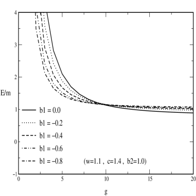
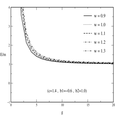
Figure 1: The total energy as a function of the Yukawa coupling constant $g$ with $m_{H}=0.35v$.

The existence of configurations with total energy $E_{\rm tot}/m<1$ shows that there is a stable soliton whose energy is at most $E_{\rm tot}$. Apparently a sizable Yukawa coupling $g$ is needed to obtain a stable soliton. However, as we will discuss later, our model is not reliable for such large Yukawa couplings because the Landau pole appears at an energy scale comparable to $1/w$.

In Fig. 2 we display the total energy as a function of the depth parameters $b_{1}$ and $b_{2}$, for various values of the Yukawa coupling constant $g$ and typical values of the remaining variational parameters $w$ and $c$.

         

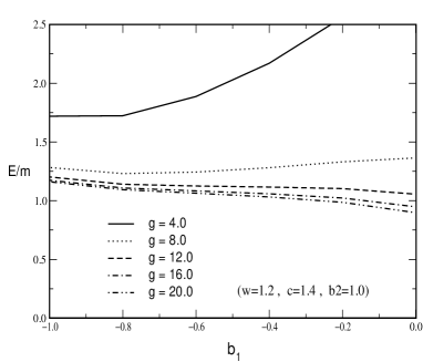
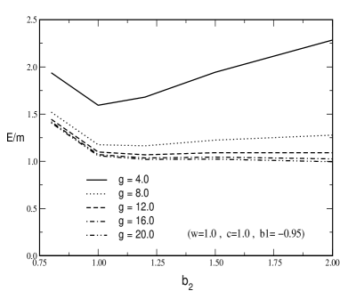
Figure 2: Total energy as a function of the depth parameters $b_{1}$ and $b_{2}$ with $m_{H}=0.35v$ and for various values of the Yukawa coupling constant $g$.

We observe a shallow local minimum in the vicinity of $b_{1}=-0.8$ for small and moderate values of $g$. However, at this minimum the total energy is larger than the mass $m$ of the free fermion. For larger $g$, we obtain a total energy less than $m$ for configurations with $b_{1}\approx 0$. Configurations with $b_{1}>0$ are more strongly bound, but the one fermion loop approximation fails for such configurations because the energy functional is not bounded from below (see Appendix C). We have therefore restricted the space of variational parameters to configurations for which the vacuum is stable to one loop.

We observe a similar behavior for $E_{\rm tot}$ as a function of $b_{2}$. There exists a local minimum for small and moderate $g$ that does not yield a bound soliton. For large $g$, a bound soliton seems possible if $b_{2}$ is big enough. In this case, the vacuum is stable at one loop for these values of the variational parameters. Note that when we find a marginally bound configuration, the vacuum polarization contribution to the energy $E_{\rm vac}$ tends to almost exactly compensate for the gain from binding a single level.

4.2 Comparison with the Derivative Expansion

In order to check our computation of the vacuum polarization energy, in particular the simplified treatment of the logarithmic divergence, we have compared our results with the derivative expansion. The relevant formulas for the derivative expansion are provided in Appendix C. Denoting by ${\cal E}_{\rm grad}$ the energy computed to second order in the derivative expansion as obtained from eq. (C.6), we display

$$\Delta_{1}\equiv\frac{{\cal E}_{\rm cl}+{\cal E}_{\rm vac}-{\cal E}_{\rm grad}}{{\cal E}_{\rm cl}+{\cal E}_{\rm vac}+{\cal E}_{\rm grad}}$$ (39)

as a function of the width parameter $w$. The other variational parameters are kept constant at $c=1.0$, $b_{1}=-0.4$ and $b_{2}=1.0$. Also, we consider various values for the coupling constant $g$.

Table 1: Comparison of the classical and renormalized vacuum polarization energy with the derivative expansion, cf. eq. (39).

$w$ 1.0 2.0 2.5 3.0 $g=\phantom{0}5.0$ –0.127 –0.024 –0.008 0.003 $g=10.0$ –0.240 –0.041 –0.013 0.005 $g=15.0$ –0.287 –0.048 –0.015 0.007 $g=20.0$ –0.308 –0.050 –0.015 0.006

Where the derivative expansion is valid we expect $\Delta_{1}$ to go to zero. From Table 1, we conclude that our calculation agrees with the derivative expansion at large $w$, where the derivative expansion becomes exact. In this region, the derivative expansion is a good check on our computation of the vacuum polarization energy. In particular, it checks our handling of renormalization, since renormalization effects are included in the derivative expansion in the standard way. On the other hand, it is clear from Table 1 that the second-order derivative expansion cannot be trusted for $w\approx 1.0$, i.e. for background configurations whose extension is close to the Compton wavelength of the fermion. One might imagine improving the derivative expansion by including the effect of an explicitly occupied level,

$$\Delta_{2}\equiv\frac{{\cal E}_{\rm tot}-{\cal E}_{\rm grad}}{{\cal E}_{\rm tot}+{\cal E}_{\rm grad}}$$ (40)

because the derivative expansion to $Q_{\rm vac}$, the topological charge, suggests that the background configuration carries fermion number regardless of the value for $w$. However, this modification does not give any better agreement at small $w$, as can be observed from Table 2. In general, the inclusion of the explicitly occupied level tends to change the sign of the relative deviation.

Table 2: Comparison of the total energy with the gradient expansion, cf. eq. (40).

$w$ 1.0 2.0 2.5 3.0 $g=\phantom{0}5.0$ 0.168 0.034 0.018 0.012 $g=10.0$ 0.257 0.056 0.029 0.019 $g=15.0$ 0.285 0.063 0.033 0.022 $g=20.0$ 0.297 0.066 0.034 0.023

4.3 The Landau Pole

From these studies one might conclude that a soliton takes over the role of the lightest fermion once the Yukawa coupling constant $g$ becomes large enough. At large $g$, the positive contribution to the total energy from ${\cal E}_{\rm cl}$ in eq. (37), which disfavors the soliton, decreases quickly for large $g$. However, for large couplings the model itself becomes ill-defined. Since the model is not asymptotically free, it has a Landau singularity in the ultraviolet, reflecting new dynamics at some cutoff scale. Thus the Landau pole sets a minimum distance scale below which the model is not consistent. Solitons that are large compared to this scale are relatively insensitive to the unknown dynamics at the cutoff scale, but solitons whose size is comparable to this scale cannot be trusted. In this section we will discuss the emergence of the Landau pole and estimate its effect on the vacuum polarization energy by comparing the present results with a calculation that removes this pole. Although this removal is somewhat ad hoc, it nevertheless provides some insight into the reliability of the computations in case of large $g$.

Denoting the Fourier transforms of $s(r)-1$ and $\vec{p}(r)$ by $h(\vec{q})$ and $\vec{p}(\vec{q})$, respectively, the contribution of the two-point function to the total energy can be written as

$$E_{2}=\frac{v^{2}}{2}\int\frac{d^{3}q}{(2\pi)^{2}}\left\{G_{h}^{-1}(-\vec{q}\,^{2})h(\vec{q})h(-\vec{q})+G_{p}^{-1}(-\vec{q}\,^{2})\vec{p}(\vec{q})\cdot\vec{p}(-\vec{q})\right\}$$ (41)

where

$$G_{h}^{-1}(q^{2}) = \frac{v^{2}}{2}\Bigg{\{}\left(q^{2}-m_{H}^{2}\right)\left(1+\frac{g^{2}}{4\pi^{2}}\right)$$ (42)

$$+\frac{g^{2}}{4\pi^{2}}6\int_{0}^{1}dx\left[m^{2}-x(1-x)q^{2}\right]\ln\frac{m^{2}-x(1-x)q^{2}}{m^{2}-x(1-x)m_{H}^{2}}\Bigg{\}}$$

$$G_{p}^{-1}(q^{2}) = \frac{v^{2}}{2}\Bigg{\{}q^{2}\left(1+\frac{g^{2}}{4\pi^{2}}\right)+\frac{g^{2}}{4\pi^{2}}\Bigg{[}6\int_{0}^{1}dx\left[m^{2}-x(1-x)q^{2}\right]\ln\frac{m^{2}-x(1-x)q^{2}}{m^{2}-x(1-x)m_{H}^{2}}$$ (43)

$$+2m^{2}\int_{0}^{1}dx\left[3\ln\left(1-x(1-x)\frac{m_{H}^{2}}{m^{2}}\right)-2\ln\left(1-x(1-x)\frac{q^{2}}{m^{2}}\right)\right]\Bigg{]}\Bigg{\}}$$

which includes classical, loop, and counterterm contributions. $G_{p}(q^{2})$ has a pole (the Landau ghost pole) at space-like momentum $-m_{G}^{2}$ with residue $Z_{G}$. The pole location is easily obtained numerically from the condition $G_{p}^{-1}(q^{2}=-m_{G}^{2})=0$. In the vicinity of $q^{2}\approx-m_{G}^{2}$ we have the expansion

$$G_{p}^{-1}(q^{2})=\frac{1}{Z_{G}}\left(q^{2}+m_{G}^{2}\right)+{\cal O}\left(q^{2}+m_{G}^{2}\right)^{2}$$ (44)

with

$$\frac{1}{Z_{G}} = \frac{\partial}{\partial q^{2}}G_{p}^{-1}(q^{2})\Big{|}_{q^{2}=-m_{G}^{2}}$$ (45)

$$= \frac{v^{2}}{2}\Bigg{\{}1-\frac{g^{2}}{4\pi^{2}}\Bigg{[}6\int_{0}^{1}dxx(1-x)\ln\frac{m^{2}+x(1-x)m_{G}^{2}}{m^{2}-x(1-x)m_{H}^{2}}$$

$$\hskip 85.35826pt-4\int_{0}^{1}dx\frac{x(1-x)}{m^{2}+x(1-x)m_{G}^{2}}\Bigg{]}\Bigg{\}}\ .$$

The existence of this pole yields an unphysical negative contribution to the total energy at large space-like momenta, or equivalently for narrow background field configurations. Based on the Källén-Lehmann representation for the two-point function, the authors of Ref. [16] suggested a procedure to eliminate the Landau pole while maintaining chiral symmetry. They replace eq. (41) with

$$\bar{E}_{2}=\frac{v^{2}}{2}\int\frac{d^{3}q}{(2\pi)^{2}}\Delta_{p}^{-1}(-\vec{q}\,^{2})\left\{h(\vec{q})h(-\vec{q})+\vec{p}(\vec{q})\cdot\vec{p}(-\vec{q})\right\}$$ (46)

where $\Delta_{p}(q^{2})=G_{p}(q^{2})-Z_{G}/(q^{2}+m_{G}^{2})$ removes the Landau pole. We can easily adopt this procedure since we have already extracted the loop and counterterm contributions from the two-point function in eq. (32). That is, we replace $E_{\rm cl}+E_{\rm ct}^{(2)}+E_{\rm l,ct}^{(4)}$ by $\bar{E}_{2}+E_{\rm cl}^{(3,4)}$ with

$$\frac{1}{m}E_{\rm cl}^{(3,4)}=\frac{\pi\mu_{H}^{2}}{2g^{2}}\int_{0}^{\infty}dxx^{2}\left\{\left[2(s-1)+(s-1)^{2}+\vec{p}\,^{2}\right]^{2}-4(s-1)^{2}\right\}\ .$$ (47)

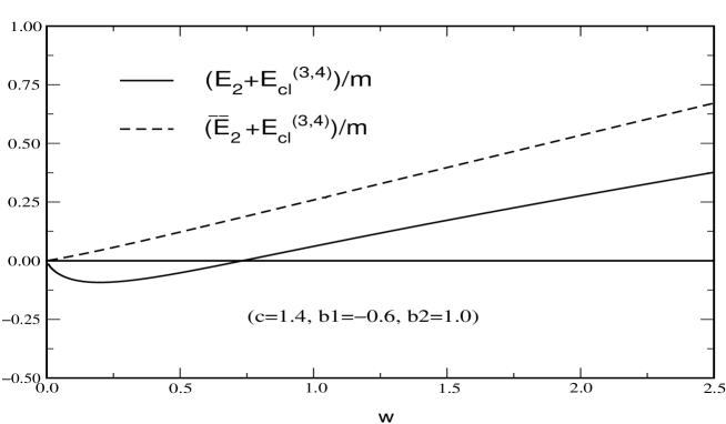
Figure 3: The Landau pole subtraction, for $m_{H}=0.35v$ and $g=12$.

In Fig. 3 we show the effect of this replacement as a function of the width parameter $w$ for $g=12$, which is in the region where a bound soliton can occur. For small $w$, we observe that the original computation, eq. (41), gives a negative contribution. However, for small $w$ there are only weakly bound states and the vacuum is almost undistorted. The classical energy is also small since $g$ is large. Hence the total energy is dominated by the renormalized Feynman diagram contribution $E_{\rm ct}^{(2)}+E_{\rm l,ct}^{(4)}$, which can be negative due to the Landau pole. Thus for small $w$ and large $g$, the Landau pole dominates the binding of the soliton, and, even worse, the total energy could be negative, reflecting an unphysical vacuum instability [6]. Using the above prescription to eliminate this pole, the total energy turns out to be positive for all values of $w$, so the instability is removed. As can be seen from Fig. 3, for sensible $w$ this prescription increases the total energy by about $0.25m$ for the parameters chosen, which unbinds the soliton. We conclude that the solitons found at large $g$ are principally bound by unphysical effects associated with the Landau singularity, and not by reliable dynamical properties of the model.

4.4 Scalar Backgrounds

We conclude the numerical analysis with a calculation of the total energy when only a scalar background field $s(r)$ is present. Our goal is a brief comparison with the results of Ref. [17], rather than a complete study. For $p\equiv 0$ the Dirac Hamiltonian is charge conjugation invariant. Hence the charge carried by the background field is zero and we must explicitly occupy the most strongly bound state. In Fig. 4 we show typical results of the numerical calculation for the total energy as a function of the coupling constant.

         

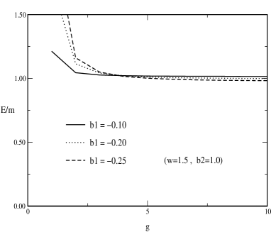
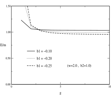
Figure 4: The total energy with only the scalar background as a function of the Yukawa coupling constant $g$ with $m_{H}=0.35v$. Note that the variational parameter $c$ is irrelevant without pseudoscalar fields.

The figure shows that a slightly bound soliton emerges even for modest values of the Yukawa coupling. Its energy is up to 5% less than that of a fermion in the background of the translationally invariant scalar field. In this case, the Landau ghost singularity in $G_{p}$ (cf. eq. (43)) is irrelevant and we may trust the calculation even for small $w$. Furthermore, the second-order derivative expansion deviates from the full calculation by only a fraction of a percent even at moderate values of the width parameter, $w\approx 1.5$. Plotting the results from the derivative expansion would yield indistinguishable curves in Fig. 4. Our approach thus confirms the findings of Ref. [17], which used the derivative expansion to find a slightly bound soliton.

5. Summary and Outlook

We have performed a quantitative search for Higgs solitons in a theory with chiral fermions. In the analogous model in one spatial dimension, such solitons exist and are strongly bound for a wide range of coupling constants. In three spatial dimensions, however, we did not find any region where the soliton binding was strong enough to be convincing. Twisted Higgs background fields do strongly bind a fermion level, but it is necessary to add the renormalized energy due to the distortion of the fermion vacuum. We have developed new methods to regularize, renormalize, and compute the corresponding vacuum polarization energy. In this model, we find that the vacuum polarization tends to cancel the contribution of the strongly bound fermion level. The total one-loop energy overcomes the classical energy only for large Yukawa couplings, where the theory has an unphysical Landau pole. Hence energetically favored Higgs solitons observed for large Yukawa couplings cannot be interpreted as reliable predictions of the model.

Nevertheless, these findings do not rule out the existence of Higgs solitons within the Standard Model. In particular, the inclusion of the gauge fields could be critical to soliton formation. This point of view is motivated by a number of considerations:

• Expanding the variational ansatz to include gauge fields can only decrease the energy of a configuration. In this respect, the $3+1$ dimensional model is different from the $1+1$ dimensional model where we did find a soliton, because in one dimension gauge fields do not add any new interactions.

• Gauge fields are essential to the anomaly arguments underlying the decoupling results.

• In the gauge theory, there is a sphaleron barrier with height $2\pi v/g_{W}$, where $v$ is the Higgs vacuum expectation value and $g_{W}$ is the gauge coupling. If the fermion has a Yukawa coupling $g_{F}$ such that its perturbative mass $g_{F}v$ is much larger than the sphaleron height, it has an unsuppressed decay mode over the sphaleron. Thus the ordinary fermion states are unstable and are nowhere to be found in the spectrum of the fermion Hamiltonian. The creation of a soliton state with mass below the sphaleron energy would allow the theory to remain gauge invariant after decoupling as required by [1].

Work is now underway to generalize this calculation to include the gauge fields.

Acknowledgments

We thank Vishesh Khemani for helpful discussions. E.F. and R.L.J. are supported in part by the U.S. Department of Energy (D.O.E.) under cooperative research agreement #DF-FC02-94ER40818. N.G. is supported by the U.S. Department of Energy (D.O.E.) under cooperative research agreement #DE-FG03-91ER40662 and H.W. is supported by the Deutsche Forschungsgemeinschaft under contracts We 1254/3-1,2.

Appendix A: Dirac equations

In this Appendix we present the first- and second-order Dirac equations used in Section 3 for fermions in a static background field in the spherical ansatz, eq. (15). In order to solve the Dirac equation, eqs. (16,17), we begin with spinors that are eigenstates of parity and total grand spin [5], where grand spin $\vec{G}$ is the sum of total angular momentum $\vec{j}=\vec{l}+\frac{1}{2}\vec{\sigma}$ and isospin ${\textstyle\frac{1}{2}}\vec{\tau}$. For a given grand spin quantum number $G$ with $z$-component $M$, we will find the bound state and scattering wavefunctions in terms of the spherical harmonic functions ${\cal Y}_{j,\ell}(\hat{x})$ with $j=G\pm\frac{1}{2}$ and $\ell=j\pm\frac{1}{2}$. These are two-component spinors in both spin and isospin space. In the following we will suppress the label $M$ for the $z$-component. While grand spin is conserved, the background field in eq. (15) mixes states with different total angular momentum $j$. For the channels with parity $\Pi=+(-)^{G}$, the spinor that diagonalizes eq. (16) reads

$$\Psi^{(+)}_{G}(\vec{x})=\pmatrix{ig_{1}(r){\cal Y}_{G+\frac{1}{2},G}(\hat{x})\cr f_{1}(r){\cal Y}_{G+\frac{1}{2},G+1}(\hat{x})}+\pmatrix{ig_{2}(r){\cal Y}_{G-\frac{1}{2},G}(\hat{x})\cr-f_{2}(r){\cal Y}_{G-\frac{1}{2},G-1}(\hat{x})}\ .$$ (A.1)

The spinor with opposite parity, $-(-)^{G}$, is parameterized as

$$\Psi^{(-)}_{G}(\vec{x})=\pmatrix{ig_{1}(r){\cal Y}_{G+\frac{1}{2},G+1}(\hat{x})\cr-f_{1}(r){\cal Y}_{G+\frac{1}{2},G}(\hat{x})}+\pmatrix{ig_{2}(r){\cal Y}_{G-\frac{1}{2},G-1}(\hat{x})\cr f_{2}(r){\cal Y}_{G-\frac{1}{2},G}(\hat{x})}\ .$$ (A.2)

Note that for convenience we have again suppressed both the grand spin and parity labels for the radial functions $g_{i}$ and $f_{i}$.

The matrix elements of the operator $\vec{\tau}\cdot\hat{x}$ between various ${\cal Y}_{jl}$ can be found in the literature [3]. Then the Dirac equation can be expressed as coupled first-order differential equations for the radial functions $g_{i}$ and $f_{i}$. In the $\Pi=+(-)^{G}$ parity channel, we have

$$0 = g_{1}^{\prime}-\frac{G}{r}g_{1}+(ms+\omega)f_{1}-\frac{mp}{2G+1}\left(g_{1}-2\sqrt{G(G+1)}g_{2}\right)$$

$$0 = g_{2}^{\prime}+\frac{G+1}{r}g_{2}-(ms+\omega)f_{2}+\frac{mp}{2G+1}\left(g_{2}+2\sqrt{G(G+1)}g_{1}\right)$$

$$0 = f_{1}^{\prime}+\frac{G+2}{r}f_{1}+(ms-\omega)g_{1}+\frac{mp}{2G+1}\left(f_{1}+2\sqrt{G(G+1)}f_{2}\right)$$

$$0 = f_{2}^{\prime}-\frac{G-1}{r}f_{2}-(ms-\omega)g_{2}-\frac{mp}{2G+1}\left(f_{2}-2\sqrt{G(G+1)}f_{1}\right)$$ (A.3)

where a prime indicates a derivative with respect to $r$. In the $\Pi=-(-)^{G}$ parity channel, we have

$$0 = g_{1}^{\prime}+\frac{G+2}{r}g_{1}-(ms+\omega)f_{1}-\frac{mp}{2G+1}\left(g_{1}-2\sqrt{G(G+1)}g_{2}\right)$$

$$0 = g_{2}^{\prime}-\frac{G-1}{r}g_{2}+(ms+\omega)f_{2}+\frac{mp}{2G+1}\left(g_{2}+2\sqrt{G(G+1)}g_{1}\right)$$

$$0 = f_{1}^{\prime}-\frac{G}{r}f_{1}-(ms-\omega)g_{1}+\frac{mp}{2G+1}\left(f_{1}+2\sqrt{G(G+1)}f_{2}\right)$$

$$0 = f_{2}^{\prime}+\frac{G+1}{r}f_{2}+(ms-\omega)g_{2}-\frac{mp}{2G+1}\left(f_{2}-2\sqrt{G(G+1)}f_{1}\right)\ .$$ (A.4)

We can use these differential equations to obtain the bound state solutions with $|\omega|<m$ using ordinary shooting methods. For a number of cases, we have verified the solutions numerically by diagonalizing eq. (16) in a spherical cavity [18]. As discussed in Section 3, we also require the second-order equations for either the upper ($g_{i}$) or lower ($f_{i}$) components of the Dirac spinor. These components will be collected into the matrix $F(r)H(kr)$ defined in eq. (18). In Section 3 we chose to work with the upper components only. Here we will discuss both upper and lower components, $F_{u}(k)$ and $F_{l}(k)$. Substituting this parameterization into the second-order equations for the upper or lower components of the Dirac equation and multiplying by the inverse of $H(kr)$ from the right, we obtain for the upper components in the channel with $\Pi=+(-)^{G}$

$$0=F_{u}^{\prime\prime}+\frac{2}{r}F_{u}^{\prime}\left[1+rL_{+}^{\prime}(kr)\right]-\frac{s^{\prime}}{s+\frac{\omega}{m}}\left[F_{u}^{\prime}+F_{u}L_{+}^{\prime}(kr)\right]+V(r,m)F_{u}$$ (A.5)

with $F=F_{u}$ entering eq. (20). The matrix $L_{+}(kr)$ is defined in eq. (22). For later convenience we have added the fermion mass $m$ as an argument of the potential matrix,

$$V_{11}(r,m) = -m^{2}\left[s^{2}+p^{2}-1\right]+\frac{G}{r}\frac{s^{\prime}}{s+\frac{\omega}{m}}-\frac{mp^{\prime}}{2G+1}-\frac{2}{r}\frac{(G+1)mp}{2G+1}+\frac{mp}{2G+1}\frac{s^{\prime}}{s+\frac{\omega}{m}}$$

$$V_{22}(r,m) = -m^{2}\left[s^{2}+p^{2}-1\right]-\frac{G+1}{r}\frac{s^{\prime}}{s+\frac{\omega}{m}}+\frac{mp^{\prime}}{2G+1}-\frac{2}{r}\frac{Gmp}{2G+1}-\frac{mp}{2G+1}\frac{s^{\prime}}{s+\frac{\omega}{m}}$$

$$V_{12}(r,m) = V_{21}(r,m)=\frac{2\sqrt{G(G+1)}}{2G+1}\left[mp^{\prime}+mp\left(\frac{1}{r}-\frac{s^{\prime}}{s+\frac{\omega}{m}}\right)\right]\ .$$ (A.6)

Similarly, we find the second-order equation for the lower components in the channel with $\Pi=+(-)^{G}$ is

$$0=F_{l}^{\prime\prime}+\frac{2}{r}F_{l}^{\prime}\left[1+rL_{-}^{\prime}(kr)\right]-\frac{s^{\prime}}{s-\frac{\omega}{m}}\left[F_{l}^{\prime}+F_{l}L_{-}^{\prime}(kr)\right]+W(r,m)F_{l}-\left[K,F_{l}\right]$$ (A.7)

where

$$W_{11}(r,m) = -m^{2}\left[s^{2}+p^{2}-1\right]-\frac{G+2}{r}\frac{s^{\prime}}{s-\frac{\omega}{m}}+\frac{mp^{\prime}}{2G+1}-\frac{2}{r}\frac{(G+1)mp}{2G+1}-\frac{mp}{2G+1}\frac{s^{\prime}}{s-\frac{\omega}{m}}$$

$$W_{22}(r,m) = -m^{2}\left[s^{2}+p^{2}-1\right]+\frac{G-1}{r}\frac{s^{\prime}}{s-\frac{\omega}{m}}-\frac{mp^{\prime}}{2G+1}-\frac{2}{r}\frac{Gmp}{2G+1}+\frac{mp}{2G+1}\frac{s^{\prime}}{s-\frac{\omega}{m}}$$

$$W_{12}(r,m) = W_{21}(r,m)=\frac{2\sqrt{G(G+1)}}{2G+1}\left[mp^{\prime}-mp\left(\frac{1}{r}+\frac{s^{\prime}}{s+\frac{\omega}{m}}\right)\right]\ .$$ (A.8)

In this case we have two different orbital angular momenta, leading to the commutator term $K=(1/r^{2})\,{\rm diag}\,\{(G+1)(G+2),G(G-1)\}$. Next we write down the differential equations in the channel with $\Pi=-(-)^{G}$ . Using definitions analogous to eqs. (18) we find for the upper components

$$0=F_{u}^{\prime\prime}+\frac{2}{r}F_{u}^{\prime}\left[1+rL_{-}^{\prime}(kr)\right]-\frac{s^{\prime}}{s+\frac{\omega}{m}}\left[F_{u}^{\prime}+F_{u}L_{-}^{\prime}(kr)\right]+W(r,-m)F_{u}-\left[K,F_{u}\right]$$ (A.9)

while the lower components obey

$$0=F_{l}^{\prime\prime}+\frac{2}{r}F_{l}^{\prime}\left[1+rL_{+}^{\prime}(kr)\right]-\frac{s^{\prime}}{s-\frac{\omega}{m}}\left[F_{l}^{\prime}+F_{l}L_{+}^{\prime}(kr)\right]+V(r,-m)F_{l}\ .$$ (A.10)

We must study the Born series in order to obtain the subtraction terms in eq. (31). We expand around the free solution,

$$F_{u}(r)=1+g_{s}F_{u}^{(1,0)}(r)+g_{p}F_{u}^{(0,1)}(r)+g_{s}^{2}F_{u}^{(2,0)}(r)+g_{p}^{2}F_{u}^{(0,2)}(r)+g_{s}g_{p}F_{u}^{(1,1)}(r)\ldots$$ (A.11)

and similarly for $F_{l}$. The expansion parameters $g_{p}$ and $g_{s}$ are defined by

$$\Phi(\vec{x})=v\left[1+g_{s}(s(r)-1)+ig_{p}\vec{\tau}\cdot\hat{x}\,p(r)\right]$$ (A.12)

where we have expanded the equations of motion and the potential matrices $V$ and $W$ in terms of the artificial coupling constants $g_{s}$ and $g_{p}$. Having obtained the second-order Dirac equations at the desired order in the couplings, we also expand the defining equation for the phase shifts, eq. (25), in these constants. Then, for example, $F^{(1,0)}$ and $F^{(0,1)}$ will contribute to $\delta^{(1)}_{G,p,\pi}$. However, we observe the relations

$$V^{n,2i+1}(r,m)\longleftrightarrow-V^{n,2i+1}(r,-m)\quad{\rm and}\quad W^{n,2i+1}(r,m)\longleftrightarrow-W^{n,2i+1}(r,-m)$$ (A.13)

when $\omega\longleftrightarrow-\omega$. As a result, once we sum over parity channels, the positive and negative energy pieces in the vacuum polarization energy calculation cancel for all odd powers of the pseudoscalar field. Of course, this cancellation just reflects parity invariance.

For scattering solutions, we have $|\omega|>m$ and hence the second-order equations are nonsingular as long as $|s|<1$. As explained in the main part of the paper we integrate these second-order equations from $r\to\infty$ to $r=0$. At $r\to\infty$ we have $s=1$ and commonly $s$ changes sign at some intermediate point, say $r_{0}$. For $\omega>0$ it is hence appropriate to use the second-order differential equations for the upper components, which will be the larger ones. Eventually, however, $s$ may become less than minus one. In that case we will have singularities when using the upper components. Then it would be more appropriate to employ the lower components as these will be the larger ones for $r<r_{0}$. For $\omega<0$ the situation is reversed. We therefore switch between these two components at $r=r_{0}$ using the first-order Dirac equations. In the parity $(-)^{G}$ channel the switch from upper to lower components is given by

$$F_{l} = \frac{-1}{\omega+ms}\sigma_{3}\left(F^{\prime}_{u}+F_{u}L_{+}^{\prime}+MF_{u}\right)H_{+}H_{-}^{-1}$$ (A.14)

$$F_{l}^{\prime} = -F_{l}L_{-}^{\prime}-\bar{M}F_{l}+(\omega-ms)\sigma_{3}F_{u}H_{+}H_{-}^{-1}\ .$$ (A.15)

In this case the upper components are obtained by integrating from infinity to $r_{0}$ and $F_{l}$ in eq. (A.15) is given by eq. (A.14). The matrices $M$ and $\bar{M}$ are defined by

$$M=\pmatrix{-\frac{G}{r}-\frac{mp}{2G+1}&2\frac{\sqrt{G(G+1)}}{2G+1}mp\cr 2\frac{\sqrt{G(G+1)}}{2G+1}mp&\frac{G+1}{r}+\frac{mp}{2G+1}}\quad{\rm and}\quad\bar{M}=\pmatrix{\frac{G+2}{r}+\frac{mp}{2G+1}&2\frac{\sqrt{G(G+1)}}{2G+1}mp\cr 2\frac{\sqrt{G(G+1)}}{2G+1}mp&-\frac{G-1}{r}-\frac{mp}{2G+1}}$$ (A.16)

where the Hankel function matrices $H_{\pm}$ are defined in eq. (19). The switch from lower to upper components is given by

$$F_{u} = \frac{1}{\omega-ms}\sigma_{3}\left(F^{\prime}_{l}+F_{u}L_{-}^{\prime}+\bar{M}F_{l}\right)H_{-}H_{+}^{-1}$$ (A.17)

$$F_{u}^{\prime} = -F_{u}L_{+}^{\prime}-MF_{l}-(\omega+ms)\sigma_{3}F_{u}H_{-}H_{+}^{-1}\ .$$ (A.18)

In the parity $-(-)^{G}$ channels the switch from upper to lower components is given by

$$F_{l} = \frac{1}{\omega+ms}\sigma_{3}\left(F^{\prime}_{u}+F_{u}L_{-}^{\prime}+NF_{u}\right)H_{-}H_{+}^{-1}$$ (A.19)

$$F_{l}^{\prime} = -F_{l}L_{+}^{\prime}-\bar{N}F_{l}-(\omega-ms)\sigma_{3}F_{u}H_{-}H_{+}^{-1}$$ (A.20)

with

$$N=\pmatrix{\frac{G+2}{r}-\frac{mp}{2G+1}&2\frac{\sqrt{G(G+1)}}{2G+1}mp\cr 2\frac{\sqrt{G(G+1)}}{2G+1}mp&-\frac{G-1}{r}+\frac{mp}{2G+1}}\quad{\rm and}\quad\bar{N}=\pmatrix{-\frac{G}{r}+\frac{mp}{2G+1}&2\frac{\sqrt{G(G+1)}}{2G+1}mp\cr 2\frac{\sqrt{G(G+1)}}{2G+1}mp&\frac{G+1}{r}-\frac{mp}{2G+1}}$$ (A.21)

and the transformation from lower to upper components is

$$F_{u} = \frac{-1}{\omega-ms}\sigma_{3}\left(F^{\prime}_{l}+F_{u}L_{+}^{\prime}+\bar{N}F_{l}\right)H_{+}H_{-}^{-1}$$ (A.22)

$$F_{u}^{\prime} = -F_{u}L_{-}^{\prime}-NF_{l}+(\omega+ms)\sigma_{3}F_{u}H_{+}H_{-}^{-1}\ .$$ (A.23)

Finally, we note that the required ratios of Hankel functions can also be expressed as rational functions

$$H_{+}H_{-}^{-1} = \frac{1}{k}\left[\sigma_{3}L_{-}^{\prime}+\frac{1}{r}\pmatrix{G+2&0\cr 0&G-1}\right]$$

$$H_{-}H_{+}^{-1} = \frac{1}{k}\left[-\sigma_{3}L_{-}^{\prime}+\frac{1}{r}\pmatrix{G&0\cr 0&G+1}\right]\ .$$ (A.24)

Appendix B: Fake Boson Field

In this Appendix, we describe the special treatment of the logarithmic divergence of Feynman diagrams. In particular we will explain and provide numerical evidence for the use of the simplified form in eqs. (31) and (33).

1. Discussion

In a fermion loop calculation, diagrams with one or two external lines are quadratically divergent and those with three or four are logarithmically divergent. Hence we will have to take $N_{\rm max}=4$ in eq. (3). Although we can straightforwardly compute the corresponding Born terms as in eqs. (28) and (29), the equivalent Feynman diagrams are difficult to compute numerically when the external fields are coordinate-dependent. All we really need to do, however, is to regulate the momentum integral in eq. (3) by subtracting an appropriate expression from the integrand and ensure that we add back in exactly the same quantity. The latter quantity should have a divergent piece that can easily be canceled by the counterterms. Boson loops have a much simpler divergence structure: the logarithmic divergence corresponds to a Feynman diagram that is only second order in the external lines. Higher-order boson loop diagrams are finite. We can therefore simplify the regularization of the logarithmic divergence of the fermion loop significantly by subtracting and adding back the contributions of an equivalent boson. This boson is completely artificial to the model so we will call it the “fake boson field.” We impose the condition that at one loop the fake boson model generates the same regulated logarithmic divergence as the original fermion loop. We then subtract the associated second-order Born phase shift from the fermion phase shifts and add it back in as a regulated Feynman diagram. By construction, its divergent piece is canceled by the counterterm contributions in eq. (3). This fake boson method does not give the full Feynman diagrams of the fermion loop, so the approach is not suitable to determine counterterm coefficients in a specified renormalization prescription. It can only be used once these coefficients are known. In our model we have uniquely determined the counterterms from the first- and second-order terms in the expansion of the fermion loop, which we computed exactly. We can then apply the fake boson method to the third- and fourth-order terms, which would otherwise be difficult to evaluate. We can extract the local piece of a Feynman diagram by setting the external momenta to zero. An expansion in the external momenta then shows that for a second-order boson diagram only this local piece diverges. We will identify the local piece in the second-order boson diagram as a “limiting function” to the the second-order Born approximation to the phase shift. This procedure provides the simplified expression used in eqs. (30)–(33).

2. Equivalent Boson

We begin by considering the second-order Born approximation to a boson loop. We consider the spherically symmetric problem

$$-\frac{d^{2}}{dr^{2}}u_{\ell}(r)+\left[\frac{\ell(\ell+1)}{r^{2}}+gV(r)\right]u_{\ell}(r)=k^{2}u_{\ell}(r)$$ (B.1)

discussed in Ref. [12]. The coupling constant $g$ is a bookkeeping device which at the end we will take to be unity. Solving for the complex function $\beta_{\ell}(k,r)$ in the ansatz $u_{\ell}(r)={\rm exp}(2i\beta_{\ell}(k,r))rh^{(1)}_{\ell}(kr)$ with the boundary conditions $\beta_{\ell}(k,\infty)=\beta^{\prime}_{\ell}(k,\infty)=0$ yields the phase shifts [12]

$$\delta_{\ell}(k)=-2{\rm Re}\beta_{\ell}(k,0)\ .$$ (B.2)

The differential equation for $\beta_{\ell}(k,r)$ is non-linear and the expansion $\beta_{\ell}(k,r)=g\beta^{(1)}_{\ell}(k,r)+g^{2}\beta^{(2)}_{\ell}(k,r)+\ldots$ yields the various orders of the Born series to the phase shifts $\delta^{(n)}_{\ell}=-2{\rm Re}\beta^{(n)}_{\ell}(k,0)$ by iteratively solving the differential equations for $\beta^{(n)}_{\ell}(k,r)$. $V(r)$ provides the source term for $\beta^{(1)}_{\ell}(k,r)$. Formally, the quadratically and logarithmically divergent contributions to the vacuum polarization energy are contained in

$$E^{(1)}_{\rm cas} = \int_{0}^{\infty}\frac{dk}{\pi}\sqrt{k^{2}+m^{2}}\frac{d}{dk}\sum_{\ell}(2\ell+1)\delta^{(1)}_{\ell}(k)$$

$$E^{(2)}_{\rm cas} = \int_{0}^{\infty}\frac{dk}{\pi}\sqrt{k^{2}+m^{2}}\frac{d}{dk}\sum_{\ell}(2\ell+1)\delta^{(2)}_{\ell}(k)\ .$$ (B.3)

Now let us consider two potentials, $V_{1}(r)$ and $V_{2}(r)$, which are related by

$$\int_{0}^{\infty}dr\,r^{2}V^{2}_{1}(r)=\int_{0}^{\infty}dr\,r^{2}V^{2}_{2}(r)$$ (B.4)

where we also allow for different masses $m_{1}$ and $m_{2}$ of the boson field. The dispersion relation $\omega=\sqrt{k^{2}+m_{i}^{2}}$ is the only place where a dependence on the mass appears since eq. (B.1) does not contain the mass parameter explicitly.

Since the logarithmically divergent counterterm only depends on the potential through the quantity $\int d^{3}xV(x)^{2}$, it will be identical for both potentials. Therefore the difference of the second-order Feynman diagrams

$$\Delta_{\rm F} = \frac{1}{(4\pi)^{2}}\int_{0}^{\infty}\frac{dq\,q^{2}}{(2\pi)^{2}}\tilde{V_{1}}(q)\tilde{V_{1}}(-q)\left[-2+\sqrt{1+\frac{4m_{1}^{2}}{q^{2}}}\,\ln\frac{\sqrt{1+\frac{4m_{1}^{2}}{q^{2}}}+1}{\sqrt{1+\frac{4m_{1}^{2}}{q^{2}}}-1}\right]$$ (B.5)

$$-\frac{1}{(4\pi)^{2}}\int_{0}^{\infty}\frac{dq\,q^{2}}{(2\pi)^{2}}\tilde{V_{2}}(q)\tilde{V_{2}}(-q)\left[-2+\sqrt{1+\frac{4m_{2}^{2}}{q^{2}}}\,\ln\frac{\sqrt{1+\frac{4m_{2}^{2}}{q^{2}}}+1}{\sqrt{1+\frac{4m_{2}^{2}}{q^{2}}}-1}\right]$$

will be finite. Here $\tilde{V_{i}}(q)$ denotes the Fourier transform of $V_{i}(r)$. Since we can identify orders in the Feynman diagrams with those in the Born series for the vacuum polarization energy, $\Delta_{\rm F}$ should be identical to

$$\Delta_{\rm V}=E^{(2)}_{{\rm cas,}1}-E^{(2)}_{{\rm cas,}2}$$ (B.6)

where the difference is to be taken under the integral in the second equation of (B.3). The second subscript, $i=1,2$, refers to the potential $V_{i}$. In Table B.1 we compare $\Delta_{\rm F}$ and $\Delta_{\rm V}$ for two Gaussian-type choices

$$V_{1}(r)=d^{2}{\rm e}^{-r^{2}/w^{2}}+2d{\rm e}^{-r^{2}/2w^{2}}\qquad{\rm and}\qquad V_{2}(r)=C{\rm e}^{-r^{2}/2w^{2}}\ .$$ (B.7)

Here $d$ and $w$ are variational parameters and the coefficient $C$ is fixed by eq. (B.4).

Table B.1: Comparison of second-order contributions to the vacuum polarization energy.

$d\,\,$ $w$ $m_{2}/m_{1}$ $\Delta_{V}\,$ $\Delta_{F}\,$ –2.0 2.0 1.0 0.088 0.087 –2.0 2.0 0.5 6.915 6.916 –2.0 2.0 2.0 –7.309 –7.312 2.0 0.8 1.0 0.010 0.010 2.0 1.5 1.0 0.023 0.023 3.0 2.0 1.0 0.011 0.011

We observe that the differences $\Delta_{V}$ and $\Delta_{F}$ agree within the numerical accuracy even though either of them may be quite large in magnitude, especially when the two masses are taken to be different. We conclude that we can subtract the second Born approximation and add back in the second-order Feynman diagram associated with bosonic fluctuations about $V_{1}$ to regulate the logarithmic divergences encountered in the study of any other problem with the same divergences. The method we employ in the Yukawa model is the generalization of this procedure to the case of fermions. Note that by considering the second-order Dirac equation (cf. Appendix A) the phase shift calculation in the Yukawa model is essentially that of a boson field with derivative interactions.

3. Limiting Function

Next we extract a local contribution containing the logarithmic divergence. We will manipulate this expression so that it can be substituted into the phase shift formula for the vacuum polarization energy. This procedure leads to further simplifications for evaluating the fermion vacuum polarization energy. Since these manipulations involve divergent objects they are not rigorous results. However, we will be able to verify their validity numerically for a specific background potentials. This check is sufficient to justify the use of these simplifications in the Yukawa model because we can always revert to that specific potential using the arguments of the previous subsection.

We formally identify the local contribution by setting the external momenta to zero in the second-order Feynman diagram

$$I_{\rm loc} = \frac{i}{2}\int d^{3}r\,V^{2}(r)\int\frac{d^{4}k}{(2\pi)^{4}}\left[k^{2}-m^{2}-i\epsilon\right]^{-2}$$ (B.8)

$$= \frac{-1}{8}\int_{0}^{\infty}dr\,r^{2}\,V^{2}(r)\int_{0}^{\infty}\frac{dk}{\pi}\sqrt{k^{2}+m^{2}}\frac{d}{dk}\left\{\frac{1}{m}\arctan\frac{m}{k}+\frac{k}{k^{2}+m^{2}}\right\}$$

where we have carried out finite $k_{0}$ and angular integrals. Nevertheless, these manipulations are formal since they involve the logarithmically divergent $k$-integral. However, so far we have only manipulated the integrand. It is worthwhile to note that the $k$ dependent function in the last integral equals that of the last term in eq. (31). We subtract the local contribution from the full second-order Feynman diagram, giving

$$\Delta E_{\rm F}^{(2)}=\frac{1}{(4\pi)^{2}}\int_{0}^{\infty}\frac{dq\,q^{2}}{(2\pi)^{2}}\tilde{V}(q)\tilde{V}(-q)\left[-2+\sqrt{1+\frac{4m^{2}}{q^{2}}}\,\ln\frac{\sqrt{1+\frac{4m^{2}}{q^{2}}}+1}{\sqrt{1+\frac{4m^{2}}{q^{2}}}-1}\right]$$ (B.9)

which, of course, is finite for the potentials of the type listed in eq. (B.7). Similarly we can define a finite second-order energy by subtracting the formal expression from the second Born approximant to the vacuum polarization energy

$$\Delta E_{\rm V}^{(2)}=\int_{0}^{\infty}\frac{dk}{\pi}\sqrt{k^{2}+m^{2}}\frac{d}{dk}\left[\left(\sum_{\ell}(2\ell+1)\delta^{(2)}(k)\right)-\delta^{(2)}_{\rm lim.~{}fct.}(k)\right]$$ (B.10)

where the limiting function is given by

$$\delta^{(2)}_{\rm lim.~{}fct.}(k)=-\frac{1}{8}\int_{0}^{\infty}dr\,r^{2}V^{2}(r)\left\{\frac{1}{m}\arctan\frac{m}{k}+\frac{k}{k^{2}+m^{2}}\right\}$$ (B.11)

In Table B.2 we compare $\Delta E_{\rm F}^{(2)}$ and $\Delta E_{\rm V}^{(2)}$ for the background potential $V_{1}(r)$ given in eq. (B.7). The particle in the loop of the local contribution does not need to have the same mass as that in the full Feynman diagram.

Table B.2: Comparison of the second-order Feynman diagram including the local subtraction with the corresponding expression for the vacuum polarization energy.

$d$ $w$ $m_{2}/m_{1}$ $\Delta E_{\rm F}^{(2)}\!\!$ $\Delta E_{\rm V}^{(2)}\!\!$ 2.0 0.8 1.0 0.001 0.001 2.0 1.5 1.0 0.002 0.002 3.0 2.0 2.0 0.113 0.112 1.0 1.5 0.8 0.069 0.069 1.0 1.5 1.2 –0.036 –0.036

Within the numerical accuracy we do not find any differences.

Appendix C: Derivative expansion

Using the techniques developed in Ref. [19] we compute the two leading orders of the derivative expansion for the fermion determinant

$$\Gamma(\Phi)=-i\,{\rm Tr}\,\ln\,\left\{i\partial\hskip-5.50003pt/-g\Phi_{5}\right\}\ .$$ (C.1)

First we compute the effective potential. In dimensional regularization,

$$V(\Phi)=\frac{2}{(4\pi)^{2}}\left[\frac{1}{\epsilon}-\gamma+\frac{3}{2}-\ln\,\frac{g^{2}\Phi^{2}}{4\pi\mu^{2}}\right]g^{4}\Phi^{4}$$ (C.2)

where $\mu$ is the scale introduced to render $g$ dimensionless in $d=4-2\epsilon$ dimensions. In order to extract the contribution with two derivatives acting on $\Phi$ we parameterize $\Phi=\Phi_{0}+\delta\Phi$ with $\Phi_{0}$ constant. Since

$$\Gamma(\Phi_{0}+\delta\Phi)=-V(\Phi_{0}+\delta\Phi)+\frac{1}{2}\Gamma_{\mu\nu}^{(2)}(\Phi_{0})\partial^{\mu}\delta\Phi\partial^{\nu}\delta\Phi+{\cal O}(\partial\delta\Phi)^{4}$$ (C.3)

it is sufficient to expand $\Gamma(\Phi_{0}+\delta\Phi)$ to quadratic order in both $\delta\Phi$ and the momentum of its Fourier transformation. Returning to configuration space this yields

$$\frac{i}{6}\int d^{4}x\int\frac{d^{4}q}{(2\pi)^{4}}\Bigg{\{}\frac{2}{(q^{2}-g^{2}\Phi_{0}^{2})^{2}}{\rm tr}_{F}\left(\partial_{\mu}\delta\Phi\partial^{\mu}\delta\Phi^{\dagger}\right)$$

$$\hskip 42.67912pt+\frac{1}{(q^{2}-g^{2}\Phi_{0}^{2})^{3}}\left[4q^{2}{\rm tr}_{F}\left(\partial_{\mu}\delta\Phi\partial^{\mu}\delta\Phi^{\dagger}\right)+4g^{2}{\rm tr}_{F}\left(\Phi_{0}^{\dagger}\partial_{\mu}\delta\Phi\Phi_{0}^{\dagger}\partial^{\mu}\delta\Phi\right)\right]\Bigg{\}}\ .\hskip 28.45274pt$$ (C.4)

Now we replace $\Phi_{0}$ by $\Phi$ and $\partial_{\mu}\delta\Phi$ by $\partial_{\mu}\Phi$ and treat the loop integral in dimensional regularization,

$$\frac{g^{2}}{(4\pi)^{2}}\int d^{4}x\left(\frac{1}{\epsilon}-\gamma-\frac{3}{2}-\ln\,\frac{g^{2}\Phi^{2}}{4\pi\mu^{2}}\right){\rm tr}_{F}\left(\partial_{\mu}\Phi\partial^{\mu}\Phi^{\dagger}\right)$$

$$\hskip 56.9055pt+\frac{1}{3}{\rm tr}_{F}\left(\partial_{\mu}\Phi\partial^{\mu}\Phi^{\dagger}-\frac{1}{|\Phi|^{2}}\Phi^{\dagger}\partial_{\mu}\Phi\Phi^{\dagger}\partial^{\mu}\Phi\right)\ .$$ (C.5)

Combining the expressions eq. (C.2) and (C.5) with the counterterms computed in Section 3 yields the final result for the derivative expansion up to second order,

$${\cal L}^{(2)} = \frac{g^{2}}{(4\pi)^{2}}\Big{\{}\left[c_{2}-\ln\,\frac{|\Phi|^{2}}{v^{2}}\right]{\rm tr}_{F}\left(\partial_{\mu}\Phi\partial^{\mu}\Phi^{\dagger}\right)$$ (C.6)

$$\hskip 56.9055pt+\frac{1}{3}{\rm tr}_{F}\left(\partial_{\mu}\Phi\partial^{\mu}\Phi^{\dagger}-\frac{1}{|\Phi|^{2}}\Phi^{\dagger}\partial_{\mu}\Phi\Phi^{\dagger}\partial^{\mu}\Phi\right)\Big{\}}$$

$$-\frac{g^{4}}{8\pi^{2}}(1+c_{0})\left(|\Phi|^{2}-v^{2}\right)^{2}-\frac{g^{4}}{16\pi^{2}}\left[|\Phi|^{4}-v^{4}-2|\Phi|^{4}\ln\,\frac{|\Phi|^{2}}{v^{2}}\right]$$

where

$$c_{0} = \frac{m_{H}^{2}}{4m^{2}}+\frac{3}{2}\int_{0}^{1}dx\,\ln\,\left[1-x(1-x)\frac{m_{H}^{2}}{m^{2}}\right]$$

$$c_{2} = 6\int_{0}^{1}dx\,x(1-x)\,\ln\,\left[1-x(1-x)\frac{m_{H}^{2}}{m^{2}}\right]\ .$$

We observe that for configurations with $|\Phi|^{2}>v^{2}$, the sum of the classical energy and the contribution computed from eq. (C.6) can become negative. Such configurations will destabilize the vacuum. Numerically, we have verified that this behavior also emerges in the full calculation for the vacuum polarization energy, which goes beyond the derivative expansion. Certainly this is an artifact of the one-loop approximation, implying that within this approximation we may not consider such configurations.

Bibliography

• [1] E. D’Hoker and E. Farhi, Nucl. Phys. B248 (1984) 59, Nucl. Phys. B248 (1984) 77.
• [2] E. Witten, Phys. Lett. B117 (1982) 324.
• [3] S. Kahana and G. Ripka, Nucl. Phys. A429 (1984) 462.
• [4] E. Farhi, N. Graham, R. L. Jaffe, and H. Weigel, Nucl. Phys. B585 (2000) 443; Phys. Lett. B475 (2000) 335.
• [5] R. Alkofer, H. Reinhardt, and H. Weigel, Phys. Rept. 265 (1996) 139; C. V. Christov et al., Prog. Part. Nucl. Phys. 37 (1996) 91; and references therein.
• [6] G. Ripka and S. Kahana, Phys. Rev.  D36 (1987) 1233.
• [7] I. Aitchison, C. Fraser, E. Tudor, and J. Zuk, Phys. Lett. B 165 (1985) 162.
• [8] R. Ball and H. Osborn, Nucl. Phys. B263 (1986) 245.
• [9] I. Adjali, I. J. Aitchison and J. A. Zuk, Phys. Lett. B256 (1991) 497; D. Diakonov, V. Y. Petrov and P. V. Pobylitsa, Nucl. Phys. B306 (1988) 809.
• [10] B. Kämpfer and H. Reinhardt, Annalen Phys.  1 (1992) 106.
• [11] J. Baacke, Z. Phys. C53 (1992) 402; J. Baacke and A. Sürig, Z. Phys. C73 (1997) 369
• [12] E. Farhi, N. Graham, P. Haagensen and R. L. Jaffe, Phys. Lett. B427 (1998) 334;
• [13] N. Graham and R. L. Jaffe, Nucl. Phys. B544 (1999) 432; Nucl. Phys. B549 (1999) 516.
• [14] J. Schwinger, Phys. Rev. 94 (1954) 1362;
• [15] E. Farhi, N. Graham, R. L. Jaffe, and H. Weigel, Nucl. Phys.  B595 (2001) 536.
• [16] J. Hartmann, F. Beck, and W. Benz, Phys. Rev. C50 (1994) 3088.
• [17] J. Bagger and S. Naculich, Phys. Rev. Lett. 67 (1991) 2252; Phys. Rev. D45 (1992) 1395; S. G. Naculich, Phys. Rev. D46 (1992) 5487.
• [18] R. Alkofer and H. Weigel, Comp. Phys. Comm. 82 (1994) 30.
• [19] I. Aitchison and C. Fraser, Phys. Lett. 146B (1984) 63; Phys. Rev. D31 (1985) 2605.