Abstract

We generalize the worldline variational approach to field theory by introducing a trial action which allows for anisotropic terms to be induced by external 4-momenta of Green’s functions. By solving the ensuing variational equations numerically we demonstrate that within the (quenched) scalar Wick-Cutkosky model considerable improvement can be achieved over results obtained previously with isotropic actions. In particular, the critical coupling associated with the instability of the model is lowered, in accordance with expectations from Baym’s proof of the instability in the unquenched theory. The physical picture associated with a different quantum mechanical motion of the dressed particle along and perpendicular to its classical momentum is discussed. Indeed, we find that for large couplings the dressed particle is strongly distorted in the direction of its four-momentum. In addition, we obtain an exact relation between the renormalized coupling of the theory and the propagator. Along the way we introduce new and efficient methods to evaluate the averages needed in the variational approach and apply them to the calculation of the 2-point function.

1 Introduction

Feynman’s variational method for evaluating functional integrals, well known in condensed matter physics [1], makes use of a trial action containing variational parameters. Even though the exact action of the theory under consideration can in general be quite complicated, the trial action itself can be at most quadratic in the degrees of freedom of the theory because the only functional integrals which can be performed analytically are Gaussian ones. Clearly this imposes a significant constraint so that one might at first sight suspect that such a variational method, even if valid in principle, is likely to be of limited use in practice. This turns out not to be the case, however: Feynman formulated the variational calculation on the level of a non-local action for the polaron, obtained after integrating out the phonon degrees of freedom. This non-locality, which is shared by the trial action used by him, introduces considerable freedom for the variational principle to work with and hence he obtained numerical results for, e.g. the polaron’s groundstate energy, which differed – for a very large range of coupling constants – from the exact ones by at most 2 % percent.

Encouraged by this success we have extended this method to relativistic field theory  [2] – [7] following the pioneering, but largely forgotten, work by K. Mano  [8]. In these investigations Feynman’s approach was applied to a relativistic scalar field theory of two fields $\varphi$ and $\Phi$ with Lagrangian (in Minkowski space)

$${\cal L}\>=\>\frac{1}{2}\left(\partial_{\mu}\Phi\right)^{2}-\frac{1}{2}M_{0}^{2}\Phi^{2}+\frac{1}{2}\left(\partial_{\mu}\varphi\right)^{2}-\frac{1}{2}m^{2}\varphi^{2}+g\,\Phi^{2}\varphi$$ (1.1)

where we refer to the light field $\varphi$ as “meson” and to the heavy one ($\Phi$) as “nucleon”. This theory is the Wick-Cutkosky model [9, 10] and is of interest as it models, in a rather rough fashion, a simplified nucleon-pion theory without the complications of spin and isospin (and chiral symmetry). Due to the close similarity to the polaron model (indeed, the dressed nucleon might be referred to as “relativistic polaron”, the only essential difference being the space-time dimensionality) one would expect the variational method to work equally well in this setting. Despite of this similarity, there are noticable qualitative differences: most importantly, while the polaron is a stable (quasi-) particle at all couplings, it turns out (see Refs. [2, 3]) that the variational equations of the Wick-Cutkosky model only have (real) solutions below a critical coupling of $\alpha_{c}\approx 0.815$, where

$$\alpha\>=\>{g^{2}\over 4\pi M^{2}}$$ (1.2)

is the dimensionless coupling constant and $M$ the physical mass associated with the field $\Phi$. The existence of a critical coupling is likely to be a remnant of the well-known instability of cubic scalar field theories [11].

There has been renewed interest in this theory and its instability in recent years. Ahlig and Alkofer [12] have analysed the stability of the model using Dyson-Schwinger equation methods and have found a critical coupling rather similar to the one mentioned above. Tjon and coworkers [13] have studied the theory (without the radiative corrections which are responsible for the instability) using Monte-Carlo techniques and have recently also alluded to evidence of a critical coupling [14]. It has also been suggested by these authors [15] that the apparent stability of the quenched theory below some critical coupling is a real effect and not just a byproduct of approximations [16]. In principle, the “true” $\alpha_{c}$ in the quenched theory could be found numerically by Monte-Carlo simulation similar to the way the true ground state energy of the polaron has been determined by stochastic methods [17]. Notwithstanding the interest in this critical coupling, we also note that there has been a great deal of interest in recent years in field theories with imaginary or negative coupling constants (which would lead to stability even for the unquenched theory) which, although they have non-hermitian Hamiltonians, are nevertheless argued to have a positive-definite spectrum by virtue of their PT-symmetry [18]. Finally, of course, there is continued interest in using this field theory as a vehicle for examining boundstate problems [19].

In recent applications we have treated a more realistic fermionic theory, viz. Quantum Electrodynamics, by worldline variational methods [20] and obtained a compact non-perturbative expression for the anomalous mass dimension. This shows that this approach successfully describes the short-distance singularities of relativistic quantum field theories. It is remarkable that at the same time the long-distance behaviour is also caught to a large extent as evidenced by the proper threshold behaviour of scattering amplitudes in the scalar model [4, 6] or the correct exponentiation of infrared singularities in QED [21].

Encouraging as these specific results are, one would like to assess the reliability of the variational results in general. There are two obvious ways one can do this: the approximation at the heart of Feynman’s variational calculation is the cumulant expansion and corrections can be systematically calculated, as was done for the polaron in Ref.  [22]. Alternatively, one can make use of more general trial actions, thus allowing the variational principle more freedom to work with. It is the latter course of action which we pursue here, concentrating for simplicity on the simple scalar field theory defined in Eq. (1.1) and considered in Refs. [2, 3]. The results presented there employed a number of different forms for the trial action, culminating in the most general (isotropic), non-local, quadratic trial action possible. It might seem, because the trial action is required to be quadratic, that it is hard to improve on this. However, as has been explored within the context of the polaron in Ref. [23], one can make use of the external direction provided by the particle’s four-momentum to construct more general, anisotropic, trial actions. For the polaron this extra freedom only yields marginally improved results due to the nonrelativistic nature of that problem [23]. One might expect however, and we shall indeed find, that significant improvements can be achieved in the present, relativistic, theory.

The organization of this paper is as follows. In the next Section, after briefly summarizing the essential details of the variational method (for more details, we refer the reader to Ref. [2]), we describe the anisotropic trial action and derive the relevant variational equations. In Sec. 3 we present numerical results and in Sec. 4 we conclude. Technical details are collected in five appendices.

2 The variational method

2.1 Feynman’s variational method applied to the Wick-Cutkosky model and the anisotropic trial action

In the polaron variational approach the key elements are

• The reduction of degrees of freedom by using the particle (“worldline”) representation and by integrating out the mesons/photons. For example, in the one-nucleon sector of the scalar theory defined by Eq. (1.1) this is achieved by using the Feynman-Schwinger representation (as well as neglecting the functional determinant if one is working in the quenched approximation)

  $$\frac{1}{-\partial^{2}-M_{0}^{2}+2g\varphi(x)+i0}\>=\>-\frac{i}{2\kappa_{0}}\int_{0}^{\infty}dT\>\exp\left[\frac{i}{2\kappa_{0}}\left(-\partial^{2}-M_{0}^{2}+2g\varphi(x)\right)\,T\,\right]\>.$$ (2.1)

  Here $\kappa_{0}$ is a free (positive) parameter which reparametrizes the proper time $T$ without affecting the physics . The exponential factor on the r.h.s. of Eq. (2.1) can be considered as a proper-time evolution operator and may be represented as a quantum mechanical path integral. With $\varphi(x)$ now being a c-number quantity the integration over the mesonic field can be performed resulting in an effective action for the four-dimensional trajectory $x(t)$ of the nucleon

  $$S[x] = \int_{t_{0}}^{t_{0}+T}dt\left(-\frac{\kappa_{0}}{2}\right)\dot{x}^{2}(t)-\frac{g^{2}}{2\kappa_{0}^{2}}\int_{t_{0}}^{t_{0}+T}dt_{1}\int_{t_{0}}^{t_{0}+T}dt_{2}\,\int\frac{d^{4}k}{(2\pi)^{4}}\>\frac{1}{k^{2}-m^{2}+i0}$$ (2.2)

  $$\hskip 142.26378pt\cdot\exp\left\{-ik\cdot\left[x(t_{1})-x(t_{2})\right]\,\right\}\>\equiv\>S_{0}+S_{1}\>.$$

  Here the starting time $t_{0}$ is free since only the proper time interval $T$ matters. Convenient choices are $t_{0}=0$ or $t_{0}=-T/2$.

• The use of the Feynman-Jensen variational principle

  $$\int{\cal D}x\,e^{iS_{t}}\,\exp\left[\,i\left(S-S_{t}\right)\,\right] \equiv \left(\int{\cal D}x\,e^{iS_{t}}\right)\,\cdot\,\langle\,\exp\left[i\left(S-S_{t}\right)\right]\,\rangle_{S_{t}}$$ (2.3)

  $$\simeq \left(\int{\cal D}x\,e^{iS_{t}}\right)\,\cdot\,\exp\left[\,i\langle\,S-S_{t}\,\rangle_{S_{t}}\,\right]\,,$$

  where $<\ldots>_{S_{t}}$ refers to averaging with weight function $e^{iS_{t}}$ (normalized to $<1>_{S_{t}}=1$) and $\>\simeq\>$ indicates equality at the stationary point of the r. h. s. under unrestricted variations of the trial action $S_{t}$.

• A quadratic two-time trial action

  $$S_{t}^{\rm iso\>\>(1)}\>=\>S_{0}+\frac{i\kappa_{0}^{2}}{2}\int_{t_{0}}^{t_{0}+T}dt_{1}dt_{2}\>f(t_{1}-t_{2})\>\Bigl{[}\>x(t_{1})-x(t_{2})\>\Bigr{]}^{2}\;\;\;,$$ (2.4)

  in which the non-quadratic terms in the true action $S$ are approximated by an even retardation function $f(\sigma)$. Since $t_{0}$ is arbitrary (proper time-translation invariance) this function can only depend on the time difference $\sigma=t_{1}-t_{2}$. Note that the true action as well as the trial action are invariant under a constant translation in $x$. Therefore one also could take

  $$S_{t}^{\rm iso\>\>(2)}\>=\>S_{0}-i\kappa_{0}^{2}\int_{t_{0}}^{t_{0}+T}dt_{1}dt_{2}\>g(t_{1}-t_{2})\>\dot{x}(t_{1})\cdot\dot{x}(t_{2})\>,$$ (2.5)

  because two integration by parts and neglect of boundary terms show that this is equivalent to Eq. (2.4) with $f(\sigma)=\ddot{g}(\sigma)$.

Being mainly interested in the on-shell-limit of the Green functions of the theory it is convenient to include the Fourier transform over the endpoints into the path integral (“momentum averaging” in the parlance of Ref.  [2]) and to consider

$$\tilde{S}[x]\>=\>p\cdot x\>+S[x]\>.$$ (2.6)

The nucleon’s propagator may be calculated from the generating functional and the worldline representation via

$$G_{2}(p)\>=\>\frac{1}{2i\kappa_{0}}\>\int_{0}^{\infty}dT\>\exp\left[\frac{iT}{2\kappa_{0}}(p^{2}-M_{0}^{2})\right]\>\cdot\>\underbrace{{\int{\cal D}{\tilde{x}}\>e^{i\tilde{S}[x]}\over\int{\cal D}{\tilde{x}}\>e^{i\tilde{S}_{0}[x]}}}_{=:g_{2}(p,T)}\;\;\;.$$ (2.7)

Note that we have normalized the functional measure by dividing by the path integral involving the free action $S_{0}$ (i.e. Eq. (2.6) with $g=0$). As mentioned, the path integrals in Eq. (2.7) include an integral over the endpoint $x$ – hence the tilde over the $x$.

The variational approximation to this propagator, making use of Jensen’s stationary principle, has the form (2.7) but with

$$g_{2}(p,T)\>\simeq\>g_{2}^{\rm var}(p,T)\>=\>{\int{\cal D}{\tilde{x}}\>e^{i\tilde{S}_{t}[x]}\over\int{\cal D}{\tilde{x}}\>e^{i\tilde{S}_{0}[x]}}\,\exp\left[\,i\,{\int{\cal D}{\tilde{x}}\>(\tilde{S}[x]-\tilde{S}_{t}[x])\;e^{i\tilde{S}_{t}[x]}\over\int{\cal D}{\tilde{x}}\>e^{i\tilde{S}_{t}[x]}}\,\right]\;\;.$$ (2.8)

Of course, when the extended trial action $\tilde{S}_{t}$ equals $\tilde{S}$ this expression gives the exact propagator in Eq. (2.7). On the other hand, as long as $\tilde{S}_{t}$ is quadratic in $x(t)$, all functional integrals appearing in Eq. (2.8) may be performed analytically. The most general linear + quadratic isotropic trial action, respecting symmetries such as translational invariance, may be written as

$$\tilde{S}_{t}^{iso}[x]\>=\>\tilde{\lambda}\,p\cdot x+S_{t}^{\rm iso}$$ (2.9)

where $\tilde{\lambda}$ is an additional variational parameter. Note that the structure of the linear term is basically fixed by requiring that the action is a scalar and by time translation invariance: there is only one additional four-vector, the external momentum $p$, with which the velocity four-vector can be contracted and any modification of the free term $p\cdot x=p\cdot\int dt\,v(t)$ can only be done by multiplication with a constant, but not with a function of the proper time. In contrast, the retardation functions $f$ or $g$ in the quadratic term must be functions of the time difference $\sigma=t_{1}-t_{2}$.

The key to the success of Feynman’s variational method is that the different functional dependence on the path $x(t)$ in the exact action in Eq. (2.6) as compared to the trial action in Eq. (2.4) can be compensated for by the variational retardation function $f(\sigma)$. For example, in the path integral in Eq. (2.7) contributions from $[x(t_{1})-x(t_{2})]^{2}\approx 0$ are greatly enhanced because of the UV divergence in the interacting part of the action Eq. (2.6). In the path integral in Eq. (2.8) the equivalent enhancement is provided by a divergence of $f(\sigma)$ as $\sigma\rightarrow 0$. Similarly, infrared physics is simulated by the large-$\sigma$ behaviour of this function. However, in general it is to be expected that in the functional integral over $\,\exp(iS[x])\,$ paths which contain segments $x_{\mu}(t_{1})-x_{\mu}(t_{2})$ which are parallel to the momentum $p_{\mu}$ will receive a different weighting to those containing segments which are perpendicular to $p_{\mu}$. Because $f(\sigma)$ is scalar, the trial actions  (2.4, 2.5) cannot differentiate between these two. Rather, the behaviour of the retardation function $f(\sigma)$ will encapsulate some compromise of this directional information.

The situation is different, however, if we generalize the trial action by explicitly making use of the external vector $p_{\mu}$. The most general covariant, quadratic, anisotropic trial action may be written as

$$S_{t}^{\rm aniso\>1} = S_{0}+\frac{i\kappa_{0}^{2}}{2}\,\int_{t_{0}}^{t_{0}+T}dt_{1}dt_{2}\;\left[\,f_{L}(\sigma){p^{\mu}p^{\nu}\over p^{2}}+f_{T}(\sigma)\left(g^{\mu\nu}-{p^{\mu}p^{\nu}\over p^{2}}\right)\,\right]$$ (2.10)

$$\hskip 113.81102pt\cdot\biggl{[}\,x_{\mu}(t_{1})-x_{\mu}(t_{2})\biggr{]}\>\biggl{[}x_{\nu}(t_{1})-x_{\nu}(t_{2})\,\biggr{]}\;\;\;.$$

In this action we now have two independent retardation functions $f_{T}(\sigma)$ and $f_{L}(\sigma)$ and we shall show, in the following, that these indeed encode just that directional information in the functional integral which we have discussed above. Equivalently, just as in the isotropic case (i.e. Eq. (2.5)), one could take

$$S_{t}^{\rm aniso\>2}\>=\>S_{0}-i\kappa_{0}^{2}\,\int_{t_{0}}^{t_{0}+T}dt_{1}dt_{2}\;\left[\,g_{L}(\sigma){p^{\mu}p^{\nu}\over p^{2}}+g_{T}(\sigma)\left(g^{\mu\nu}-{p^{\mu}p^{\nu}\over p^{2}}\right)\,\right]\,\dot{x}_{\mu}(t_{1})\,\dot{x}_{\nu}(t_{2})\>\\$$ (2.11)

instead.

2.2 Mano’s equation and functional averages

In Appendix B it is detailed how the averages required in Eq. (2.8) may be calculated easily by a method which is more transparent and efficient than the Fourier series expansion used in Ref. [2]. In particular, Eq. (B.20) demonstrates that all trial actions may be written as

$$\tilde{S}_{t}[v]\>=\>-\frac{\kappa_{0}}{2}\,(v|A|v)+(b|v)$$ (2.12)

if expressed in terms of velocities $v$. Allowing for a Lorentz structure of $A$, i.e. $(v|A|v)\equiv(v_{\mu}|A^{\mu\nu}|v_{\nu})$, this is obviously the most general linear + quadratic trial action. In principle one could work out the required averages with this trial action and let the variational principle determine the form of $A$ and $b$. That this indeed leads to an anisotropic trial action is sketched in Appendix C. However, since there is only one four-vector available for the 2-point function, namely the external momentum $p$, it is clear that $b$ must be proportional to $p$ and that $A$ must have the decomposition (B.19), which reflects the Lorentz structure of the retardation functions in Eqs. (2.10, 2.11).

In the following we will only consider the limit of the 2-point function where $p^{2}\to M^{2}$, i.e. the on-mass-shell limit. It is well known [24] that in order to obtain the pole and the residue of the nucleon propagator

$$G_{2}(p)\>\longrightarrow\>\frac{Z}{p^{2}-M^{2}+i0}\>,$$ (2.13)

the proper time $T$ has to tend to infinity. To obtain the physical mass in terms of the bare mass only the leading large-$T$ term in the exponential of $g_{2}$ is of relevance (see Eq. (D.16) of Appendix D). Performing the $T$-integration in Eq. (2.7) and setting $p^{2}=M^{2}$ gives

$$M_{0}^{2}\>=\>(2\lambda-\lambda^{2})M^{2}-2(\Omega+V)\>.$$ (2.14)

This equation, whose content is discussed in detail below, was termed ‘Mano’s equation’ in Ref. [2]. There it was also shown that for fixed physical mass $M$ (and fixed UV regulator) the variational principle in fact provides a lower bound on the exact bare mass, i.e.

$$M_{0}^{2}({\rm exact})\>\geq\>M_{0}^{2}\,\left({\rm Eq.}~{}(\ref{eq: Mano})\right)\;\;\;.$$ (2.15)

The parameter $\lambda$ in Mano’s equation (2.14) is related to the original variational parameter $\tilde{\lambda}$ by

$$\lambda\>=\>\frac{\tilde{\lambda}}{A_{L}(0)}\>.$$ (2.16)

As shown in Eq. (D.8) those averages not involving the coupling $\alpha$ are contained in the ‘kinetic term’ $\Omega$, which in $d$ dimensions is given by

$$\Omega[A_{T},A_{L}]\>=\>\frac{1}{d}\Omega[A_{L}]+{d-1\over d}\,\Omega[A_{T}]\;\;\;,$$ (2.17)

with

$$\Omega[A_{L,T}]\>=\>{d\kappa_{0}\over 2i\pi}\int_{0}^{\infty}dE\>\left[\log A_{L,T}(E)\>+\>{1\over A_{L,T}(E)}\>-\>1\right]\;\;\;.$$ (2.18)

Note that when $A_{T}=A_{L}$ this reduces to the isotropic result and that the factor $d-1$ in front of the first term arises because in $d$ dimensions there are $d-1$ dimensions transverse to $p_{\mu}$. From Eqs. (D.10, D.11) it is seen that the transverse and longitudinal profile functions $A_{L,T}$ are essentially the cosine transforms of the transverse and longitudinal retardation functions, respectively. Since $\log A+1/A-1$ is positive for $A>0$ the kinetic term provides the restoring force to balance the attractive interaction.

The ‘potential’ term, essentially the average of the interaction dependent part of the action, is given by Eq. (D.15) which in $d=4$ dimensions reads

$$V = -\frac{g^{2}}{8\pi^{2}}\,\int_{0}^{\infty}d\sigma\,\int_{0}^{1}du\>\Biggl{\{}{F_{LT}^{3/2}(u,\sigma)\over\mu_{L}^{2}(\sigma)}\>\exp\left[-{i\over 2\kappa_{0}}\left(m^{2}\mu_{L}^{2}(\sigma){1-u\over u}+{\lambda^{2}M^{2}\sigma^{2}\over\mu_{L}^{2}(\sigma)}u\right)\right]$$ (2.19)

$$\hskip 113.81102pt-\>{1\over\sigma}\>\exp\left[-{i\over 2\kappa_{0}}m^{2}\sigma{1-u\over u}\right]\Biggr{\}}\>-\>{g^{2}\over 8\pi^{2}}\log{\Lambda^{2}\over m^{2}}.$$

In addition, we have used a Pauli-Villars regulator as in Ref. [2] to make the proper time integral convergent for small $\sigma$. As in Refs. [2, 3] the divergent logarithm on the right hand side will be taken over to the left hand side of Eq. (2.14), with the replacement of $M_{0}^{2}$ by the finite

$$M_{1}^{2}\>=\>M_{0}^{2}-{g^{2}\over 4\pi^{2}}\log{\Lambda^{2}\over m^{2}}\>.$$ (2.20)

The essential new element in Eq. (2.19) as compared to the isotropic case is the appearance of the anisotropy factor

$$F_{LT}(u,\sigma)\>=\>\left[\,1+\left({\mu_{T}^{2}(\sigma)\over\mu_{L}^{2}(\sigma)}-1\right)u\,\right]^{-1}\;\;\;.$$ (2.21)

Also, note that there is now one ‘pseudotime’ $\mu^{2}(\sigma)$ for each of $A_{L,T}(E)$:

$$\mu^{2}_{L,T}(\sigma)\>=\>{4\over\pi}\int_{0}^{\infty}{dE\over E^{2}}\>{\sin^{2}{E\sigma\over 2}\over A_{L,T}(E)}\;\;\;.$$ (2.22)

This function was named as such in Ref. [2] because, as can be seen rather straightforwardly from Eq. (2.22), it is proportional to $\sigma$ ($\sigma>0$) for small $\sigma$ as well as for large $\sigma$ (and, indeed, is equal to $\sigma$ when the interaction is turned off, i.e. when $A(E)=1$). Actually, these pseudotimes also have a direct physical interpretation: Let us consider, initially, the average separation $x(t_{1})-x(t_{2})$ when weighted with the exponential of the trial action. Using Eqs. (B.30, D.12) this is easily calculated and one obtains

$$\langle\,x^{\mu}(t_{1})-x^{\mu}(t_{2})\,\rangle_{\tilde{S}_{t}}\>=\>-\frac{a_{1}^{\mu}}{\kappa_{0}}\>\>\stackrel{{\scriptstyle T\to\infty}}{{\longrightarrow}}\>\>{\lambda p^{\mu}\over\kappa_{0}}\;\sigma\;\;\;.$$ (2.23)

The meaning of this expression is clear: the average (four-) displacement that the nucleon undertakes in the proper time interval $\sigma=t_{1}-t_{2}$ is given by its (four-) velocity $\cdot$ $\sigma$. It is natural then to view $\kappa_{0}/\lambda$ as an effective mass . That this interpretation is not at all unreasonable was seen for the 3-dimensional polaron problem discussed in Ref. [23], where the variational equations for $\lambda$ directly lead to this result.

It is very instructive to consider now the mean square displacement. With Eq. (D.13) one obtains

$$\langle\,\left[x^{\mu}(t_{1})-x^{\mu}(t_{2})\right]\,\left[x^{\nu}(t_{1})-x^{\nu}(t_{2})\right]\,\rangle_{S_{t}}\>=\>\frac{1}{\kappa_{0}^{2}}a_{1}^{\mu}a_{1}^{\nu}-\frac{i}{\kappa_{0}}a_{2}^{\mu\nu}\>\>\stackrel{{\scriptstyle T\to\infty}}{{\longrightarrow}}\>\>\frac{\lambda^{2}p^{\mu}p^{\nu}}{\kappa_{0}^{2}}\sigma^{2}-\frac{i}{\kappa_{0}}\left(\mu^{2}(\sigma)\right)^{\mu\nu}\>.$$ (2.24)

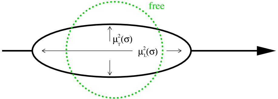
Figure 1: The physical interpretation of the pseudotimes $\mu_{L,T}(\sigma)$. The dotted circle denotes the noninteracting particle with quantum mechanical uncertainty in $\langle x^{2}\rangle$ given by Brownian motion alone.

The first term is again the contribution from the straight line (i.e. classical) motion. The last term characterizes both the quantum mechanical deviations from this as well as the ‘jiggling’ the nucleon experiences because of the constant emission and re-absorption of the pions. For example, as mentioned above the pseudotimes reduce to $\sigma$ and $\lambda=1$ when the interactions are turned off. In this case the first term in Eq. (2.24) represents a constant drift and the second just corresponds to the result well known from Brownian motion that the mean square distance (in each direction) grows linearly with Euclidean time (see footnote 2). Turning on the interactions modifies this Brownian motion, and since

$$\left(\mu^{2}(\sigma)\right)^{\mu\nu}\>=\>\mu^{2}_{L}(\sigma)\,\frac{p^{\mu}p^{\nu}}{p^{2}}+\mu^{2}_{T}(\sigma)\left(g^{\mu\nu}-\frac{p^{\mu}p^{\nu}}{p^{2}}\right)$$ (2.25)

this modification may be different in the longitudinal and transverse directions.

The results are summarized in the cartoon in Fig. 1, anticipating the numerical results from Section 3. Note that the possibility of distortion in the longitudinal direction is only present because the trial action has been allowed to be anisotropic. It is shown in Appendix C that for nonvanishing momentum $p$ the variational principle, if given sufficient freedom, demands such a structure.

2.3 The variational equations

By demanding that the independent variation of Mano’s equation (ie. Eq. (2.14)) with respect to the parameter $\lambda$ and the profile functions $A_{T}(E)$ and $A_{L}(E)$ must vanish, we obtain the variational equations for these functions. Since a numerical solution is only feasible in Euclidean space we choose $\kappa_{0}=i\kappa_{E}$. After some work one obtains

$${1\over\lambda}\>=\>1\>+\>{g^{2}\over 8\pi^{2}}\,\frac{1}{\kappa_{E}}\int_{0}^{\infty}d\sigma{\sigma^{2}\over\mu_{L}^{4}(\sigma)}\int_{0}^{1}du\>u\>F_{LT}^{3/2}(u,\sigma)\>\cdot e(u,\sigma)$$ (2.26)

$$A_{T}(E) = 1+\frac{8}{3\kappa_{E}E^{2}}\,\int_{0}^{\infty}d\sigma\>\frac{\delta V}{\delta\mu^{2}_{T}(\sigma)}\,\sin^{2}{E\sigma\over 2}$$

$$\frac{\delta V}{\delta\mu^{2}_{T}(\sigma)} = {3g^{2}\over 16\pi^{2}}\,\frac{1}{\mu_{L}^{4}(\sigma)}\int_{0}^{1}du\>u\,F_{LT}^{5/2}(u,\sigma)\>\cdot e(u,\sigma)$$ (2.27)

$$A_{L}(E) = 1+\frac{8}{\kappa_{E}E^{2}}\,\int_{0}^{\infty}d\sigma\>\frac{\delta V}{\delta\mu^{2}_{L}(\sigma)}\,\sin^{2}{E\sigma\over 2}$$

$$\frac{\delta V}{\delta\mu^{2}_{L}(\sigma)} = {g^{2}\over 16\pi^{2}}\frac{1}{\mu_{L}^{4}(\sigma)}\int_{0}^{1}du\>u\,F_{LT}^{3/2}(u,\sigma)\,\left(1-\frac{1}{\kappa_{E}}{\lambda^{2}M^{2}\sigma^{2}\over\mu_{L}^{2}(\sigma)}u\right)\>\cdot e(u,\sigma)$$ (2.28)

where

$$e(u,\sigma)\>\equiv\>\exp\left[\,-\frac{1}{2\kappa_{E}}\left(m^{2}\mu_{L}^{2}(\sigma)\frac{1-u}{u}+\frac{\lambda^{2}M^{2}\sigma^{2}}{\mu_{L}^{2}(\sigma)}u\right)\,\right]\>.$$ (2.29)

Note that the compact form of the last variational equation results from an appropriate integration by parts in $u$. Neither Eq. (2.27) nor Eq. (2.28) reduce to the variational equation for the isotropic profile function given in Sec. IV. C of Ref. [2] for $F_{LT}=1$ because the anisotropy factor $F_{LT}$ has been varied as well. However, both equations become identical when $M=0$ and $F_{LT}=1$. This just corresponds to the fact that when the momentum $p_{\mu}$ vanishes (hence $p^{2}=-M^{2}=0$) there is no source of anisotropy and hence no need for separate retardation functions in the longitudinal and transverse directions. In this case one also deduces from Eqs. (2.28) and (2.26) that $\lambda A(0)=1$, i.e. the original variational parameter $\tilde{\lambda}$ in the trial action (2.9) decouples and is unaffected by the interaction.

Finally, by comparison with Eq. (D.10) one also sees that the retardation functions defined in Eq. (2.10) are essentially the variational derivatives of the ‘potential’

$$f^{\rm var}_{L,T}(\sigma)\>=\>\frac{c_{L,T}}{\kappa_{E}^{2}}\,\frac{\delta V}{\delta\mu^{2}_{L,T}(\sigma)}\>,\>\>\>\>c_{L}\>=\>1\>,\>\>\>\>c_{T}\>=\>\frac{1}{3}\>.$$ (2.30)

2.4 The residue

For completeness we also evaluate the residue of the propagator in Eq. (2.13). This requires the calculation of the next-to-leading terms in the large-$T$ limit. As shown in Appendix D.2 only the interaction gives a ${\cal O}(T^{0})$-contribution to $\>\log g_{2}(p,T)\>$. Therefore following Sec. V. A in Ref. [3] and using Eq. (D.23) we easily obtain in $d=4$ Euclidean dimensions

$$Z\>=\>\frac{1}{\lambda}\,\exp\left[\,-\frac{g^{2}}{8\pi^{2}}\,\frac{1}{\kappa_{E}}\,\int_{0}^{\infty}d\sigma\,\frac{\sigma}{\mu_{L}^{2}(\sigma)}\int_{0}^{1}du\>F_{LT}^{3/2}(u,\sigma)\cdot e(u,\sigma)\,\right]\>\equiv\>\frac{N}{\lambda}\>.$$ (2.31)

As in Ref. [3], the variational equation (2.26) for $\lambda$ has been used to simplify the denominator of this expression. It is also easily seen that $Z$ does not depend on the value of $\kappa_{E}$.

Apart from the obvious modifications due to the anisotropic trial action and the general reparametrization gauge $\kappa_{E}\neq 1$, Eq. (2.31) differs from the result obtained in Ref. [3] by the absence of the factor $N_{0}=\exp[-\log A(0)+1-1/A(0)]$. As seen in Eq. (65) of Ref. [3] this factor had its origin in a ${\cal O}(1/T)$-correction to the kinetic term $\Omega$ which does not occur in the present formulation where an even, time-translation invariant retardation function (or equivalently, an even profile function $A(t-t^{\prime})$) has been employed throughout. The discrepancy is explained by recalling that – for practical reasons – the previous trial action was taken as a quadratic, diagonal form in Fourier space (see Eqs. (48) - (51) in Ref. [2]). After transforming back to $x$-space it may be seen that this form also contains terms which are not invariant under time translations. The present formulation therefore not only respects this obvious symmetry of the action but also eliminates the spurious and awkward $N_{0}$-term : after absorbing $A(0)$ in the variational parameter $\lambda$, it does not appear explicitly anymore, neither in the pole mass nor in the residue of the propagator.

2.5 The effective coupling

Finally, although it is beyond the scope of this paper to discuss the vertex function in general (for the isotropic trial actions this was done in Ref. [5]), it is rather straightforward to derive the effective coupling of the theory (i.e. the value of the vertex function at $q^{2}=0$) for an arbitrary trial action.

We start with the (exact) worldline representation of the untruncated 3-point function, which is closely related to the corresponding expression for the propagator, i.e. Eq. (2.7). The only difference is an additional plane wave $e^{iq\cdot x(\tau)}$ for the external pion with (outgoing) momentum $q^{\mu}$ and an integral over the proper time $\tau$ at which the pion couples to the nucleon’s worldline:

$$G_{2,1}(p,p^{\prime}=p-q)\,=\,{\rm const.}\>\int_{0}^{\infty}dT\exp\left[-{i\,T\over 2\kappa_{0}}M_{0}^{2}\right]\int{\cal D}\tilde{x}\>e^{-ip^{\prime}\cdot x}\left[g\int_{0}^{T}d\tau\>e^{iq\cdot x(\tau)}\right]e^{i\tilde{S}[x]}\;\;.$$ (2.32)

For $q^{\mu}=0$ the integral over the time $\tau$ just provides a factor of $T$, while the rest of the integrand is the same as the one for the propagator in Eq. (2.7). We therefore obtain

$$G_{2,1}(p,p)\>=\>2\,g\,{\partial\over\partial M_{0}^{2}}\>G_{2}(p)\;\;,$$ (2.33)

where the normalization has been fixed so that the correct free limit is obtained (see Ref. [5]; the factor $2$ arises because of the definition of the coupling in Eq. (1.1) without a factor $1/2!$) and we have made use of the fact that the only dependence on the bare mass enters through the explicit exponential factor shown in Eq. (2.32). One merely has to truncate the external legs off $G_{2,1}(p,p^{\prime})$ and multiply by the residue $Z$ in order to obtain the vertex function. At $q_{\mu}=0$ this defines the effective coupling $2\,g_{\rm phys}$. Hence the physical coupling of the theory and the propagator are related by the (exact) relation

$$g_{\rm phys}\>=\>-\,g\,Z\,{\partial\over\partial M_{0}^{2}}\>G_{2}^{-1}(p)\;\;\;.$$ (2.34)

In order to obtain the variational result for this, we write the propagator near the mass shell as

$$G_{2}(p)\>=\>{N\over{\cal M}(M^{2})+(p^{2}-M^{2})\lambda}\;\;\;.$$ (2.35)

Here $N$ is defined in Eq. (2.31) and ${\cal M}(M^{2})=(2\lambda-\lambda^{2})M^{2}-2(\Omega+V)-M_{0}^{2}=0$ is Mano’s equation (2.14) . Note that the denominator is just the first few terms of the Taylor expansion of ${\cal M}(p^{2})$ around $p^{2}=M^{2}$. The equality ${\cal M}^{\prime}(p^{2})|_{p^{2}=M^{2}}=\lambda$ only makes use of the variational equation for $\lambda$ and hence is independent of whether an isotropic or anisotropic trial action is used. Substituting into Eq. (2.34) immediately yields the variational estimate for the effective coupling

$$g_{\rm phys}\>=\>{g\over\lambda}\;\;\;.$$ (2.36)

As we know from previous calculations and also shall see in the next section, $\lambda$ is below $1$ and hence the physical coupling is larger than the bare coupling.

3 Numerical Results

We have solved the variational equations (2.26) – (2.28) numerically for a variety of dimensionless couplings $\alpha$ (defined in Eq. (1.2)) while keeping the physical mass of the nucleon (pion) fixed at $M=939$ MeV ($m=140$ MeV). As in the previous work we haven chosen the Euclidean reparametrization “gauge” $\kappa_{E}=1$ which only affects the $E,\sigma$-scale of profile functions and pseudotimes, whereas $\,\lambda,\,A_{L,T}(0),\,\Omega_{L,T},\,V\,$ and therefore also the masses $M_{0},\,M_{1}$ do not depend on the reparametrization parameter. The numerical integrations were based on Gauss-Legendre integration, after suitable mapping of the infinite integration ranges to finite ones. The precision of the numerics was controlled by demanding that results do not change appreciably upon subdivision of the integration range. The equations were solved by iteration, with the convergence criterion being 1 part in $10^{6}$. In addition, as in the polaron case [23], we have used the virial theorem to calculate the kinetic term in a completely different way:

$$\Omega^{\rm var}\>\equiv\>\frac{1}{4}\Omega^{\rm var}_{L}+\frac{3}{4}\Omega^{\rm var}_{T}\>=\>-\int_{0}^{\infty}d\sigma\,\sigma^{2}\left[\,\frac{\delta V}{\delta\mu^{2}_{L}(\sigma)}\,\frac{\partial}{\partial\sigma}\left(\frac{\mu^{2}_{L}(\sigma)}{\sigma}\right)+\frac{\delta V}{\delta\mu^{2}_{T}(\sigma)}\,\frac{\partial}{\partial\sigma}\left(\frac{\mu^{2}_{T}(\sigma)}{\sigma}\right)\,\right]\>.$$ (3.1)

As shown in Appendix E this relation relies on the fact that profile functions and pseudotimes are solutions of the variational equations and thereby represents a crucial test for the accuracy of the numerical calculation. Unfortunately, in the present case the derivative of the pseudotimes cannot be eliminated but has to be calculated numerically from

$$\frac{\partial\mu^{2}_{L,T}}{\partial\sigma}\>=\>1+\frac{2}{\pi}\int_{0}^{\infty}dE\>\frac{\sin(E\sigma)}{E}\,\left(\,\frac{1}{A_{L,T}(E)}-1\,\right)$$ (3.2)

which – due to less damping of the oscillating integrand than for the pseudotimes themselves – gives less stable results than for $\mu^{2}_{T,L}$. Nevertheless, relative agreement better than $3\cdot 10^{-4}$ was achieved for $\Omega$ and better than $6\cdot 10^{-6}$ for $M_{1}$ in the whole range of coupling constants. Numerical results for $\lambda$ and the values of the profile functions at $E=0$, as well as the resulting values for the mass $M_{1}$ and the residue $Z$, are tabulated in Table 1 for a variety of the bare couplings $\alpha$. Also tabulated are the corresponding values for the physical coupling $\alpha_{\rm phys}\>=\>\alpha/\lambda^{2}$.

Anisotropic Action
$\alpha$ $\alpha_{\rm phys}$ $\lambda$ $A_{L}(0)$ $A_{T}(0)$ $M_{1}$(MeV) Z 0.1 0.10566 0.97287 0.97688 1.02821 890.302 0.96051 0.2 0.22472 0.94339 0.94996 1.06154 840.041 0.91749 0.3 0.36159 0.91086 0.91781 1.10207 788.106 0.86983 0.4 0.52357 0.87406 0.87796 1.15355 734.416 0.81561 0.5 0.72456 0.83071 0.82554 1.22369 679.01 0.75115 0.6 0.99842 0.77521 0.74794 1.33366 622.28 0.66716 0.7 1.53567 0.67515 0.5675 1.6310 566.31 0.5075

Isotropic Actions
Best Variational Feynman $\alpha$ $\alpha_{\rm phys}$ $\lambda$ $A(0)$ $M_{1}$(MeV) Z $\alpha_{\rm phys}$ $\lambda$ $M_{1}$(MeV) Z 0.1 0.10563 0.97297 1.01508 890.246 0.96087 0.10830 0.96090 890.23 0.96090 0.2 0.22449 0.94389 1.03221 839.785 0.91918 0.23663 0.91934 839.73 0.91934 0.3 0.36051 0.91223 1.05202 787.429 0.87428 0.39213 0.87467 787.29 0.87467 0.4 0.51986 0.87718 1.07551 732.971 0.82521 0.58627 0.82600 732.69 0.82600 0.5 0.71306 0.83738 1.10439 676.20 0.77036 0.83930 0.77184 675.70 0.77184 0.6 0.96066 0.79030 1.14207 616.98 0.70672 1.1923 0.70940 616.09 0.70940 0.7 1.31472 0.72968 1.1972 555.48 0.62697 1.7516 0.63216 553.93 0.63216 0.8 2.06369 0.62262 1.3188 493.55 0.49284 3.0654 0.51086 490.60 0.51086

Table 1: Top: The variational parameter $\lambda$, the variational profile functions at $E=0$, the modified bare mass $M_{1}$ and the residue $Z$ obtained with the anisotropic trial action. Also shown is the value of the effective renormalized coupling $\alpha_{\rm phys}$. Bottom: For comparison, the corresponding results obtained with the best isotropic action and with Feynman’s parametrization of the retardation function are collected in the second Table (see Tables III and I in Ref. [3]). In all cases, the nucleon mass has been taken as $939$ MeV and the pion mass as $140$ MeV.

We draw the reader’s attention to the fact that for large $\sigma$ the pseudotimes $\mu^{2}_{L,T}(\sigma)$ behave like $\sigma/A_{L,T}(0)$. As is evident from the Table, as the coupling constant is increased the behaviour for these pseudotimes is rather different in the longitudinal and transverse directions, leading (for large $\sigma$) to a strong ‘elongation’ of the dressed nucleon in the direction of (the 4-dimensional) motion and a ‘contraction’ in the perpendicular directions (for the largest coupling, this distortion is depicted in Fig. 1). Clearly, the results obtained for $A(0)$ with the best isotropic actions (see the second part of Table 1) were a compromise between $A_{T}(0)$ and $A_{L}(0)$.

Figure 2: The profile functions $A_{L,T}(E)$ (left panels) and pseudotimes $\mu^{2}_{L,T}$ (right panels) for $\alpha=0.4$

This compromise is also evident in Fig. 2, where on the l.h.s. the transverse and longitudinal profile functions have been plotted as a function of $E$ for $\alpha=0.4$. In the right hand panels the corresponding pseudotimes, normalized by their free values, are shown as a function of the proper time difference $\sigma$. Note that, curiously, the elongation in the longitudinal direction does not take place for small values of $\sigma$. Rather, in this region of $\sigma$ the dressed nucleon is ‘contracted’ in all directions as compared to the free case. This change in sign of the slope of the (longitudinal) pseudotime (or equivalently the longitudinal profile functions) is present at all values of the coupling and, indeed, was also visible in the isotropic results (see Fig. 2 of Ref. [3]). This robustness suggests that this behaviour is not just an artefact of the various trial actions but, rather, that the variational calculation is attempting to mimic behaviour present in the exact theory. In other words, we suspect that if one were able to calculate the average mean square displacement in Eq. (2.24) with the exact weight function $e^{iS}$ rather than $e^{iS_{t}}$ one would find equivalent behaviour. This expectation is supported by the fact that it was precisely this turnover in the profile function which was required in order to obtain, at least with the isotropic trial actions discussed in Sec. 4.3 of Ref. [4], a non-vanishing total cross section at pion production threshold.

Further evidence that anisotropy is quite important in this problem is shown in Fig. 3, where the modified bare mass $M_{1}$ is plotted as a function of the coupling constant $\alpha$. Also shown are the results obtained with the increasingly sophisticated isotropic trial actions in Ref. [3] (the results have been normalized by the ‘worst’ of these, namely Feynman’s ansatz for the retardation function in terms of an exponential, with two variational parameters). It is this quantity which serves as a ‘figure of merit’, because the variational principle guarantees that the true value of $M_{1}$ is approached from below. We see that the improvement in this bound which is possible with the anisotropic trial action (as compared to that provided by Feynman’s parameterization) is essentially an order of magnitude larger than that obtained with the best isotropic action. Nevertheless, the values of $M_{1}$ obtained in this work are at most only about 2 % above what one obtains with Feynman’s parameterization. This gives one the hope that the values of $M_{1}$ shown in Table 1 and plotted in Fig. 3 may in fact be quite close to the exact ones (which, unfortunately, are not known at present but could be obtained through a direct numerical evaluation of the functional integral in Eq. (2.7)). We also stress, because the $M_{1}$’s obtained here are lower bounds, that this quantity serves as a useful yardstick to assess and compare the quality of the different nonperturbative calculations referred to in the Introduction.

On the other hand, bearing in mind that in ordinary quantum mechanical applications of the variational principle even small gains in the ground state energy are usually associated with appreciable improvements in other observables – an experience which was also observed when Feynman’s ansatz for the retardation function was replaced by the ‘improved’ or ‘extended’ (isotropic) parametrizations [4] – one might also expect substantial improvement for form factors and amplitudes when the anisotropic rather than isotropic trial actions are employed. In particular, some unsatisfactory properties of the variational description of meson-nucleon scattering, such as the observed shift in the position of multi-meson thresholds away from $s=(M+nm)^{2}$, the violation of unitarity [6] and the unphysical tails in the scaling function [7] are likely to be amended.

Figure 3: The finite mass $M_{1}$ as a function of $\alpha$, normalized by the result obtained with the Feynman parameterization. $M_{1}$ is a strict lower bound on the exact value. It is clearly seen that the anisotropic action leads to significant improvement as compared to the isotropic actions. These are labelled “Best” when no specific form for the retardation function has been assumed assuming and “Improved” for a parameterization which incorporates the correct behaviour at small times.

Finally, we turn to the critical coupling of the (quenched) theory. As shown in Ref. [3], with Feynman’s trial action the variational equations cease to have real solutions above $\alpha_{c}\approx 0.824$. With the best isotropic action this reduces slightly to $\alpha_{c}\approx 0.815$. In the present work, with the most general anisotropic trial action, we find that this coupling reduces significantly to $\alpha_{c}\approx 0.709$. It is remarkable that if one fixes $\lambda$ to the perturbative value $1$ (i.e. if one removes it as a variational parameter), the anisotropy in the profile functions and pseudotimes is now sufficient to produce a critical coupling, whereas this didn’t happen in the isotropic case. Obviously the occurrence and the magnitude of the critical coupling are directly linked to the flexibility offered by the trial action and if it would be possible to go beyond quadratic trial actions one may expect that the critical coupling would decrease even further. It is tempting to speculate that the true $\alpha_{c}$ (irrespective of whether this is $0$ or positive) is being approached from above, although we know of no rigorous proof of this. The critical coupling shows the same (almost) linear rise as a function of the pion mass which was observed in Ref. [3] (see Fig. 4), with the results obtained with the anisotropic action lying about 15% below those obtained with the best isotropic action. On the other hand, the values of the critical coupling observed in the rainbow Dyson-Schwinger equation studies reported in Ref. [12] are somewhat larger than those labelled ’Best isotropic’ in Fig. 4, again with the same linear increase as a function of $m$.

Figure 4: The critical coupling as function of the pion mass, as obtained with the anisotropic action. For comparison, the results of Ref. [3] for the isotropic trial actions are also shown (the so-called ‘Feynman’ and ‘improved’ actions results were only calculated at the physical pion mass). The dotted curves have been drawn to guide the eye.

4 Summary and Conclusions

We have demonstrated that the most general quadratic trial action in the polaron variational approach to the scalar Wick-Cutkosky model leads to a substantial improvement over the previous results which utilized only isotropic “profile functions”. By having a maximum principle for the intermediate mass $M_{1}$ , this is clearly reflected in the values for this quantity displayed in Table 1. Moreover, the critical value for the coupling constant $\alpha$ (i.e. the value of $\alpha$ above which no real solutions for the variational equations exist) obtained with the more general anisotropic trial action is lower than with the isotropic trial actions. This is consistent with the interpretation that the more general the trial action, the closer the critical coupling approaches its exact value $\alpha_{c}=0$. Along the way we have introduced new, powerful, methods to evaluate various required functional averages, we have shown that the variational principle itself demands anisotropy when left enough freedom and discussed the physical picture for the different evolution of the dressed nucleon parallel or perpendicular to its momentum.

Finally, it may be useful to discuss some distinctions and merits of the polaron worldline approach compared to other non-perturbative methods. Despite its restriction to only quadratic trial actions this work has again shown that it is capable and flexible enough to cope with the many different scales occuring in a field theoretical problem. In addition, we would like to stress its truly variational aspect which allows to distinguish in a quantitative manner between the different ansätze; in contrast, the so-called “variational” perturbation theory [26] is more an optimization of perturbation theory with respect to some artificially introduced parameter and relies on the ad hoc “principle of minimal sensitivity”. Schwinger-Dyson equations are widely used non-perturbative methods which, however, require truncations of the infinite hierarchy of equations connecting different Green functions. This truncation introduces uncertainties which are hard to control or to quantify and frequently leads to spurious gauge dependence of results when applied to gauge theories. In comparison, the worldline variational approach has been shown to respect gauge covariance [20] and can be corrected systematically by calculating higher-order cumulants. Of course, nothing is known about the convergence of these corrections to the exact result (except that it seems to be rapid in the polaron case [22]) but this feature is shared by any other systematic non-perturbative method. Note also that no derivative expansion is introduced in the variational approach as it usually is in the “Exact Renormalization Group” approach [27] (where it leads to a dependence on the regulator in every order of that scheme). Neither has the number of constituents to be small as in numerical applications of “Discretized Light-Cone Quantization” [28] or the Tamm-Dancoff method [29]. Again the polaron provides an instructive example that suggests that such a restriction may be only meaningful for the weak-coupling case: the mean number of phonons surrounding the dressed electron grows like $0.217\alpha^{2}$ at large couplings [30].

Of course, there are also many restrictions of the worldline variational method in its present form: perhaps the biggest deficiency is its limitation to the quenched approximation and abelian gauge theories which prevents application to realistic strong-coupling theories like Quantum Chromodynamics. Nevertheless, we believe that this approach has enough virtues to make further applications and extensions worthwhile.

Acknowledgements: One of us (AWS) would like to thank Martin Oettel, Will Detmold and Alex Kalloniatis for numerous illuminating discussions.

Appendix

A The behaviour of the quenched Wick-Cutkosky model at large orders of perturbation theory

It is well known that the large order behaviour of a field theory’s perturbative expansion is a useful tool for ascertaining its stability [31]. In this Appendix we briefly summarize these arguments and apply them to the quenched cubic scalar theory considered in this paper.

Half a century ago Dyson [32] argued, on physical grounds, that the perturbative expansion $\sum f_{K}\,g^{K}$ of typical Green functions, such as the propagator for the field $\Phi$ which we consider here, should be asymptotic. Indeed, one typically finds that the size of the coefficients $f_{K}$ does grow factorially, preventing simple-minded summation of the series. Nevertheless, if subsequent terms in the expansion oscillate in sign or change in phase (as they do, for example, in $\Phi^{4}$ theory [33]), Borel re-summation techniques allow one to restore meaning to the expansion. Only when all terms at large $K$ contribute with the same sign is this not possible. In this case, the perturbative vacuum is not the true vacuum and tunnelling to the true ground state occurs [34]. The typical, exponentially small, imaginary parts which this entails can be obtained by first moving the coupling $g$ slightly off the real axis, therefore allowing the Borel re-summation of the perturbative expansion, and only at the end analytically continuing back to ${\cal I}m\,g=0$. In this way the divergent nature of an expansion generates imaginary parts even if $f_{K}$ is real at all orders. A good example of this is provided by unquenched $\Phi^{3}$ theory which was studied with the techniques outlined here in Refs. [35]. (Earlier papers discussing the divergent nature of unquenched $\Phi^{3}$ theory may be found in Ref. [36].)

Dyson’s physical argument involves the different nature of pair production for positive and negative couplings and clearly is not relevant in a quenched theory such as the one considered here – the vacuum for the quenched theory is stable by construction. This need not be the case for the particle excitations, however. Indeed, for the propagator of $\Phi$, one can make a rough estimate of $f_{K}$ by simply counting the number of Feynman diagrams at each order, namely

$$f_{2K}\>\sim\>\frac{(2K)!}{2^{K}K!}\>\sim\>\sqrt{2}\,K^{K}\,\left(\frac{2}{e}\right)^{K}\left[1\>+\>O\left(\frac{1}{K}\right)\right]\;\;\;.$$ (A.1)

The typical factorial growth of these coefficients is present in the quenched theory just like in the unquenched one. Moreover, each order contributes with the same sign. This is readily seen from the worldline expression for the $d$-dimensional Euclidean coordinate space propagator [2]

$$G_{2}(x) = {\rm const}\int_{0}^{\infty}dT\>\exp\left(-\frac{T}{2}M_{0}^{2}\right)\>\int_{x(0)=0}^{x(T)=x}{\cal D}x(t)$$ (A.2)

$$\hskip 28.45274pt\cdot\,\exp\left(-\int_{0}^{T}dt\>\frac{1}{2}\dot{x}^{2}\>+\>\frac{g^{2}}{2}\int_{0}^{T}dt_{1}\>dt_{2}\><x(t_{1})|\>D_{m}^{-1}\>|x(t_{2})>\right)$$

Here $<x(t_{1})|\>D_{m}^{-1}\>|x(t_{2})>$ is the propagator for $\varphi$ and is positive. In short, unless the $K^{K}$ behaviour in the above estimate for $f_{K}$ is grossly wrong, the nucleon will unavoidably be unstable at any coupling, with an exponentially small imaginary component to its mass.

The estimate of $f_{K}$ may be refined through the standard functional techniques discussed in Refs. [31] (see also Edwards [37] who, by different means, showed that the perturbation expansion of quenched $\psi^{2}\varphi$ theory is asymptotic regardless of whether $\psi$ is fermionic or bosonic). The method we largely follow is that of Itzykson, Parisi and Zuber [38] who discussed the vertex function in quenched QED. In fact, the present application is much simpler not only because there is no spin and no gauge symmetry to worry about, but also because in the quenched scalar theory we need not worry about renormalons or, indeed, UV divergences if we work in a suitably small spacetime dimension (as pointed out in Ref. [15], the instability should not be a function of dimension).

The quenched propagator

$$G_{2}(x)\>=\>\frac{\delta}{\delta J(x)}\,\frac{\delta}{\delta J(0)}\int{\cal D}\varphi{\cal D}\Phi\>\left.\exp\left\{-\int d^{d}x\,\left[{\cal L}(x)\,+\,J(x)\Phi(x)\right]\right\}_{\rm quenched}\;\;\right|_{J=0}$$ (A.3)

(${\cal L}$ is given in Eq. (1.1)) is determined by the functional average of the propagator of $\Phi$ in a background field generated by $\varphi$, weighted by the free action associated with $\varphi$:

$$G_{2}(x)\>=\>\int{\cal D}\varphi\><x\>|\frac{1}{-\Box+M_{0}^{2}-2g\varphi}|\>y=0>\>\exp\left[-\frac{1}{2}\int d^{d}x\,\varphi(x)\left(-\Box+m^{2}\right)\varphi(x)\right]\>\;\;\;,$$ (A.4)

where we have assumed that the functional integral is appropriately normalized. The largest contribution to the $\varphi$ integral will come from the region where the denominator in Eq. (A.4) is smallest, i.e. when

$$\left[-\Box+M_{0}^{2}-2g\varphi(x)\right]\,\Phi(x)\>\sim\>0\;\;\;.$$ (A.5)

This suggests that we consider the ‘eigenvalue’ equation

$$\left[-\Box+M_{0}^{2}-2g_{n}[\varphi]\,\varphi(x)\right]\,\Phi_{n}(x)\>=\>0\;\;\;,$$ (A.6)

where the index $n$ enumerates the eigenvalues $g_{n}$ and eigenfunctions $\Phi_{n}$, which both have functional dependence on $\varphi$. Clearly $g_{n}$ is antisymmetric, i.e.

$$g_{n}[-\varphi]\>=\>-\,g_{n}[\varphi]\;\;\;$$ (A.7)

and will turn out to be nonzero, while the appropriate orthogonality condition for $\Phi_{n}$ is

$$\int d^{d}x\>\Phi_{i}(x)\>\Phi_{j}(x)\>\varphi(x)\>=\>\delta_{ij}\>\int d^{d}x\>\Phi^{2}_{i}(x)\>\varphi(x)\>\equiv\>\delta_{ij}N_{i}[\varphi]\;\;\;.$$ (A.8)

We make use of these considerations reverting to the functional integral over $\Phi$ in Eq. (A.3) and evaluating it by expanding $\Phi$ in terms of the solutions $\Phi_{n}$, i.e.

$$\Phi(x)\>=\>\sum_{n}c_{n}\Phi_{n}\;\;\;,$$ (A.9)

the functional integral over $\Phi$ being replaced by integrals over all coefficients $c_{n}$. We obtain

$$G_{2}(x)\>=\>\int{\cal D}\varphi\>\sum_{n}\frac{\Phi_{n}(0)\Phi_{n}(x)}{2\,N_{n}[\varphi]\,(g_{n}[\varphi]-g)\>}\>\exp\left[-\frac{1}{2}\int d^{d}x\,\varphi(x)\left(-\Box+m^{2}\right)\varphi(x)\right]$$ (A.10)

and so the coefficient of $g^{2K}$ is given by

$$f_{2K}\>=\>\int{\cal D}\varphi\>\sum_{n}\frac{\Phi_{n}(0)\Phi_{n}(x)}{2\,N_{n}[\varphi]\,g_{n}[\varphi]}\>\exp\left[-\frac{1}{2}\int d^{d}x\,\varphi(x)\left(-\Box+m^{2}\right)\varphi(x)\>-\>2K\log g_{n}[\varphi]\,\right]\>\;\;\;.$$ (A.11)

Terms odd in $K$ vanish because of the antisymmetry of $g_{n}$.

For large $K$ the expression for $f_{2K}$ may be estimated by steepest descent in the usual way and hence one seeks solutions $\varphi_{0}$, leading to finite action in Eq. (A.11), of

$$\left.\left(-\Box\,+\,m^{2}\right)\varphi\>+\>\frac{2K}{g_{n}[\varphi]}\>\frac{\delta}{\delta\varphi}\,g_{n}[\varphi]\,\right|_{\varphi=\varphi_{0}}\>=\>0\;\;\;.$$ (A.12)

The functional derivative of $g_{n}[\varphi]$ may be evaluated as in Ref. [38] and is given by

$$\frac{\delta g_{n}[\varphi]}{\delta\varphi(x)}\>=\>-\,\frac{g_{n}[\varphi]\,\Phi^{2}_{n}(x)}{N_{n}[\varphi]}\;\;\;.$$ (A.13)

The dependence on $K$ may be extracted from the coupled set of differential equations (A.6) and (A.13) by defining

$$\varphi_{0}\>=\>\sqrt{K}\,\tilde{\varphi}_{0}\>,\>\>\tilde{N}_{n}\>=\>\int d^{d}x\>\Phi^{2}_{n}(x)\>\tilde{\varphi}(x)\>,\>\>g_{n}\>=\>\frac{1}{\sqrt{K}}\tilde{g}_{n}$$ (A.14)

and so the solutions to

$$\left(-\Box+M_{0}^{2}\right)\,\Phi_{n}(x)\,-\,2\tilde{g}_{n}[\varphi_{0}]\,\tilde{\varphi}_{0}(x)\,\Phi_{n}(x)\>=\>0\hskip 28.45274pt\left(-\Box+m^{2}\right)\,\tilde{\varphi}_{0}(x)\>-\>\frac{2}{\tilde{N}_{n}[\varphi_{0}]}\,\Phi^{2}_{n}(x)\>=\>0\;\;\;.$$ (A.15)

are independent of $K$. It is not difficult to convince oneself that normalizable solutions do exist: if one tries $\Phi_{n}=\sqrt{N_{n}g_{n}/K}\,\varphi_{0}$ one obtains the usual equation for the unquenched theory which has analytic solutions if $d=6$ and $m=0$ [35]. For $d\neq 6$, $m\neq 0$ and/or general $\Phi$ Eq. (A.15) is readily solved numerically.

One therefore obtains the large $K$ behaviour of $f_{K}$ to be essentially the same as that estimated from diagrammatic counting, i.e.

$$f_{2K}\>=\>\sum_{n}\frac{\Phi_{n}(0)\Phi_{n}(x)}{2\,\tilde{N}_{n}[\varphi_{0}]\,\tilde{g}_{n}[\varphi_{0}]}\>\frac{K^{K}}{\left(e\,\tilde{g}_{n}^{2}[\varphi_{0}]\right)^{K}}\>{\rm det}^{-1/2}{\cal M}\;\;\;.$$ (A.16)

Here $\>{\rm det}\,{\cal M}\>$ is the determinant resulting from the quadratic fluctuations around $\varphi_{0}$. Care must be taken in its evaluation as the extraction of the zero modes associated with the translational and dilatation symmetries of Eq. (A.13) introduce extra powers of $\sqrt{K}$; we refer the reader to the extensive literature on this aspect [31]. The central point, however, is that the factor $K^{K}$ already seen in Eq. (A.1) remains.

B Calculation of Averages

Here we describe an efficient method to calculate the various averages needed in the application of the variational principle. It is based on functional integration over velocities, instead of coordinates, and a ‘Hilbert-space’ notation for the various proper-time dependent quantities which allows an easy evaluation of the $T\to\infty$ – limit required for the on-mass-shell case. A preliminary account has been given in Ref. [39]. We will keep the space-time dimension $d$ arbitrary in these appendices (thereby allowing utilization of the results for both the 3-dimensional polaron problem as well as dimensionally regularized theories), while in the main text $d$ has been set to $4$.

B.1 Integration over velocities

Integration over velocities offers some simplifications, in particular for the fermionic case [40]. In the bosonic case its main virtue is the absence of explicit boundary conditions and the simple form the most general quadratic trial action takes if expressed in velocity variables. Transition to these variables simply amounts to multiplying the discretized path integral

$$\int{\cal D}\tilde{x}\>e^{i\tilde{S}[x]}\>=\>{\rm const}\int d^{d}(x_{b}-x_{a})\>e^{ip\cdot(x_{b}-x_{a})}\,\prod_{k=1}^{N-1}\int d^{d}x_{k}\>e^{iS[x_{k}]}\>,\hskip 5.69046ptt_{b}-t_{a}\>=\>N\Delta t\>,\>\>x_{0}\>=\>x_{a}\>,\>\>x_{N}\>=\>x_{b}$$ (B.1)

by

$$1=\prod_{k=1}^{N}\,\int\,d^{d}v_{k}\>\delta\left(\frac{x_{k}-x_{k-1}}{\Delta t}-v_{k}\right)\>=\>(\Delta t)^{dN}\prod_{k=1}^{N}\,\int\,d^{d}v_{k}\>\delta\left(x_{k}-x_{k-1}-\Delta t\,v_{k}\right)\>.$$ (B.2)

After performing the $x_{k}$-integrations ($k=1,\ldots N-1$) one obtains.

$$x_{k}=x_{a}+\Delta t\sum_{j=1}^{k}v_{j}\>,\hskip 28.45274pt{\rm i.e.}\>\>\>x(t)\>=\>x_{a}+\int_{t_{a}}^{t}dt^{\prime}\>v(t^{\prime})\>.$$ (B.3)

There is one $\delta$-function left which expresses the constraint that full integration over the velocity has to give the final position

$$x(t_{b})\>=\>x_{b}\>=\>x_{a}+\int_{t_{a}}^{t_{b}}dt^{\prime}\>v(t^{\prime})\>$$ (B.4)

but this is removed by the integration over $x_{b}-x_{a}$. Thus

$$\int{\cal}D\tilde{x}\>e^{i\tilde{S}[x]}\>=\>{\rm const.}\int{\cal}Dv\>\exp\left(\>i\tilde{S}\Bigl{[}\,x(t)=x_{a}+\int_{t_{a}}^{t}dt^{\prime}\>v(t^{\prime})\,\Bigr{]}\>\right)\>.$$ (B.5)

The relation (B.3) singles out the initial point $x_{a}$ where the particle starts. Using Eq. (B.4) we may also use the final position $x_{b}$ as reference point: $\>x(t)=x_{b}-\int_{t}^{t_{b}}dt^{\prime}\,v(t^{\prime})\>$ . This can be combined with Eq. (B.3) into the more symmetrical form

$$x(t)\>=\>\frac{x_{b}+x_{a}}{2}+\frac{1}{2}\,\int_{t_{a}}^{t_{b}}dt^{\prime}\>{\rm sgn}(t-t^{\prime})\,v(t^{\prime})$$ (B.6)

where $\>{\rm sgn}(x)=2\Theta(x)-1\>$ is the sign-function.

B.2 Hilbert space formulation

It is useful to introduce a kind of Hilbert space notation and to write Eq. (B.6) as

$$x(t)\equiv(t|x) = \frac{x_{b}+x_{a}}{2}+\frac{1}{2}(t|S|v)\>=\>\frac{x_{b}+x_{a}}{2}+\frac{1}{2}\int_{t_{a}}^{t_{b}}dt^{\prime}\>(t|S|t^{\prime})\,(t^{\prime}|v)$$ (B.7)

$$= \frac{x_{b}+x_{a}}{2}+\frac{1}{2}\int_{t_{a}}^{t_{b}}dt^{\prime}\>S(t-t^{\prime})\,v(t^{\prime})\>.$$

We further define

$$(t|\circ)\>=\>1$$ (B.8)

so that the relation between coordinate and velocity can be written representation-free as

$$|x)\>=\>\frac{x_{b}+x_{a}}{2}\,|\circ)+\frac{1}{2}S|v)$$ (B.9)

Here the sign operator $S$ is defined to have the matrix elements

$$(t|S|t^{\prime})\>=\>{\rm sgn}(t-t^{\prime})$$ (B.10)

and the inner product is defined by integration over the proper time from $t_{a}$ to $t_{b}$. Note that

$$|\circ)\>=\>S|t=t_{a})\>=\>-S|t=t_{b})$$ (B.11)

and

$$(t|x)\>=\>(x|t)^{*}\>=\>\frac{x_{b}+x_{a}}{2}+\frac{1}{2}(v|S^{\dagger}|t)\>=\>\frac{x_{b}+x_{a}}{2}+\frac{1}{2}\int_{t_{a}}^{t_{b}}dt^{\prime}\>v(t^{\prime})\,(-)\,{\rm sgn}(t-t^{\prime})$$ (B.12)

since everything is real. Therefore $S^{\dagger}=-S$ is an antihermitean operator. Since $d\,{\rm sign}(t-t^{\prime})/dt=2\delta(t-t^{\prime})$ we have, of course, $\dot{x}(t)=v(t)$. Due to translational invariance we are also free to choose the initial and final points: $x_{a}=0,x_{b}=x$ and $x_{a}=-x/2,x_{b}=x/2$ are most convenient.

Let us first consider the previous (isotropic) trial actions in this new Hilbert space notation: the form (2.4) can now be written compactly as

$$S_{t}\>=\>-\frac{\kappa_{0}}{2}(v|v)+i\kappa_{0}^{2}\left(x\left|f_{\rm diag}-f\right|x\right)$$ (B.13)

where

$$\left(t_{1}\left|f_{\rm diag}\right|t_{2}\right)\>:=\>\delta(t_{1}-t_{2})\int_{t_{0}}^{t_{0}+T}dt^{\prime}\>f(t_{1}-t^{\prime})\>.$$ (B.14)

Using the relation (B.9) this becomes

$$S_{t}[v]\>=\>-\frac{\kappa_{0}}{2}(v|A|v)$$ (B.15)

where

$$A\>=\>1+\frac{i}{2}\kappa_{0}\,S^{\dagger}\left(\,f-f_{\rm diag}\,\right)S\>.$$ (B.16)

is the “profile function”. The same expression for the velocity trial action is obtained from Eq. (2.5), the only difference being that here the relation between profile function $A$ and retardation function $g$ is

$$A\>=\>1+2i\kappa_{0}\,g\>.$$ (B.17)

Actually, Eq. (B.15) is also the most general quadratic action associated with Eqs. (2.10, 2.11) if we understand the profile function as a Lorentz tensor

$$S_{t}[v]\>=\>-\frac{\kappa_{0}}{2}(v_{\mu}|A^{\mu\nu}|v_{\nu})\>,$$ (B.18)

i.e. in general the matrix $A$ also has Lorentz indices. It is easy to derive its form from Eqs. (2.10, 2.11) but we may equally well decompose $A$ from the available structures (the metric tensor and the tensor formed from the external momentum $p$), forgetting about the original retardation functions. For later purposes it is most convenient to decompose $A^{\mu\nu}$ (and other Lorentz tensors) into components parallel and perpendicular to $p$

$$A^{\mu\nu}(t-t^{\prime})\>=\>A_{L}(t-t^{\prime})\,\frac{p^{\mu}p^{\nu}}{p^{2}}+A_{T}(t-t^{\prime})\left(g^{\mu\nu}-\frac{p^{\mu}p^{\nu}}{p^{2}}\right)\>\equiv\>A_{L}P_{L}^{\mu\nu}+A_{T}P_{T}^{\mu\nu}\>.$$ (B.19)

If no confusion arises we will not write the Lorentz indices explicitly in the following. The extended trial actions (2.9) then just add a linear term in $v$ and may be written as

$$\tilde{S}_{t}[v]\>=\>-\frac{\kappa_{0}}{2}(v|A|v)+(b|v)$$ (B.20)

where

$$|b)\>=\>\tilde{\lambda}\,p\,|\circ)\>.$$ (B.21)

Eq. (B.20), together with Eqs. (B.19, B.21), is the most general linear + quadratic trial action consistent with translation and time translation invariance. By construction it reduces to the free action for $A=\tilde{\lambda}=1$.

B.3 Averages

For evaluation of the various averages needed in Eq. (2.8) we use the simple Gaussian integral in $d$ dimensions

$$\int{\cal D}^{d}v\>\exp\left\{\>i\left[-\frac{\kappa_{0}}{2}(v|A|v)+(b|v)\right]\>\right\}\>=\>\frac{{\rm const.}}{\det^{d/2}A}\,\exp\left[\>\frac{i}{2\kappa_{0}}\left(b\left|\frac{1}{A}\right|b\right)\>\right]\>=:\>e^{iF}$$

$$F\>=\>\frac{1}{2\kappa_{0}}\left(b\left|\frac{1}{A}\right|b\right)+\frac{d}{2}i\,{\rm Tr}\,\log A$$ (B.22)

as master integral. Here $(t|b)$ is an arbitrary function needed to evaluate $\langle S_{1}\rangle$. A special case is $b(t)=\tilde{\lambda}p$ needed for the average of $S_{t},S_{0}$ . The trace implies summation over Lorentz indices as well as integration over the continous proper time. Eq. (2.8) now becomes

$$g_{2}^{\rm var}(p,T)\>=\>\exp\left[\>iF_{t}-iF_{0}+i\left<\,\tilde{S}_{0}-\tilde{S}_{t}+S_{1}\,\right>\right]$$ (B.23)

where $F_{t},F_{0}$ refer to the case of trial and free (i.e. $A=\tilde{\lambda}=1$) action, respectively. From the master integral (B.22) we obtain for the different averages

• $F_{t}-F_{0}$:

  $$F_{t}-F_{0}\>=\>\frac{1}{2\kappa_{0}}\left[\,\left(b\left|\left(\frac{1}{A}\right)\right|b\right)-(b_{0}|b_{0})\,\right]+\frac{d}{2}i\,{\rm Tr}\,\log A$$ (B.24)

  where $|b_{0})=p|\circ)$.

• $\langle\tilde{S}_{t}\rangle$:

  $$\langle\tilde{S}_{t}\rangle=\frac{1}{i}\frac{\partial}{\partial r}\log\int{\cal D}^{d}v\,\exp(ir\tilde{S}_{t})\Biggr{|}_{r=1}\>=\>\frac{\partial}{\partial r}F_{t}[rA,rb]\Biggr{|}_{r=1}=\frac{1}{2\kappa_{0}}\left(b\left|\frac{1}{A}\right|b\right)+\frac{d}{2}i{\rm Tr}\,(1)$$ (B.25)

• $\langle\tilde{S}_{0}\rangle$:   Since $\>\delta A(t_{1}-t_{2})/\delta A(0)=\delta(t_{1}-t_{2})\>$ we have

  $$\langle\tilde{S}_{0}\rangle=\left(\frac{\delta}{\delta A(0)}+\int dt\>b_{0}(t)\frac{\delta}{\delta b(t)}\right)F_{t}=-\frac{1}{2\kappa_{0}}\,\left(b\left|\frac{1}{A^{2}}\right|b\right)+\frac{1}{\kappa_{0}}\,\left(b\left|\frac{1}{A}\right|b_{0}\right)+\frac{d}{2}i\,{\rm Tr}\,\frac{1}{A}\>.$$ (B.26)

• $\langle S_{1}\rangle$:    According to Eq. (2.2) we have to work out

  $$\Bigl{<}\>\exp\left\{\,-ik\cdot\left[x(t_{1})-x(t_{2})\right]\,\right\}\>\Bigr{>}\>.$$ (B.27)

  The above average may be evaluated again by means of the master integral (B.22) with

  $$b(t)\>\longrightarrow\>b_{1}(t)\>=\>\tilde{\lambda}p-\frac{k}{2}\left[\,{\rm sgn}(t_{1}-t)-{\rm sgn}(t_{2}-t)\,\right]$$ (B.28)

  or representation-free

  $$|b_{1})\>=\>|b)+\frac{k}{2}\,S\,\Bigl{[}\,|t_{1})-|t_{2})\,\Bigr{]}\>.$$ (B.29)

  We thus obtain

  $$\left<\>\exp\left\{\,-ik\cdot\left[x(t_{1})-x(t_{2})\right]\,\right\}\>\right> = \!\!\exp\left\{\>\frac{i}{2\kappa_{0}}\left[\,\left(b_{1}\left|\frac{1}{A}\right|b_{1}\right)-\left(b\left|\frac{1}{A}\right|b\right)\,\right]\>\right\}$$ (B.30)

  $$= \!\!\exp\left\{\,\frac{i}{2\kappa_{0}}\biggl{[}\,2a_{1}\cdot k+k\cdot a_{2}\cdot k\,\biggr{]}\,\right\}\>=:\>E(k,a_{1},a_{2})$$

  with

  $$a_{1}^{\nu} = \frac{1}{2}\Bigl{(}b_{\mu}\Bigl{|}\left(\frac{1}{A}\right)^{\mu\nu}S\,\Bigl{[}\,\Bigl{|}t_{1}\Bigr{)}-\Bigl{|}t_{2}\Bigr{)}\,\Bigr{]}$$ (B.31)

  $$a_{2}^{\mu\nu} = \frac{1}{4}\Bigl{[}\,\Bigl{(}t_{1}\Bigr{|}-\Bigl{(}t_{2}\Bigr{|}\,\Bigr{]}S^{\dagger}\left(\frac{1}{A}\right)^{\mu\nu}S\,\Bigl{[}\,\Bigl{|}t_{1}\Bigr{)}-\Bigl{|}t_{2}\Bigr{)}\,\Bigr{]}\>.$$ (B.32)

  In $d=4-2\epsilon$ dimensions one has to substitute $g^{2}\to g^{2}\,\nu^{2\epsilon}$, where $\nu$ is an arbitrary mass parameter, in order to keep $\alpha=g^{2}/(4\pi M^{2})$ dimensionless in any dimensions. We thus have

  $$\left<S_{1}\right>\>=\>-\frac{g^{2}}{2\kappa_{0}^{2}}\,\nu^{2\epsilon}M^{2}\,\int_{t_{0}}^{t_{0}+T}dt_{1}dt_{2}\,\int\frac{d^{d}k}{(2\pi)^{d}}\>\frac{1}{k^{2}-m^{2}+i0}\,\exp\left\{\>\frac{i}{2\kappa_{0}}\left[\,2a_{1}\cdot k+k\cdot a_{2}\cdot k\,\right]\>\right\}\>.$$ (B.33)

  The $k$-integration can be performed by exponentiating the meson propagator

  $$\frac{1}{k^{2}-m^{2}+i0}=\frac{1}{2i\kappa_{0}}\int_{0}^{\infty}du^{\prime}\>\exp\left[\>\frac{i}{2\kappa_{0}}\left(k^{2}-m^{2}\right)u^{\prime}\>\right]\>.$$ (B.34)

  Taking care of our $\left(+\underbrace{---\ldots}_{d-1}\right)$-metric in Minkowski space we obtain

  $$\left<S_{1}\right> = -\frac{g^{2}}{2\kappa_{0}^{2}}\,\frac{\nu^{2\epsilon}}{2i\kappa_{0}}\,\left(-\frac{2\kappa_{0}\pi}{i}\right)^{1/2}\left(\frac{2\kappa_{0}\pi}{i}\right)^{(d-1)/2}\frac{1}{(2\pi)^{d}}\,\int_{t_{0}}^{t_{0}+T}dt_{1}dt_{2}$$ (B.35)

  $$\hskip 5.69046pt\cdot\int_{0}^{\infty}du^{\prime}\>\frac{1}{{\rm det}^{1/2}C_{\mu}^{\nu}(u^{\prime})}\,\exp\left\{\>-\frac{i}{2\kappa_{0}}\left[\,m^{2}u^{\prime}+a_{1}\cdot C^{-1}(u^{\prime})\cdot a_{1}\,\right]\>\right\}$$

  with

  $$C^{\mu\nu}\>=\>u^{\prime}g^{\mu\nu}+a_{2}^{\mu\nu}\>=\>(u^{\prime}+a_{2}^{L})P_{L}^{\mu\nu}+(u^{\prime}+a_{2}^{T})P_{T}^{\mu\nu}\>.$$ (B.36)

  The decomposition into the orthogonal projectors of Eq. (B.19) immediately gives

  $$\left(C^{-1}\right)^{\mu\nu}\>=\>\frac{1}{u^{\prime}+a_{2}^{L}}P_{L}^{\mu\nu}+\frac{1}{u^{\prime}+a_{2}^{T}}P_{T}^{\mu\nu}\>,\>\>{\rm det}\,C_{\mu}^{\nu}\>=\>(u^{\prime}+a_{2}^{L})\cdot(u^{\prime}+a_{2}^{T})^{d-1}\>.$$ (B.37)

  Since $a_{1}\propto p$ (see Eqs. (B.31, B.21)) only the longitudinal part of $a_{2}$ survives in the exponent. Substituting $u=a_{2}^{L}/(u^{\prime}+a_{2}^{L})$ one then obtains

  $$\left<S_{1}\right> = \frac{g^{2}}{16\pi^{2}\kappa_{0}}\,\left(\frac{2i\pi\nu^{2}}{\kappa_{0}}\right)^{\epsilon}\,\int_{t_{0}}^{t_{0}+T}dt_{1}dt_{2}\>\frac{1}{\left(a_{2}^{L}\right)^{1-\epsilon}}\,\int_{0}^{1}du\>u^{-\epsilon}$$ (B.38)

  $$\hskip 14.22636pt\cdot\left[\,1+\left(\frac{a_{2}^{T}}{a_{2}^{L}}-1\right)u\,\right]^{-3/2+\epsilon}\!\!\cdot\exp\left\{\>-\frac{i}{2\kappa_{0}}\left[\,m^{2}a_{2}^{L}\frac{1-u}{u}+\frac{a_{1}^{2}}{a_{2}^{L}}u\,\right]\>\right\}\,.$$

Putting everything together we have

$$\log g_{2}^{\rm var}(p,T)\!\! = \frac{-i}{2\kappa_{0}}\left[(b_{0}|b_{0})-2\left(b\left|\frac{1}{A}\right|b_{0}\right)+\left(b\left|\frac{1}{A^{2}}\right|b\right)\right]-\frac{1}{2}{\rm Tr}\left[\log A\!+\frac{1}{A}\!-1\right]+i\left<S_{1}\right>$$ (B.39)

$$= \!-\frac{iT}{2\kappa_{0}}\left\{p^{2}+p\cdot\left[\,-2\tilde{\lambda}\frac{(\circ|A^{-1}|\circ)}{(\circ|\circ)}+\tilde{\lambda}^{2}\frac{(\circ|A^{-2}|\circ)}{(\circ|\circ)}\,\right]\cdot p+2\,\Omega(T)+2\,V(T)\right\}$$ (B.40)

where

$$\Omega(T) = \frac{\kappa_{0}}{2i(\circ|\circ)}\,{\rm Tr}\left[\>\log A+\frac{1}{A}-1\>\right]$$ (B.41)

$$V(T) = -\frac{\kappa_{0}}{(\circ|\circ)}\left<S_{1}\right>\>.$$ (B.42)

As indicated, all these quantities are in general $T$-dependent.

C Variational equations for finite $T$

Here we present the variational equations for the most general case: an unspecified profile function $A^{\mu\nu}$, a free linear term $b^{\mu}$ in the trial action and finite proper time. The latter case is needed, for example, for off-shell Green functions. Suppressing Lorentz indices and defining

$$|b)\>=\>A|c)\>,$$ (C.1)

Eq. (B.39) simply becomes

$$\log g_{2}^{\rm var}(p,T)\>=\>-\frac{i}{2\kappa_{0}}\Bigl{[}(b_{0}|b_{0})-2\left(c\bigr{|}b_{0}\right)+\left(c\bigr{|}c\right)\Bigr{]}-\frac{1}{2}{\rm Tr}\left[\log A+\frac{1}{A}-1\right]+i\left<S_{1}\right>\>.$$ (C.2)

According to Eq. (B.31), in the averaged interaction only

$$a_{1}\>=\>\frac{1}{2}\bigl{(}c\bigl{|}S\,\Bigl{[}\,\bigl{|}t_{1}\bigr{)}-\bigl{|}t_{2}\bigr{)}\,\Bigr{]}$$ (C.3)

depends on $|c)$ whereas the sole dependence on $A$ resides in $a_{2}$ (see Eq. (B.32)). Instead of varying with respect to $b(t)$ or the parameters contained therein we may vary equivalently with respect to $c(t)$. As it displays the $a_{1},a_{2}$-dependence in the simplest way, the average (B.33) is the most convenient expression for the present purposes (Eq. (B.38) is also applicable if longitudinal and transverse parts are taken with respect to the vector $a_{1}^{\mu}$ or $c^{\mu}$). We then obtain the variational equation for $c(t)$ as

$$c^{\mu}(t) = b_{0}^{\mu}(t)+\kappa_{0}\frac{\delta\left<S_{1}\right>}{\delta c_{\mu}(t)}\>=\>b_{0}^{\mu}(t)-\frac{ig^{2}}{4\kappa_{0}^{2}}\,\nu^{2\epsilon}M^{2}\,\int_{t_{0}}^{t_{0}+T}dt_{1}dt_{2}\,\left[\,{\rm sgn}(t-t_{1})-{\rm sgn}(t-t_{2})\,\right]$$ (C.4)

$$\hskip 184.9429pt\cdot\,\int\frac{d^{d}k}{(2\pi)^{d}}\>\frac{k^{\mu}}{k^{2}-m^{2}+i0}\,E(k,a_{1},a_{2})$$

where $E(k,a_{1},a_{2})$ is defined in Eq. (B.30). Similarly one obtains the variational equation for the profile function by varying Eq. (C.2) with respect to $A^{-1}_{\mu\nu}$. This gives

$$A^{\mu\nu}(t^{\prime},t) = g^{\mu\nu}\,\delta\left(t-t^{\prime}\right)-\frac{g^{2}}{8\kappa_{0}^{3}}\nu^{2\epsilon}M^{2}\,\int_{t_{0}}^{t_{0}+T}dt_{1}dt_{2}\>\left[\,{\rm sgn}(t-t_{1})-{\rm sgn}(t-t_{2})\,\right]$$ (C.5)

$$\hskip 28.45274pt\cdot\left[\,{\rm sgn}(t^{\prime}-t_{1})-{\rm sgn}(t^{\prime}-t_{2})\,\right]\,\int\frac{d^{d}k}{(2\pi)^{d}}\>\frac{k^{\mu}k^{\nu}}{k^{2}-m^{2}+i0}\,E(k,a_{1},a_{2})\>.$$

Eqs. (C.4, C.5) are a system of coupled nonlinear integral equations which also determine the optimal Lorentz structure of the linear term and the profile function. Despite the complexity of these equations their very structure allows some general observations: first, it is seen that the profile function is symmetric $A(t^{\prime},t)=A(t,t^{\prime})$. Second, we note that both $c$ and $A$ take their free values at the proper time boundaries $t_{0},t_{0}+T$, since then ${\rm sgn}(t-t_{1})-{\rm sgn}(t-t_{2})=0$. It is also seen that the inhomogenous term $b_{0}^{\mu}(t)$ is essential for the Lorentz structure because it is the only available 4-vector. If it is absent (for example, in the case of the massless on-shell propagator) then $c^{\mu}=0$ and $A^{\mu\nu}\propto g^{\mu\nu}$. This is because the $k$-integral in Eq. (C.4) would be proportional to $a_{1}^{\mu}$, i.e. $c^{\mu}$ and the $k$-integral in Eq. (C.5) proportional to $a_{1}^{\mu}a_{1}^{\nu}$ and $g^{\mu\nu}$. Therefore, no anisotropy is generated in this case. By the same argument, a constant inhomogenous term $b_{0}^{\mu}$ (for example, in the case of the massive on- or off-shell propagator where $b_{0}^{\mu}=p^{\mu}$) naturally generates $c^{\mu}(t)=\lambda(t)b_{0}^{\mu}$ and an anisotropic profile function like in Eq. (B.19) where the Lorentz decomposition is with respect to the preferred vector $b_{0}$. In the on-shell limit $\lambda(t)\to\lambda$ and $A(t^{\prime},t)\to A(t-t^{\prime})$ (except at the boundaries) and in $d=4$ Euclidean dimensions we recover precisely the anisotropic variational equations (2.26) - (2.28).

D Large-T limit

To obtain the position of the pole in the nucleon propagator we have to work out the limit $T\to\infty$ for the various averages calculated above. This is done most conveniently by choosing the symmetric proper time interval, i.e. $t_{0}=-T/2$.

D.1 Leading order

For large $T$ all quantities ${\cal O}(t-t^{\prime})$ which only depend on the time difference may be diagonalized in the space of normalized functions

$$(t|E)\>:=\>\frac{1}{\sqrt{2\pi}}\,e^{iEt}\>,$$ (D.1)

viz.

$$(E|{\cal O}|E^{\prime}) = \frac{1}{2\pi}\int_{-T/2}^{+T/2}dtdt^{\prime}\>{\cal O}(t-t^{\prime})\,\exp(-iEt+iE^{\prime}t^{\prime})$$ (D.2)

$$= \frac{1}{2\pi}\int_{-T}^{+T}d\sigma\>{\cal O}(\sigma)\,\exp\left(-i\frac{E+E^{\prime}}{2}\sigma\right)\,\int_{-(T-|\sigma|)/2}^{+(T-|\sigma|)/2}d\Sigma\>e^{-i(E-E^{\prime})\Sigma}$$

$$\>\stackrel{{\scriptstyle T\to\infty}}{{\longrightarrow}}\> \delta(E-E^{\prime})\,\int_{-\infty}^{+\infty}d\sigma\>{\cal O}(\sigma)\,e^{-iE\sigma}\>=:\>\delta(E-E^{\prime})\,\tilde{\cal O}(E)\>.$$ (D.3)

For notational simplicity we suppress the “tilde”-sign over the Fourier-transformed quantities in the following, i.e. write $A(E)$ for $\tilde{A}(E)$ etc. Using

$$(E|\circ) = \sqrt{2\pi}\,\delta(E)$$ (D.4)

$$S(E) = -2i{\cal P}\frac{1}{E}\>,$$ (D.5)

where ${\cal P}$ denotes the principal value, one can then easily evaluate the required large-$T$ limits. For example

$$\left(\circ\left|\left(\frac{1}{A}\right)^{\mu\nu}\right|\circ\right) = \int_{-T/2}^{T/2}dt\,dt^{\prime}\>\frac{1}{2\pi}\int_{-\infty}^{+\infty}dE\>\left(\frac{1}{A(E)}\right)^{\mu\nu}\,e^{iE(t-t^{\prime})}$$ (D.6)

$$= \frac{1}{2\pi}\int_{-\infty}^{+\infty}dE\int_{-T}^{T}d\sigma\int_{-(T-|\sigma|)/2}^{(T-|\sigma|)/2}\!d\Sigma\>e^{iE\sigma}\left(\frac{1}{A(E)}\right)^{\mu\nu}\!\>\stackrel{{\scriptstyle T\to\infty}}{{\longrightarrow}}\>T\left(\frac{1}{A(0)}\right)^{\mu\nu}.$$

The last equation can be obtained more easily by using Eq. (D.4) which gives $\>2\pi\delta(0)/A(0)\>$ and replacing $\>2\pi\delta(0)\>$ by $T$. This is similar to calculating a scattering cross section from the square of a transition matrix which contains an energy-conserving $\delta$-function. The same rule applies if one evaluates $(\circ|\circ)=T$ in the energy representation or $(E|E^{\prime})=\delta(E-E^{\prime})\to T/(2\pi)$ for $E\to E^{\prime}$.

Using the traces over Lorentz indices

$${\rm tr}\,P_{L}\>=\>1\>\>,\>\>{\rm tr}\,P_{T}\>=\>g_{\mu}^{\mu}-\frac{p_{\mu}p^{\mu}}{p^{2}}\>=\>d-1$$ (D.7)

one then obtains for the ‘kinetic term’ (B.41)

$$\Omega = \lim_{T\to\infty}\frac{\kappa_{0}}{2iT}\,{\rm tr}\int_{-\infty}^{+\infty}dE\>(E|E)\,\left[\,\log A(E)+\frac{1}{A(E)}-1\,\right]$$ (D.8)

$$= \frac{\kappa_{0}}{2i\pi}\,\int_{0}^{\infty}dE\,\left\{\,\log A_{L}(E)+\frac{1}{A_{L}(E)}-1+(d-1)\left[\log A_{T}(E)+\frac{1}{A_{T}(E)}-1\right]\,\right\}$$

$$\equiv \frac{1}{d}\,\Omega[A_{L}]+\frac{d-1}{d}\,\Omega[A_{T}]\,$$

where we have used that $A(E)$ is even. This property follows from the connection (B.16) in $E$-space

$$A(E)\,\delta(E-E^{\prime})\>=\>\delta(E-E^{\prime})+\frac{i}{2}\kappa_{0}\frac{2i}{E}\left(E\left|f-f_{\rm diag}\right|E^{\prime}\right)\frac{-2i}{E^{\prime}}$$ (D.9)

or

$$A(E)\>=\>1+\frac{2i\kappa_{0}}{E^{2}}\,\int_{-\infty}^{+\infty}d\sigma\>f(\sigma)\,\left[\,e^{iE\sigma}-1\,\right]\>=\>1-\frac{8i\kappa_{0}}{E^{2}}\,\int_{0}^{\infty}d\sigma\>f(\sigma)\sin^{2}\left(\frac{E\sigma}{2}\right)\>.$$ (D.10)

Since the retardation function $f(\sigma=t_{1}-t_{2})$ must be even, it follows that $A(E)=A(-E)$. The same conclusion is reached if the equivalent form (B.17) is used:

$$A(E)\>=\>1+4i\kappa_{0}\,\int_{0}^{\infty}d\sigma\>g(\sigma)\,\cos(E\sigma)\>.$$ (D.11)

Note that Eqs. (D.10, D.11) are consistent with the relation $f(\sigma)=\ddot{g}(\sigma)$.

Next we evaluate the coefficients in the exponent of the averaged interaction term for large $T$ and we obtain by using Eqs. (B.31, B.32, D.5)

$$a_{1}^{\nu}(\sigma) \>\stackrel{{\scriptstyle T\to\infty}}{{\longrightarrow}}\> \frac{1}{2}\int_{-\infty}^{+\infty}dE\>\delta(E)\,\tilde{\lambda}\,p_{\mu}\,\left(\frac{1}{A(E)}\right)^{\mu\nu}\,{\cal P}\frac{-2i}{E}\,\left(e^{-iEt_{1}}-e^{-iEt_{2}}\right)$$ (D.12)

$$= -\sigma\tilde{\lambda}\,p_{\mu}\left(\frac{1}{A(0)}\right)^{\mu\nu}\>=\>-\sigma\,\frac{\tilde{\lambda}}{A_{L}(0)}\,p^{\nu}\>\equiv\>-\sigma\,\lambda p^{\nu}$$

$$a_{2}^{\mu\nu}(\sigma) \>\stackrel{{\scriptstyle T\to\infty}}{{\longrightarrow}}\> \frac{1}{8\pi}\int_{-\infty}^{+\infty}dE\>{\cal P}\frac{(-2i)(2i)}{E^{2}}\,\left(\frac{1}{A(E)}\right)^{\mu\nu}\,\left|e^{iEt_{1}}-e^{iEt_{2}}\right|^{2}$$ (D.13)

$$= \frac{4}{\pi}\int_{0}^{\infty}dE\>\frac{\sin^{2}E\sigma/2}{E^{2}}\,\left(\frac{1}{A(E)}\right)^{\mu\nu}\>\equiv\>\left(\mu^{2}(\sigma)\right)^{\mu\nu}$$

$$= \mu^{2}_{L}(\sigma)\,P_{L}^{\mu\nu}+\mu^{2}_{T}(\sigma)\,P_{T}^{\mu\nu}\>.$$

Here we have used the decomposition of $1/A$ into orthogonal projectors $P_{L},P_{T}$ and the abbreviation (2.16). Finally, in the limit $T\to\infty$ the double integral in $<S_{1}>$ simplifies to

$$\int_{-T/2}^{T/2}dt_{1}dt_{2}\>\ldots\>=\>\int_{-T}^{T}d\sigma\int_{-(T-|\sigma|)/2}^{+(T-|\sigma|)/2}d\Sigma\>\ldots\>\stackrel{{\scriptstyle T\to\infty}}{{\longrightarrow}}\>\int_{-\infty}^{+\infty}d\sigma\>\left(T-|\sigma|\right)\ldots\>=\>2\int_{0}^{\infty}d\sigma\>\left(T-\sigma\right)\ldots$$ (D.14)

since the integrand does not depend on $\Sigma=(t_{1}+t_{2})/2$ and is even in $\sigma$. The potential term (B.42) therefore becomes

$$V \>\stackrel{{\scriptstyle T\to\infty}}{{\longrightarrow}}\> -\frac{g^{2}}{8\pi^{2}}\,\left(\frac{2i\pi\nu^{2}}{\kappa_{0}}\right)^{\epsilon}\,\int_{0}^{\infty}d\sigma\>\frac{1}{\left[\mu^{2}_{L}(\sigma)\right]^{1-\epsilon}}\,\int_{0}^{1}du\>u^{-\epsilon}\,\left[\,1+\left(\frac{\mu^{2}_{T}(\sigma)}{\mu^{2}_{L}(\sigma)}-1\right)u\,\right]^{-3/2+\epsilon}$$ (D.15)

$$\hskip 113.81102pt\cdot\exp\left\{\>-\frac{i}{2\kappa_{0}}\left[\,m^{2}\mu_{L}^{2}(\sigma)\frac{1-u}{u}+\frac{\lambda^{2}p^{2}\sigma^{2}}{\mu^{2}_{L}(\sigma)}u\,\right]\>\right\}\>.$$

Thus Eq. (B.40) has the following large-$T$ limit

$$\log\,g_{2}^{\rm var}(p,T)\>\stackrel{{\scriptstyle T\to\infty}}{{\longrightarrow}}\>-\frac{i}{2\kappa_{0}}\left[\>p^{2}\left(1-\lambda\right)^{2}+2\,\Omega+2\,V\>\right]\,T+{\cal O}\left(T^{0}\right)\>.$$ (D.16)

D.2 Subasymptotic terms

The ${\cal O}(T^{0})$-terms are needed for evaluation of the residue of the propagator. They can be obtained from Eq. (D.2) which for finite $T$ reads

$$(E|{\cal O}|E^{\prime})\>=\>\frac{1}{2\pi}\int_{-T}^{+T}d\sigma\>{\cal O}(\sigma)\,\exp\left(-i\frac{E+E^{\prime}}{2}\sigma\right)\,\frac{\sin[(E-E^{\prime})(T-|\sigma|)/2]}{E-E^{\prime}}\>.$$ (D.17)

Since with $y=(T-|\sigma|)/2$

$$\int_{-\infty}^{+\infty}dx\>f(x)\,\frac{\sin(xy)}{x} = f(0)\int_{-\infty}^{+\infty}dx\>\frac{\sin(xy)}{x}+\int_{-\infty}^{+\infty}dx\>\frac{f(x)-f(0)}{x}\,\sin(xy)$$ (D.18)

$$\>\stackrel{{\scriptstyle T\to\infty}}{{\longrightarrow}}\> \pi f(0)-2\frac{f^{\prime}(0)}{T}+{\cal O}\left(\frac{1}{T^{2}}\right)$$

one obtains

$$(E|{\cal O}|E^{\prime})\>=\>\left[\,\delta(E-E^{\prime})-\frac{2}{\pi T}\delta^{\prime}(E-E^{\prime})+\ldots\,\right]\,\underbrace{\int_{-T}^{+T}d\sigma\>{\cal O}(\sigma)\,\exp\left(-i\frac{E+E^{\prime}}{2}\sigma\right)}_{=:{\cal O}_{T}((E+E^{\prime})/2)}\>.$$ (D.19)

As expected, in next-to-leading order the operator ${\cal O}$ is no longer diagonal in $E$-space. More generally, any function of the operator ${\cal O}$ has matrix elements

$$(E|F({\cal O})|E^{\prime})\>=\>\delta(E-E^{\prime})F({\cal O}_{T}(E))-\frac{2}{\pi T}\delta^{\prime}(E-E^{\prime})\>{\cal O}_{T}\left(\frac{E+E^{\prime}}{2}\right)F^{\prime}\left({\cal O}_{T}\left(\frac{E+E^{\prime}}{2}\right)\right)+\ldots$$ (D.20)

This allows one to evaluate the corrections for large $T$ where we assume that the integration limits in ${\cal O}_{T}$ can be extended to $\pm\infty$ with impunity (it should be remembered that the retardation functions and $A_{L,T}(t-t^{\prime})$ decay exponentially for large time differences). However, due to the $\delta^{\prime}$-function these corrections involve derivatives of even functions and therefore lead to a vanishing contribution. For example, the kinetic term (B.41)

$$\Omega(T) = -\frac{\kappa_{0}}{2iT}\,{\rm tr}\int_{-\infty}^{+\infty}dEdE^{\prime}\,\int_{-T/2}^{+T/2}dt\>\left(E\left|\log A+\frac{1}{A}-1\right|E^{\prime}\right)\,\left(E^{\prime}|t\right)\,\left(t|E\right)$$ (D.21)

$$= -\frac{\kappa_{0}}{2iT}\,{\rm tr}\int_{-\infty}^{+\infty}dEdE^{\prime}\>\left(E\left|\log A+\frac{1}{A}-1\right|E^{\prime}\right)\,\frac{1}{\pi}\frac{\sin[(E-E^{\prime})T/2]}{E-E^{\prime}}$$

does not receive a subasymptotic correction:

$$\Omega(T)-\Omega\>\stackrel{{\scriptstyle T\to\infty}}{{\longrightarrow}}\>\frac{\kappa_{0}}{2i\pi^{2}T}\,{\rm tr}\int_{-\infty}^{+\infty}dy\>\left[\,1-\frac{1}{A(y)}\,\right]\,\int_{-\infty}^{+\infty}dx\>\delta^{\prime}(x)\,\frac{\sin[xT/2]}{xT/2}\,\>=\>0\>.$$ (D.22)

Similarly the corrections to other quantities either lead to odd integrands or to terms involving $A^{\prime}(0)$. Therefore all these corrections vanish and the only contribution in next-to-leading order comes from Eq. (D.14)

$$V(T) \>\stackrel{{\scriptstyle T\to\infty}}{{\longrightarrow}}\> V+\frac{1}{T}\,\frac{g^{2}}{8\pi^{2}}\,\left(\frac{2i\pi\nu^{2}}{\kappa_{0}}\right)^{\epsilon}\,\int_{0}^{\infty}d\sigma\,\frac{\sigma}{\left[\mu^{2}_{L}(\sigma)\right]^{1-\epsilon}}\int_{0}^{1}du\,u^{-\epsilon}\,\left[\,1+\left(\frac{\mu^{2}_{T}(\sigma)}{\mu^{2}_{L}(\sigma)}-1\right)u\,\right]^{-3/2+\epsilon}$$ (D.23)

$$\hskip 128.0374pt\cdot\exp\left\{\>-\frac{i}{2\kappa_{0}}\left[\,m^{2}\mu_{L}^{2}(\sigma)\frac{1-u}{u}+\frac{\lambda^{2}p^{2}\sigma^{2}}{\mu^{2}_{L}(\sigma)}u\,\right]\>\right\}\>.$$

E Virial theorem

Here we prove that the ‘kinetic term’

$$\Omega\>=\>\omega\cdot\int_{0}^{\infty}dE\>\left[\,\log A(E)+\frac{1}{A(E)}-1\,\right]$$ (E.1)

may be expressed in terms of the (unspecified) ‘potential’ $V[\,\mu^{2}(\sigma)\,]$. This relation only holds if the variational equation

$$\delta\left(\Omega+V\right)\>=\>0\>\>\Rightarrow A(E)\>=\>1-\frac{1}{\omega}A^{2}(E)\frac{\delta V}{\delta A(E)}$$ (E.2)

is fulfilled. The value of the constant $\omega$ will turn out to be irrelevant and for simplicity we consider here only the isotropic case, the generalization to the anisotropic one being straightforward.

We first note from the definition (2.22) of the pseudotime that

$$\frac{\delta\mu^{2}(\sigma)}{\delta A(E)}\>=\>-\frac{4}{\pi}\frac{\sin^{2}(E\sigma/2)}{E^{2}A^{2}(E)}$$ (E.3)

and therefore by multiplication with $A(E)$

$$\int_{0}^{\infty}dE\>A(E)\,\frac{\delta\mu^{2}(\sigma)}{\delta A(E)}\>=\>-\mu^{2}(\sigma)\>.$$ (E.4)

Next we split up $\Omega=\Omega_{1}+\Omega_{2}$ into two parts and evaluate them separately. We write

$$\Omega_{1}=\omega\cdot\int_{0}^{\infty}dE\>\left[\frac{1}{A(E)}-1\right]$$ (E.5)

and insert the variational solution (E.2) divided by $A(E)$ into that expression. In this way one obtains

$$\Omega_{1}^{\rm var} = \int_{0}^{\infty}dE\>A(E)\,\frac{\delta V}{\delta A(E)}\>=\>\int_{0}^{\infty}dE\>A(E)\,\int_{0}^{\infty}d\sigma\>\frac{\delta V}{\delta\mu^{2}(\sigma)}\,\frac{\delta\mu^{2}(\sigma)}{\delta A(E)}$$ (E.6)

$$= -\int_{0}^{\infty}d\sigma\>\mu^{2}(\sigma)\frac{\delta V}{\delta\mu^{2}(\sigma)}$$

where Eq. (E.4) has been used in the last line. After an integration by parts the logarithmic term becomes

$$\Omega_{2}\>=\>-\omega\cdot\int_{0}^{\infty}dE\>E\frac{A^{\prime}(E)}{A(E)}\>.$$ (E.7)

Here we have assumed for simplicity that the boundary terms do not give a contribution but it can be shown that the final outcome is the same even if this is not the case. $\Omega_{2}$ can be transformed by using the variational equation differentiated with respect to the variable $E$

$$A^{\prime}(E)\>=\>\frac{4}{\omega\pi}\int_{0}^{\infty}d\sigma\>\frac{\delta V}{\delta\mu^{2}(\sigma)}\,\frac{\partial}{\partial E}\left(\frac{\sin^{2}(E\sigma/2)}{E^{2}}\right)\>.$$ (E.8)

Converting the derivative with respect to $E$ into one with respect to $\sigma$ one obtains

$$\frac{EA^{\prime}(E)}{A(E)}\>=\>\frac{1}{\omega}\int_{0}^{\infty}d\sigma\>\frac{\delta V}{\delta\mu^{2}(\sigma)}\,\sigma^{3}\frac{\partial}{\partial\sigma}\left(\frac{1}{\sigma^{2}}\frac{4}{\pi}\frac{\sin^{2}(E\sigma/2)}{E^{2}A(E)}\right)$$ (E.9)

and therefore

$$\Omega_{2}^{\rm var}\>=\>-\int_{0}^{\infty}d\sigma\>\frac{\delta V}{\delta\mu^{2}(\sigma)}\,\sigma^{3}\frac{\partial}{\partial\sigma}\left(\frac{\mu^{2}(\sigma)}{\sigma^{2}}\right)\>.$$ (E.10)

Combining both expressions we have

$$\Omega^{\rm var}\>=\>-\int_{0}^{\infty}d\sigma\>\frac{\delta V}{\delta\mu^{2}(\sigma)}\,\sigma^{2}\frac{\partial}{\partial\sigma}\left(\frac{\mu^{2}(\sigma)}{\sigma}\right)\>=\>\int_{0}^{\infty}d\sigma\>\frac{\delta V}{\delta\mu^{2}(\sigma)}\,\left[\,\mu^{2}(\sigma)-\sigma\frac{\partial\mu^{2}(\sigma)}{\partial\sigma}\,\right]\>.$$ (E.11)

It is instructive to compare this result with the usual virial theorem in nonrelativistic quantum mechanics which states that for one particle moving in a potential $V(x)$ the expectation value of the kinetic energy is given by $\left<xV^{\prime}(x)\right>/2$. Since in lowest order $\mu^{2}(\sigma)=\sigma$ one also sees that the variational kinetic energy is proportional to (coupling constant)² for small coupling. Finally, it should be noted that the proportionality constant $\omega$ does not appear in Eq. (E.11). Therefore the result can be taken over immediately to the anisotropic trial action and gives Eq. (3.1).

References

• [1] R. P. Feynman, Phys. Rev. 97 (1955) 660.
• [2] R. Rosenfelder and A. W. Schreiber, Phys. Rev. D53 (1996) 3337.
• [3] R. Rosenfelder and A. W. Schreiber, Phys. Rev. D53 (1996) 3354.
• [4] A. W. Schreiber, R. Rosenfelder and C. Alexandrou, Int. J. Mod. Phys. E5 (1996) 681.
• [5] A. W. Schreiber and R. Rosenfelder, Nucl. Phys. A601 (1996) 397.
• [6] C. Alexandrou, R. Rosenfelder and A. W. Schreiber, Nucl. Phys. A628 (1998) 427.
• [7] N. Fettes and R. Rosenfelder, Few-Body Syst. 24 (1998) 1.
• [8] K. Mano, Progr. Theor. Phys. 14 (1955) 435.
• [9] G. C. Wick, Phys. Rev. 96 (1954) 1124.
• [10] R. E. Cutkosky, Phys. Rev. 96 (1954) 1135.
• [11] G. Baym, Phys. Rev. 117 (1960) 886.
• [12] S. Ahlig and R. Alkofer, Ann. Phys. 275 (1999) 113; R. Alkofer, private communication.
• [13] Ç. Şavklı, F. Gross and J. Tjon, Phys. Rev. C60 (1999) 055210.
• [14] Ç. Şavklı, F. Gross and J. Tjon, Phys. Rev. C61 (2000) 069901.
• [15] F. Gross, Ç. Şavklı and J. Tjon, Phys. Rev. D64 (2001) 076008.
• [16] R. Rosenfelder and A. W. Schreiber, hep-ph/9911484.
• [17] C. Alexandrou and R. Rosenfelder, Phys. Rep. 215 (1992) 1; J. Titantah et al., Phys. Rev. Lett. 87 (2001) 206406.
• [18] C. M. Bender, K. A. Milton and V. M. Savage, Phys. Rev. D62 (2000) 085001.
• [19] For a recent paper on the boundstate problem, with references to the literature, see B. Ding and J. Darewych, J. Phys. G26 (2000) 907; for a discussion of the interrelation between the boundstate problem and the instability, see Ref. [12].
• [20] C. Alexandrou, R. Rosenfelder and A. W. Schreiber, Phys. Rev. D62 (2000) 085009.
• [21] C. Alexandrou, R. Rosenfelder and A. W. Schreiber, Proceedings of the 15th International IUPAP Conference on Few Body Problems in Physics, Groningen (The Netherlands), Nucl. Phys. A631 (1998), 635c .
• [22] J. T. Marshall and L. R. Mills, Phys. Rev. B2 (1970) 3143; Y. Lu and R. Rosenfelder, Phys. Rev. B46 (1992) 5211.
• [23] R. Rosenfelder and A. W. Schreiber, Phys. Lett. A284 (2001) 63.
• [24] G. A. Milekhin and E. S. Fradkin, JETP 18 (1964) 1323; B. M. Barbashov et al., Phys. Lett. B33 (1970) 484; M. Fabbrichesi et al., Nucl. Phys. B419 (1994) 147.
• [25] C. Alexandrou, R. Rosenfelder and A. W. Schreiber, Phys. Rev. A59 (1999) 1762.
• [26] see, for example: P. M. Stevenson, Phys. Rev. D23 (1981) 2916; C. M. Bender et al. Phys. Rev. D45 (1992) 1248; D. Gromes, Z. Phys. C71 (1996) 347; H. Kleinert, Phys. Rev. D57 (1998) 2264; S. Chiku, Progr. Theor. Phys. 104 (2000) 1129.
• [27] see, for example: C. Bagnuls and C. Bervillier, Phys. Rep. 348 (2001) 91; J. Polonyi, hep-th/0110026; D. F. Litim, J. High Energy Phys. 11 (2001) 059
• [28] S. J. Brodsky, J. R. Hiller and G. McCartor, Phys. Rev. D60 (1999) 054506; Phys. Rev. D64 (2001) 114023 .
• [29] J.R. Spence and J.P. Vary, Phys. Rev. C52 (1995) 1668.
• [30] M. A. Smondyrev, Theor. Math. Phys. 68 (1987) 653.
• [31] J. Zinn-Justin, Lecture Notes in Physics (Springer) 77 (1978) 126; Phys. Rep. 49 (1979) 205; Phys. Rep. 70 (1981) 109; E. Brézin, Proceedings of the 1977 European Conference On Particle Physics, Budapest (Hungary), eds. L. Jenik and I. Montvay, p. 1231; see also the collection of papers in Large-Order Behaviour of Perturbation Theory, eds. J. C. Le Guillou and J. Zinn-Justin, North Holland (1990).
• [32] F. J. Dyson, Phys. Rev. 85 (1952) 631.
• [33] L. N. Lipatov, JETP Lett. 25 (1977) 104.
• [34] E. Brézin, J. C. Le Guillou and J. Zinn-Justin, Phys. Rev. D15 (1977) 1558.
• [35] A. Houghton, J. S. Reeve and D. J. Wallace, Phys. Rev. B17 (1978) 2956; A. J. McKane, Nucl. Phys. B152 (1979) 166; J. Phys. A19 (1986) 453; S. A. Newlove, J. Phys. A17 (1984) 1843.
• [36] C. A. Hurst, Camb. Phil. Soc. 48 (1952) 625; W. Thirring, Helv. Phys. Acta 26 (1953) 33; R. Utiyama and T. Imamura, Prog. Theor. Phys. 9 (1953) 431; A. Petermann, Arch. Sci. Soc. Phys. Hist. Nat. Geneve 6 (1953) 5; Helv. Phys. Acta 26 (1953) 291.
• [37] S. F. Edwards, Phil. Mag. 45 (1954) 758; ibid. 46 (1955) 569.
• [38] C. Itzykson, G. Parisi and J.-B. Zuber, Phys. Rev. D16 (1977) 996.
• [39] R. Rosenfelder, C. Alexandrou and A. W. Schreiber, in: Proceedings of the Workshop on Nonperturbative Methods in Field Theory, Adelaide (Australia), eds. A. W. Schreiber, A. G. Williams and A. W. Thomas, World Scientific (1998), p. 163.
• [40] D. M. Gitman and Sh. M. Shvartsman, hep-th/9310074; Phys. Lett. B318 (1993) 122; erratum: ibid. B331 (1994) 449; W. da Cruz, J. Phys. A30 (1997) 5225.