Classical-to-critical crossovers from field theory
Abstract
We extent the previous determinations of nonasymptotic critical behavior of Phys. Rev B32, 7209 (1985) and B35, 3585 (1987) to accurate expressions of the complete classical-to-critical crossover (in the 3-d field theory) in terms of the temperature-like scaling field (i.e., along the critical isochore) for : 1) the correlation length, the susceptibility and the specific heat in the homogeneous phase for the -vector model ( to ) and 2) for the spontaneous magnetization (coexistence curve), the susceptibility and the specific heat in the inhomogeneous phase for the Ising model (). The present calculations include the seventh loop order of Murray and Nickel (1991) and closely account for the up-to-date estimates of universal asymptotic critical quantities (exponents and amplitude combinations) provided by Guida and Zinn-Justin [J. Phys. A31, 8103 (1998)].
pacs:
05.70.Jk, 11.10.HiI Introduction
The asymptotic critical behavior, characterized by universal quantities (exponents and amplitude combinations), is now theoretically well established [1, 2] with accuracy [3]. However, the comparison of the theoretical results with experimental or numerical data is made easier when the theoretical expressions are extended into regimes where the asymptotic pure scaling breaks down [4, 5, 6, 7] (calculations done far away from the critical point, characterized by nonuniversalities and including eventually crossover phenomena, see reviews [1, 8, 9, 10, 11]). This extension has appeared necessary notably when measurements on colloids [12], but also on complex systems such as ionic fluids [13] or polymers [14], seemed to yield strong nonuniversalities in approaching the critical point. Indeed theoretical studies have suggested that, in some cases, those nonuniversalities could be due to a phenomenon of “retarded criticality” which characterizes measurements done outside the asymptotic critical domain [15, 16]. Several recent theoretical (and/or numerical) studies have as well explicitly considered the evolution of effective exponents with emphasis on their monotonic or non-monotonic character [11, 17, 18, 19, 20, 21]. Furthermore the description of the classical-to-critical crossover for Ising systems is not yet clear-cut [22, 23]. For these reasons and because our preceding determination of nonasymptotic critical behavior from field theory [6, 7] did not yield continuous functions covering an entire crossover region, it seems to us useful to consider again those calculations in order to (see also [18, 24, 25]):
- 1.
-
2.
include the seventh order series for the critical exponents determined by Murray and Nickel [28] in order to account as closely as possible for the up-to-date estimates of universal asymptotic critical quantities (exponents and amplitude combinations) provided by Guida and Zinn-Justin [3] (referred to in the following as GZ).
In the previous work [6, 7], and contrary to an initial attempt [5] regarding the homogeneous phase (), we provided only continuous expressions of valid for ( is the temperature-like scaling field which is proportional to the absolute value of the reduced critical temperature ). The crossover was not completely described because it was thought at that time that the field theoretical framework had a range of validity strictly limited to the first correction to scaling term. Consequently, the practical limit of physical validity of the functions was imposed by the range of where the second correction to scaling term specific to field theory becomes non negligible and this occurs [6, 7] about . Since then, it has appeared that the range of validity of field theory could be much larger than that and even could cover the entire classical-to-critical crossover region [16] that it describes. Somehow it is interesting to give expressions valid in the entire crossover region if only because it may be compared to other kinds of classical-to-critical crossovers either experimental [10] or from numerical studies [11, 20, 22, 29, 30] which, under some particular conditions, are identical [18, 19, 24, 29, 31] to the field theoretical form (but see also our comment in [23]).
For technical reasons, in the preceding work [6, 7] we did not constrain our theoretical expressions to include very closely the estimates of universal asymptotic critical quantities of that time (with their error bars) so that uncertainties were underestimated and then our estimates of the correction amplitude ratios were, presumably, also not firmly determined. Moreover small errors existed in the preceding study of the inhomogeneous phase [7] (as indicated elsewhere [18, 32, 33]) which have been eliminated from the present work (nevertheless, we have explicitly verified (see fig. 1 of ref. [33]) that the errors have had no important consequence on the final results as it could be clearly deduced from a comparison of our estimates of universal amplitude-combinations [7] with those of Guida and Zinn-Justin [34, 3]).
II Principle of the calculations
A Brief reminder
As in the preceding work [6, 7], and using the same resummation method, we have considered the correlation length (in the homogeneous phase for the -vector model with 1 to 3), the susceptibility and the specific heat (in the homogeneous phase with 1 to 3 and in the inhomogeneous phase with 1) and the coexistence curve (spontaneous magnetization) (in the inhomogeneous phase with 1).
For practical reasons, it is useful to fix our notations relative to the actual asymptotic critical behaviors (i.e., in terms of the physical variable instead of , see also section III):
| (2) | |||||
| (3) | |||||
| (4) | |||||
| (5) |
in which , , and are the critical exponents, (also denoted by by GZ) is the correction exponent, , , and are the leading critical amplitudes and , , and are the (confluent) first-correction amplitudes, finally is a critical background. One usually restricts the consideration of the critical singularities to small values of as it is implicitly assumed in Eqs. (II A). The obtention of nonasymptotic critical behavior supposes the explicit consideration of non-necessarily small values of
Let us suppose that we want to calculate the susceptibility as function of the (non-necessarily small) temperature-like scaling field . Calculations of such a nonasymptotic critical behavior from (the massive) field theory (in three dimensions) [5, 6, 7] present the following features (additional details may also be found elsewhere [35]):
-
1.
the function is primarily performed under the implicit form because the quantities and are primarily given as perturbation series in powers of the renormalized coupling parameter (up to fifth [36, 6] or sixth [7] order): the functions and are resummed for varying in the range where is the zero of the Wilson function (or the “-function”) also primarily given as power series of (up to sixth order [37]; is the fixed point value of ).
-
2.
The consideration of discontinuous values of is a compelling need of the numerical resummation procedure. Consequently fitting an ad hoc function of to the calculated points eliminates the auxiliary variable and provides us with the final expression of as the explicit continuous function of we are looking for in the range .
-
3.
The actual calculation of the quantities of interest [like ] for values of close to , at which point they are singular (due to the critical singularity we expect to closely reproduce), requires expressing them under an integral representation like:
(6) in which and are not singular at and are primarily given as power series of (up to seventh order [28]). Especially, and provide the field theoretical estimates of the critical exponents and . Only the elementary series , and are resummed using the sophisticated method mentioned in the following step [the value is chosen small enough to allow a direct simple summation of the series ].
-
4.
To sum perturbation series like , or for a given value of a Borel–Leroy transformation is used, combined with a conformal mapping. An estimation of the error is deduced from the observation of the convergence properties of the series when varying the free parameters of the transformation. This leads us to fixe those parameters (resummation criteria) in such a way as to obtain a combination of the error bounds on e.g., , and which gives a kind of envelope for via two functions and (and similarly for ).
-
5.
Since the critical singularities are similar in the two phases of the transition, the calculations in the inhomogeneous phase () do not require the consideration of new series for the exponents compared to the homogeneous phase (). Hence the same three series , and express the critical singularities via integrals similar to that given in (6), only new critical amplitude functions of (hence not singular at ) must be calculated [36, 7] and summed using the transformation mentioned in step 4.
B Improvements to the previous work and presentation of the results
1 The fitting procedure
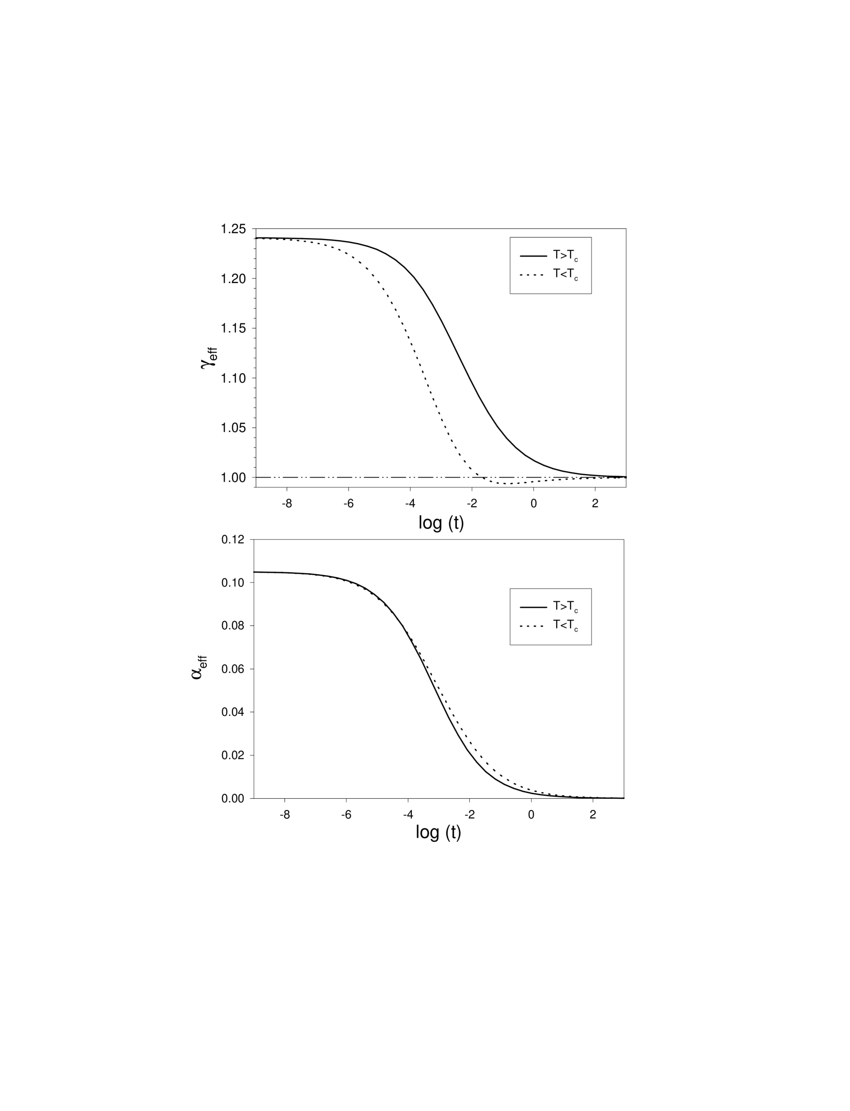
In the present work, the fitting procedure of step 2 of section II A is performed in the entire range of values of . Consequently the entire classical-to-critical crossover specific to the field theoretical framework is completely accounted for by our final functions [see Eqs. (8,9) and tables I–IV]. This is illustrated, for the Ising model (), by fig. (1) which displays the evolution of two effective exponents and , which are defined as for example [see Eqs. (II A)]:
| (7) |
Fig. (1) shows the effective exponents (calculated from the crossover functions of tables I and II) which interpolate between critical and classical (mean field) values following a form of crossover dictated by the framework of field theory. Indeed the (massless or critical, i.e., for ) scalar field theory in three dimensions is defined on a special trajectory of the renormalization group (a renormalized trajectory [26] [RT]) which takes its origin at the Gaussian fixed point (characterized by classical values of the “critical” exponents) and joins the Wilson-Fisher fixed point (where the critical exponents take on their critical values according to the universality class considered). Of course, the crossover so induced is not universal, it is specific of the framework used. In fact, strictly speaking, only the extreme asymptotic moving away from the Wilson-Fisher fixed point induced by small non-zero values of is universal (critical exponents and critical amplitude combinations), even the first-correction amplitude (defined in the close vicinity of the fixed point when is not very small) is not universal. For example, in the present work, a specific definite sign of the first correction amplitude is imposed due to the RT chosen, however in actual systems that kind of correction may well be of the opposite sign and even absent [38]. Fortunately, nonuniversal does not mean necessarily absent in actual critical behaviors. It may well occur that actual systems (or models) display, more or less partially, the kind of crossover calculated from field theory [16, 18, 19, 24, 29, 31]. See section III for a practical use of the crossover functions.
Let us now give some technical informations on the fitting procedure of step 2 of section II A that must be applied two times for each quantity considered because of the two error bounds “” and “” (see sections II A and II B 2 for the meaning of these bounds).
In order to analytically reproduce the functions calculated point by point, we use the following general form [5]:
| (8) |
in which is the maximum number of factors (in a preliminary work [5] we had , in the present work can be as large as ), and with:
| (9) |
in which is the correction exponent. We have adjusted each of the parameters , , , , , and so as to fit the discretized evolutions of the quantities considered (, , , ) as continuous functions of the temperature-like variable in the range . Of course, there are some external constraints on the values of these parameters which facilitate their adjustment:
-
1.
The exponents and must take on values already known from the resummation of the corresponding elementary series.
-
2.
The amplitude is easily determined with few points corresponding to very small values of .
-
3.
To make it easy to get a close reproduction of the crossover towards the classical behavior when , there are constraints:
-
on , so that we have (see, for example, Eqs. (A9, A10) of S. Caracciolo et al. [21]):
(10) this leads to:
(11) -
on one of the couple ’s by imposing that a known classical behavior is reached in the limit then it comes:
(12) (13) with and the classical values of the critical exponents and amplitude respectively. This leads to the constraints for one of the ’s:
(14) (15) with the classical values , , or and or for respectively the susceptibility, the correlation length, the coexistence curve and the specific heat [ is the additive critical part of the specific heat and its classical value; in the inhomogeneous phase (), while in the homogeneous phase ()].
-
With the above prescriptions, we have been able to reproduce the original calculated points with a maximum (local in ) of relative deviation less than (in the worst case and for a limited number of functions especially in the inhomogeneous phase). However, globally (mean value of the local deviations over the entire range of ), the adjustment is much better for all the quantities.
We emphasize that the large number of digits displayed in the tables lays no claim to a better accuracy than in the work of GZ, it is simply required to obtain a careful fit of the crossover functions to the discontinuous points primarily calculated from the available perturbative series.
2 The resummation criteria
In our preceding work [6, 7], the resummation criteria of step 4 of section II A which gave the bounds “” and “” were not chosen so as to closely reproduce the uncertainty of the (at that time up-to-date) estimates of universal asymptotic critical quantities (exponents and amplitude combinations). They simply proceeded from a primary analysis of the convergences of the elementary series [i.e., , , etc ] resulting from the (unique) resummation technique considered. This makes a notable difference because a given function brings several elements into play [see, e.g., Eq. (6)] introducing a possible frustration of the individual resummation criteria. Moreover, when one determines the error bar for an individual quantity, one often rounds it up because several resummation methods may have been considered yielding answers slightly different from each other. Since the various asymptotic critical behaviors of the functions of interest (, etc) result from the combination of a small number of elementary series [39] (namely: , , and a few amplitude functions), the individual criteria were combined in our preceding work [6, 7] so as to provide an envelope of the error accounting automatically for correlations (frustrations) between the error bounds. This has induced some underestimation of the errors when the universal critical exponents or amplitude combinations were (re)-considered from the final expressions of the functions compared to their independent estimates.
The spirit of the present work is different. We have constrained the resummation criteria of the elementary series so as to get as closely as possible the GZ estimates for the universal quantities despite the possible frustrations of the error bounds mentioned above. Thus we have taken into account the extensions up to seven loops of the series for the critical exponents given by Murray and Nickel [28]. For the reasons indicated just above, and also because the error estimates of the amplitude combinations of GZ are deduced from the analysis of the parameter dependence in the equation of state [34] (they have not been obtained from the direct analysis of specific series for the quantities of interest), we have encountered some difficulties in fixing the resummation criteria for some amplitude series (it is likely that GZ have overestimated the error for some quantities). In addition, in doing so and concerning the amplitudes we have introduced an imbalance between the error estimates of the two phases. Indeed our criteria are adjusted so as to get universal ratios (or combinations) of amplitudes which, structurally in the present work, express themselves as series strictly defined in the inhomogeneous phase. On the contrary, the resummation criteria in the homogeneous phase (for only one amplitude function) have been fixed without constraint. Consequently, the resulting error estimates of the correction amplitudes that we presently obtain are larger than in the previous work of refs. [6, 7] and notably in the inhomogeneous phase case; they are presumably overestimated (see below and part III B).
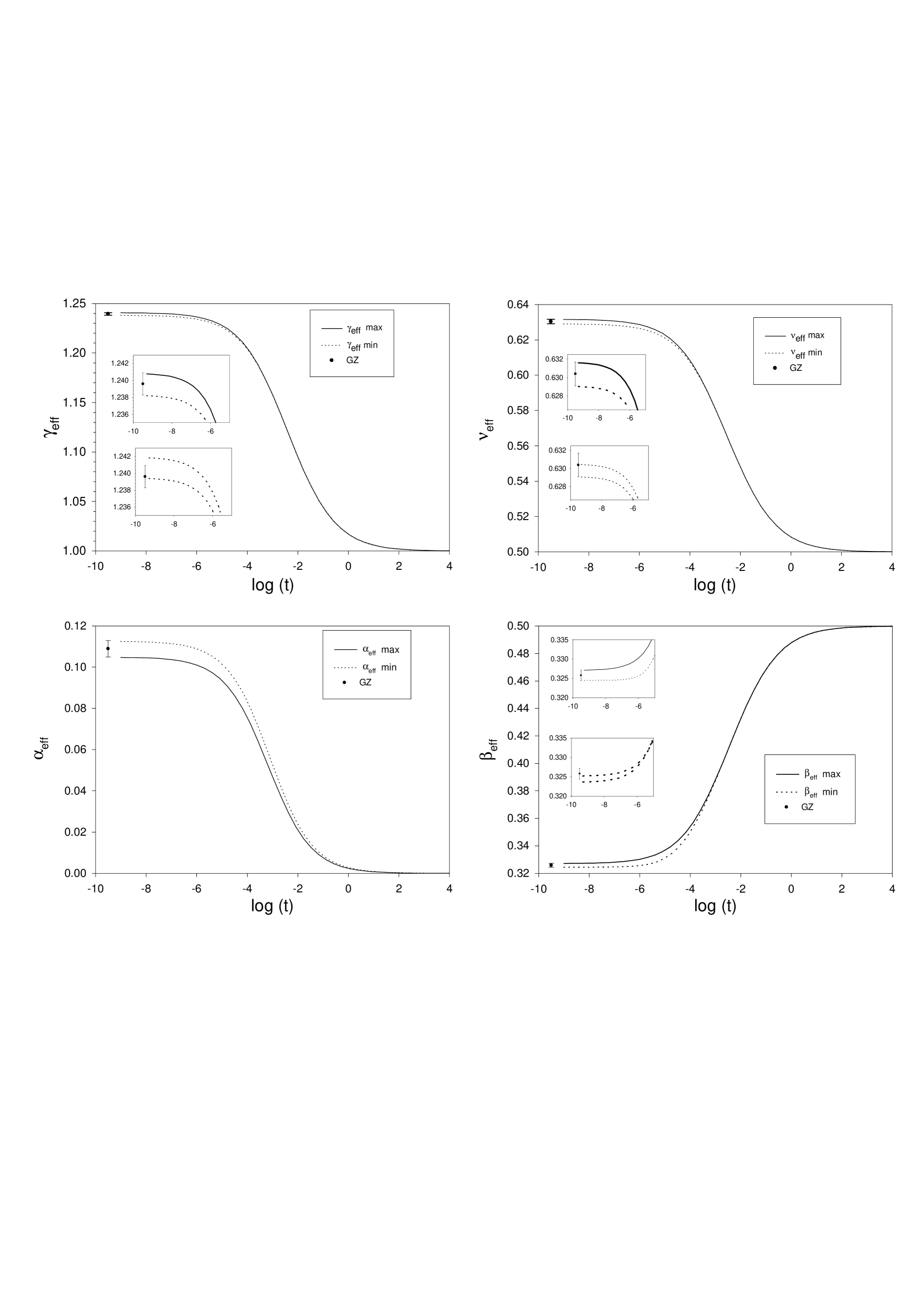
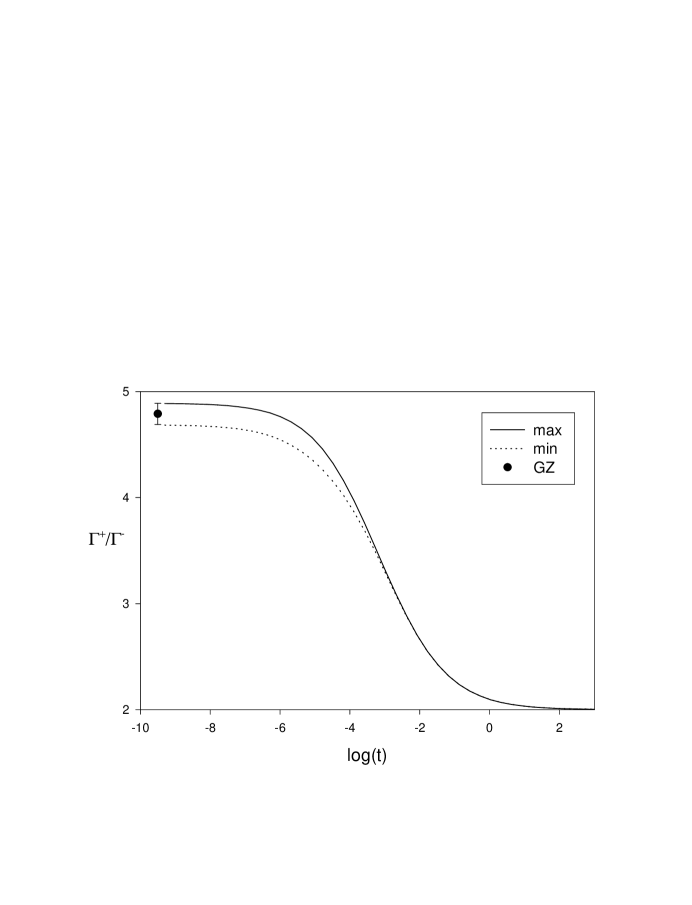
Table V shows our estimates of the critical exponents (resulting from our resummation criteria) compared to the GZ estimates. One may observe some very small differences due to the fact that, in the present work, the scaling relations are automatically satisfied for each bound “” or “” (see step 4 of section II A) while only the central values of the GZ exponent estimates satisfy the scaling relations (the apparent errors for have been determined independently [3]). Table V shows how much the respective estimates meet the scaling relations in both cases. Tables VI and VII display the values of the universal combinations of leading critical amplitudes as they are accounted for by our crossover functions. The degree of agreement with GZ is graphically illustrated by figs (2, 3).
From tables I–IV one may observe that our bounds on the correction exponent differ from GZ. This is due to the correlation of errors mentioned above. Indeed, we have never considered as an independent constituent of the asymptotic critical behavior. Instead it has been (numerically) deduced from the resummation criteria associated with the elementary series and because of the definition with:
| (16) | |||||
| (17) |
The resummation criteria for the elementary series have been chosen so as to yield estimates on the bounds on very close to those of GZ (see table VIII).
Similarly, the present determinations of (and the uncertainties on) the first correction-to-scaling terms displayed in tables IX and X differ from our preceding work [6, 7] essentially because of our systematic account for the up-to-date estimates of the leading amplitude combinations (see tables VI and VII). Notice the likely unrealistic smallness of the correction amplitude in the case “min”. This confirms our probable overestimation of the error on the correction terms (see part III B).
It is worth indicating that the values displayed in tables IX and X are not obtained from the crossover functions of tables I–IV by simply using the expression [see Eq. (8)]:
| (18) |
which would be the right expression if the correction exponent in Eq. (8) was the actual correction exponent instead of the effective exponent of Eq. (9). To get the values displayed in tables IX and X we have made specific fits of the functions of Eq. (8) to the theoretical points with in ranges of values of (as in the preceding work [6, 7]).
III Practical use of the crossover functions
As already said above, the structural form of the classical-to-critical crossover that we produce here is not universal, it is peculiar to the field theoretical framework which corresponds to having performed a limit (the continuum limit) in the renormalization group (RG) theory [40]. The approximation induces the idea that, strictly speaking, the “nonasymptotic” calculations would, in fact, be only valid in the close vicinity of . Hence, we do not expect our functions to reproduce the experimental data in the entire range . However, the width of the domain of agreement between experiments and field theory is not universal: it could actually be reduced (purely and simply) to the strict asymptotic critical region (pure scaling laws) or include exclusively the first correction to scaling, but, fortunately it may sometimes be much larger and could even cover the entire crossover region! It is our aim to allow experimentalists to determine the width of the domain of agreement. Notice that, we do not aim at determining (or providing) all the ingredients needed to describe the variety of classical-to-critical crossovers that may be produced by actual systems, this would be too difficult (due to the infinite variety of nonuniversal contributions). Simply, we think our calculation accurate enough to allow the determination of for any system allowing, in some sense, the determination of subclasses of universality.
As already explained [5, 6, 7], the comparison of the theoretical functions with experimental data involves a very small number of adjustable parameters:
-
1.
Non-universal global factors,
-
2.
The proportionality factor between the temperature like scaling field and (neglecting higher analytical contributions in which may sometimes be non-negligible [10] but are out of the scope of our present aim):
(19) -
3.
Additive regular background terms for the specific heat,
-
4.
Eventually .
For example the comparison with experimental measurements of the susceptibility may be made as follows:
| (20) |
in which represents the experimental data and our function for one [41] of the two bounds “” and “”. One generally expects theoretically that and take on the same values [42] for the two sets of measurements above and below provided that the range of values of is not too large. The fact that must be unchanged is the consequence of the universality of the ratio with as :
| (21) |
in which and are related to our previous definition [Eq. (3)] as follows:
| (22) | |||||
| (23) |
As for the stability of this is because the ratio is universal. The values of the universal amplitude combinations included in our calculated functions are given in tables VI, VII, IX and X.
A Redefinition of the role of
If one introduces literally as in Eq. (19), then the fitted leading critical amplitude involves two adjustable parameters. This is not very suitable. For practical use, we propose to introduce the adjustable parameters as follows [compare with eq (8)]:
| (24) | |||||
| (25) |
in which is no longer involved in the pure scaling part of the critical behavior (). So introduced, is a nonuniversal parameter which exclusively controls the magnitude of the corrections to scaling. Hence we can progressively adjust the theoretical functions to the data starting from the data close to the critical point with and then introducing more and more data with (notice that ) up to the point where consistency is lost.
The domain of where the experimental data and the field theory agree may involve correction-to-scaling terms higher than the first one and this is why it is interesting to have the theoretical expression under the form of a complete classical-to-critical crossover [43].
Consistency test:
If we consider a supplementary set of measurements like the specific heat above and below , then, by virtue of universality, one must obtain again the same value for with a good fit in a range of values of similar to that considered with . For the specific heat, it comes:
| (26) |
in which is an additive non critical (i.e., regular or analytic in ) background and a nonuniversal multiplicative factor which must be the same in the two phases.
Let us emphasize that the field theoretical form obtained for involves a specific critical additive background term which reproduces the famous “classical jump” of the specific heat [see fig (4)]. Of course, the magnitude of this jump is not universal but in the case where an actual system would reproduce the entire classical-to-critical crossover of field theory, then it should also exhibit this jump (up to the global additive background analytic in ).
If, in addition to and , we also possess coexistence curve data, we would have a stronger constraint since then no other adjustable parameter would be required to fit those new data. Indeed in the relation:
| (27) |
everything is fixed since is related to and due to the universal amplitude combination [44] and must have the same value whatever the quantity considered.
If we had simultaneously also access to experimental measurements of the correlation length , then the constraint would be even stronger since again the theory must agree with the data without new adjustable parameter.
B Account for the error bounds
We have accounted for the error estimates by providing two sets (“max” and “min”) of functions. In general the accuracy of the experimental measurements are much smaller than in the present theoretical calculation so that it is not very important to make a difference between the two sets of functions. One or the other choice would provide essentially the same quality of the adjustment in the fitting procedure.
Sometimes accounting for the difference between the bounds “max” and “min” may have some importance so that neither one or the other agrees with the measurements but a mixing of the two would. In such a case we propose to introduce the mixing via the introduction of a supplementary adjustable parameter .
Let us define a new theoretical function as follows
| (28) |
which, regarding the definition of the effective exponents corresponds to the linear weighting:
| (29) |
then the introduction of the other adjustable parameters, such as for example, within is unchanged compare to the description given above.
As said in part II B 2 it is likely that the close account of the GZ estimates has led us to overestimate the uncertainty on the correction terms so that it seems to us useful to provide also the reader with functions reproducing the complete classical-to-critical crossover according to the resummation criteria of the previous (but corrected, see [33]) work of refs [6, 7] although (or rather because), this time, the error are underestimated. This is why we provide two additional text-files of Fortran code [45] corresponding to the former resummation criteria applied to the corrected series (without the seventh order of ref. [28]).
Acknowledgements
We thank Prof. M. Barmatz for interesting correspondence while the present work was in progress.
REFERENCES
- [1] A. Pelissetto and E. Vicari, “Critical phenomena and renormalization-group theory”, cond-mat/0012164 (2000)
- [2] J. Zinn-Justin, in “Euclidean Field Theory and Critical Phenomena”, “Third edition” (Oxford University Press, 1996).
- [3] R. Guida and J. Zinn-Justin, J. Phys. A31, 8103 (1998).
- [4] J. F. Nicoll and J. K. Bhattacharjee, Phys. Rev. B23, 389 (1981). J. F. Nicoll and P. C. Albright, Phys. Rev. B31, 4576 (1985). V. Dohm, Lecture Notes in Physics Vol. 216, p. 263, Ed. by L. Garrido (Springer-Verlag, Pub., 1985). M. A. Anisimov, S. B. Kiselev, J. V. Sengers and S. Tang, Physica A188, 487 (1992).
- [5] C. Bagnuls and C. Bervillier J. Physique Lett. 45, L95 (1984).
- [6] C. Bagnuls and C. Bervillier, Phys. Rev. B32, 7209 (1985).
- [7] C. Bagnuls, C. Bervillier, D. I. Meiron and B. G. Nickel, Phys. Rev. B35, 3585 (1987).
- [8] M. E. Fisher, Rev. Mod. Phys. 46, 597 (1974).
- [9] A. Parola and L. Reatto, Adv. in Phys. 44, 211 (1995).
- [10] M. A. Anisimov and J. V. Sengers, in “Supercritical Fluids - Fundamentals and Applications”, Ed. by E. Kiran, P. G. Debenedetti and C. J. Peters (Kluwer Acad. Pub., 2000).
- [11] K. Binder and E. Luijten, Phys. Rep. 344, 179 (2001).
- [12] M. Corti and V. Degiorgio, Phys. Rev. Lett. 45, 1045 (1980). M. Corti, V. Degiorgio and M. Zulauf, Phys. Rev. Lett. 48, 1617 (1982).
- [13] K. S. Pitzer, Acc. Chem. Res. 23, 333 (1990). H. Weingärtner and W. Schröer, Adv. in Chem. Phys. Vol. 116, p. 1, Ed. by I. Prigogine and S. A. Rice (J. Wiley and Sons, Inc., N.-Y. London, 2001).
- [14] K. Binder, Adv. in Polymer Sci. 112, 181 (1994).
- [15] M. E. Fisher, Phys. Rev. Lett. 57, 1911 (1986); J. Stat. Phys. 75, 1 (1994); J. Phys. C8, 9103 (1996). C. Bagnuls and C. Bervillier, Phys. Rev. Lett. 58, 435 (1987).
- [16] C. Bagnuls and C. Bervillier, Cond. Matt. Phys. 3, 559 (2000).
- [17] E. Luijten, H. W. J. Blöte and K. Binder, Phys. Rev. Lett. 79, 561 (1997); Phys. Rev. E56, 6540 (1997).
- [18] A. Pelissetto, P. Rossi and E. Vicari, Phys. Rev. E58, 7146 (1998).
- [19] S. Caracciolo, M. S. Causo, A. Pelissetto, P. Rossi and E. Vicari, Nucl. Phys. B (Proc. Suppl.) 73, 757 (1999).
- [20] E. Luijten and K. Binder, Phys. Rev. E58, R4060 (1998).
- [21] S. Caracciolo, M. S. Causo, A. Pelissetto, P. Rossi and E. Vicari, Phys. Rev. E64, 046130 (2001).
- [22] K. Binder and E. Luijten, Comp. Phys. Comm. 127, 126 (2000).
- [23] M. A. Anisimov, A. A. Povodyrev, V. D. Kulikov and J. V. Sengers, Phys. Rev. Lett. 75, 3146 (1995); Phys. Rev. Lett. 76, 4095 (1996). C. Bagnuls and C. Bervillier, Phys. Rev. Lett. 76, 4094 (1996). K. Binder, E. Luijten, M. Müller, N. B. Wilding and H. W. J. Blöte, Physica A281, 112 (2000).
- [24] A. Pelissetto, P. Rossi and E. Vicari, Nucl. Phys. B554, 552 (1999).
- [25] The present calculations differ from [18, 24] in that: 1) our treatment is more accurate, 2) the specific heat is considered in the two phases, 3) three values of are treated.
- [26] K. G. Wilson and J. Kogut, Phys. Rep. 12C, 77 (1974). See also: C. Bagnuls and C. Bervillier, J. Phys. Stud. 1, 366 (1997).
- [27] C. Bagnuls and C. Bervillier, Phys. Rep. 348, 91 (2001).
- [28] D. B. Murray and B. G. Nickel, “Revised estimates for critical exponents for the continuum -vector model in dimensions”, unpublished (1991). See also appendix of GZ.
- [29] E. Luijten, H. W. J. Blöte and K. Binder, Phys. Rev. E54, 4626 (1996).
- [30] M. A. Anisimov, E. Luijten, V. A. Agayan, J. V. Sengers and K. Binder, Phys. Lett. A264, 63 (1999).
- [31] E. Luijten and K. Binder, Europhys. Lett. 47, 311 (1999).
- [32] F. J. Halfkann and V. Dohm, Z. Phys. B89, 79 (1992).
- [33] C. Bagnuls, C. Bervillier, D. I. Meiron and B. G. Nickel, “Addendum-erratum to: “Nonasymptotic critical behavior from field theory at . II. The ordered-phase case” Phys. Rev. B35, 3585 (1987).”, hep-th/0006187.
- [34] R. Guida and J. Zinn-Justin, Nucl. Phys. B489, 626 (1997).
- [35] C. Bagnuls and C. Bervillier, in “Fluctuating Paths and Fields”, p. 401, Ed. by W. Janke, A. Pelster, H.-J. Schmidt, M. Bachmann (World Scientific, Singapore, 2001).
- [36] C. Bervillier and C. Godrèche, Phys. Rev. B21, 5427 (1980).
- [37] B. G. Nickel, D. I. Meiron and G. A. Baker, Jr, “Compilation of 2-pt and 4-pt graphs for continuous spin models”, Guelph University preprint, unpublished (1977). May be obtained via the web site http://www.physik.fu-berlin.de/~kleinert/kleiner_reb8/programs/programs.html.
- [38] J. H. Chen, M. E. Fisher and B. G. Nickel, Phys. Rev. Lett. 48, 630 (1982). C. Bagnuls and C. Bervillier, Phys. Rev. B41, 402 (1990); Phys. Lett. A195, 163 (1994). M. Hasenbusch, J. Phys. A34, 8221 (2001). M. Campostrini, M. Hasenbusch, A. Pelissetto, P. Rossi and E. Vicari, Int. J. Mod. Phys. Vol. A16, 2009 (2001). For negative corrections see also: A. Liu and M. E. Fisher, J. Stat. Phys. 58, 431 (1990). L. Schäfer, Phys. Rev. E50, 3517 (1994). A. D. Sokal, Europhys. Lett. 27, 661 (1994).
- [39] That is precisely how universal combinations of amplitudes and scaling relations between exponents occur in the field theoretical framework.
- [40] Only one family of corrections to scaling (controlled by the unique exponent ) is accounted for.
- [41] Or a combination of the two bounds see section III B.
- [42] Generally speaking this is true, but may be nil because there exist systems which do not approach the Ising fixed point along the RG trajectory which links the Gaussian and Ising fixed points. For example some models may have correction-to-scaling terms strictly different from those accounted for by field theory. Also some may have “negative” correction-to-scaling terms. See [38].
- [43] The comparison is made easier than with functions having a limited range of applicability.
- [44] A. Aharony and P. C. Hohenberg, Phys. Rev. B13, 3081 (1976). C. Bervillier, Phys. Rev. B14, 4964 (1976).
- [45] See EPAPS Document No. xxxxxxxxx. Two sets of two files each are provided: first, utdfunctions1.txt and utdfunctionsN.txt which contain the fortran code for the up-to-date crossover functions of respectively tables I and II (Ising like systems in the two phases) in one hand and tables I, III and IV (-vector-like system in the homogeneous phase) in the other hand and second, functions1.txt and functionsN.txt which contain the fortran code for the preceding (corrected, see [33]) work of refs [6, 7]. In each case the file contains its own instructions for use. This document may be retrieve via the EPAPS homepage (http://www.aip.org/pubservs/epaps.html) or from ftp.aip.org in the directory /epaps/. See the EPAPS homepage for more information.

| , homogeneous phase: | ||||||
| — | ||||||
| — | ||||||
| — | — | |||||
| , inhomogeneous phase: | ||||||
| — | — | |||||
| , homogeneous phase: | ||||||
| — | — | |||||
| — | — | |||||
| — | — | |||||
| , homogeneous phase: | ||||||
| — | — | |||||
| critical exponent values | ||||||||||||
|
|
|
|
|
|||||||||
|
|
|
|
— | |||||||||
| 3 |
|
|
|
— | ||||||||
| scaling relations (should be zero) | ||||||||||||
|
|
|
|||||||||||
|
|
— | |||||||||||
| 3 |
|
|||||||||||
|
|
|
|
| 2 | 3 | ||||||||
|---|---|---|---|---|---|---|---|---|---|
|
|
|
|
| 2 | 3 | ||||||||
|---|---|---|---|---|---|---|---|---|---|
|
|
|
|
|
|
|
|
| 1 | 2 | 3 | |||||
|---|---|---|---|---|---|---|---|
| (0.68) |
|
|
|||||
| (8.68) |
|
|
A Computer Program in Fortran
for the Ising model in the two phases
(up-to-date criteria)
       program utdFTcross1
c************************************************
c                   up-to-date                  *
c Crossover functions up to seven loop orders   *
c from Murray-Nickel (1991) and                 *
c accounting for the recent analysis by Guida   *
c and Zinn-Justin [J Phys A31, 8103 (1998)]     *
c************************************************
c For Ising-like systems (n=1) above & below Tc *
c************************************************
c see the companion paper:                      *
C "Classical-to-critical crossovers from field  *
c theory" by C. Bagnuls and C. Bervillier       *
c************************************************
c The important subroutine is
c fns(res,iphase,ibound,ifn,tau,theta,ikont)
c res is the return value of the subroutine
c iphase controls the phase:
c       iphase=1 corresponds to T>Tc
c       iphase=2 corresponds to T<Tc
c ifn controls the type of function chosen:
c       ifn=1 gives the inverse correlation length for T>Tc if iphase=1
c otherwise (iphase=2) it gives the coexistence curve
c       ifn=2 gives the inverse susceptibility
c       ifn=3 gives the specific heat
c ibound controls the accuracy of the theoretical calculation:
c       ibound=1 corresponds to "max"
c       ibound=2 corresponds to "min"
c tau is |T-Tc|/Tc
c theta is the adjustable parameter which relates the scaling field t to tau:
c     (in principle t=theta*tau but for practical use we have separated the asymptotic
c      pure scaling from the correction-to-scaling contributions, see the companion paper,
c      for theta=1 one recovers the pure theoretical
c      functions of the scaling field t)
c ikont is an integer which allows to choose the nature of res
c      if ikont=0 then res gives the functions as indicated above
c      if ikont=1 then res corresponds to the effective exponent associated to the function
c          chosen according to the criteria described above.
c All the functions are for Ising-like model (n=1)
C********************************
      implicit double precision (a-h,o-z)
C*************************************************************
C Evolution of the functions and of the effective exponents  *
C  in terms of the pure scaling field t                      *
C  (i.e., theta=1)                                           *
C*************************************************************
C
C***
C Selection of the function
C***
      iphase=2    ! controls the phase: 1=T>Tc, 2=T<Tc
      ibound=1    ! controls the accuracy bound : 1=max, 2=min
      ifn=3       ! controls the fn: 1=xi, 2=chi, 3=c; for T<Tc, 1=coex curve
C***
C End of selection
C***
C***
C Files for saving the results
C***
      open(29,FILE=’expeff.dat’)
      open(30,FILE=’Funct.dat’)
      theta=1                    ! gives the theoretical evolution in terms of the scaling field t
      t=1.d-9
      do 30 i=1,45
      call fns(f3,iphase,ibound,ifn,t,theta,0)   !Call of the function with ikont=0
      write(30,666) t,f3
      call fns(exp2,iphase,ibound,ifn,t,theta,1)   ! Call of the effective exponent with ikont=1
      print *, t,f3,exp2
      alogt=dlog10(t)
      write(29,666) alogt,exp2     ! Ready for a Log-Lin plot
      t=t*2
30    continue
      close(29)
      close(30)
      stop
666   format(2(G13.6,1x))
      end
C***
C Theoretical functions for n=1
C***
      SUBROUTINE fns(res,i,j,k,t,theta,ikont)
c*************************************************
c if ikont=0: res gives the function
c if ikont=1: res gives the effective exponent
c Table f contains the values of the functions’ parameters.
c At the end of each set a comment allows to distinguish the
c kind of function concerned.
c For each set, the first value is the critical exponent value
c  (or minus this value for the specific heat), the second value
c  is the inverse of the critical amplitude for xi and chi, the
c  critical amplitude for aim and c, the third value is the critical
c  background which is non zero only for c.
c The two values of the subcritical exponent delta corresponding to the two
c bounds "max" and "min" are contained in the table del
c*************************************************
      implicit double precision (a-h,o-z)
      dimension del(2),x(5),y(5)
      dimension f(15,3,2,2)
      data del/0.49862,0.50516/
      data F/0.631678,2.150817,0.,32.24878,32.20434,11.02452,
     #-0.5247187,10.41513,0.3775152,2.315848,-1.307939D-02,
     #39.95028,-1.030731D-01,0.,0.,                                       !ximax  T>Tc (corr length)
     #1.2408875,3.75927,0.,34.05096,34.00404,23.27915,-0.31016527,
     #1.257832,-8.204163D-03,8.313963,-0.1634056,0.,0.,0.,0.,             !chimax  T>Tc (suscept)
     #-.1049675,1.871810,-4.048544,30.37745,30.33559,33.31814,3.476590,
     #9.400643,-8.344217D-03,33.06508,-3.258311,0.,0.,0.,0.,              !cmax  T>Tc (specif heat)
     #0.6290975,2.091612,0.,17.48596,17.57665,10.48005,-0.1283214,
     #28.75634,-9.269701D-02,2.014284,-6.897436D-03,53.07716,
     #-3.027917D-02,0.,0.,                                                !ximin  T>Tc (corr length)
     #1.23830,3.660588,0.,13.38814,13.45758,2.853295,-2.547260D-02,
     #11.51061,-0.2766008,30.25994,-0.1745266,0.,0.,0.,0.,                !chimin  T>Tc (suscept)
     #-.11271,1.580112,-3.548035,33.65919,33.83377,31.94041,
     #0.2200185,7.017899,-9.616869D-03,0.2462918,-7.002609D-05,76.39366,
     #1.508835D-02,0.,0.,                                                 !cmin  T>Tc (specif heat)
     #0.32707350,0.93804691,0.,35.738988,35.689736,
     #303.21696,-0.17687565D-02,9.3779630,0.17204103,1.3921229,
     #0.60877711D-02,30.597947,0.17144092,6.5064180,-0.19479626D-02,      !aimax  T<Tc (coex curve)
     #1.2408875,18.386609,0.,2.3395295,2.3363054,76.549557,-3.4865628,
     #59.838911,-16.395572,3.6904512,0.47894058D-01,63.029796,
     #19.215714,9.3807398,0.13675156,                                     !chimax  T<Tc (suscept)
     #-0.10496750,3.3664988,-4.0481532,1.6036462,1.6014362,
     #79.538017,0.78643478D-01,0.40631542D-01,0.91522424D-04,16.574905,
     #-0.28063252,14.361662,0.13070258,19.477188,0.28112994,              !cmax  T<Tc (specif heat)
     #0.32449540,0.93700952,0.,11.312578,11.371253,
     #241.51662,-0.57056933D-01,13.371447,0.20926322,248.39869,
     #-0.77226529D-02,82.917148,0.15795660,4.7939978,0.48568967D-01,      !aimin  T<Tc (coex curve)
     #1.2383000,17.160196,0.,231.57911,232.78025,23.010983,
     #0.88915951,61.975912,4.0096724,316.29079,-0.15361387,
     #50.582996,-5.2595105,2.5909921,0.37692433D-01,                      !chimin  T<Tc (suscept)
     #-0.11271000,3.0489086,-3.5480350,4.7885026,4.8133395,
     #123.82899,-0.26171236,0.42099375,-0.36312569D-02,10.791900,
     #0.72072941D-01,86.921949,0.41499782,0.57982484,0.36928566D-02/      !cmin  T<Tc (specif heat)
C*********
C  definitions of constants
C*********
      d=del(j)    ! correction exponent
      e=F(1,k,j,i) ! asymptotic exponent
      z=f(2,k,j,i)  ! asymptotic amplitude
      x6=f(3,k,j,i) ! additive critical background
      s1=f(4,k,j,i)
      s2=f(5,k,j,i)
      kmax=0
      do 1 ii=1,5
      x(ii)=f(2*ii+4,k,j,i)    ! definitions of the Xi’s and Yi’s
      if(x(ii).eq.0.) go to 2
      y(ii)=f(2*ii+5,k,j,i)
1     kmax=kmax+1
2     continue
      if(ikont.eq.0) then    ! calculation of the function
      res=Z*t**e
      if(theta.eq.0.) then   ! If theta=0
      res=res+x6             ! there is no correction-to-scaling
      return                 ! only the pure scaling form
      end if                 ! survives
      tt=theta*t
      D=D-1+(S1*dsqrt(tt)+1)/(S2*dsqrt(tt)+1)
      trr=(tt)**D
      do 3 kk=1,kmax
3     res=res*(1+X(kk)*trr)**Y(kk)
      res=res+X6
      return
      end if
      if(ikont.eq.1) then    ! calculation of the effective exponent
      if(theta.eq.0) then   ! If theta=0
      res=e                 ! then
      if(k.eq.3) res=-res   ! the effective exponent
      return                ! reduces to the constant
      end if                ! critical exponent
      tt=theta*t
      D=D-1+(S1*dsqrt(tt)+1)/(S2*dsqrt(tt)+1)
      trr=(tt)**D
      Dp=(S1-S2)/(2*dsqrt(tt)*(S2*dsqrt(tt)+1)**2)
      res=0.
      do 4 kk=1,kmax
4     res=res+X(kk)*Y(kk)/(1+X(kk)*trr)
      res=res*(Dp*tt*DLOG(tt)+D)*trr
      res=res+e
      if(k.eq.3) res=-res     ! the exponent changes sign for c
      return
      end if
      print *, "Error, ikont is ",ikont, ", but must be 0 or 1."
      stop
      end
B Computer Program in Fortran
for the -vector model () in the homogeneous phase
(up-to-date criteria)
      program utdFTcrossN
c************************************************
c                   up-to-date                  *
c Crossover functions up to seven loop orders   *
c from Murray-Nickel (1991) and                 *
c accounting for the recent analysis by Guida   *
c and Zinn-Justin [J Phys A31, 8103 (1998)]     *
c************************************************
c For N-vector-like systems (n=1, 2, 3)         *
c in the homogeneous phase only                 *
c************************************************
c see the companion paper:                      *
C "Classical-to-critical crossovers from field  *
c theory" by C. Bagnuls and C. Bervillier       *
c************************************************
c The important subroutine is
c fns(res,iN,ibound,ifn,tau,theta,ikont)
c res is the return value of the subroutine
c iN controls the value of n:
c       iN=1 corresponds to n=1
c       iN=2 corresponds to n=2
c       iN=3 corresponds to n=3
c ifn controls the type of function chosen:
c       ifn=1 gives the inverse correlation length
c       ifn=2 gives the inverse susceptibility
c       ifn=3 gives the specific heat
c ibound controls the accuracy of the theoretical calculation:
c       ibound=1 corresponds to "max"
c       ibound=2 corresponds to "min"
c tau is |T-Tc|/Tc
c theta is the adjustable parameter which relates the scaling field t to tau:
c     (in principle t=theta*tau but for practical use we have separated the asymptotic
c      pure scaling from the correction-to-scaling contributions, see the companion paper,
c      for theta=1 one recovers the pure theoretical
c      functions of the scaling field t)
c ikont is an integer which allows to choose the nature of res
c      if ikont=0 then res gives the functions as indicated above
c      if ikont=1 then res corresponds to the effective exponent associated to the function
c          chosen according to the criteria described above.
C********************************
      implicit double precision (a-h,o-z)
C*************************************************************
C Evolution of the functions and of the effective exponents  *
C  in terms of the pure scaling field t                      *
C  (i.e., theta=1)                                           *
C*************************************************************
C
C***
C Selection of the function
C***
      iN=2        ! controls the value of n: 1, 2, or 3
      ibound=1    ! controls the accuracy bound : 1=max, 2=min
      ifn=3       ! controls the fn: 1=xi, 2=chi, 3=c
C***
C End of selection
C***
C***
C Files for saving the results
C***
      open(29,FILE=’expeff.dat’)
      open(30,FILE=’Funct.dat’)
      theta=1                    ! gives the theoretical evolution in terms of the scaling field t
      t=1.d-9
      do 30 i=1,45
      call fns(f3,iN,ibound,ifn,t,theta,0)   !Call of the function with ikont=0
      write(30,666) t,f3
      call fns(exp2,iN,ibound,ifn,t,theta,1)   ! Call of the effective exponent with ikont=1
      print *, t,f3,exp2
      alogt=dlog10(t)
      write(29,666) alogt,exp2     ! Ready for a Log-Lin plot
      t=t*2
30    continue
      close(29)
      close(30)
      stop
666   format(2(G13.6,1x))
      end
C***
C Theoretical functions for n-vector-like systems
C***
      SUBROUTINE fns(res,i,j,k,t,theta,ikont)
c*************************************************
c if ikont=0: res gives the function
c if ikont=1: res gives the effective exponent
c Table f contains the values of the functions’ parameters.
c At the end of each set a comment allows to distinguish the
c kind of function concerned.
c For each set, the first value is the critical exponent value
c  (or minus this value for the specific heat), the second value
c  is the inverse of the critical amplitude for xi and chi, the
c  critical amplitude for c, the third value is the critical
c  background which is non zero only for c.
c The six values of the subcritical exponent delta corresponding to the two
c bounds "max" and "min" for each value of n are contained in the table del
c*************************************************
      implicit double precision (a-h,o-z)
      dimension del(2,3),x(5),y(5)
      dimension f(15,3,2,3)
      data del/0.49862,0.50516,0.52551,0.52986,0.55227,0.55702/
      data F/0.631678,2.150817,0.,32.24878,32.20434,11.02452,
     #-0.5247187,10.41513,0.3775152,2.315848,-1.307939D-02,
     #39.95028,-1.030731D-01,0.,0.,                                       !ximax n=1 (corr length)
     #1.2408875,3.75927,0.,34.05096,34.00404,23.27915,-0.31016527,
     #1.257832,-8.204163D-03,8.313963,-0.1634056,0.,0.,0.,0.,             !chimax n=1 (suscept)
     #-.1049675,1.871810,-4.048544,30.37745,30.33559,33.31814,3.476590,
     #9.400643,-8.344217D-03,33.06508,-3.258311,0.,0.,0.,0.,              !cmax n=1 (specif heat)
     #0.6290975,2.091612,0.,17.48596,17.57665,10.48005,-0.1283214,
     #28.75634,-9.269701D-02,2.014284,-6.897436D-03,53.07716,
     #-3.027917D-02,0.,0.,                                                !ximin  n=1 (corr length)
     #1.23830,3.660588,0.,13.38814,13.45758,2.853295,-2.547260D-02,
     #11.51061,-0.2766008,30.25994,-0.1745266,0.,0.,0.,0.,                !chimin  n=1 (suscept)
     #-.11271,1.580112,-3.548035,33.65919,33.83377,31.94041,
     #0.2200185,7.017899,-9.616869D-03,0.2462918,-7.002609D-05,76.39366,
     #1.508835D-02,0.,0.,                                                 !cmin  n=1 (specif heat)
     #0.67181082,2.6289918,0.,15.963748,16.381644,
     #28.529734,-0.90963764D-01,9.1112497,-0.22311836,0.11326011,
     #0.38347877D-03,72.907613,-0.50166740D-01,10.299474,0.20243740D-01,  !ximax n=2 (corr length)
     #1.3188985,5.5612909,0.,96.831346,99.366178,
     #16.310867,-0.57358194,3.6615694,-0.56950360D-01,0.32669257,
     #-0.48535318D-03,430.16727,-0.67793463D-02,0.,0.,                    !chimax n=2 (suscept)
     #0.15440000D-01,-55.881907,50.158572,4.0480920,4.1540622,
     #1.1911602,0.55704053D-01,1.2675164,-0.58499557D-01,27.562173,
     #-0.77243929D-02,46.806723,-0.20360103D-01,0.,0.,                    !cmax n=2 (specif heat)
     #0.66878932,2.5496125,0.,33.474847,34.505171,
     #111.52736,-0.28491431D-01,13.427180,-15.783043,24.100833,
     #0.18612028D-02,13.360107,15.603262,7.3960558,-0.13116817,           !ximin  n=2 (corr length)
     #1.3148952,5.3464216,0.,60.160224,62.011900,
     #11.716728,-0.41213479D-01,15.104245,-0.53630510,3.1051883,
     #-0.38536260D-01,239.95179,-0.13735564D-01,0.,0.,                    !chimin  n=2 (suscept)
     #0.63700000D-02,-121.13056,115.95104,28.884078,29.773102,
     #37.837491,3.5434706,59.951524,-0.17677012D-01,1.3847300,
     #0.22769060D-03,37.714984,-3.5387612,0.,0.,                          !cmin  n=2 (specif heat)
     #0.71090629,3.1722403,0.,31.477107,33.213159,
     #394.95293,-0.52545625D-02,0.15078920,0.28641031D-02,11.387266,
     #-0.35982658,78.089588,-0.56692560D-01,0.19582193,-0.29029786D-02,   !ximax n=3 (corr length)
     #1.3946000,7.9856105,0.,72.301387,76.289014,
     #13.735280,-0.75390860,1.3616777,0.46960131,1.3862969,
     #-0.49056204,437.65747,-0.14330672D-01,0.,0.,                        !chimax n=3 (suscept)
     #0.13272000,-20.228436,8.2684338,17.216858,18.166416,
     #389.17897,-0.30498190D-02,0.47607464D-01,0.32528813D-03,12.991689,
     #-0.16565010,65.185231,-0.10948246,1.7080277,0.12417093D-01,         !cmax n=3 (specif heat)
     #0.70381062,2.9632572,0.,78.590543,83.342746,
     #10.931307,16.025379,3.2123716,-0.11355993,505.59521,
     #-0.69793726D-02,11.021201,-16.378555,2.8188361,0.66094313D-01,      !ximin  n=3 (corr length)
     #1.3845100,7.2687650,0.,52.048362,55.195616,
     #0.15890396,0.11525134D-02,11.028433,-0.47495792D-01,12.528570,
     #-0.69601028,312.81912,-0.18816147D-01,0.97748668,-0.78502947D-02,   !chimin  n=3 (suscept)
     #0.11143582,-18.976690,9.1558605,96640.818,102484.48,
     #52.385639,0.19945718,1179.5468,0.13062104D-02,22.441166,
     #-0.13439992,36.340773,-0.35127870,11.698778,0.62043595D-01/         !cmin  n=3 (suscept)
C*********
C  definitions of constants
C*********
      if(i.gt.3.or.i.lt.1) then
      print *, "Error, n= ",i, "is not available. Sorry. (0<n<4)"
      stop
      end if
      d=del(j,i)    ! correction exponent
      e=F(1,k,j,i) ! asymptotic exponent
      z=f(2,k,j,i)  ! asymptotic amplitude
      x6=f(3,k,j,i) ! additive critical background
      s1=f(4,k,j,i)
      s2=f(5,k,j,i)
      kmax=0
      do 1 ii=1,5
      x(ii)=f(2*ii+4,k,j,i)    ! definitions of the Xi’s and Yi’s
      if(x(ii).eq.0.) go to 2
      y(ii)=f(2*ii+5,k,j,i)
1     kmax=kmax+1
2     continue
      if(ikont.eq.0) then    ! calculation of the function
      res=Z*t**e
      if(theta.eq.0.) then   ! If theta=0
      res=res+x6             ! there is no correction-to-scaling
      return                 ! only the pure scaling form
      end if                 ! survives
      tt=theta*t
      D=D-1+(S1*dsqrt(tt)+1)/(S2*dsqrt(tt)+1)
      trr=(tt)**D
      do 3 kk=1,kmax
3     res=res*(1+X(kk)*trr)**Y(kk)
      res=res+X6
      return
      end if
      if(ikont.eq.1) then    ! calculation of the effective exponent
      if(theta.eq.0) then   ! If theta=0
      res=e                 ! then
      if(k.eq.3) res=-res  ! the effective exponent
      return                ! reduces to the constant
      end if                ! critical exponent
      tt=theta*t
      D=D-1+(S1*dsqrt(tt)+1)/(S2*dsqrt(tt)+1)
      trr=(tt)**D
      Dp=(S1-S2)/(2*dsqrt(tt)*(S2*dsqrt(tt)+1)**2)
      res=0.
      do 4 kk=1,kmax
4     res=res+X(kk)*Y(kk)/(1+X(kk)*trr)
      res=res*(Dp*tt*DLOG(tt)+D)*trr
      res=res+e
      if(k.eq.3) res=-res  ! the exponent changes sign for c
      return
      end if
      print *, "Error, ikont is ",ikont, ", but must be 0 or 1."
      stop
      end
C Computer Program in Fortran
for the Ising model in the two phases
(former criteria, corrected series)
      program FTcross1
c************************************************
c            former corrected                   *
c Crossover functions up to six loop orders     *
c after correction of the errors for the        *
c inhomogeneous phase                           *
c************************************************
c For Ising-like systems (n=1) above & below Tc *
c************************************************
c see the companion paper:                      *
C "Classical-to-critical crossovers from field  *
c theory" by C. Bagnuls and C. Bervillier       *
c************************************************
c The important subroutine is
c fns(res,iphase,ibound,ifn,tau,theta,ikont)
c res is the return value of the subroutine
c iphase controls the phase:
c       iphase=1 corresponds to T>Tc
c       iphase=2 corresponds to T<Tc
c ifn controls the type of function chosen:
c       ifn=1 gives the inverse correlation length for T>Tc if iphase=1
c otherwise (iphase=2) it gives the coexistence curve
c       ifn=2 gives the inverse susceptibility
c       ifn=3 gives the specific heat
c ibound controls the accuracy of the theoretical calculation:
c       ibound=1 corresponds to "max"
c       ibound=2 corresponds to "min"
c tau is |T-Tc|/Tc
c theta is the adjustable parameter which relates the scaling field t to tau:
c     (in principle t=theta*tau but for practical use we have separated the asymptotic
c      pure scaling from the correction-to-scaling contributions, see the companion paper,
c      for theta=1 one recovers the pure theoretical
c      functions of the scaling field t)
c ikont is an integer which allows to choose the nature of res
c      if ikont=0 then res gives the functions as indicated above
c      if ikont=1 then res corresponds to the effective exponent associated to the function
c          chosen according to the criteria described above.
c All the functions are for Ising-like model (n=1)
C********************************
      implicit double precision (a-h,o-z)
C*************************************************************
C Evolution of the functions and of the effective exponents  *
C  in terms of the pure scaling field t                      *
C  (i.e., theta=1)                                           *
C*************************************************************
C
C***
C Selection of the function
C***
      iphase=2    ! controls the phase: 1=T>Tc, 2=T<Tc
      ibound=1    ! controls the accuracy bound : 1=max, 2=min
      ifn=3       ! controls the fn: 1=xi, 2=chi, 3=c; for T<Tc, 1=coex curve
C***
C End of selection
C***
C***
C Files for saving the results
C***
      open(29,FILE=’expeff.dat’)
      open(30,FILE=’Funct.dat’)
      theta=1                    ! gives the theoretical evolution in terms of the scaling field t
      t=1.d-9
      do 30 i=1,45
      call fns(f3,iphase,ibound,ifn,t,theta,0)   !Call of the function with ikont=0
      write(30,666) t,f3
      call fns(exp2,iphase,ibound,ifn,t,theta,1)   ! Call of the effective exponent with ikont=1
      print *, t,f3,exp2
      alogt=dlog10(t)
      write(29,666) alogt,exp2     ! Ready for a Log-Lin plot
      t=t*2
30    continue
      close(29)
      close(30)
      stop
666   format(2(G13.6,1x))
      end
C***
C Theoretical functions for n=1
C***
      SUBROUTINE fns(res,i,j,k,t,theta,ikont)
c*************************************************
c if ikont=0: res gives the function
c if ikont=1: res gives the effective exponent
c Table f contains the values of the functions’ parameters.
c At the end of each set a comment allows to distinguish the
c kind of function concerned.
c For each set, the first value is the critical exponent value
c  (or minus this value for the specific heat), the second value
c  is the inverse of the critical amplitude for xi and chi, the
c  critical amplitude for aim and c, the third value is the critical
c  background which is non zero only for c.
c The two values of the subcritical exponent delta corresponding to the two
c bounds "max" and "min" are contained in the table del
c*************************************************
      implicit double precision (a-h,o-z)
      dimension del(2),x(5),y(5)
      dimension f(15,3,2,2)
      data del/0.49125,0.50031/
      data F/0.630501,2.12411,0.,16.87409,16.72772,23.51302,-0.2154827,
     #0.6009808,-1.955281D-03,5.460931,-4.356399D-02,0.,0.,0.,0.,         !ximax  T>Tc (corr length)
     #1.24194,3.80403,0.,10.7784,10.6849,18.2831,-0.447952,0.211862,
     #-1.12883D-03,2.82005,-3.47989D-02,0.,0.,0.,0.,                      !chimax  T>Tc (suscept)
     #-.108496,1.74928,-3.87997,22077.0,21885.5,8.15287,-8.12340D-03,
     #36.4432,0.223350,395.406,1.76520D-03,0.,0.,0.,0.,                   !cmax  T>Tc (specif heat)
     #0.629121,2.09256,0.,1.793553,1.794109,32.37368,-0.1214804,
     #11.42729,-0.1263489,2.192044,-1.041270D-02,0.,0.,0.,0.,             !ximin  T>Tc (corr length)
     #1.239485,3.706359,0.,1.229767,1.230149,2.198050,-2.015454D-02,
     #24.55992,-0.2546755,10.44460,-0.2041400,0.,0.,0.,0.,                !chimin  T>Tc (suscept)
     #-.112636,1.58819,-3.57607,69.75599,69.77762,11.38361,
     #-1.004983D-01,11.37558,8.030914D-02,33.34772,0.2454611,0.,0.,0.,
     #0.,                                                                 !cmin  T>Tc (specif heat)
     #0.32516,0.9213251,0.,64.93122,64.36800,1.770551,1.028455D-02,
     #46.28114,0.1928966,89.74606,-5.501773D-02,10.80746,0.2015166,0.,
     #0.,                                                                 !aimax  T<Tc (coex curve)
     #1.24194,19.19139,0.,8.662018,8.586883,8.293155,0.2623473,
     #37.19002,-1.070686,71.02634,-2.254137,62.54640,2.578595,
     #0.,0.,                                                              !chimax  T<Tc (suscept)
     #-.108496,3.184180,-3.879732,49.56056,49.13067,4.262502,
     #6.145600D-03,66.44198,0.1076623,20.11234,1.031841D-01,0.,0.,0.,0.,  !cmax  T<Tc (specif heat)
     #0.32357,0.8971946,0.,13.29911,13.30323,131.5962,2.430934D-02,
     #1.304663,4.734644D-03,23.57031,0.1913076,8.270542,0.1325084,0.,0.,  !aimin  T<Tc (coex curve)
     #1.239485,16.78313,0.,360.4357,360.5474,22.85732,0.4525390,
     #204.6138,5.788026D-02,3.581834,6.527502D-02,41.70674,-1.054664,
     #0.,0.,                                                              !chimin  T<Tc (suscept)
     #-0.112636,3.004344,-3.576325,225.67103,225.74101,13.429043,
     #7.624208D-02,183.93336,-29.012144,56.400856,0.16278169,183.93769,
     #28.998392,0.,0./                                                    !cmin  T<Tc (specif heat)
C*********
C  definitions of constants
C*********
      d=del(j)    ! correction exponent
      e=F(1,k,j,i) ! asymptotic exponent
      z=f(2,k,j,i)  ! asymptotic amplitude
      x6=f(3,k,j,i) ! additive critical background
      s1=f(4,k,j,i)
      s2=f(5,k,j,i)
      kmax=0
      do 1 ii=1,5
      x(ii)=f(2*ii+4,k,j,i)    ! definitions of the Xi’s and Yi’s
      if(x(ii).eq.0.) go to 2
      y(ii)=f(2*ii+5,k,j,i)
1     kmax=kmax+1
2     continue
      if(ikont.eq.0) then    ! calculation of the function
      res=Z*t**e
      if(theta.eq.0.) then   ! If theta=0
      res=res+x6             ! there is no correction-to-scaling
      return                 ! only the pure scaling form
      end if                 ! survives
      tt=theta*t
      D=D-1+(S1*dsqrt(tt)+1)/(S2*dsqrt(tt)+1)
      trr=(tt)**D
      do 3 kk=1,kmax
3     res=res*(1+X(kk)*trr)**Y(kk)
      res=res+X6
      return
      end if
      if(ikont.eq.1) then    ! calculation of the effective exponent
      if(theta.eq.0) then   ! If theta=0
      res=e                 ! then
      if(k.eq.3) res=-res   ! the effective exponent
      return                ! reduces to the constant
      end if                ! critical exponent
      tt=theta*t
      D=D-1+(S1*dsqrt(tt)+1)/(S2*dsqrt(tt)+1)
      trr=(tt)**D
      Dp=(S1-S2)/(2*dsqrt(tt)*(S2*dsqrt(tt)+1)**2)
      res=0.
      do 4 kk=1,kmax
4     res=res+X(kk)*Y(kk)/(1+X(kk)*trr)
      res=res*(Dp*tt*DLOG(tt)+D)*trr
      res=res+e
      if(k.eq.3) res=-res     ! the exponent changes sign for c
      return
      end if
      print *, "Error, ikont is ",ikont, ", but must be 0 or 1."
      stop
      end
D Computer Program in Fortran
for the -vector model () in the homogeneous phase
(former criteria)
      program FTcrossN
c************************************************
c            former                             *
c Crossover functions up to six loop orders     *
c************************************************
c For N-vector-like systems (n=1, 2, 3)         *
c in the homogeneous phase only                 *
c************************************************
c see the companion paper:                      *
C "Classical-to-critical crossovers from field  *
c theory" by C. Bagnuls and C. Bervillier       *
c************************************************
c The important subroutine is
c fns(res,iN,ibound,ifn,tau,theta,ikont)
c res is the return value of the subroutine
c iN controls the value of n:
c       iN=1 corresponds to n=1
c       iN=2 corresponds to n=2
c       iN=3 corresponds to n=3
c ifn controls the type of function chosen:
c       ifn=1 gives the inverse correlation length
c       ifn=2 gives the inverse susceptibility
c       ifn=3 gives the specific heat
c ibound controls the accuracy of the theoretical calculation:
c       ibound=1 corresponds to "max"
c       ibound=2 corresponds to "min"
c tau is |T-Tc|/Tc
c theta is the adjustable parameter which relates the scaling field t to tau:
c     (in principle t=theta*tau but for practical use we have separated the asymptotic
c      pure scaling from the correction-to-scaling contributions, see the companion paper,
c      for theta=1 one recovers the pure theoretical
c      functions of the scaling field t)
c ikont is an integer which allows to choose the nature of res
c      if ikont=0 then res gives the functions as indicated above
c      if ikont=1 then res corresponds to the effective exponent associated to the function
c          chosen according to the criteria described above.
C********************************
      implicit double precision (a-h,o-z)
C*************************************************************
C Evolution of the functions and of the effective exponents  *
C  in terms of the pure scaling field t                      *
C  (i.e., theta=1)                                           *
C*************************************************************
C
C***
C Selection of the function
C***
      iN=2        ! controls the value of n: 1, 2, or 3
      ibound=1    ! controls the accuracy bound : 1=max, 2=min
      ifn=3       ! controls the fn: 1=xi, 2=chi, 3=c
C***
C End of selection
C***
C***
C Files for saving the results
C***
      open(29,FILE=’expeff.dat’)
      open(30,FILE=’Funct.dat’)
      theta=1                    ! gives the theoretical evolution in terms of the scaling field t
      t=1.d-9
      do 30 i=1,45
      call fns(f3,iN,ibound,ifn,t,theta,0)   !Call of the function with ikont=0
      write(30,666) t,f3
      call fns(exp2,iN,ibound,ifn,t,theta,1)   ! Call of the effective exponent with ikont=1
      print *, t,f3,exp2
      alogt=dlog10(t)
      write(29,666) alogt,exp2     ! Ready for a Log-Lin plot
      t=t*2
30    continue
      close(29)
      close(30)
      stop
666   format(2(G13.6,1x))
      end
C***
C Theoretical functions for n-vector-like systems
C***
      SUBROUTINE fns(res,i,j,k,t,theta,ikont)
c*************************************************
c if ikont=0: res gives the function
c if ikont=1: res gives the effective exponent
c Table f contains the values of the functions’ parameters.
c At the end of each set a comment allows to distinguish the
c kind of function concerned.
c For each set, the first value is the critical exponent value
c  (or minus this value for the specific heat), the second value
c  is the inverse of the critical amplitude for xi and chi, the
c  critical amplitude for c, the third value is the critical
c  background which is non zero only for c.
c The six values of the subcritical exponent delta corresponding to the two
c bounds "max" and "min" for each value of n are contained in the table del
c*************************************************
      implicit double precision (a-h,o-z)
      dimension del(2,3),x(5),y(5)
      dimension f(15,3,2,3)
      data del/0.49125,0.50031,0.52012,0.52737,0.54975,0.55043/
      data F/0.630501,2.12411,0.,16.87409,16.72772,23.51302,-0.2154827,
     #0.6009808,-1.955281D-03,5.460931,-4.356399D-02,0.,0.,0.,0.,       !ximax T>Tc n=1 (corr length)
     #1.24194,3.80403,0.,10.7784,10.6849,18.2831,-0.447952,0.211862,
     #-1.12883D-03,2.82005,-3.47989D-02,0.,0.,0.,0.,                    !chimax T>Tc n=1 (suscept)
     #-.108496,1.74928,-3.87997,22077.0,21885.5,8.15287,-8.12340D-03,
     #36.4432,0.223350,395.406,1.76520D-03,0.,0.,0.,0.,                 !cmax T>Tc n=1 (specif heat)
     #0.629121,2.09256,0.,1.793553,1.794109,32.37368,-0.1214804,
     #11.42729,-0.1263489,2.192044,-1.041270D-02,0.,0.,0.,0.,           !ximin  T>Tc n=1 (corr length)
     #1.239485,3.706359,0.,1.229767,1.230149,2.198050,-2.015454D-02,
     #24.55992,-0.2546755,10.44460,-0.2041400,0.,0.,0.,0.,              !chimin  T>Tc n=1 (suscept)
     #-.112636,1.58819,-3.57607,69.75599,69.77762,11.38361,
     #-1.004983D-01,11.37558,8.030914D-02,33.34772,0.2454611,0.,0.,0.,
     #0.,                                                               !cmin  T>Tc n=1 (specif heat)
     #0.669848,2.578296,0.,28.84310,29.43534,15.75544,-0.2585115,
     #5.012764,-4.343250D-02,77.73647,-3.775196D-02,0.,0.,0.,0.,        !ximax T>Tc n=2 (corr length)
     #1.31792,5.51529,0.,63.8357,65.1464,16.9739,-0.508216,
     #1.85577,-1.44706D-02,7.33240,-1.03476D-01,247.042,-9.67699D-03,
     #0.,0.,                                                            !chimax T>Tc n=2 (suscept)
     #9.488051D-03,-85.85105,80.36121,457.8256,467.2262,21.93721,
     #-4.630859D-02,11.62941,-9.686347D-03,15.18151,3.701884D-02,
     #0.,0.,0.,0.,                                                      !cmax T>Tc n=2 (specif heat)
     #0.6678685,2.527959,0.,92.02055,94.61002,1.400964,-3.366864D-03,
     #5.520135,-4.367003D-02,395.4183,-4.673720D-03,18.17701,
     #-0.2840264,0.,0.,                                                 !ximin  T>Tc n=2 (corr length)
     #1.314001,5.307447,0.,60.60521,62.31065,15.15227,-0.5613569,
     #2.473990,-2.203622D-02,5.819209,-3.266531D-02,246.3158,
     #-1.194353D-02,0.,0.,                                              !chimin  T>Tc n=2 (suscept)
     #3.603233D-03,-207.0019,201.9794,367.4423,377.7822,17.09462,
     #-12.10980,3.267621,-1.663525D-04,17.08843,12.10276,0.,0.,0.,0.,   !cmin  T>Tc n=2 (specif heat)
     #0.7056167,3.014192,0.,76.15010,80.13691,4.745939,-8.777504D-02,
     #445.7242,-7.186912D-03,8.077017,0.2125871,13.25811,-0.5288586,
     #0.,0.,                                                            !ximax T>Tc n=3 (corr length)
     #1.389161,7.591932,0.,27.84825,29.30624,10.79849,-0.6921719,
     #5.606645D-02,5.519555D-04,316.7178,-8.449968D-03,67.73494,
     #-7.825108D-02,0.,0.,                                              !chimax T>Tc n=3 (suscept)
     #0.1168480,-19.46045,8.971331,69.91117,73.57134,389.0545,
     #-7.759979D-03,15.08428,-1.794460,0.2445648,3.624132D-04,
     #14.03141,1.568162,0.,0.,                                          !cmax T>Tc n=3 (specif heat)
     #0.7038317,2.969913,0.,78.53203,82.70273,12.80904,-0.5435931,
     #5.710801,-0.3817143,463.4073,-6.842927D-03,6.792342,0.5244869,
     #0.,0.,                                                            !ximin  T>Tc n=3 (corr length)
     #1.383616,7.231499,0.,48.19012,50.74942,12.44953,-0.7397974,
     #0.5892605,0.2315015,0.6046381,-0.2390366,260.9201,
     #-1.990006D-02,0.,0.,                                              !chimin  T>Tc n=3 (suscept)
     #0.1114902,-19.09212,9.185812,2.689863,2.832717,40.48173,
     #-0.1850101,1.173960,-0.1448486,1.743464D-02,6.113689D-04,
     #0.8190587,0.1062669,0.,0./                                        !cmin  T>Tc n=3 (suscept)
C*********
C  definitions of constants
C*********
      if(i.gt.3.or.i.lt.1) then
      print *, "Error, n= ",i, "is not available. Sorry. (0<n<4)"
      stop
      end if
      d=del(j,i)    ! correction exponent
      e=F(1,k,j,i) ! asymptotic exponent
      z=f(2,k,j,i)  ! asymptotic amplitude
      x6=f(3,k,j,i) ! additive critical background
      s1=f(4,k,j,i)
      s2=f(5,k,j,i)
      kmax=0
      do 1 ii=1,5
      x(ii)=f(2*ii+4,k,j,i)    ! definitions of the Xi’s and Yi’s
      if(x(ii).eq.0.) go to 2
      y(ii)=f(2*ii+5,k,j,i)
1     kmax=kmax+1
2     continue
      if(ikont.eq.0) then    ! calculation of the function
      res=Z*t**e
      if(theta.eq.0.) then   ! If theta=0
      res=res+x6             ! there is no correction-to-scaling
      return                 ! only the pure scaling form
      end if                 ! survives
      tt=theta*t
      D=D-1+(S1*dsqrt(tt)+1)/(S2*dsqrt(tt)+1)
      trr=(tt)**D
      do 3 kk=1,kmax
3     res=res*(1+X(kk)*trr)**Y(kk)
      res=res+X6
      return
      end if
      if(ikont.eq.1) then    ! calculation of the effective exponent
      if(theta.eq.0) then   ! If theta=0
      res=e                 ! then
      if(k.eq.3) res=-res   ! the effective exponent
      return                ! reduces to the constant
      end if                ! critical exponent
      tt=theta*t
      D=D-1+(S1*dsqrt(tt)+1)/(S2*dsqrt(tt)+1)
      trr=(tt)**D
      Dp=(S1-S2)/(2*dsqrt(tt)*(S2*dsqrt(tt)+1)**2)
      res=0.
      do 4 kk=1,kmax
4     res=res+X(kk)*Y(kk)/(1+X(kk)*trr)
      res=res*(Dp*tt*DLOG(tt)+D)*trr
      res=res+e
      if(k.eq.3) res=-res  ! the exponent changes sign for c
      return
      end if
      print *, "Error, ikont is ",ikont, ", but must be 0 or 1."
      stop
      end