Inflationary scenarios from branes at angles

Abstract:

We describe a simple mechanism that can lead to inflation within string-based brane-world scenarios. The idea is to start from a supersymmetric configuration with two parallel static Dp-branes, and slightly break the supersymmetry conditions to produce a very flat potential for the field that parametrises the distance between the branes, i.e. the inflaton field. This breaking can be achieved in various ways: by slight relative rotations of the branes with small angles, by considering small relative velocities between the branes, etc. If the breaking parameter is sufficiently small, a large number of $e$-folds can be produced within the D-brane, for small changes of the configuration in the compactified directions. Such a process is local, i.e. it does not depend very strongly on the compactification space nor on the initial conditions. Moreover, the breaking induces a very small velocity and acceleration, which ensures very small slow-roll parameters and thus an almost scale invariant spectrum of metric fluctuations, responsible for the observed temperature anisotropies in the microwave background. Inflation ends as in hybrid inflation, triggered by the negative curvature of the string tachyon potential. In this paper we elaborate on one of the simplest examples: two almost parallel D4-branes in a flat compactified space.

1 Introduction

Inflation is a paradigm in search of a model [1]. It has been for several years the aim of particle physicists to construct models of inflation based on supersymmetry (in search of sufficiently flat potentials) and string theory (in hope of a description within quantum gravity) [2]. It is thus worthwhile the exploration of the various possibilities present within string theory, to come up with cosmological models consistent with observations.

In this respect, intersecting brane systems have very interesting features; see, among others, Refs. [3, 4]. For instance, they provide constructions that are very close to the standard model, even with the same spectrum of particles [5, 6, 7, 8, 9, 10]. In general these are non-supersymmetric, but there are also some supersymmetric constructions [9]. Within string theory, the interaction between the branes arises due to the exchange of massless closed string modes. When supersymmetry is preserved, the Neveu-Schwarz-Neveu-Schwarz (NS-NS) and Ramond-Ramond (R-R) charges cancel and there is no net force between the branes.

Recently, the proposals of Refs. [12, 13, 14, 15, 16, 17, 18, 19] have derived some of the inflationary properties from concrete (non-supersymmetric) brane configurations. In this paper we will show that inflation is a very general feature for non-supersymmetric configurations which are not far away from the supersymmetric one. The idea is to break slightly the supersymmetric configuration so one can smoothly turn on an interaction between the branes. Inflation occurs as the branes are attracted to each other, but a tachyonic instability develops when the branes are at short distances compared with the string scale. To our knowledge, this property of ending inflation like in hybrid models through the open string tachyon was first proposed in Ref. [14]. This is a signal that a more stable configuration with the same R-R total charge is available, which by itself triggers the end of inflation.

There are many ways in which this general idea can be implemented: by a slight rotation of the branes intersecting at small angles (equivalent to adding some magnetic fluxes in the T-dual picture), by considering small relative velocities between the branes, etc. In this paper we elaborate on one of the simplest examples: a pair of D4-branes intersecting at a small angle in some compact directions. The interaction can be made arbitrarily weak by choosing the appropriate angle to be sufficiently small. The brane-antibrane system is the extreme supersymmetry-breaking case, where the angle is maximised such that the orientation for one brane is opposite to the other. The interaction is so strong in this case, that inflation seems hard to realise. One should take very particular initial conditions on the system for inflation to proceed. On the other hand, if the supersymmetry breaking parameter is small, a huge number of $e$-folds are available within a small change of the internal configuration of the system, due to the almost flatness of the potential; in this way the initial conditions do not play an important role. Thus, we find that inflation appears very naturally in systems that are not so far from supersymmetry preserving ones.

In this paper we will mainly focus on one of the simplest realisations of intersecting branes and extract the first consequences for inflation. In section 2 we will describe the system and its decay, due to the tachyon instability, to a supersymmetric brane. We devote section 3 to derive the effective action for the inflaton at large distances with respect to the string length scale; we present two different (although equivalent) ways to obtain the action. In section 4 we explain how inflation is produced in this model, indicating explicitly the conditions that a generic model should satisfy for producing a successful cosmological scenario. After that, in section 5, we discuss the behaviour of the system for inter-brane distances of the order of the string scale by using the description of the low energy effective field theory living on the branes. In section 6 we discuss very briefly the conditions that give rise to an efficient reheating within our world brane and derive the reheating temperature. The last section is devoted to the conclusions.

The paper comes with three complementary Appendices, where concrete computations are done for the inflaton’s effective action (Appendices A and B) and the transverse space compactification effects (Appendix C).

2 Description of the model

Consider type IIA string theory on ${\cal R}^{3,1}\times T^{6}$, with $T^{6}$ a (squared) six torus. Let us put two D4-branes expanding 3+1 world-volume dimensions in ${\cal R}^{3,1}$, with their fourth spatial dimension wrapping some given 1-cycles of $T^{6}$. In Fig. 1 we have drawn a concrete configuration.

Figure 1: This figure represents two D4-branes at an angle $\theta$. The usual 4-dimensional spacetime is along directions $\{x^{0},...,x^{3}\}$. The branes are located at particular points on the compact four directions $\{x^{4},...,x^{7}\}$. Finally, they wrap different cycles on the last two compact directions, $x^{8}$ and $x^{9}$, and intersect at a given angle $\theta$.

If both branes are wrapped on the same cycle and with the same orientation, we have a completely parallel configuration that preserves sixteen supercharges, i.e. ${\cal N}=4$ from the 4-dimensional point of view. If they wrap the same cycle but with opposite orientations, we have a brane-antibrane configuration, where supersymmetry is completely broken at the string scale [20]. But for a generic configuration with topologically different cycles, there is a non-zero relative angle, let us call it $\theta$, in the range $0\leq\theta\leq\pi$, and the squared supersymmetry-breaking mass scale becomes proportional to $2\theta/(2\pi\alpha^{\prime})$, for small angles. The case we are considering can be understood as an intermediate case between the supersymmetric parallel branes ($\theta=0$) and the extreme brane-antibrane pair ($\theta=\pi$), with the angle playing the role of the smooth supersymmetry breaking parameter in units of the string length.

Notice that this configuration does not satisfy the R-R tadpole conditions [21]. These conditions state that the sum of the homology cycles where the D-branes wrap must add up to zero. In our case these conditions do not play an important role, since we can take a brane, with the opposite total charge, far away in the transverse directions. This brane will act as an expectator during the dynamical evolution of the other two branes. We will come back to this issue of R-R tadpole cancellation with an expectator brane when discussing reheating. Also, since the configuration is non-supersymmetric, there are uncancelled NS-NS tadpoles that should be taken into account [22, 23, 24, 25]. They act as a potential for the internal metric of the manifold, e.g. the complex structure of the last two torus in the 8-9 plane, and for the dilaton. Along this paper we will consider that the evolution of these closed string modes is much slower than the evolution of the open string modes.

Figure 2: Splitting of the mass spectrum of the ${\cal N}=4$ Yang-Mills supermultiplet when the angles are non-vanishing or, in the T-dual picture, degenerancy splitting for the first Landau level. $\psi^{\pm}$ are the chiral fermions and $\phi$ are the scalars.

Each brane is located at a given point in the two planes determined by the compact directions $\{x^{4},...,x^{7}\}$; let us call these points $y_{i}$, $i=1,2$. In the supersymmetric ($\theta=0$) configuration there is no force between the branes and they remain at rest. When $\theta\not=0$, a non-zero interacting force develops, attracting the branes towards each other. From the open string point of view, this force is due to a one-loop exchange of open strings between the two branes. The coordinate distance between the two branes in the compact space, $y^{2}=|y_{1}-y_{2}|^{2}$, plays the role of the inflaton field, whose vacuum energy drives inflation.

Table 1 gives the spectrum for the lightest open string states between the branes. The open string spectrum can be obtained from the quantization of open strings with ends attached to the D-branes at an angle, or in the T-dual picture by considering a magnetic flux on the brane. Besides the usual contribution to the mass from the $y^{2}\not=0$ expectation value, there is a non-trivial splitting for the whole ${\cal N}=4$ supermultiplet, proportional to the angle $\theta$. It is interesting to point out the origin of this splitting from the point of view of the field theory living on the brane. We start from two D4-branes, one wrapping the cycle $(0,1)$ and the other the cycle $(1,N)$ of the squared torus in $\{x^{8},x^{9}\}$. If we T-dualise in the $x^{8}$ direction, we obtain a 6-dimensional ${\cal N}=2$, $U(N+1)$ Super Yang-Mills theory living on the D5 branes. The distance between the branes triggers a Super-Higgs mechanism of $U(N+1)\to U(N)\times U(1)$. The non-trivial homological charge due to the wrapping in the $x^{8}$ direction gives one unit of magnetic flux through the dual torus, for the $U(1)\subset U(N)$ factor, $F_{N}=H{\cal I}_{N}$, where we have

$$H={1\over 2\pi NR^{\prime}R}={1\over 2\pi\alpha^{\prime}N}={\theta\over 2\pi\alpha^{\prime}}\,.$$

The magnetic field $H$ couples to the corresponding off-diagonal fluctuations of the $N+1$ adjoint matrices representing the charged particles with respect to this Abelian field. One can compute their mass spectrum on the 4-dimensional reduced field theory by finding the eigen-states of the operator [11]

$${\cal M}^{2}_{H}=(p_{8}-iA_{8})^{2}+(p_{9}-iA_{9})^{2}+2H{\cal S}_{89}\,,$$ (1)

with ${\cal S}_{89}$ the spin operator on the 8-9 toric plane. Since the magnetic field is constant, the operator ${\cal M}^{2}$ gives a spectrum of Landau levels, with a spin-dependent splitting for the 6-dimensional ${\cal N}=2$ vector multiplet at each level, see Fig. 2. We have the eigenstates

$$m^{2}_{H,n}=(2n+1)H+2H{\cal S}_{89}\,,\hskip 28.45274ptn=0,1,2,...$$ (2)

The 6-dimensional ${\cal N}=2$ vector multiplet contains four scalars, two opposite chiral fermions and one massless vector. A chiral fermion in six dimensions becomes a Dirac fermion in four dimensions. From (2), its two Weyl components get splitted depending on the sign of ${\cal S}_{89}=\pm{1\over 2}$. Out of the four physical degrees of freedom of the massless vector, only those two with the spin in the 8-9 plane, with ${\cal S}_{89}=\pm 1$, are splitted. From the 4-dimensional point of view, they are the two scalars of the ${\cal N}=2$ vector multiplet. With respect the remaining four scalars, which belong to the 4D ${\cal N}=2$ hypermultiplet, one of them is mixed with the two vectorial degrees of freedom with spin ${\cal S}_{89}=\pm 1$ to give a 4D massive spin 1 field. As one can check, after equating the angle, $\theta=1/N$, the lowest Landau level reproduces the spectrum of the lightest open strings given in Table 1.

Apart from this low-energy supermultiplet, there are copies of these particles at higher levels, separated by a mass gap $\Delta m^{2}=2\theta/(2\pi\alpha^{\prime})$; these states were called gonions in Ref. [7]. In the T-dual picture, where an angle corresponds to a magnetic flux perpendicular to the brane, all these states correspond to higher Landau levels [11, 3], see Eq. (2). In the next section we will describe their connection to the string states. Note that, for each Landau level, not only the supertrace of the squared masses cancel, but also the sum of their masses up to the sixth power:

$$\sum_{i}(-1)^{F_{i}}\,m_{i}^{2n}=0\,,\hskip 56.9055ptn=1,2,3\,.$$ (3)

This is because supersymmetry is spontaneously broken by the non-zero magnetic flux in the T-dual 6-dimensional Super Yang-Mills theory.

Field	$2\pi\alpha^{\prime}m^{2}-\frac{y^{2}}{2\pi\alpha^{\prime}}$
1 scalar	$3\theta$
2 massive fermions	$2\theta$
3 scalars	$\theta$
1 massive gauge field	$\theta$
2 massive fermions (massless for $y=0$)	$0$
1 scalar (tachyonic for $y=0$)	$-\theta$

Table 1: The mass spectrum of the ${\cal N}=4$ supermultiplet.

Notice that the first scalar will be tachyonic if the distance between the two branes is smaller than $y_{c}^{2}=2\pi\alpha^{\prime}\theta$, i.e. the two-brane system becomes unstable. It can minimise its volume (and therefore its energy) by decaying to a single brane with the same R-R charges as the other two but with lower volume, see Fig. 3. Sen’s conjecture  [26] relates the difference between the energy of the initial and final states with the change of the tachyonic potential:

$$\Delta V_{\rm tachyon}=T_{4}(V_{1}+V_{2}-V_{f})\,,$$ (4)

where $T_{p}=M_{s}^{p+1}g_{s}^{-1}/(2\pi)^{p}$ is the tension of the branes, with $M_{s}=(\alpha^{\prime})^{-1/2}$ the string mass and $g_{s}$ the string coupling; $V_{i}$ are the brane world-volumes, which take into account the possible wrappings around the compactified space.

Figure 3: Decay of a two brane system on a $T^{2}$.

To visualise how this process happens let us take a simple toy model. Consider two branes wrapping 1-cycles in a two dimensional squared torus of radius R. Each of these branes wraps a straight line in the $\{n_{i}[a]+m_{i}[b]\}$ homology class. The energy density of the two-brane system is just [25]

$$E_{0}=T_{4}R\Big{[}\sqrt{n_{1}^{2}+m_{1}^{2}}+\sqrt{n_{2}^{2}+m_{2}^{2}}\Big{]}\,.$$

These two branes have a total (homological) charge $\{(n_{1}+n_{2})[a]+(m_{1}+m_{2})[b]\}$. Consider for example two cycles with angles $\phi_{1}={\rm arctan}(m_{1}/n_{1})\equiv\theta$ and $\phi_{2}={\rm arctan}(m_{2}/n_{2})=0$, so that the angle between the two branes is $\theta=|\phi_{1}-\phi_{2}|\ll 1$. In this case we can write the initial energy density as

$$E_{0}\simeq 2T_{4}L\,\Big{(}1+{n_{1}\tan^{2}\theta\over 2(n_{1}+n_{2})}+{\cal O}(\theta^{4})\Big{)}\,,$$ (5)

where $2L=R(n_{1}+n_{2})$ is the length of the brane wrapped around the two cycles. However, there is a brane configuration that has the same charges but less energy, see Fig. 3. This is a brane wrapping a straight line in the $\{(n_{1}+n_{2})[a]+(m_{1}+m_{2})[b]\}$ homology class. In this case, the energy density of the system is:

$$E_{f}=T_{4}R\sqrt{(n_{1}+n_{2})^{2}+(m_{1}+m_{2})^{2}}\ \simeq 2T_{4}L\,\Big{(}1+{n_{1}^{2}\tan^{2}\theta\over 2(n_{1}+n_{2})^{2}}+{\cal O}(\theta^{4})\Big{)}\,.$$ (6)

From Sen’s conjecture (4), we have

$$\Delta V_{\rm tachyon}=E_{0}-E_{f}\simeq T_{4}R\,\tan^{2}\theta\,{\mu\over 2}\,,$$ (7)

where $\mu=n_{1}n_{2}/(n_{1}+n_{2})$ is the “reduced” winding number of the two branes. It is interesting to note that in the case of a brane-brane system ($\theta=0$) we obtain $\Delta V_{\rm tachyon}=0$, as expected, while in the case of brane-antibrane (where supersymmetry is broken at the string scale) we have $\Delta V_{\rm tachyon}=2T_{4}L$, since $E_{f}=0$. In our case, since we are breaking supersymmetry only slightly ($\theta\ll 1$), the energy difference is proportional to $M_{\rm susy}^{4}\sim(\theta/2\pi\alpha^{\prime})^{2}$. In the small angle approximation we have

$$\Delta V_{\rm tachyon}\simeq 2T_{4}L\,{\tan^{2}\theta\over 8}\simeq{M_{s}L\,\over 16\pi^{2}g_{s}}\,\Big{(}{\theta\over 2\pi\alpha^{\prime}}\Big{)}^{2}\,.$$ (8)

This corresponds to the energy difference between the false vacuum with $E_{0}=2T_{4}L$, and the final true vacuum at the minimum of the tachyon potential.

3 Supergravity description at long distances

When the two branes are at a distance much larger than the string scale, i.e. $y\gg l_{s}$, the effective action for the inflaton field $y$ can be computed from the exchange of massless closed string modes. In this section, we will present two different (although equivalent) ways to obtain the inflaton effective action.

One can compute the closed string tree-level interaction between two D-branes by going to the open string dual channel. In that case, the interaction potential corresponds to the one-loop vacuum amplitude for the open strings [30, 25],

$$V(y_{i},\theta) = -V_{4}\int_{0}^{\infty}\frac{dt}{t}(8\pi^{2}\alpha^{\prime}\,t)^{-2}\sum_{m_{i}}e^{-{t\over 2\pi\alpha^{\prime}}\sum_{i}(y_{i}+m_{i}2\pi R_{i})^{2}}Z(\theta,t)\,,$$ (9)

$$Z(\theta,t) = {\theta^{4}_{11}(i\theta t/2\pi,it)\over i\theta_{11}(i\theta t/\pi,it)\eta^{9}(it)}\,,$$ (10)

where $\eta(\tau)$ is the Dedekind eta function, and $\theta_{11}(\nu,\tau)$ are the Jacobi elliptic functions [25]. Here $m_{i}$ are the winding modes of the strings on the $\{X_{i},\ i=4,\dots,7\}$ transverse directions, i.e. the Dirichlet-Dirichlet ones, see Fig. 1. The $R_{i}$ are the radii of these compact dimensions and the $y_{i}$ are the distances between the branes in each of these compact dimensions. The prefactor $V_{4}$ is the regularised volume of our 4 Minkowski coordinates. To get the vacuum energy density one should take the ratio over the 4-volume, $V(y_{i})/V_{4}$.

Let us explain briefly how this potential arises. The first factor comes from the integration over momenta in the non-compact dimensions. The sum over the integer numbers $m_{i}$ comes from the winding modes in the compact transverse directions. The $\theta_{11}$ and $\eta$ elliptic functions come from the bosonic and fermionic string oscillators of the world sheet, see Ref. [25]. Notice also that the potential (9) is not invariant under rotations in the compact coordinates. This is due to the toroidal compactification. We will see that in the limit where the compactification scale is much greater than the distance $y$ between branes, the potential becomes invariant under the group of rotations $SO(4)$ in these coordinates.

For simplicity, we will consider a particular type of toroidal compactification, although the details are not very important for our model. The brane knows about the shape of the compactification space through the winding modes. When the distance between the D-branes, $y_{i}$, is smaller than the compactification radii $R_{i}$, the sum over the winding modes can be approximated by:

$$\sum_{m_{i}}e^{-{t\over 2\pi\alpha^{\prime}}\sum_{i}(y_{i}+m_{i}2\pi R_{i})^{2}}\rightarrow e^{-t\,{y^{2}\over 2\pi\alpha^{\prime}}}$$ (11)

where $y^{2}=\sum_{i}y_{i}^{2}$, i.e. these winding modes are so massive that they decouple from the low energy modes or, in other words, it costs a lot of energy to wind a string around the compact space. To illustrate this point let us consider a two dimensional compactified model. The potential is represented in Fig. 4. Close enough to the branes the potential recovers the expected rotational invariance. The dynamics of the branes close to these points is described very accurately by the non-compact potential.

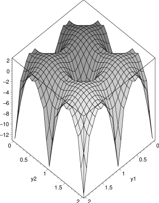
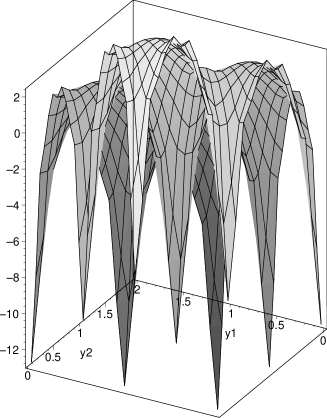
Figure 4: Two views of the effective potential for the inflaton field in a two dimensional torus transverse to the branes. The periods of the lattice are normalised to 1 in both directions. Notice how the rotational symmetry is recovered close to the brane.

For distances much larger than the string scale $y\gg l_{s}$, the terms that contribute most to the integral are those that appear in the limit $t\rightarrow 0$. In that limit, the partition function (10) becomes $Z(\theta,t)\rightarrow 4\,t^{3}\,\sin^{2}\theta/2\,\tan\theta/2$, and the potential, for $l_{s}\ll y_{i}\ll 2\pi R_{i}$, can be approximated by:

$$V(y)=2T_{4}L-\,{\sin^{2}\theta/2\,\tan\theta/2\over 8\pi^{3}\alpha^{\prime}y^{2}}\,.$$ (12)

This potential has the expected form, with the right power of the distance, as could be deduced from Gauss law, i.e. from the exchange of massless fields in $d_{\bot}=4$ transverse dimensions. We have plotted this potential in Fig. 5 for the case of $\theta=\pi/12$.

The brane-antibrane system of Refs. [13, 14] is the extreme case of two branes with opposite orientations. The brane and antibrane attract each other with a force that depends on the distance [20]:

$$V(y)=2T_{p}L-{B\over y^{d_{\bot}-2}}\,,$$ (13)

where $B$ is a positive constant of order one in string units, and $d_{\bot}=9-p$ is the number of transverse dimensions to the branes. In the brane-antibrane system, due to the strong force between them, one has to chose a special location for the branes in order to have enough number of $e$-folds . In our case, as we will show, the number of $e$-folds is not so sensitive to the location of the branes, as long as the angle is sufficiently small.

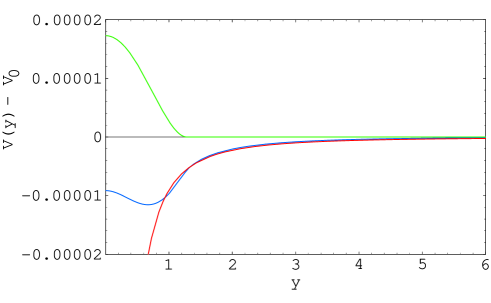
Figure 5: The attractive inflaton potential between two D4-branes. The red line corresponds to the string-derived potential (12); in blue is the Real part of the Coleman-Weinberg field-theory limit of the same potential (48), and in green is the Imaginary part, which is non-zero only when the tachyon condenses, at $y^{2}<2\pi\alpha^{\prime}\theta$. We have chosen here $\theta=\pi/12$. The potential $V(y)$ and the distance $y$ are both in units of $\alpha^{\prime}=1$.

An alternative, but equivalent, way to obtain the inflaton effective action at large distances is to start in the closed string picture from the beginning and consider a probe brane moving in the supergravity background created by another BPS p-brane solution. The details of the computation for general Dp-branes are given in the Appendix A.

The resulting effective action can be organised in a perturbative expansion of small brane velocities and small supersymmetry breaking angle $\theta$. The validity of both perturbative expansions are related, since a small supersymmetry breaking induces a small brane velocity. Indeed, from the Appendix B, we can see that the ${\cal O}(v^{4})$ terms are negligible within the supergravity regime $\alpha^{\prime}/y^{2}\ll 1$. Here we just present the first $\theta$-dependent corrections to the brane probe effective action:

$$S_{\rm probe}=-(T_{4}L)\int d^{4}x\,\sqrt{-g} \left[{1\over 2}\left(1+\frac{g_{s}\pi\sin\theta}{2(M_{s}L)(M_{s}y)^{2}}\right)|\partial y|^{2}\right.$$ (14)

$$-\left.2\left(1-\frac{g_{s}\pi\tan^{3}\theta}{8(M_{s}L)(M_{s}y)^{2}}\right)\right]\,,$$

whose potential coincides precisely with Eq. (12), in the small angle approximation.

4 The inflationary scenario

In this section we will describe in some detail the constraints that a generic model of inflation in the brane, and its subsequent cosmological evolution, should satisfy in order to agree with observations. We will then use the brane inflation model described above to obtain phenomenological constraints on the parameters of the model.

4.1 Phenomenological constraints

We will give here the most relevant contraints that should be satisfied in any scenario of string brane inflation and its subsequent cosmology. For reviews see [1, 2, 31].

1. Inflation should be possible, i.e. the energy density of the universe should be such that the scale factor accelerates: $\ddot{a}/a>0$, or, in terms of the rate of expansion $H=\dot{a}/a$, we should have $\epsilon=-\dot{H}/H^{2}<1$.

2. Sufficient number of $e$-folds during inflation, $N=\ln(a_{\rm end}/a_{\rm ini})$, in order to solve the horizon and flatness problems. This constraint depends on the scale of inflation. In order for the universe to be essentially flat, with $\Omega_{0}=1.0\pm 0.1$, we require $(\Omega_{0}-1)/\Omega_{0}=\exp(-2N)(T_{\rm rh}/T_{\rm eq})^{2}\,(1+z_{\rm eq})\simeq 0.1$, which implies

   $$N\geq 54+\ln\Big{(}{T_{\rm rh}\over 10^{12}\,{\rm GeV}}\Big{)}\,.$$ (15)

   For the case of GUT-scale inflation, one needs $N\geq 60$, while for EW-scale inflation, $N\geq 34$, where the number of $e$-folds is computable in terms of the variations in the scalar field that drives inflation,

   $$N=\int Hdt={1\over M_{\rm P}^{2}}\int_{\phi_{e}}^{\phi_{N}}{V(\phi)\,d\phi\over V^{\prime}(\phi)}\,,$$ (16)

   with $M_{\rm P}=(8\pi G)^{-1/2}=2.4\times 10^{18}$ GeV the Planck mass.

3. Amplitude and tilt of scalar density perturbations and the induced temperature anisotropies of the microwave background. Quantum fluctuations during inflation leave the horizon and imprint classical curvature perturbations on the metric, which later (during radiation and matter eras) enter inside our causal horizon, giving rise through gravitational collapse to the large scale structure and the observed temperature anisotropies of the cosmic microwave background (CMB).

   The slow-roll parameters are defined as

   $$\epsilon = {M_{\rm P}^{2}\over 2}\Big{(}{V^{\prime}(\phi)\over V(\phi)}\Big{)}^{2}\ll 1$$ (17)

   $$\eta = M_{\rm P}^{2}{V^{\prime\prime}(\phi)\over V(\phi)}\ll 1$$ (18)

   The density contrast ($\delta={\delta\rho\over\rho}$) and the scalar tilt at horizon satisfy [32, 33]

   $$\delta_{H} = {2\over 5}{\cal P}_{\cal R}^{1/2}={1\over 5\pi\sqrt{3}}{V^{3/2}(\phi)\over V^{\prime}(\phi)M_{\rm P}^{3}}=1.91\times 10^{-5}\,,\hskip 28.45274pt90\%\ {\rm c.l.}$$ (19)

   $$n-1 = {\partial\ln{\cal P}_{\cal R}(k)\over\partial\ln k}\simeq 2\eta-6\epsilon\,,\hskip 28.45274pt|n-1|<0.10\,,\hskip 28.45274pt90\%\ {\rm c.l.}$$ (20)

4. Amplitude and tilt of gravitational waves. Not only scalar curvature perturbations are produced, but also transverse traceless tensor fluctuations (gravitational waves), with amplitude and tilt:

   $${\cal P}_{g}^{1/2} = {\sqrt{2}\over\pi}{H\over M_{\rm P}}<10^{-5}\hskip 56.9055pt{\rm CMB\ bound}\,,$$ (21)

   $$n_{T} = {\partial\ln{\cal P}_{g}(k)\over\partial\ln k}\simeq-2\epsilon\ll 1\hskip 28.45274pt{\rm(not\ yet\ observed).}$$ (22)

5. Graceful exit. One must end inflation and enter the radiation dominated era. This typically occurs by the end of slow-roll, like in the usual chaotic inflation models [1], when $\epsilon_{\rm end}=1$, and not when $\eta_{\rm end}=1$, as incorrectly stated in the literature. One should then compute the number of $e$-folds from this time backwards, to see if there are sufficient $e$-folds to solve the horizon and flatness problems.

   A different way to end inflation is through its coupling to a tachyonic (Higgs) field, where the spontaneous symmetry breaking triggers the abrupt end of inflation, like in hybrid inflation [34]. This allows for $\epsilon_{\rm end}\ll 1$.

6. Reheating before primordial nucleosynthesis. Reheating is the most difficult part in model building since we don’t know to what the inflaton couples to. Eventually one hopes everything will thermalise and the hot Big Bang will start. One thing we know for sure is that the universe must have reheated before primordial nucleosynthesis ($T_{\rm rh}>1$ MeV), otherwise the light element abundances would be in conflict with observations. However, since the scale of inflation is not yet determined observationally, we are allowed to consider reheating the universe just above a few MeV.

7. The matter-antimatter asymmetry of the universe. The universe is asymmetric with respect to baryon number, and the decays of the inflaton field typically conserve Baryon number, so it remains a mystery how the baryon asymmetry of the universe came about. According to Sakharov, we need B-, C- and CP-violating interactions out of equilibrium. The first three occur in the Electroweak theory, but we would need to reheat the universe above 100 GeV, which may be too demanding, unless the fundamental Planck scale (in this case the string scale) is relatively high.

8. The diffuse gamma ray background constraints. If reheating occurs by emission of massless states to the bulk as well as into the brane, one must be sure that the bulk gravitons do not reheat at too high a temperature, because their energy does not redshift inside the large compact dimensions (contrary to our (3+1)-dimensional world, where radiation redshifts with the scale factor like $a^{-4}$), and they could interact again with our (presently cold) brane world and inject energy in the form of gamma rays, in conflict with present bounds from observations of the diffuse gamma ray background [35].

9. Model dependent constraints. In the case of brane inflation models with large extra dimensions one may prefer that the low energy effective field theory remains (3+1)-dimensional (otherwise the cosmological evolution in the brane has to take into account the evolution of the extra dimensions). In that case, the Hubble scale should be much larger than the compactification scale, $H\,R\ll 1$. This does not impose any serious constraint, in general. Also, in order to prevent fundamental couplings from evolving during or after inflation we require that the moduli fields of the compactified space be fixed.

4.2 The model of brane inflation

Figure 6: Two D4-branes attract each other to decay in the last step to a bound state. The inflation process will take place when the two branes are far away if the angle between the two branes is small enough. Note that we have chosen here $\theta=\pi/2$ for pictorical purposes. In fact the branes are at an angle $\theta\ll 1$, so we would expect the final brane to be wrapped around the corresponding cycle.

We will consider here a concrete brane model based on two D4-branes separated by a distance $y$, and intersecting at a small angle $\theta$, which attract each other due to the soft supersymmetry breaking induced by this angle, see Fig. 6. As previously mentioned, we consider that all the closed string moduli are frozen out. We are also ignoring the effect of the relative velocity of the branes, which would introduce a correction to the potential proportional to the fourth power of the speed. We have computed these corrections in Appendices A and B, and we have confirmed that they are negligible for our model. They can be computed to all order in $\alpha^{\prime}$ from the one-loop open string channel. At long distances, only the massless closed string modes contribute to these corrections, i.e. the supergravity approach is reliable. At short distances, only high speed effects are important, and they are bigger if the angle between the two branes is small. But the process of inflation we are considering occurs at very low velocity and long distances. As we will see below, the velocity is related to the slow-roll parameter $\epsilon$, which in our case is very small. The corrections are therefore negligible. These effects are very important when the distance between the two branes is of the order of the string scale, then the speed contributions are the dominant ones.

The 4-dimensional effective action can be written as

$$S=\int d^{4}x\,\sqrt{-g}\Big{[}{1\over 2}M_{\rm P}^{2}\,R-{1\over 2}T_{4}L(\partial_{\mu}y)^{2}+V(y)\Big{]}\,,$$ (23)

where $M_{\rm P}^{2}=M_{s}^{2}(2\pi R\,M_{s})^{6}g_{s}^{-2}\$ is the 4-dimensional Planck mass, and $R$ is related to the compactification volume as $V_{6}=(2\pi R)^{6}$. The potential (12) for the canonically normalised inflaton field, $\psi=(T_{4}L)^{1/2}y$, is given by

$$V(\psi)=M^{4}\Big{(}1-\beta\,{M_{s}^{2}\over\psi^{2}}\Big{)}\,,$$ (24)

where $M^{4}\equiv 2T_{4}L=2(2\pi)^{-4}M_{s}^{4}(M_{s}L)g_{s}^{-1}$, and the parameter $\beta$ is a function of the angle $\theta$ between the branes,

$$\beta={4\sin^{2}\theta/2\,\tan\theta/2\over(4\pi)^{3}}\,,$$ (25)

which is expected to be very small in order to get a sufficiently flat (slow-roll) potential.

Let us calculate the derivatives of the potential,

$$M_{\rm P}\,{V^{\prime}(\psi)\over V(\psi)} \simeq 2\beta\,{M_{\rm P}\over M_{s}}\,{M_{s}^{3}\over\psi^{3}}\,,$$ (26)

$$M_{\rm P}^{2}\,{V^{\prime\prime}(\psi)\over V(\psi)} \simeq -6\beta\,{M_{\rm P}^{2}\over M_{s}^{2}}\,{M_{s}^{4}\over\psi^{4}}\,,$$ (27)

and the number of $e$-folds , (16)

$$N={1\over 8\beta}\,{M_{s}^{2}\over M_{\rm P}^{2}}\,\Big{[}{\psi^{4}\over M_{s}^{4}}-{\psi^{4}_{\rm end}\over M_{s}^{4}}\Big{]}\simeq{1\over 8\beta}\,{M_{s}^{2}\over M_{\rm P}^{2}}\,{\psi^{4}\over M_{s}^{4}}\,,$$ (28)

in terms of which we can write the slow-roll parameters (17) and (18), and the scalar tilt (20)

$$\epsilon\simeq{1\over 32N^{2}}\,{\psi^{2}\over M_{\rm P}^{2}}\,, \hskip 28.45274pt\eta\simeq-\,{3\over 4N}\,,$$ (29)

$$n \simeq 1-\,{3\over 2N}=0.974\,,$$ (30)

which is well within the present bounds from CMB anisotropies, for $N=54$. The amplitude of scalar metric perturbations (19) also gives a constraint on the model parameters,

$$\delta_{H}={N^{3/4}2^{-1/4}\over 5\sqrt{3}\pi^{3}}\,{g_{s}(M_{s}L)^{1/2}\over\beta^{1/4}(2\pi R\,M_{s})^{9/2}}=1.91\times 10^{-5}\,,$$ (31)

which implies

$$\beta^{1/4}=3.27\times 10^{3}\,{g_{s}(M_{s}L)^{1/2}\over(2\pi R\,M_{s})^{9/2}}\,,$$ (32)

and thus

$${\psi_{*}\over M_{s}}=(8\beta N)^{1/4}\,(2\pi R\,M_{s})^{3/2}\,g_{s}^{-1/2}=1.48\times 10^{4}\,{(M_{s}Lg_{s})^{1/2}\over(2\pi R\,M_{s})^{3}}\,,$$ (33)

where the asterisc denotes the time when the present horizon-scale perturbation crossed the Hubble scale during inflation, 54 $e$-folds before the end on inflation. In terms of the distance between branes, it becomes

$${y_{*}\over l_{s}} = {5.88\times 10^{5}\,g_{s}\over(2\pi R\,M_{s})^{3}}\,,$$ (34)

$${y_{*}\over 2\pi R} = {5.88\times 10^{5}\,g_{s}\over(2\pi R\,M_{s})^{4}}\,,$$ (35)

so a compactification radius of order $2\pi R\,M_{s}=60$ gives, for $g_{s}=0.1$, i.e. in the weak string coupling regime,

$$l_{s}<2.3\ l_{s}=y_{*}={2\pi R\over 14}\ll 2\pi R$$

and $\beta^{1/4}=7.4\times 10^{-6}\,(M_{s}L)^{1/2}$, which could be made somewhat larger by chosing a large wrapping length $L$ of the brane around the cycle in the compactified space, e.g. $LM_{s}\sim 200$, or $\beta^{1/4}\sim 10^{-3}$, in which case the angle for supersymmetry breaking is $\theta=2\times 10^{-3}$. This small angle ensures that inflation will end, triggered by the tachyon field, when $y\leq y_{c}=0.1\ l_{s}$. This value of the compactification radius, $2\pi R\,M_{s}=60$, gives a string scale, a Hubble rate and a scale of compactification

$$M_{s} = M_{\rm P}\,(2\pi R\,M_{s})^{-3}\,g_{s}\simeq 9\times 10^{12}\ {\rm GeV}\,,$$ (36)

$$M = (2M_{s}L\,g_{s}^{-1})^{1/4}{M_{s}\over 2\pi}\simeq 1\times 10^{13}\ {\rm GeV}\,,$$ (37)

$$H = {M^{2}\over\sqrt{3}M_{\rm P}}\simeq 3\times 10^{7}\ {\rm GeV}\,,$$ (38)

$$R^{-1} = 2\times 10^{12}\ {\rm GeV}\,.$$ (39)

Let us now study the production of gravitational waves with amplitude (21),

$${\cal P}_{g}^{1/2}={4\over\sqrt{3}(2\pi)^{3}}\,{(M_{s}Lg_{s}^{-1})^{1/2}\over(2\pi R\,M_{s})^{6}}=6\times 10^{-10}\,,$$ (40)

which is well below the present bound (21).

Finally we may ask whether our approximation of using a 4-dimensional effective theory is correct. For that we need to have the Hubble radius, $H^{-1}$, of the 4D theory during inflation much larger than the compactified dimensions,

$$H\,R={\sqrt{2}\over(2\pi)^{3}}\,{(M_{s}Lg_{s}^{-1})^{1/2}\over(2\pi R\,M_{s})^{2}}=1.5\times 10^{-5}\,,$$ (41)

so we are indeed safely within an effective 4D theory.

4.3 Geometrical interpretation of brane inflation parameters

Figure 7: The dilaton field $y$ is interpreted as the distance between the two branes. Quantum fluctuations of this field will give rise upon collision to density perturbations on comoving hypersurfaces. These fluctuations will be later observed as temperature anisotropies in the microwave background.

Here we will give a geometrical interpretation of the number of $e$-folds and the slow-roll parameters in our model. The epsilon parameter (17) is in fact the relative squared velocity ($v=\dot{y}$) of the branes in the compact dimensions. Since $\dot{\psi}^{2}=M^{4}v^{2}/2$ and $3H^{2}=M^{4}/M_{\rm P}^{2}$, we have

$$\epsilon=-{\dot{H}\over H^{2}}={\dot{\psi}^{2}\over 2M_{\rm P}^{2}H^{2}}={3\over 4}\,v^{2}\,.$$ (42)

The number of $e$-folds (16) can be seen to be proportional as the distance between the branes in the compactified space,

$$N=\int{d\psi\over M_{\rm P}\sqrt{2\epsilon}}={H\over v}\,\int dy\,.$$ (43)

Finally, the eta parameter (18) is the acceleration of the branes with respect to each other due to an attractive potential of the type $V(y)\propto y^{2-d_{\bot}}$, coming from Gauss law in $d_{\bot}$ transverse dimensions,

$$\eta=-{d_{\bot}-1\over d_{\bot}\,N}\,,$$ (44)

which only depends on the dimensionality of the compact space $d_{\bot}$. Note that the spectral tilt of the scalar perturbations (20) therefore depends on both the velocity and acceleration within the compact space, and is very small in our model of spontaneous supersymmetry breaking, which makes the branes approach eachother very slowly, driving inflation and giving rise to a scale invariant spectrum of fluctuations.

In fact, the induced metric fluctuations in our (3+1)-dimensional universe can be understood as arising from the fact that, due to quantum fluctuations in the approaching D4-branes, inflation does not end at the same time in all points of our 3-dimensional space, see Fig. 7, and the gauge invariant curvature perturbation on comoving hypersurfaces, ${\cal R}_{k}=\delta N_{k}=H\,\delta y_{k}/v$, is non-vanishing, being much later responsible for the observed spectrum of temperature anisotropies in the microwave background [32, 33].

5 Effective field theory description at short distances

It is important to make the matching between the superstring theory at large distances and the supersymmetric quantum field theory in the brane, whose dynamics will be important for the reheating of the universe after inflation. For that purpose, note that we can write the partition function (10) in terms of infinite products,

$$Z(\theta,t) = {(z-1)^{4}\over z}\,\Big{(}\sum_{n=0}^{\infty}z^{2n}\Big{)}\,\prod_{m=1}^{\infty}{(1-q^{m}z)^{4}(1-q^{m}z^{-1})^{4}\over(1-q^{m})^{6}(1-q^{m}z^{2})(1-q^{m}z^{-2})}\,,$$ (45)

$$q = e^{-2\pi t}\,,\hskip 28.45274ptz=e^{-\theta t}\,.$$ (46)

The first factor, $(1-z)^{4}/z=z^{-1}-4+6z-4z^{2}+z^{3}$, gives precisely the lowest lying ${\cal N}=4$ supermultiplet, including the tachyon, see table 1 and Fig. 2, with the correct multiplicity and (bosonic/fermionic) sign. Together with the exponential factor, $\exp(-t\,y^{2}/2\pi\alpha^{\prime})$, in Eq. (9), it gives the masses for the one-loop potential

$$V_{\rm 1-loop} = {-1\over(8\pi^{2}\alpha^{\prime})^{2}}\,\int_{0}^{\infty}{dt\over t^{3}}\,\sum_{i}\,(-1)^{F_{i}}\,e^{-2\pi\alpha^{\prime}t\ m_{i}^{2}}$$ (47)

$$= {1\over 64\pi^{2}}\sum_{i}(-1)^{F_{i}}\,m_{i}^{4}\,\log\,m_{i}^{2}\,,$$ (48)

which corresponds to the Coleman-Weinberg potential for the low energy effective field theory. The fact that $\sum_{i}(-1)^{F_{i}}\,m_{i}^{2n}=0,\ (n=1,2,3)$, ensures that (47) is finite, as it should be, since supersymmetry is being spontaneously broken.

We can then consider the next series of states in (45). The factor $\sum_{n=0}^{\infty}z^{2n}=1+z^{2}+z^{4}+z^{6}+\dots$ corresponds to the Landau levels induced, in the dual picture, by the supersymmetry breaking flux associated to the angle $\theta$. They give, at any order $N$, a supermultiplet with $\sum_{i}(-1)^{F}\,m_{i}^{2n}=0,\ (n=1,2,3)$, so they still provide a finite one-loop potential (48). For a given supersymmetry-breaking angle $\theta$, one should include in the low energy effective theory the whole tower of Landau levels up to $N=1/\theta$. For instance, the spectrum for $\theta=\pi/2$ is derived from $(1-z)^{4}/z\,(1+z^{2}+z^{4})=z^{-1}-4+7z-8z^{2}+8z^{3}-8z^{4}+7z^{5}-4z^{6}+z^{7}$, with masses given by Table 2.

Field	$2\pi\alpha^{\prime}m^{2}-\frac{y^{2}}{2\pi\alpha^{\prime}}$
1 scalar	$7\theta$
2 massive fermions	$6\theta$
3 scalars	$5\theta$
2 massive gauge fields	$5\theta$
4 massive fermions	$4\theta$
4 scalars	$3\theta$
2 massive gauge fields	$3\theta$
4 massive fermions	$2\theta$
3 scalars	$\theta$
2 massive gauge fields	$\theta$
2 massive fermions (massless for $y=0$)	$0$
1 scalar (tachyonic for $y=0$)	$-\theta$

Table 2: The mass spectrum of the lowest 3 Landau levels, which fall into ${\cal N}=4$ supermultiplets.

Finally, one could include also the first low-lying string states, whose masses are determined by the expansion of the infinite products in (45),

$$Z(\theta,t)={(z-1)^{4}\over z}\,\Big{(}\sum_{n=0}^{\infty}z^{2n}\Big{)}\,\Big{[}1+{(1-z)^{4}\over z^{2}}\,q^{2}+{(1-z)^{4}(1+7z^{2}+z^{4})\over z^{4}}\,q^{4}+\dots\Big{]}\,.$$ (49)

Their structure still comes in ${\cal N}=4$ supermultiplets, so they again give a finite Coleman-Weinberg potential (48).

We will use the whole tower of Landau levels in the effective field theory to connect the one-loop potential at short distances, determined by the Coleman-Weinberg potential (48), with the full string theory one-loop potential coming from exchanges of the massless string modes at large distances, responsible for inflation. This connection will be essential for the latter stage of preheating and reheating, because it will provide the low energy effective masses, and the couplings between the inflaton field $y$ and the effective fields living on the D4-brane.

The potential (47) is finite if there are no massless or tachyonic fields. When the tachyon appears, i.e. at distances smaller tham $y_{c}$, there is an exponentially divergent amplitude for $m_{i}<0$. A possible strategy to attach physical meaning to this divergence is to analytically continue the potential (9) in the complex $y$-plane. After the continuation, there is a logarithmic branch point at $y=y_{c}$. In this way, we get rid of the divergence and the potential develops a non-vanishing imaginary part for $y<y_{c}$, which signals the instability of the vacuum.

We have plotted in Fig. 5 the attractive potential $V(y)$ between two D4-branes at an angle $\theta=\pi/12$. The large distance behaviour $y^{2}\gg\alpha^{\prime}$ is determined from the supergravity amplitude (12), in red, while the short distance potential is obtained from the Coleman-Weinberg potential corresponding to the lowest-lying effective fields, which fall into ${\cal N}=4$ supermultiplets. The real part of the Coleman-Weinberg potential is drawn in blue in Fig. 5, while the imaginary part is in green.

In the field theory limit ($q\to 0$ and $z\neq 0$) we can consider the infinite tower of Landau levels, while ignoring the string levels, i.e. $Z(\theta,t)\simeq(z-1)^{4}\,\sum_{n=0}^{\infty}z^{2n-1}$. The finite low energy effective potential up to Landau level $N$ can be written as

$$V_{N}(y,\theta)\! = {1\over 32\pi^{2}}\,\Big{[}(y^{2}-\theta)^{2}\ln(y^{2}-\theta)-4y^{4}\ln\,y^{2}+7(y^{2}+\theta)^{2}\ln(y^{2}\!+\theta)$$

$$- 8\sum_{n=2}^{2N}(-1)^{n}(y^{2}+n\theta)^{2}\ln(y^{2}+n\theta)+7(y^{2}\!+\!(2N+1)\theta)^{2}\ln(y^{2}\!+\!(2N+1)\theta)$$

$$- 4(y^{2}\!+\!(2N+2)\theta)^{2}\ln(y^{2}\!+\!(2N+2)\theta)+(y^{2}\!+\!(2N+3)\theta)^{2}\ln(y^{2}\!+\!(2N+3)\theta)\Big{]}$$

where $y$ stands for $y/(2\pi\alpha^{\prime})$ and $\theta$ for $\theta/(2\pi\alpha^{\prime})$.

From this expression we can compute what is the value of the potential at the distance $y=0$; we expect the tachyon to give an imaginary contribution to the vacuum energy, which could be interpreted as the rate of decay of the false vacuum towards the minimum of the tachyon potential. On the other hand, the real part can be summed over,

$$V_{N}(0,\theta) = {1\over 32\pi^{2}}\,\Big{[}i\pi-8\sum_{n=2}^{2N}(-1)^{n}n^{2}\ln(n)+7(2N+1)^{2}\ln(2N+1)$$

$$- 4(2N+2)^{2}\ln(2N+2)+(2N+3)^{2}\ln(2N+3)\Big{]}\left({\theta\over 2\pi\alpha^{\prime}}\right)^{2}\,.$$

The infinite sum converges in the limit $N\to\infty$ to:

$$V_{\infty}(0,\theta)={i\pi-1.70638\over 32\pi^{2}}\,\left({\theta\over 2\pi\alpha^{\prime}}\right)^{2}\,.$$ (52)

This quantity corresponds to the difference between the false vacuum energy at large distances between the branes, $E_{0}=2T_{p}L$, and the height of the tachyon potential at zero distance ($y=0$), and should be compared with $\Delta V_{\rm tachyon}$ in Eq. (8), the difference between $E_{0}$ and the final energy density in the tachyonic vacuum $E_{f}$. Both are proportional to $\theta^{2}$, as expected, since at $y=0$ the one-loop potential (47) in the field theory limit $q\to 0$ can be written as

$${-1\over(8\pi^{2}\alpha^{\prime})^{2}}\,\int_{0}^{\infty}{dt\over t^{3}}\,{(1-z)^{4}\over z}\,\sum_{n=0}^{\infty}z^{2n}=-\Big{(}{\theta\over 8\pi^{2}\alpha^{\prime}}\Big{)}^{2}\,\int_{0}^{\infty}{du\over u^{3}}\,e^{u}\,(1-e^{-u})^{4}\,\sum_{n=0}^{\infty}e^{-2nu}\,.$$ (53)

What we have done to obtain (52) is to regularise this integral, for instance introducing a mass cut-off, to make it absolutely convergent and then commute it with the sum. The fact that the one-loop effective action is finite for each Landau level allows us to send the cut-off to infinity such that only the series (5) remains.

Figure 8: A sketch of the inflaton-tachyon potential $V(T,y)$. The flat region corresponds to the inflationary regime.

We have to compare the two quantities:

$$\Delta V_{\infty} = {1.70638\over 32\pi^{2}}\,\left({\theta\over 2\pi\alpha^{\prime}}\right)^{2}\,,$$ (54)

$$\Delta V_{T} = {2M_{s}Lg_{s}^{-1}\over 32\pi^{2}}\,\left({\theta\over 2\pi\alpha^{\prime}}\right)^{2}\,,$$ (55)

in the small angle approximation. In order to ensure that the tachyon minimum is a global minimum for the low-energy effective theory, we need $M_{s}L>0.8352\,g_{s}$, which is easy to accommodate within the model. A sketch of the potential in both inflaton and tachyon directions is shown in Fig. 8. The dotted line indicates where inflation ends and the tachyon instability sets in.

Note that after both branes collide, a vacuum energy density remains, which, for small angles, is of the same order as the original $V_{0}$. The cancellation of this energy density depends on the expectator branes/orientifolds necessary to cancel the R-R tadpoles and is irrelevant for the period of inflation, but should be taken into account at reheating.

6 Preheating and reheating

In this section we will briefly describe reheating after inflation, i.e. the mechanism by which the inflaton potential energy density gets converted into a thermal bath at a given temperature. The details of reheating lie somewhat out of the scope of the present paper. We will give here a succint account of what should be expected and leave for the next paper a more detailed description.

Inflation ends like in hybrid inflation, still in the slow-roll regime, when the string-tachyon becomes massless and the tachyon symmetry is broken immediately after. In Ref. [36] it was shown that this typically occurs very fast, within a time scale of order the inverse curvature of the tachyon potential, $t_{*}\sim m_{T}^{-1}\equiv(\theta/2\pi\alpha^{\prime})^{-1/2}$. From the point of view of the low energy effective field theory description, this is seen as the decay rate (per unit time and unit volume) or the imaginary part of the one-loop energy density (52).

Assuming that the false vacuum energy $E_{0}\simeq 2T_{p}L=M^{4}$ of the two branes is all of it eventually converted into radiation, we can compute the reheating temperature of the universe as

$$T_{\rm rh}\simeq\Big{(}{30\over\pi^{2}g_{*}}\Big{)}^{1/4}\,M=2.2\times 10^{12}\ {\rm GeV}\,,$$ (56)

where we have taken $g_{*}\sim 10^{3}$ for the number of relativistic degrees of freedom at reheating, and we have neglected the energy lost in the expansion of the universe from the end of inflation to the time of reheating, since the rate of expansion at the end of inflation $H\sim M^{2}/\sqrt{3}M_{\rm P}$ is negligible compared with $m_{T}$.

The actual process of reheating is probably very complicated and there is always the possibility that some fields may have their occupation numbers increased exponentially due to parametric resonance [37] or tachyonic preheating [36]. Moreover, a significant fraction of the initial potential energy may be released in the form of gravitational waves, which will go both to the bulk and into the brane. Fortunately, since the fundamental gravitational scale, $M_{\rm P}$, in this model is large enough compared with all the other scales, the coupling of those bulk graviton modes to the brane is suppressed, so we do not expect any danger with the diffuse gamma ray background [35], but a detailed study remains to be done.

7 Conclusions

In this paper, we have analysed the realisation of inflationary models arising from the dynamics of D-branes departing only slightly from a supersymmetric configuration. The inflaton field is realised in these models as the inter-brane distance within a compact space transverse to the branes. As a first example, we obtained the effective interaction potential for the inflaton field in the case of two almost parallel D4-branes. Due to the small supersymmetry breaking, the potential is almost flat, and therefore satisfies the slow-roll conditions. It is also interesting to point out the geometrical interpretation for various other cosmological parameters, such as the number of $e$-folds , or the slow-roll parameters $\epsilon$ and $\eta$, as well as the quantum fluctuations that give rise to CMB anisotropies.

We have analysed the period of inflation in detail within the supergravity regime. Both D-branes attract each other with a small velocity at distances much larger than the string scale, but still much smaller than the compactification scale. In this way, the process involved is essentially local, without much dependence on the type of compactification. We find that a sufficient number of $e$-folds to solve the flatness and horizon problems can easily be accommodated within the model. For a concrete compactification radius in units of the string scale, $2\pi R=60\ l_{s}$, we find a mass scale $M\sim M_{s}\sim 10^{13}$ GeV. Moreover, the radius of compactification turns out to be $R^{-1}\sim 10^{12}$ GeV. An account of the reheating mechanism after inflation remains to be studied in detail, and in particular the ratio of energy which is radiated to the bulk versus that into the brane.

A nice feature of the model is the fact that the tachyonic instability inherent to the brane model triggers the end of inflation. Since the D4-branes wrap different non-trivial homology cycles, a single supersymmetric D4-brane remains after both branes collide. We analysed the brane interaction at short distances by taking the effective field theory description on the brane. We computed the Coleman-Weinberg potential and obtained a good matching with the supergravity potential. It remains to study the reheating involved in this regime. We believe that since the supersymmetry breaking on the brane field theory is small, maybe it will be possible to study the interactions of the tachyon with other fields by standard supersymmetric field theory methods.

There are a series of important issues which should be analysed [38]: i) The first issue is the cancellation of the R-R tadpoles. Since the branes move in a compact space, the total R-R charge should vanish. We can put another D4-brane, wrapping the final cycle with opposite orientation, or an orientifold plane with exactly the same opposite R-R charge, far away from the two branes driving inflation, such that during the period of inflation and the reheating of the universe, this extra brane is an expectator where the R-R flux can end. ii) The second issue is the moduli stabilisation. There is a non-supersymmetric back-reaction on the bulk, as well as non-zero NS-NS tadpoles, that produces a non-trivial temporal evolution for the closed string moduli, such us the dilaton and the compactification radii. The idea is that the time scale involved for this process is much larger than the time involved during inflation and reheating. One can compute the tadpoles by taking the square root of the annulus amplitude. In general terms, the tadpoles are proportional to $\sqrt{V_{\parallel}/V_{\perp}}$, where $V_{\parallel}$ and $V_{\perp}$ are the volumes of the compact spaces parallel and perpendicular to the brane, respectively. Therefore, for large enough compactification radii, the tadpoles can be neglected. This is exactly our original configuration at the beginning of inflation, so we hope to being able to freeze the moduli, at least during the inflationary period.

Finally, note that from the general expression of the tadpole potential we can expect that the universe will naturally evolve towards decreasing both the string coupling and the parallel volume (to minimise the brane energy), while increasing the transverse volume. However, in order to precisely quantify this possibility, one would have to solve the cosmological equations of motion for this higher dimensional model. We will leave this discussion for our forthcoming publication [38].

Appendix A Probe brane effective action

Following the conventions of Ref. [25], the type II supergravity solution for an extremal Dp-brane extended in the directions $x^{\hat{\mu}}$, for $\hat{\mu}=0,1,...,p$, is

$$ds^{2}_{\rm string} =H^{-{1\over 2}}_{p}(x_{\bot})ds^{2}_{p+1}+H_{p}^{1\over 2}(x_{\bot})dx_{\bot}^{2}\,,$$ (57)

$$e^{\phi} =H_{p}^{\frac{3-p}{4}}(x_{\bot})\,,$$ (58)

$$A_{01...p} =1-H_{p}^{-1}(x_{\bot})\,,$$ (59)

with all the other supergravity fields vanishing. The function $H_{p}$ is harmonic in the $9-p$ transverse coordinates $x^{I}$, $I=p+1,...,9$, with the boundary condition $H_{p}\to 1$ for $|x_{\bot}|=\sqrt{x^{I}x_{I}}\to\infty$, in order to recover the flat Minkowski spacetime for the metric (57). Considering the rotational invariance in the transverse space, we have

$$H_{p}(|x_{\bot}|) =1+\frac{c_{p}g_{s}N}{(M_{s}|x_{\bot}|)^{7-p}}\,,$$ (60)

$$c_{p} =(2\sqrt{\pi})^{5-p}\,\Gamma(\frac{7-p}{2})\,.$$ (61)

Our case corresponds to $p=4$ and $N=1$ (number of background branes), but to stress the generality of this technique, we shall keep $p<7$ and $N$ arbitrary.

The effective action for a probe Dp-brane moving in this background is given by

$$S_{\rm p-brane} =S_{\rm BI}+S_{\rm WZ}\,,$$ (62)

$$S_{\rm BI} =-T_{p}\int_{\rm Dp}d^{p+1}\xi\ e^{-\phi}\sqrt{-{\rm det}(G_{MN}(X)\partial_{\mu}X^{M}\partial_{\nu}X^{N})}\,,$$ (63)

$$S_{WZ} =-T_{p}\int_{\rm Dp}A_{5}\,.$$ (64)

We take the configuration for the probe rotated in the $\{x^{p},x^{p+1}\}$ plane:

$$X^{\mu}=\xi^{\mu}\,,\hskip 56.9055pt\mu=0,1,...,p-1\,,$$

$$X^{p}=\xi^{p}\cos\theta\,,$$

$$X^{p+1}=\xi^{p}\sin\theta\,,$$

$$X^{I}=y^{I}(\xi^{\mu})\,,\hskip 42.67912ptI=p+2,...,9\,.$$ (65)

Plugging into (62), we obtain

$$S_{\rm BI}= -T_{p}\cos\theta\int d^{p}x\,d\xi^{p}\sqrt{-g}\ H_{p}^{-1}\sqrt{1+H_{p}\tan^{2}\theta}\sqrt{{\rm det}(\delta^{\mu}_{\nu}+H_{p}\partial^{\mu}y^{I}\partial_{\nu}y_{I})}\,,$$ (66)

$$S_{\rm WZ}= -T_{p}\cos\theta\int d^{p}x\,d\xi^{p}\,\sqrt{-g}\ (1-H_{p}^{-1})\,,$$ (67)

There are two conditions in order to have that the brane probe action (62) is a valid approximation for the effective action of the inflaton field. The first is that the supersymmetry breaking mass scale is small with respect the string and Plank scales, to aboid relevant supersymmetry-breaking back-reaction effects on the background. In our model, supersymmetry is spontaneously broken by the rotated brane configuration (65). For sufficiently small angle, we can take the non-supersymmetric back-reaction as a sub-leading effect, at least in the region of small curvature.

This brings us to the second condition, which is to use the action (62) only in the valid supergravity regime. It corresponds to large inter-brane distances with respect to the string length, i.e. $M_{s}|x_{\bot}|\gg 1$, in order to neglect the massive stringy effects. Later on, we will see that small angle allows us to treat the inflationary period within the supergravity regime, such that both conditions are satisfied. For the analysis of preheating, when $M_{s}|x_{\bot}|\sim 1$ and the tachyon is turned on, massive closed string states become relevant and one should follow a different strategy to describe the relevant degrees of freedom. We leave the quantitative analysis of preheating for the future [38].

Notice that the two above mentioned conditions, $\theta/\pi$ and $(M_{s}|x_{\bot}|)^{-1}$ much smaller than one, correspond to the two natural expansion parameters for the probe action (62). We can perform an expansion for the first square-root factor in (66) of the form

$$\cos\theta\sqrt{1+H_{p}\tan^{2}\theta}=\sqrt{1+I_{p}}=1+\frac{I_{p}}{2}-\frac{I_{p}^{2}}{8}+{\cal O}(I_{p}^{3})\,,$$ (68)

where we have defined

$$I_{p}=\sin^{2}\theta\frac{c_{p}g_{s}N}{(M_{s}|x_{\bot}|)^{7-p}}\ll 1\,.$$ (69)

For the second square-root in (66), we can expand with respect small velocities, or what is the same, in the gradient $K^{\mu}_{\nu}=\partial^{\mu}y^{I}\partial_{\nu}y_{I}$, of the form

$$\sqrt{1+H_{p}K}=1+H_{p}{\rm tr}K+\frac{H_{p}^{2}}{4}\left({1\over 2}({\rm trK)}^{2}-{\rm tr}(K^{2})\right)+{\cal O}(K^{3})\,.$$ (70)

The result is that we can organise the kinetic and potential terms for the inflaton in a perturbative expansion in $\theta/\pi$ and inverse powers of $(M_{s}|x_{\bot}|)$:

$$S_{\rm p-brane}=\int_{\rm R^{1,p-1}}d^{p}x\,\sqrt{-g}\ ({\cal L}_{K}(y)-V(y))\,,$$ (71)

with the kinetic terms given by

$${\cal L}_{K}(y)=-T_{p} \int_{0}^{L}d\xi^{p}\ \left(1+{1\over 2}I_{p}(y,\xi^{p})-\frac{1}{8}I_{p}^{2}(y,\xi^{p})+...\right)$$

$$\times \left({1\over 2}{\rm tr}K(y)+\frac{H_{p}(y,\xi^{p})}{4}\left({1\over 2}({\rm tr}K(y))^{2}-{\rm tr}(K^{2}(y))\right)+...\right)\,,$$ (72)

and the potential terms given by

$$V(y)=T_{p}\cos\theta\int_{0}^{L}d\xi^{p}\left(1+{1\over 2}\tan^{2}\theta-\frac{1}{8}H_{p}(y,\xi^{p})\tan^{4}\theta+...\right)\,.$$ (73)

Since the brane probe is rotated with respect the brane background, the harmonic function $H_{p}$ (and consequently $I_{p}$ also) depends on the world-volume coordinate $\xi^{p}$ through the combination $|x_{\bot}|=\sqrt{y^{2}+\xi_{p}^{2}\sin^{2}\theta}$. This longitudinal Dp-brane direction is wrapping a non-trivial cycle in the toric plane $\{x^{p},x^{p+1}\}$. If we consider a squared torus with size $4\pi^{2}R_{\bot}^{2}$, then the lenght of the cycle is $L=2\pi R_{\bot}/\sin\theta$. Notice that we can also include the corrections due to a finite compactification scale in the remaining transverse coordinates, $X^{I}$ for $I=p+2,...,9$, by just replacing the expression of the harmonic function $H_{p}$ in (60) by its corresponding Kaluza-Klein expression. We can look at the Appendix C for a discussion on this. Again, they will be small if we can keep our analysis for an inter-brane distance smaller than the compactification scale.

As an illustrative example, let us compute the first non-supersymmetric corrections to the effective action of the inflaton. Form (72), the first correction to the kinetic energy comes from the integral

$${1\over 2}\int_{0}^{\infty}d\xi^{p}\ I_{p}(y,\xi^{p}) =\frac{\sin\theta c_{p}g_{s}N}{2M_{s}}\int_{0}^{\infty}dx\left(M_{s}^{2}y^{2}+x^{2}\right)^{\frac{p-7}{2}}$$ (74)

$$=\frac{c_{p+1}g_{s}N}{(M_{s}y)^{6-p}}\frac{\pi\sin\theta}{2M_{s}}\,.$$

In this case we have for the kinetic term

$${\cal L}_{K}=-\frac{T_{p}L}{2}\left(1+\frac{\pi\sin\theta}{2M_{s}L}\frac{c_{p+1}g_{s}N}{(M_{s}y)^{6-p}}+...\right)|\partial y|^{2}\,,$$ (75)

and for the potential energy,

$$V(y)=T_{p}L\left(1-\frac{\pi\tan^{3}\theta}{8M_{s}L}\frac{c_{p+1}g_{s}N}{(M_{s}y)^{6-p}}+...\right)\,,$$ (76)

For $p=4$, $N=1$ and small angles $\theta\ll\pi$, it gives exactly half of Eq. (12). This should be expected, since we have only considered one probe brane, and we have not introduced, for instance, the rest energy of the other.

Appendix B Velocity-dependent corrections to the inflaton potential.

The corrections due to the speed of the branes can be obtained very easily from the one-loop open string amplitude (or equivalently by the tree level exchange of closed strings) by considering two angles. The first angle is our $\theta$, the second one can be taken to be imaginary and corresponds to the hyperbolic tangent of the speed. This procedure is described in detail in [25]. The potential at long distances has a dependence with the velocity of the form:

$$V(y,v)={-1\over 16\pi^{3}\alpha^{\prime}r^{2}}\frac{(\cos{\theta}-\gamma)^{2}}{\gamma\sin{\theta}}\,,$$ (77)

where $r^{2}=y^{2}+\tau^{2}v^{2}$ is the distance between the two branes and $\gamma$ is the relativistic factor: $\gamma=1/\sqrt{1-v^{2}}$. The same expresion can be obtained from the probe brane effective action (71) at leading order in $\alpha^{\prime}/y^{2}$. Notice also that this potential is invariant $v\rightarrow-v$, as expected from time reversal.

One can expand the above expression in the low speed limit to get the corrections to the static potential from the motion of the branes:

$$\frac{(\cos{\theta}-\gamma)^{2}}{\gamma\sin{\theta}} = \frac{(\cos{\theta}-1)^{2}}{\sin{\theta}}+\frac{v^{2}}{2}\sin\theta-\frac{v^{4}}{8}\frac{(\cos^{2}\theta-3)}{\sin\theta}+{\cal O}(v^{6})\,.$$ (78)

The first term is just the static interaction:

$$V(y,0)={-1\over 16\pi^{3}\alpha^{\prime}r^{2}}\frac{(\cos{\theta}-1)^{2}}{\sin{\theta}}=\frac{-1}{8\pi^{3}\alpha^{\prime}r^{2}}\sin^{2}{\theta\over 2}\,\tan{\theta\over 2}\,.$$ (79)

The second term is the correction to the inflaton kinetic term:

$$V_{2}(y,v)=\frac{-1}{32\pi^{3}\alpha^{\prime}r^{2}}\sin\theta\,.$$ (80)

This correction vanishes in the supersymmetric case when the two branes become parallel [25]. The fourth order correction is:

$$V_{4}(y,v)=\frac{-1}{128\pi^{3}\alpha^{\prime}r^{2}}\frac{(3-\cos^{2}\theta)}{\sin\theta}\,.$$ (81)

Since our description of the inflationary process occurs at very low velocities we can estimate the order of magnitude of the correction due to these terms. It can be easily estimated by considering the highest speed $v$ associated with the slow-roll parameter $\epsilon$ during the inflationary process. One may worry that at low angles the sine factor in the denominator could give big corrections. Fortunately, when substituting the speed $v$ into the above formulae, one gets negligible corrections to our results.

For completeness, we can take the ultra-relativistic limit $v\rightarrow 1$. If we denote $\delta=1-v$ and expanding the above potential one gets:

$$\frac{(\cos\theta-\gamma)^{2}}{\gamma\sin\theta} = {1\over\sin\theta\sqrt{2\delta}}-2\cot\theta+{\cal O}(\sqrt{\delta})\,.$$ (82)

Notice that the interaction becomes stronger at high speeds. For a discussion about these limits, see Ref. [25].

Appendix C Discussion on compact potentials.

Within this model we are assuming that we are close enough to one of the D-branes that the effects of the other branes, as well as the effect of the winding modes around the compact space, are negligible. This means that the process we are considering is a local one, not depending very strongly on the details of the compactification and initial conditions. We will justify here this approximation.

To evaluate the importance of this approximation, we consider that the Dirichlet directions are compactified on a torus. In order to make a more general discussion let us consider $D$ Dirichlet dimensions in a torus $T^{D}$. These directions appear in the cylinder partition function as a sum over winding modes, see Eq. (10). Commuting the integral with the sum one can express the potential as a sum over the images of the brane on the torus. Thus one obtains at distances bigger than the string length an effective potential of the form:

$$V(y_{i})=\sum_{n_{i}}\frac{-k}{\Big{[}\sum_{i}(y_{i}+L_{i}n_{i})^{2}\Big{]}^{\frac{D-2}{2}}}\,,$$ (83)

where $k$ is a constant that will depend on the angles, fluxes, etc. When the system is supersymmetric the $k$ vanish, i.e. there are no interactions.

This formula is valid if the number of Dirichlet torroidal dimensions is different from two. In the case $D=2$ the integral produces a logarithmic potential. It is easy to see that the long distance behaviour is divergent and one should try to regularise the above expression. This divergence can be undertood very easily. It is due to the propagation of massless closed strings fields at long distances, i.e. an IR divergence. From the formulae below one can see that it is related to the NS-NS uncancelled tadpoles. If these tadpoles are not present one expects this divergence to disappear. That is what happens in the supersymmetric case, where the constant $k$ is zero, and in the non-compact case, where the images are not present. The computation can be done very easily by expressing the above sum as an integral:

$$V(y_{i})=\frac{-k}{\Gamma(\frac{D-2}{2})}\int_{0}^{\infty}\frac{dt}{t}\,t^{\frac{D-2}{2}}\sum_{n_{i}}e^{-t\,\sum_{i}(y_{i}+L_{i}n_{i})^{2}}\,,$$ (84)

which can be expressed, through the change of variables $t=-\pi/x$, in terms of Elliptic functions as

$$V(y_{i})=\frac{-k\,\pi^{\frac{D-2}{2}}}{\Gamma(\frac{D-2}{2})V_{T}}\int_{0}^{\infty}dx\,\prod_{i=1}^{D}\theta_{3}\Big{(}\frac{y_{i}}{L_{i}},\frac{ix}{L_{i}^{2}}\Big{)}\,,$$ (85)

where $V_{T}=\prod L_{i}$ is the volume of the torus. This expression diverges quadratically for $x\rightarrow\infty$, and can be regularised by subtracting a coordinate-independent piece in the integral. That is like subtracting an infinite constant. The regularised expression becomes

$$V(y_{i})_{\rm reg}=\frac{-k\,\pi^{\frac{D-2}{2}}}{\Gamma(\frac{D-2}{2})V_{T}}\int_{0}^{\infty}dx\,\Big{[}\prod_{i=1}^{D}\theta_{3}\Big{(}\frac{y_{i}}{L_{i}},\frac{ix}{L_{i}^{2}}\Big{)}-1\Big{]}\,.$$ (86)

By commuting again the integral and the sum one can compute the integral for each of these terms and one gets:

$$V(y_{i})_{\rm reg}=\frac{-k\,\pi^{\frac{D-2}{2}}}{\Gamma(\frac{D-2}{2})V_{T}}\sum_{m_{i}\neq 0}\ {\prod_{i}^{D}\ \cos(2\pi m_{i}y_{i}/L_{i})\over\sum_{i}^{D}\ m_{i}^{2}/L_{i}^{2}}\,,$$ (87)

where the term with all the $m_{i}=0$ has been subtracted out. Another way of interpreting this regularisation is by taking the Fourier transform of the previous one without taking into account the zero term, i.e. the infinite one. Of course, the constant term does not affect the dynamics.

References

- [1] A. D. Linde, Particle Physics and Inflationary Cosmology, Harwood Academic Press (1990); A. R. Liddle and D. H. Lyth, Cosmological inflation and large-scale structure, Cambridge University Press (2000).
- [2] D. H. Lyth and A. Riotto, Particle physics models of inflation and the cosmological density perturbation, Phys. Rept. 314 (1999) 1 [hep-ph/9807278].
-
[3]
M. Berkooz, M. R. Douglas and R. G. Leigh, Branes
Intersecting at Angles, Nucl. Phys. B 480 (1996) 265
[hep-th/9606139].
-
[4]
H. Arfaei, M.M. Sheikh Jabbari, Different D-brane
Interactions, Phys. Lett. B 394 (1997) 288
[hep-th/9608167].
M.M. Sheikh-Jabbari, Classification of Different Branes at Angles, Phys. Lett. B 420 (1998) 279 [hep-th/9710121].
R. Blumenhagen, L. Goerlich and B. Kors, Supersymmetric Orientifolds in 6D with D-Branes at Angles, Nucl. Phys. B 569 (2000) 209 [hep-th/9908130].
Supersymmetric 4D Orientifolds of Type IIA with D6-branes at Angles, HEP 0001 (2000) 040 [hep-th/9912204].
S. Forste, G. Honecker and R. Schreyer, Supersymmetric Orientifolds in 4D with D-Branes at Angles, Nucl. Phys. B 593 (2001) 127 [hep-th/0008250]. -
[5]
R. Blumenhagen, L. Goerlich, B. Kors and D. Lust,
Noncommutative Compactifications of Type I Strings on Tori with
Magnetic Background Flux, JHEP 0010 (2000) 006
[hep-th/0007024].
Magnetic Flux in Toroidal Type I Compactification, Fortsch. Phys. 49 (2001) 591 [hep-th/0010198]. - [6] R. Blumenhagen, B. Kors and D. Lust, Type I Strings with F- and B-Flux, JHEP 0102 (2001) 03 [hep-th/0012156].
-
[7]
G. Aldazabal, S. Franco, L. E. Ibañez,
R. Rabadán and A. M. Uranga, D=4 Chiral String Compactifications
from Intersecting Branes, [hep-th/0011073].
Intersecting Brane Worlds, JHEP 0102 (2001) 047, [hep-ph/0011132]. - [8] L. E. Ibañez, F. Marchesano and R. Rabadán, Getting just the Standard Model at Intersecting Branes, [hep-th/0105155].
-
[9]
M. Cvetic, G. Shiu, A. M. Uranga, Chiral
Four-Dimensional N=1 Supersymmetric Type IIA Orientifolds from
Intersecting D6-Branes, [hep-th/0107166].
Three-Family Supersymmetric Standard-like Models from Intersecting Brane Worlds, [hep-th/0107143]. - [10] R. Blumenhagen, B. Kors, D. Lust and T. Ott, The Standard Model from Stable Intersecting Brane World Orbifolds, [hep-th/0107138].
- [11] C. Bachas, A way to break supersymmetry, [hep-th/9503030].
- [12] G. Dvali, S.-H. Henry Tye, Brane Inflation, Phys. Lett. B 450 (1999) 72 [hep-ph/9812483].
- [13] G. Dvali, Q. Shafi and S. Solganik, D-brane Inflation, [hep-th/0105203].
- [14] C. P. Burgess, M. Majumdar, D. Nolte, F. Quevedo, G. Rajesh and R.-J. Zhang, The Inflationary Brane-Antibrane Universe, JHEP 0107 (2001) 047 [hep-th/0105204].
-
[15]
R. Kallosh, N=2 Supersymmetry and de Sitter
Space, [hep-th/0109168].
C. Herdeiro, S. Hirano and R. Kallosh, String Theory and Hybrid Inflation/Acceleration, JHEP 12 (2001) 027 [hep-th/0110271]. - [16] R. Kallosh, A. Linde, S. Prokushkin and M. Shmakova, Gauged Supergravities, de Sitter Space and Cosmology, [hep-th/0110089].
- [17] B. Kyae and Q. Shafi, Branes and Inflationary Cosmology, [hep-ph/0111101].
-
[18]
E. Halyo, Inflation from Rotation,
[hep-ph/0105341];
Hybrid Quintessence with an End or Quintessence from Branes and Large Dimensions, JHEP 0110 (2001) 025, [hep-ph/0105216]. - [19] G. Shiu and S.-H. Henry Tye, Some Aspects of Brane Inflation, Phys. Lett. B 516 (2001) 421 [hep-th/0106274].
- [20] T. Banks and L. Susskind, Brane - Anti-Brane Forces, [hep-th/9511194].
- [21] J. Polchinski, Y. Cai, Consistency Of Open Superstring Theories, Nucl. Phys. B 296 (1988) 91.
-
[22]
W. Fischler and L. Susskind, Dilaton Tadpoles, String
Condensates And Scale Invariance, Phys. Lett. B 171 (1986)
383.
Dilaton Tadpoles, String Condensates And Scale Invariance. 2, Phys. Lett. B 173 (1986) 262. - [23] E. Dudas and J. Mourad, Brane solutions in strings with broken supersymmetry and dilaton tadpoles, Phys. Lett. B 486 (2000) 172 [hep-th/0004165].
- [24] R. Blumenhagen and A. Font, Dilaton tadpoles, warped geometries and large extra dimensions for non-supersymmetric strings, Nucl. Phys. B 599 (2001) 241 [hep-th/0011269].
- [25] J. Polchinski, String theory. Vol. 2: Superstring theory and beyond, Cambridge University Press, Cambridge, UK (1998).
- [26] A. Sen, Non-BPS states and Branes in string theory, [hep-th/9904207].
- [27] G. Lawlor, The angle criterion, Invent. Math. 95 (1989) 437.
- [28] M. R. Douglas, Topics in D-geometry, Class. Quant. Grav. 17 (2000) 1057 [hep-th/9910170].
- [29] R. Rabadán, Branes at angles, torons, stability and supersymmetry, [hep-th/0107036].
- [30] H. Arfaei and M. M. S. Jabbari, Different D-brane Interactions, Phys. Lett. B 394 (1997) 288 [hep-th/9608167].
- [31] J. García-Bellido, Astrophysics and Cosmology, European School of High-Energy Physics (ESHEP 99), CERN report 2000-007, p. 109-186 [hep-ph/0004188].
- [32] G. F. Smoot et al. [COBE Collaboration], Astrophys. J. 396 (1992) L1; C. L. Bennett et al. [COBE Collaboration], 4-Year COBE DMR Cosmic Microwave Background Observations: Maps and Basic Results, Astrophys. J. 464 (1996) L1 [astro-ph/9601067].
- [33] C. B. Netterfield et al. [Boomerang Collaboration], A measurement by BOOMERANG of multiple peaks in the angular power spectrum of the cosmic microwave background, [astro-ph/0104460].
- [34] A. D. Linde, Phys. Lett. B259 (1991) 38; Hybrid inflation, Phys. Rev. D 49 (1994) 748 [astro-ph/9307002].
- [35] N. Arkani-Hamed, S. Dimopoulos and G. R. Dvali, Phenomenology, astrophysics and cosmology of theories with sub-millimeter dimensions and TeV scale quantum gravity, Phys. Rev. D 59 (1999) 086004 [hep-ph/9807344].
- [36] G. N. Felder, J. García-Bellido, P. B. Greene, L. Kofman, A. D. Linde and I. I. Tkachev, Dynamics of symmetry breaking and tachyonic preheating, Phys. Rev. Lett. 87 (2001) 011601 [hep-ph/0012142]; G. N. Felder, L. Kofman and A. D. Linde, Tachyonic instability and dynamics of spontaneous symmetry breaking, Phys. Rev. D 64 (2001) 123517 [hep-th/0106179].
- [37] L. Kofman, A. D. Linde and A. A. Starobinsky, Reheating after inflation, Phys. Rev. Lett. 73 (1994) 3195 [hep-th/9405187]; Towards the theory of reheating after inflation, Phys. Rev. D 56 (1997) 3258 [hep-ph/9704452].
- [38] J. García-Bellido, R. Rabadán and F. Zamora, in preparation.