We discuss a class of 4-dimensional non-homogeneous quaternionic spaces, which become the two known homogeneous spaces (${\mathbb{E}}AdS_{4}$ and $SU(2,1)/U(2)$) in certain limits. These moduli spaces have two regions where the metric is positive definite, separated by a non-physical region where the metric has timelike directions and which contains a curvature singularity. They admit four isometries and we consider their general Abelian gauging. The critical points of the resulting superpotential and hence the possible domain wall solutions differ significantly in the two regions. On one side one can construct only singular walls, whereas in the other we found a smooth domain wall interpolating between two infra-red critical points located exactly on the boundary of the physical allowed parameter region.

1 Introduction

Gauged supergravity has attracted much attention due to its relevance for dual descriptions of supersymmetric field theories. Especially for the case with maximal supersymmetry, this correspondence seems to be on solid grounds. But also if the supersymmetry is partially broken reliable results may still be possible and the ultimate hope would be to describe $D=4,N=1$ super Yang Mills by $D=5,N=2$ gauged supergravity.

The main effort in this program has been concentrated along two directions. One was the description of the renormalization group (RG) flow in supergravity, see [1, 2, 3], and the other is known as the brane world scenario [4, 5, 6]. In both cases the supergravity solution is given by a domain wall, which can be seen as a source (singular space) or as a smooth soliton. The latter case necessarily requires the existence of two (connected) extrema of the potential, whereas in the first case the source cuts off part of the spacetime and both sides can be identified (in ${\mathbb{Z}}_{2}$ symmetric way). The source point of view appears natural in flux compactification of string or M-theory [7, 8, 9, 10, 11, 12, 13].

At a given critical point the spacetime can become anti deSitter ($AdS$) and by looking at the behaviour of the warp factor close to these points one can distinguish between two types of extrema. If the warp factor is exponentially large one calls it an UV extremum and if the warp factor appears to be exponentially small it is an IR extremum, see [14, 15, 16]. This notation is obviously related to the RG-flow application and an example for a flow interpolating between UV and IR extrema was given in [2, 17]. For brane world scenarios it is essential to have an exponential suppression on both sides of the wall and hence, in order to build up a brane world as a smooth soliton, it is important to have a potential with two IR critical points. But so far the appropriate potential within gauged supergravity could not be constructed. In $N=1,D=4$ supergravity it is straightforward to write down the corresponding potential [18], but it could not been obtained from a certain gauging and hence cannot be applied to 5-dimensional supergravity. In fact, there was a critical discussion about problems in realizing brane worlds in supergravity [14, 15, 19, 20, 21]. To circumvent these no-go theorems was one of the motivations for this paper. So let us discuss the issue in more detail.

In $D=5,N=2$ gauged supergravity scalar fields enter vector, tensor and hyper multiplets. If the superpotential does not depend on hyperscalars, there are no IR critical points [14, 15, 17, 22]. This means that if we gauge only a subgroup of the R–symmetry [23] or gauge isometries of the vector multiplet moduli space [24, 25] the potential can have at most UV critical points. Therefore, in order to obtain IR critical points it is necessary to gauge an isometry of the hypermultiplet moduli space. Supersymmetry requires that it is a quaternionic space [26] and the general couplings for the 5–dimensional case have been worked out in [27]. But even after including hypermultiplets, the number of critical points is highly restricted [28, 29, 17]. If one for instance considers the theory of gravity coupled only to hypermultiplets no multiple IR critical points have been found. Single IR critical point are derived in [2, 29, 17] and could also be obtained from sphere compactification in [30]. This seems to be in agreement with expectations motivatived by Morse theory that as long as the considered scalar manifolds are topological trivial, which is the case for the classical homogeneous moduli spaces, the number of critical points is highly restricted [31]. Moreover, in [17, 22] it was shown that, when the scalar manifold of the hypermultiplets is chosen to be symmetric, the set of critical points of the scalar potential, obtained by gauging any of its isometries, is connected. When the matter couplings are more general it was shown [17] that one can obtain multiple critical points with at least one IR direction, but still no solution connecting them was possible.

With this motivation in mind, we discuss in this paper a class of non–homogeneous 4-dimensional quaternionic spaces and the vacua that one can obtain by gauging its isometries, for a related discussion using harmonic superspace see [32, 33]. Since the quaternionic space plays a central role in this paper, let us add some more remarks. Quaternionic spaces are special Einstein spaces, that allow for a triplet of covariantly constant complex structures. They can have positive or negative curvature, but as moduli spaces of hyper multiplets only the negatively curved spaces appear. If every point on the manifold can be reached by acting with the isometry group they are called homogeneous and these quaternionic spaces have been classified some times ago [34, 35]. In 4 dimensions e.g., there are only two symmetric spaces given by the cosets ${SO(4,1)\over SO(4)}$ and ${SU(2,1)\over SU(2)\times U(1)}$. The first one is the Euclidean anti deSitter space (${\mathbb{E}}AdS_{4}$) and the latter case is the non-compact version of the complex projective space. There are of course also quaternionic spaces that are not homogeneous and, similar to the vector multiplet moduli space, the quantum moduli space for hypermultiplets is expected to be non–homogeneous, see also [36, 37, 38].

The paper is organized as follows. After giving a short resume of quaternionic geometry (see also the appendix of [39] for the 4d conventions), we will construct in section 3 a class of non–homogeneous quaternionic spaces, which appear to be a special case of known Einstein spaces [40]. In section 4 we discuss the structure of its isometries and the gauging of a general abelian combination. In section 5 we investigate the critical points of the superpotential and solve the flow equations for an explicit example. We will end this paper with a summary of our results.

2 N=2 gauged supergravity and quaternionic geometry

For the applications proposed in this paper we need to recall the general features of the five–dimensional supergravity theory coupled to an arbitrary number of hypermultiplets with a special attention to the quaternionic structure of the scalar manifold.

The bosonic sector of $5D$, ${\cal N}=2$ supergravity coupled to $n_{H}$ hypermultiplets has as independent fields: the fünfbein $e_{\mu}^{a}$, the graviphoton $A_{\mu}$ with field strength $F_{\mu\nu}$ and the $4n_{H}$ ‘hyperscalars’ $q^{X}$. The complete form for the action and transformation laws can be obtained from [27], where the allowed couplings and gaugings for gravity with all the short matter multiplets of ${\cal N}=2$ supersymmetry in five dimensions have been worked out. We repeat here only the main ingredients. The bosonic part of the Lagrangean is

$$e^{-1}{\cal L}^{{\cal N}=2}_{\rm bosonic} = -\frac{1}{2}R-\frac{1}{4}F_{\mu\nu}F^{\mu\nu}-\frac{1}{2}g_{{\hbox{\tiny$X$}}{\hbox{\tiny$Y$}}}{\cal D}_{\mu}q^{{\hbox{\tiny$X$}}}{\cal D}^{\mu}q^{{\hbox{\tiny$Y$}}}-g^{2}\,{\cal V}(\phi,q)+$$ (1)

$$+\frac{1}{6\sqrt{6}}e^{-1}\varepsilon^{\mu\nu\rho\sigma\tau}F_{\mu\nu}F_{\rho\sigma}A_{\tau}\,,$$

where the scalar potential is given by

$${\cal V}=-4P^{r}P^{r}+\frac{3}{4}k^{{\hbox{\tiny$X$}}}k^{\hbox{\tiny$Y$}}g_{{\hbox{\tiny$X$}}{\hbox{\tiny$Y$}}}(q)\,.$$ (2)

The covariant derivative on the hyperscalars is defined as

$${\cal D}_{\mu}q^{\hbox{\tiny$X$}}=\partial_{\mu}q^{\hbox{\tiny$X$}}+g\,A_{\mu}k^{\hbox{\tiny$X$}}(q)\,,$$ (3)

where $k^{\hbox{\tiny$X$}}(q)$ is the Killing vector of the gauged isometry on the quaternionic scalar manifold parameterized by the hyperscalars $q^{\hbox{\tiny$X$}}$ and $P^{r}(q)$ is the corresponding prepotential given below.

In ${\cal N}=2$ supergravity theories in 4,5 or 6 dimensions, the manifold parameterized by the hyperscalars has a quaternionic Kähler structure. This is determined by the $4n_{H}$–bein $f^{iA}_{\hbox{\tiny$X$}}$ (as one–forms $f^{iA}=f^{iA}_{\hbox{\tiny$X$}}dq^{\hbox{\tiny$X$}}$), with the $SU(2)$ index $i=1,2$ and the $Sp(2n_{H})$ index $A=1,\ldots,2n_{H}$, raised and lowered by the symplectic metrics $C_{AB}$ and $\varepsilon_{ij}$. By definition, these manifolds have a metric which is given by

$$g_{{\hbox{\tiny$X$}}{\hbox{\tiny$Y$}}}\equiv f_{{\hbox{\tiny$X$}}}^{iA}f_{{\hbox{\tiny$Y$}}}^{jB}\varepsilon_{ij}C_{AB}=f_{{\hbox{\tiny$X$}}}^{iA}f_{{\hbox{\tiny$Y$}}iA}\,.$$ (4)

The vielbeine are covariantly constant, including the torsionless Levi–Civita connection $\Gamma_{{\hbox{\tiny$X$}}{\hbox{\tiny$Z$}}}{}^{\hbox{\tiny$Y$}}$, the $Sp(2n_{H})$ connection $\omega_{\hbox{\tiny$X$}}{}^{B}{}_{A}$ and the $SU(2)$ connection $\omega_{{\hbox{\tiny$X$}}i}{}^{j}$, which are all functions of the hyperscalars:

$$\partial_{\hbox{\tiny$X$}}f_{\hbox{\tiny$Y$}}^{iA}-\Gamma_{{\hbox{\tiny$X$}}{\hbox{\tiny$Y$}}}{}^{\hbox{\tiny$Z$}}f_{\hbox{\tiny$Z$}}^{iA}+f_{\hbox{\tiny$Y$}}^{iB}\omega_{{\hbox{\tiny$X$}}B}{}^{A}+\omega_{{\hbox{\tiny$X$}}k}{}^{i}f_{\hbox{\tiny$Y$}}^{kA}=0\,.$$ (5)

Of course, to be quaternionic, these manifolds admit a triplet of complex structures ($r=1,2,3$)

$$J^{r}_{\hbox{\tiny$X$}}{}^{\hbox{\tiny$Y$}}\equiv-{\rm i}\,f_{\hbox{\tiny$X$}}^{iA}(\sigma^{r})_{i}{}^{j}f^{\hbox{\tiny$Y$}}_{jA}$$ (6)

that obey the quaternionic algebra

$$J^{r}J^{s}=-\mathord{\!\leavevmode\hbox{ \begin{picture}(0.6,0.7)\put(0.0,0.0){\line(1,0){0.5}} \put(0.15,0.0){\line(0,1){0.7}} \put(0.35,0.0){\line(0,1){0.8}} \put(0.3,0.8){\rule{0.5pt}{0.5pt}}\put(0.26,0.78){\rule{0.5pt}{0.5pt}}\put(0.22,0.76){\rule{0.5pt}{0.5pt}}\put(0.18,0.74){\rule{0.5pt}{0.5pt}}\put(0.14,0.72){\rule{0.5pt}{0.5pt}}\put(0.1,0.7){\rule{0.5pt}{0.5pt}}\put(0.06,0.68){\rule{0.5pt}{0.5pt}}\put(0.02,0.66){\rule{0.5pt}{0.5pt}}\put(-0.02,0.64){\rule{0.5pt}{0.5pt}}\put(-0.06,0.62){\rule{0.5pt}{0.5pt}} \end{picture}}}_{4n_{H}}\delta^{rs}+\epsilon^{rst}J^{t}.$$ (7)

An important object for our applications is the $SU(2)$ curvature, which is defined by

$${\cal R}_{{\hbox{\tiny$X$}}{\hbox{\tiny$Y$}}i}{}^{j}=2\partial_{[{\hbox{\tiny$X$}}}\omega_{{\hbox{\tiny$Y$}}]i}{}^{j}-2\omega_{[{\hbox{\tiny$X$}}|i|}{}^{k}\omega_{{\hbox{\tiny$Y$}}]k}{}^{j}={\rm i}{\cal R}^{r}_{{\hbox{\tiny$X$}}{\hbox{\tiny$Y$}}}(\sigma_{r})_{i}{}^{j}\ ,\qquad{\cal R}^{r}=d\omega^{r}-\varepsilon^{rst}\omega^{s}\omega^{t}$$ (8)

with real ${\cal R}^{r}_{{\hbox{\tiny$X$}}{\hbox{\tiny$Y$}}}$.

For $n_{H}>1$ one can prove that these manifolds are Einstein and that the $SU(2)$ curvatures are proportional to the complex structures:

$$R_{{\hbox{\tiny$X$}}{\hbox{\tiny$Y$}}} = \frac{1}{4n_{H}}g_{{\hbox{\tiny$X$}}{\hbox{\tiny$Y$}}}R\ ,$$ (9)

$$R = 4n_{H}(n_{H}+2)\nu\ ,$$ (10)

$${\cal R}^{r}_{{\hbox{\tiny$X$}}{\hbox{\tiny$Y$}}} = \frac{1}{2}\nu J^{r}_{{\hbox{\tiny$X$}}{\hbox{\tiny$Y$}}}$$ (11)

where $\nu$ is a coefficient which is fixed by supergravity to be $\nu=-1$.

In the case that $n_{H}=1$ the above equations become part of the definition of a quaternionic Kähler manifold. The same constraints can also be expressed as the requirement that the Weyl tensor of the manifold is (anti)self–dual [26]

$${}^{\star}{\cal W}=\pm{\cal W}$$ (12)

The Killing vectors of the quaternionic space $k_{I}^{\hbox{\tiny$X$}}$ (the index $I$ labels now the different isometries) are related to an $SU(2)$ triplet of real prepotentials $P^{r}(q)$ that are defined by the relation [41, 42, 43, 27, 39]:

$${\cal R}_{{\hbox{\tiny$X$}}{\hbox{\tiny$Y$}}}^{r}k_{I}^{\hbox{\tiny$Y$}}=D_{\hbox{\tiny$X$}}P_{I}^{r}\,,\qquad D_{\hbox{\tiny$X$}}P_{I}^{r}\equiv\partial_{\hbox{\tiny$X$}}P_{I}^{r}+2\varepsilon^{rst}\omega_{\hbox{\tiny$X$}}^{s}P_{I}^{t}\,.$$ (13)

These can be uniquely solved both for the Killing vectors

$$k^{\hbox{\tiny$Z$}}_{I}=-\frac{4}{3}{\cal R}^{r\,{\hbox{\tiny$Z$}}{\hbox{\tiny$X$}}}D_{\hbox{\tiny$X$}}P_{I}^{r}$$ (14)

or the prepotentials:

$$P^{r}_{I}=\frac{1}{2n_{H}}D_{\hbox{\tiny$X$}}k_{I{\hbox{\tiny$Y$}}}{\cal R}^{{\hbox{\tiny$X$}}{\hbox{\tiny$Y$}}r}\,.$$ (15)

As we will be interested not only in constructing non-homogeneous quaternionic Kähler manifolds, but also in studying their vacua and possible supersymmetric flows, we will also need the bosonic part of the supersymmetry transformations of the fermions. For vanishing vectors, these are given by

$$\delta_{\epsilon}\psi_{\mu i} = {D}_{\mu}(\omega)\epsilon_{i}+{\rm i}\frac{1}{\sqrt{6}}g\gamma_{\mu}P_{ij}\epsilon^{j}=\partial_{\mu}\epsilon_{i}+\frac{1}{4}\gamma^{ab}\omega_{\mu\,ab}\epsilon_{i}-\omega_{\mu i}{}^{j}\epsilon_{j}+{\rm i}\frac{1}{\sqrt{6}}g\gamma_{\mu}P_{ij}\epsilon^{j}\,,$$

$$\delta_{\epsilon}\zeta^{A} = -{\rm i}\frac{1}{2}f_{{\hbox{\tiny$X$}}i}^{A}(\not\!{\partial}q^{{\hbox{\tiny$X$}}})\epsilon^{i}+\frac{\sqrt{6}}{4}\,g\,\epsilon^{i}f_{{\hbox{\tiny$X$}}i}^{A}\,k^{\hbox{\tiny$X$}}\,.$$ (16)

Using the above–mentioned properties of the Killing vectors, we can now introduce the scalar ‘superpotential’ function $W$, that can be read off the gravitino supersymmetry transformation, by

$$W=\sqrt{\frac{1}{3}P_{ij}P^{ij}}=\sqrt{\frac{2}{3}P^{r}P^{r}}\,,$$ (17)

such that the potential gets the form:

$${\cal V}=-6W^{2}+\displaystyle\frac{9}{2}g^{{\hbox{\tiny$X$}}{\hbox{\tiny$Y$}}}\partial_{\hbox{\tiny$X$}}W\partial_{\hbox{\tiny$Y$}}W\,.$$ (18)

For domain wall solutions that respect four–dimensional Poincaré invariance we can write the metric as

$$ds^{2}=e^{2U(\rho)}dx^{2}_{4d}+d\rho^{2}$$ (19)

and the solution preserves half of the original supersymmetries if the supersymmetry rules (16) vanish for some Killing spinor parameter $\epsilon^{i}$. Assuming that the domain–wall is supported only by the scalars $q^{\hbox{\tiny$X$}}(\rho)$, the flow equations become

$$\begin{array}[]{rcl}\displaystyle U^{\prime}&=&\pm gW,\\[8.53581pt] q^{{\hbox{\tiny$X$}}\prime}&=&\mp 3g\,g^{{\hbox{\tiny$X$}}{\hbox{\tiny$Y$}}}\partial_{\hbox{\tiny$Y$}}W,\end{array}$$ (20)

and a solution of these equations is proved to solve the equations of motion.

3 Construction of non-homogeneous quaternionic spaces

Our construction of 4–d quaternionic spaces that are not homogeneous follows the procedure discussed by Page and Pope in [44]. The starting point is a 2–d space $\Sigma$ with constant positive, negative or vanishing curvature given by the metric and volume (or Kähler) form

$$d\Sigma_{\kappa}={d\zeta\otimes d\bar{\zeta}\over\left(1+{\kappa\over 4}\zeta\bar{\zeta}\right)^{2}}\quad,\quad K_{\kappa}={d\zeta\wedge d\bar{\zeta}\over\left(1+{\kappa\over 4}\zeta\bar{\zeta}\right)^{2}}$$ (21)

where $\kappa$ is the constant curvature, i.e. $\kappa=1$ for a sphere, $\kappa=-1$ for a hyperboloid or for flat space $\kappa=0$. As next step one adds a non-trivial line bundle over this space and writes the 4-d metric as

$$ds^{2}={dr^{2}\over V(r)}+V(r)\left(d\tau+A\right)^{2}+F^{2}(r)\,d\Sigma_{\kappa}$$ (22)

where we used the freedom to introduce a proper radial coordinate so that we are dealing, in addition to the 1-form $A$, with only two unkown functions $V(r)$ and $F(r)$. These functions and the 1-form are fixed by the requirement to have an Einstein metric solving the equation

$$R_{{}_{XY}}=-{3\over l^{2}}\,g_{{}_{XY}}\ .$$ (23)

For the 1–form $A$ this means that ${dA}$ is proportional to the Kähler form of the 2–d base space with the metric $d\Sigma_{\kappa}$ [44] and therefore

$$A=n\,{i\over 2}\,{\zeta d\bar{\zeta}-\bar{\zeta}d\zeta\over 1+{\kappa\over 4}\zeta\bar{\zeta}}$$ (24)

with some constant $n$. Note, for the compact case ($\kappa=1$) this 1–form is not globally defined and it differs in each coordinate patch resulting in a periodicity condition for $\tau$ which depends on $n$. We will come back to this point below.

The function $F(r)$ can be obtained from $R_{r}^{\ r}-R_{\tau}^{\ \tau}=0$ yielding the equation ($F^{\prime}={dF\over dr}$)

$$F^{3}F^{\prime\prime}+n^{2}=0$$ (25)

which is solved by

$$F^{2}=c_{1}(r+c_{2})^{2}-{n^{2}\over c_{1}}=c_{1}r^{2}+2c_{1}c_{2}r+{c_{1}^{2}c_{2}^{2}-n^{2}\over c_{1}}\ .$$ (26)

If $c_{1}\neq 0$, both integration constants can be absorbed by rescalings of $r$, $n$, $V$, $\tau$ and this function becomes

$$F^{2}=r^{2}-n^{2}\ .$$ (27)

On the other hand, the case $c_{1}=0$ requires that $c_{1}c_{2}=n$ and the solution is $F^{2}=2n\,r$, which is however equivalent to the case before in the limit $n\rightarrow\infty$ while keeping $\hat{r}=n(r-n)$ fixed; we come back to this limit below. Finally, in order to fix $V(r)$ we consider the equation $R_{r}^{\ r}-R_{x}^{\ x}=0$ ($x={\rm Re}(\zeta)$) which, after inserting $F(r)$ in the metric, yields the differential equation

$$(r^{2}-n^{2})^{2}\,V^{\prime\prime}-2(r^{2}+3n^{2})\,V+2\kappa\,(r^{2}-n^{2})=0$$ (28)

and is solved by

$$V(r)={1\over r^{2}-n^{2}}\left[(r^{2}+n^{2})\kappa-2mr+{1\over l^{2}}(r^{4}-6r^{2}n^{2}-3n^{4})\right]$$ (29)

where $m$ is an arbitrary integration constant and we identified the second integration constant with the cosmological constant $l^{2}$.

For a special choice of parameters this solution includes the AdS–Taub–NUT and AdS–Taub–Bolt solution as well as the coset space $SU(2,1)/U(2)$, see [40, 45]. But before we discuss special cases, let us determine whether the Weyl tensor is anti-selfdual, which indicates that this 4-dimensional space is quaternionic. One finds that ${\cal W}^{+}={1\over 2}({\cal W}+{{}^{\star}{\cal W}})=0$ only if the mass parameter is given by

$$m=n\kappa-4\,{n^{3}\over l^{2}}\ .$$ (30)

Similarely, the anti-selfdual component vanishes ($W^{-}=0$) if $\displaystyle m=-n\kappa+4\,{n^{3}\over l^{2}}$. If we want to consider this space as the moduli space of a single hypermultiplet, we have in addition to ensure (9), that is $R_{{}_{XY}}=-3\,g_{{}_{XY}}$ or $l^{2}=1$, and finally obtain

$$\begin{array}[]{rcl}ds^{2}&=&\displaystyle{dr^{2}\over V}+V\left(d\tau+n{i\over 2}{\zeta d\bar{\zeta}-\bar{\zeta}d\zeta\over 1+{\kappa\over 4}\zeta\bar{\zeta}}\right)^{2}+(r^{2}-n^{2})\,{d\zeta d\bar{\zeta}\over(1+{\kappa\over 4}\zeta\bar{\zeta})^{2}}\ ,\\[11.38109pt] V&=&\displaystyle{r-n\over r+n}\left[(r+n)^{2}+(\kappa-4n^{2})\right]\ .\end{array}$$ (31)

It is straightforward to verify that this metric satisfies the relations discussed in the previous section.

This metric is not well-behaved everywhere, possible dangerous points are zeros and poles of $V$, but also the point $|\zeta|^{2}=-4/\kappa$. Most of these points are anyway coordinate artifacts, because the square of the Riemann tensor reads

$$R_{{}_{XYZW}}R^{{}^{XYZW}}=24+96\,n^{2}\,{(\kappa-4n^{2})^{2}\over(r+n)^{6}}$$ (32)

and hence only at the pole of $V$ at $r=-n$ we expect a curvature singularity.

To show explicitly the quaternionic structure of the above space and its characteristic quantities, we introduce the following one–forms:

$$\begin{array}[]{rcl}u&=&\displaystyle\frac{1}{\sqrt{2}}\sqrt{r^{2}-n^{2}}\frac{d\bar{\zeta}}{1+\frac{\kappa}{4}\zeta\bar{\zeta}}\ ,\\[11.38109pt] v&=&\displaystyle\frac{1}{\sqrt{2}}\left[\frac{dr}{\sqrt{V(r)}}+{\rm i}\sqrt{V(r)}\left(d\tau+{i\over 2}n{\zeta d\bar{\zeta}-\bar{\zeta}d\zeta\over 1+{\kappa\over 4}\zeta\bar{\zeta}}\right)\right]\,.\end{array}$$ (33)

The quaternionic vielbeine $f^{iA}=dq^{\hbox{\tiny$X$}}\,f^{iA}_{{\hbox{\tiny$X$}}}$ are

$$f^{iA}=\left(\begin{array}[]{cc}u&-v\\ \bar{v}&\bar{u}\end{array}\right),$$ (34)

and the metric (31) is given by $g=f^{iA}\otimes f_{iA}=2u\otimes\bar{u}+2v\otimes\bar{v}$. From these vielbeine one obtains for the $SU(2)$–connection and $SU(2)$ curvature

$$\omega^{r}=-\sqrt{\frac{V(r)}{8}}\left(\begin{array}[]{c}\displaystyle{\rm i}\;\frac{u-\bar{u}}{r-n}\\[11.38109pt] \displaystyle\frac{u+\bar{u}}{r-n}\\[11.38109pt] \displaystyle{\rm i}\frac{r-n}{V(r)}(v-\bar{v})+\frac{\rm i}{\sqrt{8V}}\kappa{\zeta d\bar{\zeta}-\bar{\zeta}d\zeta\over 1+{\kappa\over 4}\zeta\bar{\zeta}}\end{array}\right)$$ (35)

and

$${\cal R}^{r}=\frac{1}{2}\left(\begin{array}[]{c}{\rm i}(uv+\bar{u}\bar{v})\\ uv-\bar{u}\bar{v}\\ -{\rm i}(u\bar{u}+v\bar{v})\end{array}\right)$$ (36)

respectively.

It is interesting to note that this quaternionic space interpolates between the two homogeneous spaces ${SO(4,1)\over SO(4)}$ and $\frac{SU(2,1)}{U(2)}$. Let us discuss this in more detail.

(i) $AdS$ limit: $n=0$

The metric of the 4-dimensional Euclidean anti-deSitter space can be written as

$$ds^{2}={dr^{2}\over\kappa+{r^{2}\over l^{2}}}+\Big{(}\kappa+{r^{2}\over l^{2}}\Big{)}d\tau^{2}+r^{2}d\Sigma_{\kappa}\ .$$ (37)

Obviously, the metric (31) becomes exactly $AdS_{4}$ if $n=0$.

(ii) ${SU(2,1)\over U(2)}$ limit: $n\rightarrow\infty$

In order to have a regular large $n$ limit we replace first

$$r={\hat{r}\over n}+n\qquad,\qquad\tau=2n\psi$$ (38)

and keep $\hat{r}$ fixed while taking the limit $n\rightarrow\infty$. As a result the metric becomes

$$ds^{2}={d\hat{r}^{2}\over 2\hat{r}(\hat{r}+{\kappa\over 4})}+8\hat{r}\,\Big{(}\hat{r}+{\kappa\over 4}\Big{)}\Big{[}d\psi+{i\over 4}{\zeta d\bar{\zeta}-\bar{\zeta}d\zeta\over 1+{\kappa\over 4}\zeta\bar{\zeta}}\Big{]}^{2}+2\hat{r}\,d\Sigma_{\kappa}$$ (39)

which is equivalent to the $c_{1}=0$ case in (26).

For $\kappa=1$ we can perform the change of coordinates

$$\hat{r}={\rho^{2}\over 4(1-\rho^{2})},\quad\zeta=2\tan{\theta\over 2}\,e^{-i\varphi},$$ (40)

which yields

$$ds^{2}={2\,d\rho^{2}\over(1-\rho^{2})^{2}}+{\rho^{2}\over 2(1-\rho^{2})^{2}}\left[d\psi+(\cos\theta-1)d\varphi\right]^{2}+{\rho^{2}\over 2(1-\rho^{2})}\left[d\theta^{2}+\sin^{2}\theta d\varphi^{2}\right].$$ (41)

This is (up to an overall factor of “2” to ensure the correct value of the Ricci scalar) the known Bergman metric giving a parameterization of the coset ${SU(2,1)\over U(2)}$.

For $\kappa=0$ we get another parameterization of this coset, which appears naturally in string theory compactification. The corresponding transformation reads $2\psi={1\over 2i}(S-\bar{S})$, $2\hat{r}=e^{2\phi}=({S+\bar{S}\over 2}-\zeta\bar{\zeta})^{-1}$ and brings the metric in the form

$$ds^{2}=2\,e^{4\phi}\Big{(}{1\over 2}dS-\bar{\zeta}d\zeta\Big{)}\Big{(}{1\over 2}d\bar{S}-\zeta d\bar{\zeta}\Big{)}+2\,e^{2\phi}d\zeta d\bar{\zeta}$$ (42)

which is known to describe the geometry of the classical moduli space of the universal hypermultiplet [46]. Hence, while varying the parameter $n$ we can smoothly interpolate between the two homogeneous spaces.

To get a better understanding of this parameter, let us discuss the case $\kappa=1$ in more detail. In this case the metric can be written as

$$ds^{2}={dr^{2}\over V(r)}+V(r)\,\left[d\tau+2n\,\cos\theta\,d\varphi\right]^{2}+(r^{2}-n^{2})\left[d\theta^{2}+\sin^{2}\theta\,d\varphi^{2}\right]$$ (43)

but this coordinate system that we are using here is globally not well defined. In fact, in order to avoid a Dirac singularity one has to introduce different 1–forms $A$ on the north- and south hemisphere of the $S_{2}$ (resulting in the replacement $\cos\theta\,d\varphi\rightarrow(\cos\theta\mp 1)\,d\varphi$) and in order to ensure a smooth interpolation at the equator, the periodicity of $\tau$ has to be related to $n$ by

$$\tau\simeq\tau+8\pi n\ .$$ (44)

This changing of the periodicity can also be understood as a result of an orbifold acting on the Euclidean ${\mathbb{E}}AdS_{4}$ space; for orbifolds acting on Minkowskean $AdS$ spaces we refer to [47, 48, 49] and references therein. One may have expected this interpretation, since in the limit of vanishing cosmological constant one gets the Taub–NUT metric [50], which is a resolution of the ${\mathbb{R}}_{4}/{\mathbb{Z}}_{n}$ orbifold and for a non–zero cosmological constant ${\mathbb{R}}_{4}$ is replaced by an Euclidean ${\mathbb{E}}AdS_{4}$ space. By complete analogy to the Taub–NUT case we can make the orbifold action explicit. Namely, ${\mathbb{E}}AdS_{4}={SO(4,1)\over SO(4)}$ is defined by the hyperboloid

$$-(X_{0})^{2}+(X_{1})^{2}+(X_{2})^{2}+(X_{3})^{2}+(X_{4})^{2}=-l^{2}\ .$$ (45)

The metric can be obtained by starting with the flat space metric

$$ds^{2}=-(dX_{0})^{2}+(dX_{1})^{2}+(dX_{2})^{2}+(dX_{3})^{2}+(dX_{4})^{2}$$ (46)

and imposing the constraint (45). Before imposing the constraint, the $SO(4,1)$ symmetry group is manifest, but afterwards only a subclass of these isometries are realized linearly and the other symmetries are not manifest. We are interested here in the spherical symmetric case ($\kappa=1$) and an obvious way to keep this symmetry manifest is by introducing polar coordinates in $X_{1,2,3,4}$: $(dX_{1})^{2}+(dX_{2})^{2}+(dX_{3})^{2}+(dX_{4})^{2}=d\rho^{2}+\rho^{2}\,d\Omega_{3}$ and the constraint becomes $X_{0}^{2}-\rho^{2}=l^{2}$. Since $X_{0}\,dX_{0}=\rho\,d\rho$ we can eliminate the timelike coordinate and find for the metric

$$ds^{2}={d\rho^{2}\over 1+{\rho^{2}\over l^{2}}}+\rho^{2}d\Omega_{3}={d\bar{r}^{2}+\bar{r}^{2}d\Omega_{3}\over(1-{\bar{r}^{2}\over 4l^{2}})^{2}}={dz_{1}d\bar{z}_{1}+dz_{2}d\bar{z}_{2}\over\left(1-{|z_{1}|^{2}+|z_{2}|^{2}\over 4l^{2}}\right)^{2}}$$ (47)

with $\rho={2l^{2}\,\bar{r}\over l^{2}-\bar{r}^{2}}$. As for the Taub-NUT space the ${\mathbb{Z}}_{n}$ orbifold acts on the two complex coordinates as the following identification

$$z_{1}\simeq e^{2\pi i\over n}z_{1}\qquad,\qquad z_{2}\simeq e^{-{2\pi i\over n}}z_{2}$$ (48)

which, after the change of coordinates

$$z_{1}=r\,\cos(\theta/2)\,e^{i{\varphi+\psi\over 2}}\,,\quad z_{2}=r\,\sin({\theta/2})\,e^{i{\varphi-\psi\over 2}}\,,$$ (49)

corresponds to

$$\psi\simeq\psi+{4\pi\over n}\ .$$ (50)

Therefore the $S_{3}$ of the ${\mathbb{E}}AdS_{4}$ space is replaced by the well-known Lens space $S_{3}/Z_{n}$. This identification breaks however part of the isometry group, which becomes clear if we write the orbifold as

$$\left(\begin{array}[]{c}z_{1}\\ z_{2}\end{array}\right)\simeq\left(\begin{array}[]{cc}\lambda&0\\ 0&{1\over\lambda}\end{array}\right)\,\left(\begin{array}[]{c}z_{1}\\ z_{2}\end{array}\right)=\Gamma\left(\begin{array}[]{c}z_{1}\\ z_{2}\end{array}\right)$$ (51)

with the complex phase $\lambda=e^{2\pi i\over n}$. The $SO(4,1)$ isometry group has the maximal compact subgroup $SO(4)\simeq SU(2)\times SU(2)$. One of the $SU(2)$ rotates the two complex coordinates and obviously only its diagonal subgroup commutes with the orbifold action $\Gamma$. The other $SU(2)$ does not mix the two complex coordinates and commutes with the orbifold. The isometry group contains moreover four Lorentz boosts, which also do not commute with $\Gamma$, and hence the orbifold breaks the isometry group down to $U(1)\times SU(2)$.

In supergravity one imposes the orbifold in the asymptotic space by introducing a conical deficit angle by a modified metric ansatz. In the case at hand one replaces the $S_{3}$ metric

$$d\Omega_{3}=\left[d\tau+\cos\theta\,d\varphi\right]^{2}+d\theta^{2}+\sin\theta^{2}d\varphi^{2}\ .$$ (52)

by

$$\left[d\tau+2n\,\cos\theta\,d\varphi\right]^{2}+d\theta^{2}+\sin^{2}\theta\,d\varphi^{2}$$ (53)

where $n$ is the NUT charge and as discussed before this is consistent as long as $\tau$ has the periodicity $8\pi n$.

Thus, the orbifold effectively changes the periodicity of the compact $\tau$ and fixed points of the orbifolds are given by fixed points of the Killing vector $k=\partial_{\tau}$. If we write

$$V(r)={r-n\over r+n}\,\left(r-r_{-}\right)\left(r-r_{+}\right)\quad,\qquad r_{\pm}=-n\pm\sqrt{4n^{2}-\kappa}$$ (54)

the fixed points are at $r=n$ and at $r=r_{\pm}$. Note, there is no need to assume that $r$ is positive – any coordinate region in which the metric is Euclidean is an allowed physical parameter range. This is the case as long as $V(r)\geq 0$ and $r^{2}\geq n^{2}$. Therefore, for each $\kappa$ we have two (disconnected) fixed points: at $r=r_{-}$ (with $r\leq r_{-}$) and at $r=n$ for $\kappa\geq 0$ (with $r\geq n$) or at $r=r_{+}$ for $\kappa=-1$ (with $r\geq r_{+}$).

As it is obvious from curvature square, see eq. (32), all these points are regular points of the manifold, but the different models imply a different periodicity of $\tau$ (fixed by the absence of conical singularities). Consider the $(r,\tau)$–part of the metric in the neighborhood of these points. We start with the case $\kappa=1$ which corresponds to the orbifold discussed before and consider $\rho=r-n\simeq 0$. Then $V\simeq{\rho\over 2n}$ and the $(r,\tau)$–part of the metric becomes (with $\bar{r}^{2}=8n\rho$)

$$ds^{2}={2n\,d\rho^{2}\over\rho}+{\rho\over 2n}d\tau^{2}=d\bar{r}^{2}+{\bar{r}^{2}\over(4n)^{2}}\;d\tau^{2}$$ (55)

which has no conical singularities as long as $\Delta\tau=8n\pi$ in accordance to the identification given in (44). Next, set $\kappa=0$. Now $r=n$ becomes a double zero of $V(r)\simeq 2\rho^{2}$ and the $(r,\tau)$–part of the metric reads

$$ds^{2}={d\rho^{2}\over 2\rho^{2}}+2\rho^{2}d\tau^{2}\ .$$ (56)

This is an $AdS_{2}$ metric implying no periodicity in $\tau$. For $\kappa=-1$ the fixed point is at $r=r_{+}$ ($r=n$ is outside the allowed physical region) and expanding around $\rho=r-r_{+}\simeq 0$ we find for the $(r,\tau)$–part of the metric ($\rho={\beta_{+}\bar{r}^{2}\over 4}$)

$$ds^{2}={d\rho^{2}\over\beta_{+}\rho}+{\beta_{+}\rho}\,d\tau^{2}=d\bar{r}^{2}+\beta^{2}_{+}\,\bar{r}^{2}\;d\tau^{2}$$ (57)

with $\beta_{+}=2(r_{+}-n)$ and hence, the periodicity of $\tau$ becomes $\tau\simeq\tau+{2\pi\over\beta_{+}}$. Finally, as we mentioned before there is a second allowed coordinate range ($r\leq r_{-}$) with the fixed point $r=r_{-}$. In analogy to the previous cases one obtains the following periodicity: $\tau\simeq\tau+{2\pi\over\beta_{-}}$ with $\beta_{-}=2(n-r_{-})$.

The different periodicities in $\tau$ may sound inconsistent, but for each model given by a value of $\kappa$ and defined in a physical parameter range there is exactly one periodicity of $\tau$ which avoids a conical singularity at the accessible fixed point.

4 Isometries and their gauging

In this section we would like to use the non–homogeneous scalar manifolds constructed in the previous ones as moduli space of one hypermultiplet coupled to five–dimensional supergravity theory. In particular, we are interested in trying to understand the possibility of obtaining supersymmetric vacua from the scalar potential resulting from gauging a linear combination of their isometries. To do so, we first describe the isometry structure emerging from the definition of the metric of such manifolds. We then show how the algebraic nature can be understood in terms of embeddings into the five–dimensional Lorentz group and finally discuss the critical points.

To simplify the analysis of the isometries and the gauging of their linear combinations, in the following we choose to parameterize the quaternionic scalar manifold by the coordinates $q^{X}=\{r,\tau,x,y\}$ with the metric given by (31), with $\zeta=2(x+{\rm i}y)$,

$$\begin{array}[]{rcl}ds^{2}&=&\displaystyle\frac{dr^{2}}{V(r)}+V(r)\left[d\tau+4\,n\,\frac{x\,dy-y\,dx}{\left[1+\kappa(x^{2}+y^{2})\right]}\right]^{2}+\\[14.22636pt] &+&\displaystyle 4\frac{r^{2}-n^{2}}{\left[1+\kappa(x^{2}+y^{2})\right]^{2}}\left(dx^{2}+dy^{2}\right)\ .\end{array}$$ (58)

It was shown in [40] that these manifolds have four isometries and using the above basis they are given by

$$\begin{array}[]{rclrcl}k_{1}&=&\left(\begin{array}[]{c}0\\ 1\\ 0\\ 0\end{array}\right),&k_{3}&=&\left(\begin{array}[]{c}0\\ 4\,n\;x\\ 2\kappa\;xy\\ 1-\kappa\,(x^{2}-y^{2})\end{array}\right),\\[28.45274pt] k_{2}&=&\left(\begin{array}[]{c}0\\ 0\\ -y\\ x\end{array}\right),&k_{4}&=&\left(\begin{array}[]{c}0\\ -4\,n\;y\\ 1+\kappa\,(x^{2}-y^{2})\\ 2\,\kappa\;xy\end{array}\right).\end{array}$$ (59)

Using (15) we can also compute the value of their prepotentials:

$$\begin{array}[]{rcl}P_{1}&=&\left(\begin{array}[]{c}0\\ 0\\ \displaystyle\frac{1}{4}(r-n)\end{array}\right)\,,\\[28.45274pt] P_{2}&=&\displaystyle\frac{1}{4\left(1+\kappa(x^{2}+y^{2})\right)}\left(\begin{array}[]{c}-2x\sqrt{(r-r_{-})(r-r_{+})}\\[2.84526pt] 2y\sqrt{(r-r_{-})(r-r_{+})}\\[2.84526pt] -1+(x^{2}+y^{2})(\kappa+4nr-4n^{2})\end{array}\right)\,,\\[28.45274pt] P_{3}&=&\displaystyle\frac{1}{\left(1+\kappa(x^{2}+y^{2})\right)}\left(\begin{array}[]{c}\frac{-1+\kappa(x^{2}-y^{2})}{2}\sqrt{(r-r_{-})(r-r_{+})}\\[2.84526pt] -\kappa\,xy\sqrt{(r-r_{-})(r-r_{+})}\\[2.84526pt] x(\kappa-2n^{2}+2nr)\end{array}\right)\,,\\[28.45274pt] P_{4}&=&\displaystyle\frac{1}{\left(1+\kappa(x^{2}+y^{2})\right)}\left(\begin{array}[]{c}-\kappa\,xy\sqrt{(r-r_{-})(r-r_{+})}\\[2.84526pt] -\frac{1+\kappa(x^{2}-y^{2})}{2}\sqrt{(r-r_{-})(r-r_{+})}\\[2.84526pt] -y(\kappa-2n^{2}+2nr)\end{array}\right)\,.\end{array}$$ (60)

To understand the algebraic structure generated by these four isometries, one can work out their commutation relations. The result is that $k_{1}$ commutes with all the other Killing vectors

$$[k_{1},k_{i}]=0,\quad i\in 1,\ldots,4$$ (61)

whereas the others satisfy the following relations:

$$\,[k_{2},k_{3}] = k_{4}\ ,$$ (62)

$$\,[k_{4},k_{2}] = k_{3}\ ,$$ (63)

$$\,[k_{3},k_{4}] = 4\kappa\,k_{2}-8n\,k_{1}\ .$$ (64)

The structure of the algebra formed by such Killing vectors becomes more transparent if one introduces for $\kappa\neq 0$ the following combinations

$$T_{1}\equiv\frac{1}{2}k_{3},\quad T_{2}\equiv\frac{1}{2}k_{4},\quad T_{3}\equiv\kappa k_{2}-2nk_{1}\ \ \hbox{ and }\ T_{4}\equiv k_{1}\ .$$ (65)

Their commutation relations are given by

$$\begin{array}[]{rcl}\,[T_{i},T_{j}]&=&f_{ijk}T_{k},\quad i,j,k\in\{1,2,3\},\\[8.53581pt] \,[T_{4},T_{i}]&=&0,\end{array}$$ (66)

with $f_{123}=1$, $f_{231}=\kappa$ and $f_{312}=\kappa$. One can now easily see that for $\kappa=1$ the group of the isometries is $SU(2)\times U(1)$, with $f_{ijk}=\epsilon_{ijk}$ whereas for $\kappa=-1$ it becomes $SL(2,{\mathbb{R}})\times U(1)$ (recalling that $SL(2,{\mathbb{R}})\simeq SO(2,1)$ ). A bit more elaborated is the case when $\kappa=0$. In this case indeed the group generated by the four isometries is no more the product of simple groups, but we obtain a solvable group whose algebra contains the Heisenberg algebra. This latter is realized by the $k_{1},k_{3}$ and $k_{4}$ generators.

It seems interesting to point out that the three cases share the common feature of being different realizations of subgroups of the five–dimensional Lorentz group $SO(1,4)$. It is also worth noting that this same group describes the isometries of the Euclidean version of the four–dimensional $AdS$ space, which is given by the ${\mathbb{E}}AdS_{4}=SO(1,4)/SO(4)$ coset. This fact was indeed expected for the $\kappa=1$ case. Indeed, as it was shown in the previous section, this manifold can be obtain as an orbifold of the ${\mathbb{E}}AdS_{4}$ space. Moreover one can show that its isometries are those which survive this orbifold action, i.e. those which commute with the generator of the orbifold. In detail, we can define the standard generators of the $SO(1,4)$ group in the adjoint representation $(T^{ab})$, such that they satisfy the usual commutation relations

$$\ [T^{ab},T_{cd}]=4\delta^{[a}{}_{[c}T^{b]}{}_{d]}\ ,$$ (67)

with the indices raised and lowered by the $SO(1,4)$ metric $\eta_{ab}=\hbox{diag}\{-++++\}$. The compact subgroup is then generated by $T^{\hat{a}\hat{b}}$ with $\hat{a}=1,2,3,4$. If we now choose for this basis the adjoint representation given by $(T^{ab})_{cd}=\delta^{ab}_{cd}$, the orbifold action (51) corresponds to the discrete element given by

$$T_{orb}=e^{\frac{2\pi{\rm i}}{n}(T^{12}-T^{34})}.$$ (68)

In the same way, one can see that the group of the isometries of the $\kappa=-1$ manifold is given in terms of the subgroup of the $SO(1,4)$ group which commutes with one of the compact generators which sit in one of the two $SU(2)$ groups of the $SO(4)\simeq SU(2)\times SU(2)$ decomposition, for instance

$$e^{\frac{2\pi{\rm i}}{n}T^{12}}.$$ (69)

As its structure is not given by the product of simple groups, the case $\kappa=0$ cannot be obtained in the same way, but it is still a solvable sub-algebra of the $SO(1,4)$ algebra.

An easy way to understand these results without having to compute all the commutation relations of the generators can be provided by the analysis of the root diagram of $SO(1,4)$ as presented in picture (1).

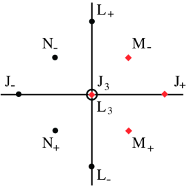
Figure 1: Root diagram for the $SO(1,4)$ group.

The roots are the various generators, displayed according to their weight, measured by their commutator with the two Cartan generators $J_{3}=(T^{12}+T^{34})$ and $L_{3}=(T^{12}-T^{34})$. The other compact generators are $J_{\pm}$ and $L_{\pm}$, which complete the $SU(2)\times SU(2)\simeq SO(4)$ stability group. The non–compact generators (boosts) are $M_{\pm}$ and $N_{\pm}$.

In these conventions, the $T_{orb}$ generator is given by either $e^{\frac{2\pi{\rm i}}{n}J_{3}}$ or $e^{\frac{2\pi{\rm i}}{n}L_{3}}$ and therefore the elements commuting with it are all the generators on the line orthogonal to the $(1,0)$ or $(0,1)$ vector in the root space. This implies that the remaining group generators are the sets $\{J_{\pm},J_{3},L_{3}\}$ or $\{L_{\pm},J_{3},L_{3}\}$ which span $SU(2)\times U(1)$. On the other hand, if we now look at the $\kappa=-1$ case, the generator which defines the surviving isometry group can be chosen to be $e^{\frac{2\pi{\rm i}}{n}(J_{3}\pm L_{3})}$. The residual symmetry group is then generated by the elements commuting with it and these are all the generators on the line orthogonal to the $(1,\pm 1)$ vector. The resulting set will be then given by $\{N_{-},M_{+},J_{3}\pm L_{3}\}$ or $\{N_{+},M_{-},J_{3}\pm L_{3}\}$, both generating $SL(2,{\mathbb{R}})\times U(1)$. As already remarked, the case $\kappa=0$ cannot be obtained in this same way. One can anyway see that the correct commutation relations are obtained by any solvable sub-algebra of the $so(1,4)$ one which sits on one of the corners of the diagram. One example is given by the red diamond generators in Figure (1), namely $\{J_{3},L_{3},J_{+},M_{\pm}\}$.

The ${\mathbb{E}}AdS_{4}$ space is a symmetric quaternionic space and therefore the analysis of the supersymmetric vacua obtained by gauging its isometries easily follows from the considerations made in [17]. Indeed it has been shown that if one looks only at the theory of supergravity coupled with hypermultiplets, the isometries leading to critical points are identified as those lying in the stability subgroup of the isometry group. The result is that one can obtain supersymmetric critical points of the potential by gauging isometries in $SO(4)$.

We have just seen that the isometries of our non–homogeneous quaternionic spaces can be understood as subsets of those of such ${\mathbb{E}}AdS_{4}$ space and it can also be shown that in the limit which gives back such space $n\to 0$, the isometries can indeed be identified. As a consequence, one could expect that the possibility of obtaining supersymmetric vacua from the gauging of the (59) isometries depends on such identification. For instance, from the above analysis, a critical point should follow from the gauging of any isometry in the $\kappa=1$ case, but only for special combinations in the $\kappa=-1$ and $\kappa=0$ cases.

5 Critical points and a domain wall solution

As next step we will give all critical points that can be obtained by the gauging described before. We will start with some general remarks followed by a detailed analysis of the critical points for the given model. A novel feature of this model is that it allows for multiple critical points such that we can construct a smooth domain wall solution interpolating between them.

5.1 Characterizing critical points

For a given superpotential it is a non-trivial question to determine all critical points, but in gauged supergravity, critical points can be directly determined from the Killing vectors [27, 31, 39, 17]. In our case, where only a single isometry has been gauged the situation is especially clear.

A direct consequence of the flow equations, is that the supersymmetric flow goes perpendicular to the Killing vector $k$ and hence terminates at points where $k$ becomes null, i.e. $|k|^{2}=0$. This fixed point set spans an even-dimensional submanifold. To see this one considers a parallel transport of the Killing vector $k$ along a vector $l$ so that $\delta k_{{\hbox{\tiny$X$}}}\sim(\nabla_{{\hbox{\tiny$Y$}}}k_{{\hbox{\tiny$X$}}})l^{{\hbox{\tiny$Y$}}}=(\partial_{[{\hbox{\tiny$Y$}}}k_{{\hbox{\tiny$X$}}]})l^{{}^{Y}}$; where we assumed a regular coordinate system and used the Killing property. Hence, if $dk\neq 0$ the number of possible translations along the null hypersurface is given by the rank of the 2-form $dk$ calculated on the null surface. If there are no non-trivial translations, the null hypersurface is just a point of the manifold, a so-called nut. If the rank is two implies that there are two translations that leave the null hypersurface and the other two stay inside. Hence the corresponding fixed point set is a 2-dimensional surface or a so-called bolt, see [51] for more details. In both cases one can construct a flow that terminates at the fixed point where $|k|^{2}=0$. In the degenerate case however, i.e. if $(\nabla_{{\hbox{\tiny$X$}}}k_{{\hbox{\tiny$Y$}}})(\nabla^{{\hbox{\tiny$X$}}}k^{{\hbox{\tiny$Y$}}})=0$, the flow can never reach the null hypersurface. To see this note that in the degenerate case the Killing vector and all derivatives vanish on the hypersurface; recall any Killing vector obeys the relation $\nabla_{{\hbox{\tiny$X$}}}\nabla_{{\hbox{\tiny$Y$}}}k_{{\hbox{\tiny$Z$}}}=R_{{\hbox{\tiny$Z$}}{\hbox{\tiny$Y$}}{\hbox{\tiny$X$}}{\hbox{\tiny$W$}}}k^{{\hbox{\tiny$W$}}}$. The Killing vector is therefore non–analytic and there is no possible perturbative expansion around such a point. Since the Killing vector is non-trivial in the interior we infer that a flow can never reach this point and exhibits a run-away behavior. In addition, in the degenerate case the surface gravity vanishes, whereas for the non-degenerate case not. As it is known from black holes, a non-vanishing surface gravity implies a periodicity of the coordinate along the Killing direction, whereas in the degenerate case this coordinate is non-compact. This is in agreement with the situation for homogeneous spaces where a gauging of a compact direction yields a fixed point, which may result in a flat or anti-deSitter spacetime whereas the gauging of a non-compact directions produces a run-away solution [17]. Let us add a further side remark. Especially in the case of a 4-dimensional quaternionic space, one can express the superpotential only by the discussed 2-form $dk=\partial_{{\hbox{\tiny$X$}}}k_{{\hbox{\tiny$Y$}}}dq^{{\hbox{\tiny$X$}}}\wedge dq^{{}^{Y}}$. Namely, for flat tangent space indices we can use the relation for our complex structures

$$\sum_{r}J^{r}_{{\hbox{\tiny$X$}}{\hbox{\tiny$Y$}}}J^{r}_{{\hbox{\tiny$Z$}}{\hbox{\tiny$W$}}}=-\epsilon_{{\hbox{\tiny$X$}}{\hbox{\tiny$Y$}}{\hbox{\tiny$Z$}}{\hbox{\tiny$W$}}}+\big{(}\delta_{{\hbox{\tiny$X$}}{\hbox{\tiny$Z$}}}\delta_{{\hbox{\tiny$Y$}}{\hbox{\tiny$W$}}}-\delta_{{\hbox{\tiny$X$}}{\hbox{\tiny$W$}}}\delta_{{\hbox{\tiny$Y$}}{\hbox{\tiny$Z$}}}\big{)}$$ (70)

and write with (17) and (15) for the superpotential

$$W^{2}={1\over 3}\Big{(}dk\wedge{{}^{\star}dk}-{1\over 2}dk\wedge dk\Big{)}\ .$$ (71)

For higher dimensional quaternionic spaces an analogous relation holds, which however includes curvature terms.

In summary, good critical points resulting in vacua with fixed or constant scalars, are given if the following relations are satisfied

$$|k|^{2}=g_{{\hbox{\tiny$X$}}{\hbox{\tiny$Y$}}}k^{{\hbox{\tiny$X$}}}k^{{\hbox{\tiny$Y$}}}=0\quad,\quad(\nabla_{{\hbox{\tiny$X$}}}k_{{\hbox{\tiny$Y$}}})(\nabla^{{\hbox{\tiny$X$}}}k^{{\hbox{\tiny$Y$}}})\neq 0\quad,\quad R_{{\hbox{\tiny$X$}}{\hbox{\tiny$Y$}}{\hbox{\tiny$Z$}}{\hbox{\tiny$W$}}}R^{{\hbox{\tiny$X$}}{\hbox{\tiny$Y$}}{\hbox{\tiny$Z$}}{\hbox{\tiny$W$}}}\neq\infty\ .$$ (72)

These relations are independent of the choosen coordinate system, but of course at these points one can always introduce a regular coordinate system and can infer that the Killing vector itself has to vanish [27, 39, 31, 17], which gives simpler equations. But note, in most cases there are no good global coordinates and it is better to use a coordinate independent notation.

For our model the situation is not so involved. The only delicate points in the metric are the zeros and the pole of $V$. The pole at $r=-n$, see eq. (32), represents a curvature singularity and we have to exclude this point. On the other hand the zeros of $V$ are regular points of the manifold and hence there is a regular coordinate system so that the metric is smooth there. As an example let us consider the Killing vector $k_{1}=\partial_{\tau}$. In this simple case $|k|^{2}=V=0$ at $r=r_{\pm},n$. At $r=r_{\pm}$ the fixed point set represents a bolt, because the 2-d base space $d\Sigma_{\kappa}$ remains finite, see (22), and at $r=n$ we have a nut, where the 2-d base space together with the $U(1)$ fiber vanishes. The surface gravity of the nut is given by $(\nabla_{{\hbox{\tiny$X$}}}k_{{\hbox{\tiny$Y$}}})(\nabla^{{\hbox{\tiny$X$}}}k^{{\hbox{\tiny$Y$}}})\sim{\kappa^{2}\over 4n^{2}}$ and hence for $\kappa=0$ the nut degenerates and is not a fixed point of the flow. The other fixed points at $r=r_{\pm}$ are always non-degenerate and the metric becomes regular if we introduce the coordinates

$$z={2\over\sqrt{\beta_{\pm}}}\sqrt{r-r_{{}_{\pm}}}\,e^{i\beta_{\pm}\tau}\ .$$ (73)

In fact as it clear from (57) the $(r,\tau)$-part of the metric becomes flat near the point $r=r_{\pm}$ and the Killing direction $\tau$ is compact. Moreover, after this transformation the new Killing vector becomes

$$k=\partial_{\tau}=\Big{(}{dz\over d\tau}\,\partial_{z}+{d\bar{z}\over d\tau}\,\partial_{\bar{z}}\Big{)}=i\beta_{\pm}\,(z\partial_{z}-\bar{z}\partial_{\bar{z}})$$ (74)

and the fixed point $r=r_{\pm}$ translates into $z=\bar{z}=0$, which is a zero of the new Killing vector.

5.2 Critical points

Let us now consider the isometry obtained by the generic linear combination

$$k=a^{I}k_{I}$$ (75)

and look for its zeroes.

The easiest case to analyze is $\kappa=0$. Critical points are obtained only if

$$a_{2}\neq 0\;\hbox{ and }\;a_{1}=4n\frac{a_{3}^{2}+a_{4}^{2}}{a_{2}}$$ (76)

and they lie at

$$x=-\frac{a_{3}}{a_{2}}\,,\quad y=\frac{a_{4}}{a_{2}}\,.$$ (77)

This means that for any value of the gauging parameter leading to critical points, this set is given by a plane in $r$ and $\tau$ for $x$ and $y$ fixed. No further critical points are obtained at $r=n$, as can be understood from the analysis of $k^{2}$ and $(\nabla k)^{2}$. The value of the cosmological constant at these critical points is given by

$${\cal V}=-\frac{a_{2}^{2}}{4}.$$ (78)

For $\kappa=1$, the analysis simplifies if one takes a different definition for the gauged isometry. Using the definition (65) of the $SU(2)\times U(1)$ generators given above, we can consider the critical points of the generic isometry defined by

$$k=\sum_{r=1}^{3}\alpha^{r}T_{r}+\beta T_{4}\ .$$ (79)

Let us now discuss first the case $r>n$ or $r<r_{-}$. In this case, the critical points appear (i.e. $k^{\hbox{\tiny$X$}}=0$) anytime

$$\beta=\mp 2n||\alpha||,$$ (80)

with $||\alpha||^{2}\equiv\sum_{r}\alpha_{r}^{2}$ being the $SU(2)$ norm of the parameters. They sit at

$$\begin{array}[]{lcr}x&=&\alpha_{1}\displaystyle\frac{\alpha_{3}\pm||\alpha||}{(\alpha_{1}^{2}+\alpha_{2}{}^{2})}\ ,\\ y&=&\displaystyle-\alpha_{2}\frac{\alpha_{3}\pm||\alpha||}{(\alpha_{1}^{2}+\alpha_{2}^{2})}\ .\end{array}$$ (81)

Of course the result should be the same for any direction inside the $SU(2)$ factor of the isometry and indeed, the limiting case $x=y=0$ for $\alpha_{1}=\alpha_{2}=0$ and $\beta=2n\alpha_{3}$ should also be included.

This set is given by a plane parameterized by $r$ and $\tau$ for any proper value of the gauging parameters. The interesting feature to note is that we cannot obtain critical points for any value of $\alpha_{r}$ and $\beta$, but we have to satisfy the constraint (80). This leads to a mismatch with the expectations coming from the previous group–theory analysis as we expected to have critical points for any value of the gauging parameters. This can be solved by considering the points at the boundaries of our space $r=n$ and $r=r_{-}$, which are the points where the metric (58) is not well behaved. Since we know that they are good points of the manifold, we should extend our analysis to these points. To do so one can compute the $|k|^{2}$ invariant and see whether at such points it vanishes. If we take $r=n$, this is indeed the case for any of the above isometries and $(\nabla k)^{2}$ is always different from zero at such point. This means that one always obtains at least one critical point for any gauging of the $SU(2)\times U(1)$ isometries, as expected. Moreover, in complete analogy with what happens for instance for the universal hypermultiplet [17], certain special combinations of two commuting $U(1)$’s make it degenerate to a full plane.

In the $r\geq n$ region we have then found an $SU(2)\times U(1)$ symmetric critical point (in some cases connected to a plane of critical points which preserve a $U(1)$). This reflects into the value of the cosmological constant at such critical points, which is

$${\cal V}=-\frac{||\alpha||^{2}}{4}$$ (82)

and shows the $SU(2)\times U(1)$ invariance explicitly. Again in complete analogy with the homogeneous case, the cosmological constant is generated by gauging the $SU(2)$ factor of the isometry, which will then be interpreted as the $R$–symmetry of the theory.

To complete such analysis we now have to consider the points at $r=r_{-}$ or $z=\bar{z}=0$ in the regular parameterization of (73). Here the result is somehow surprising and quite different from all the previous cases. Looking at the zeroes of $k^{2}$, which are not zeroes of $(\nabla k)^{2}$, one sees that two distinct critical points appear for any gauging of the $SU(2)\times U(1)$ isometries:

$$\begin{array}[]{rcl}r&=&r_{-}\equiv-n-\sqrt{4n^{2}-1}\,,\\[5.69054pt] x&=&x_{\pm}\equiv\alpha_{1}\displaystyle\frac{\alpha_{3}\pm||\alpha||}{(\alpha_{1}^{2}+\alpha_{2}{}^{2})}\,,\\[11.38109pt] y&=&y_{\pm}\equiv\displaystyle-\alpha_{2}\frac{\alpha_{3}\pm||\alpha||}{(\alpha_{1}^{2}+\alpha_{2}^{2})}\,.\end{array}$$ (83)

As for the point $r=n$ in the previous case we don’t need to impose (80). These critical points preserve a $U(1)\times U(1)$ symmetry which is generated by the following combinations of the Killing vectors

$$\begin{array}[]{rcl}k_{A}&=&\sqrt{4n^{2}-1}\,\alpha^{r}T_{r}+\beta\,T_{4}\\[5.69054pt] k_{B}&=&\sqrt{4n^{2}-1}\,\alpha^{r}T_{r}-\beta\,T_{4}\end{array}$$ (84)

This again shows up in the value of the cosmological constant at the critical points, which are given by

$${\cal V}_{x_{+},y_{+}}=-\frac{1}{4}(n-r_{-})^{2}A_{+}^{2}\ ,\quad\hbox{and}\quad{\cal V}_{x_{-},y_{-}}=-\frac{1}{4}(n-r_{-})^{2}A_{-}^{2}\ ,$$ (85)

for $A_{\pm}\equiv\beta\pm\sqrt{4n^{2}-1}||\alpha||$.

A comment is in order here. As pointed out in [22], for a large class of quaternionic–Kaḧler manifolds, critical points which are in the same branch of the moduli space must be connected through a geodesic line of critical points. It would be natural to expect the same to happen here. On the other hand we have shown above that these two critical points are isolated. The resolution of this apparent paradox is given by the fact that our space is not geodesically complete and that moreover the region containing the singularity is excluded from physical requirement. This implies that if we look for the points where the Killing vectors are vanishing in the whole space, we will see that indeed the above critical points are connected through a geodesic critical line, but that this latter lies completely inside the region of our moduli space which is not accessible. This results in two isolated points in the physical region, which are the boundaries of such geodesic. Moreover, as we will see in the next section, we are now allowed to find a supersymmetric flow interpolating between them. Actually, this flow is driven by the gradient of the superpotential and therefore does not necessarily follow geodesic lines.

In the case $\kappa=-1$ the $SO(2,1)$ norm

$$||\alpha||^{2}\equiv-\alpha_{1}^{2}-\alpha_{2}^{2}+\alpha_{3}^{2}$$ (86)

can be both positive or negative. If we analyze first the regions $r>r_{+}$ or $r<r_{-}$, we obtain critical points whenever $||\alpha||^{2}\geq 0$ and

$$\beta=\mp 2n||\alpha||\ .$$ (87)

The critical points sit at

$$\begin{array}[]{lcr}x&=&\alpha_{1}\displaystyle\frac{\alpha_{3}\pm||\alpha||}{(\alpha_{1}^{2}+\alpha_{2}{}^{2})}\,,\\ y&=&\displaystyle-\alpha_{2}\frac{\alpha_{3}\pm||\alpha||}{(\alpha_{1}^{2}+\alpha_{2}^{2})}\,,\end{array}$$ (88)

exactly matching the $\kappa=1$ case. This similarity extends to the value of the cosmological constant, which is given by

$${\cal V}=-\frac{||\alpha||^{2}}{4}\ .$$ (89)

If, on the other hand $||\alpha||^{2}<0$, critical points can only appear for $x^{2}+y^{2}=1$, which is out of the domain covered by our coordinate patch, cp. the metric in (58).

Extending the analysis to the points $r=r_{\pm}$, for each of the sections we find again two distinct critical points at $x=x_{\pm}$, $y=y_{\pm}$. Again they preserve a $U(1)\times U(1)$ symmetry generated by (84) and the cosmological constant evaluated at those points is given by ${\cal V}=-\frac{1}{4}(n-r_{\pm})^{2}A_{\pm}^{2}$. The fact that must be pointed out is that now these critical points lie in disconnected branches of our moduli space. One can indeed see that $x_{+}^{2}+y_{+}^{2}<1$, whereas $x_{-}^{2}+y_{-}^{2}>1$ and we can have at most one critical point for each connected region. This implies that we cannot build any regular flow interpolating between them.

5.3 A smooth domain wall solution

As we mentioned before our non-homogeneous space has two physical regions: $r\leq r_{-}$ and $r\geq{\rm max}\{n,r_{+}\}$. The situation in the latter case is very much similar to homogeneous spaces, which is expected since this range survives the limit giving ${\mathbb{E}}AdS_{4}$ or ${SU(2,1)\over U(2)}$. More interesting is the other physical region where $r\leq r_{-}$ and let us discuss an explicit example.

In the case that $\kappa=1$, we have seen that we can have two distinct critical points at $r=r_{-}$ (or equivalently $z=\bar{z}=0$ in the coordinates for which the metric is well behaved), $x=x_{\pm}$ and $y=y_{\pm}$. As we have seen in (85), the value of the potential, and therefore of the cosmological constant, at such points differs in general. This changes when the gauged symmetry is completely inside the $SU(2)$ factor of the isometry group or it is given by the extra $U(1)$. Let us therefore choose in the following the gauged isometry to be $k=4\sqrt{\frac{2}{3}}\,T_{1}$, where the coefficient has been fixed for later convenience. This implies that we will have two $AdS$ critical points with the same value of the cosmological constant in the same region of the moduli space, and that we can try to find the solution interpolating between them.

In the well behaved coordinates of (73), the Killing vector corresponding to this isometry is given by

$$k=\sqrt{\frac{8}{3}}\Big{[}\,{\rm i}\,4n\,x\,\beta_{\pm}(z\partial_{z}-\bar{z}\partial_{\bar{z}})+2\,xy\,\partial_{x}+(1-x^{2}+y^{2})\,\partial_{y}\Big{]}\ .$$ (90)

This gauging gives then two critical points at $x=\pm 1$, $y=0$ and $z=\bar{z}=0$. At both critical points the cosmological constant is ${\cal V}=-\frac{1}{4}(n-r_{-})^{2}(n+r_{+})^{2}$ and we are interested in the solution of the flow equations (20) interpolating between them. The corresponding superpotential $W$ can be obtained from the Killing prepotentials (60) using (17). For any value of $x$ one can also see that $\partial_{y}W(z,\bar{z},x,y)=\partial_{z}W(z,\bar{z},x,y)=\partial_{\bar{z}}W(z,\bar{z},x,y)=0$ if $z=\bar{z}=y=0$ and that therefore we can restrict to a flow in the single $x$ coordinate, keeping fixed the others. From (20) it follows indeed that in this case $y^{\prime}=z^{\prime}=\bar{z}^{\prime}=0$. The superpotential restricted to this line is only a function of $x$ and reads

$$W=\frac{4}{3}\;(n-r_{-})(n+r_{+})\;{x\over 1+x^{2}}$$ (91)

with $r_{\pm}=-n\pm\sqrt{4n^{2}-1}$.

Figure 2: On the left hand side we plotted the superpotential in the case $n=1$ as a function of $x$ and the right hand side the solution for the warp factor as function of $\rho$ interpolating between the two extrema

The flow equations for the scalar field $x$ and the warp factor $U$ become

$$\begin{array}[]{rcl}x^{\prime}&=&3\,g\,g^{xx}\partial_{x}W=\left(1-x^{2}\right)\,,\\[8.53581pt] U^{\prime}&=&-g\,W\,,\end{array}$$ (92)

whose solution is given by

$$ds^{2}=e^{2U}\,ds_{4d}+d\rho^{2}\quad,\qquad x=\tanh{(g\rho)}$$ (93)

with the warp factor

$$e^{2U}=\left[\cosh\left(2g\rho\right)\right]^{-\frac{1}{3}(n-r_{-})(n+r_{+})}\ .$$ (94)

The $AdS_{5}$ vacuum is reached at $\rho=\pm\infty$ and since $(n-r_{-})(n+r_{+})>0$ the warp factor vanishes exponentially on both sides of the wall, see also the rhs in picture (2). This means that this domain wall solution can trap gravity in the way suggested by Randall and Sundrum [6]. Moreover, as it can be seen from the picture (2), the superpotential shows two extrema at $x=\pm 1$ and our solution interpolates between them. As expected for brane–world type solutions, the superpotential $W$ crosses a point where it vanishes, which is related through (20) to the maximum of the warp factor. Note, that in the so-called thin-wall limit of large $g$ the scalar field becomes piecewise constant and the metric approaches $AdS_{5}$ for any non-vanishing value of $\rho$.

Our result could seem in contrast with the no–go theorem in [21], where the possibility of obtaining smooth Randall–Sundrum type solutions in some generic classes of supergravity theories is discussed. But one of the assumptions for their result to hold is that the potential should be non–positive ${\cal V}\leq 0$, at least in the range of values of scalar fields that is explored in the solution under consideration. This is not the case in our solution. Since the potential has a negative contribution coming from $W^{2}$ and a positive one coming from its derivatives, there are points along the solution where ${\cal V}>0$. Take for instance the point $x=0$, where $W=0$. At that point $\partial_{x}W\neq 0$ (as the flows does not stop there) and therefore the potential has a positive value. This means that our example cannot be included into the class of solutions considered in [21] and therefore avoids the no–go theorem presented there.

6 Conclusion

We discussed a class of 4–dimensional non–homogeneous quaternionic spaces, which admit four isometries and have two disconnected physical regions, where the metric is regular and positive definite. Between these two regions the space has timelike directions and exhibits a curvature singularity. This space is constructed as a non–trivial line bundle over a 2–d base space of constant curvature $\kappa$. For $\kappa=1$, this quaternionic space is the AdS-Taub-NUT solution with a special value of the mass parameter and represents a resolution of an orbifold of the Euclidean $AdS_{4}$ space. For vanishing NUT charge the space becomes $AdS_{4}$ and in the limit of infinite NUT charge it becomes ${SU(2,1)\over SU(2)\times U(1)}$. Therefore, it can be seen as an interpolating solution between the two known homogeneous 4-d quaternionic spaces.

As long as one considers the physical parameter range, where the metric is positive definite, this space can be regarded in $N=2$ gauged supergravity as the space parameterized by one hypermultiplet. Doing this, we discussed in the second part of the paper the isometries, their gauging and the critical points of the resulting potential. We found for $\kappa=1$ that the critical points differ significantly in the two allowed regions. In one region the situation is very much similar to the gauging of the homogeneous spaces, i.e. there are no multiple critical points (or critical surfaces) and hence there are no smooth domain wall solutions. In the other region however, we found two critical points with different values of the cosmological constant, that are located exactly on the boundary of the physical parameter range. The value of cosmological constant as well as the nature of the critical points can continuously be changed while varying the gauging parameters. For a specific gauging we constructed explicitly a smooth domain wall solution. Since this solution interpolates between two IR critical points, the warp factor is exponentially suppressed on both sides and thus gravity can be trapped near this wall.

There are number of directions, which are worthwhile to pursue. We considered only an Abelian gauging of this space, but one may also consider non-Abelian gaugings or discuss the gauging of two Abelian isometries. In both cases one would have to couple this model also to vector multiplets. This should be a straightforward generalization, but more interesting would be to ask whether this space can appear in compactified string- or M-theory and if yes, can one understand the smooth domain wall in terms of branes. Finally, it is needless to say, that it would be interesting to construct also other non-homogeneous quaternionic spaces and to discuss the resulting vacuum structure (as e.g. the spaces discussed in [33]).

Acknowledgments

We would like to thank Antoine van Proeyen for helpful discussions. The work of K.B. is supported by a Heisenberg grant of the DFG and G. D. acknowledges the financial support provided through the European Community’s Human Potential Programme under contract HPRN-CT-2000-00131 quantum spacetime.

References

- [1] E. Alvarez and C. Gomez, “Geometric holography, the renormalization group and the c- theorem,” Nucl. Phys. B541 (1999) 441–460, http://arXiv.org/abs/hep-th/9807226.
- [2] D. Z. Freedman, S. S. Gubser, K. Pilch, and N. P. Warner, “Renormalization group flows from holography supersymmetry and a c-theorem,” Adv. Theor. Math. Phys. 3 (1999) 363–417, http://arXiv.org/abs/hep-th/9904017.
- [3] L. Girardello, M. Petrini, M. Porrati, and A. Zaffaroni, “Novel local CFT and exact results on perturbations of N = 4 super Yang-Mills from AdS dynamics,” JHEP 12 (1998) 022, http://arXiv.org/abs/hep-th/9810126.
- [4] K. Akama, “An early proposal of ’brane world’,” Lect. Notes Phys. 176 (1982) 267–271, http://arXiv.org/abs/hep-th/0001113.
- [5] V. A. Rubakov and M. E. Shaposhnikov, “Do we live inside a domain wall?,” Phys. Lett. B125 (1983) 136–138.
- [6] L. Randall and R. Sundrum, “An alternative to compactification,” Phys. Rev. Lett. 83 (1999) 4690–4693, http://arXiv.org/abs/hep-th/9906064.
- [7] A. Lukas, B. A. Ovrut, K. S. Stelle, and D. Waldram, “The universe as a domain wall,” Phys. Rev. D59 (1999) 086001, http://arXiv.org/abs/hep-th/9803235.
- [8] R. Altendorfer, J. Bagger, and D. Nemeschansky, “Supersymmetric Randall-Sundrum scenario,” Phys. Rev. D63 (2001) 125025, http://arXiv.org/abs/hep-th/0003117.
- [9] E. Bergshoeff, R. Kallosh, and A. Van Proeyen, “Supersymmetry of RS bulk and brane,” Fortsch. Phys. 49 (2001) 625–632, http://arXiv.org/abs/hep-th/0012110.
- [10] E. Bergshoeff, R. Kallosh, and A. Van Proeyen, “Supersymmetry in singular spaces,” JHEP 10 (2000) 033, http://arXiv.org/abs/hep-th/0007044.
- [11] K. Behrndt and S. Gukov, “Domain walls and superpotentials from M-theory on Calabi-Yau three-folds,” Nucl. Phys. B580 (2000) 225–242, http://arXiv.org/abs/hep-th/0001082.
- [12] G. Curio, A. Klemm, D. Lüst, and S. Theisen, “On the vacuum structure of type II string compactifications on Calabi-Yau spaces with H-fluxes,” Nucl. Phys. B609 (2001) 3–45, http://arXiv.org/abs/hep-th/0012213.
- [13] G. Dall’Agata, “Type IIB supergravity compactified on a Calabi-Yau manifold with H-fluxes,” JHEP 11 (2001) 005, http://arXiv.org/abs/hep-th/0107264.
- [14] R. Kallosh and A. D. Linde, “Supersymmetry and the brane world,” JHEP 02 (2000) 005, http://arXiv.org/abs/hep-th/0001071.
- [15] K. Behrndt and M. Cvetic, “Anti-de Sitter vacua of gauged supergravities with 8 supercharges,” Phys. Rev. D61 (2000) 101901, http://arXiv.org/abs/hep-th/0001159.
- [16] K. Behrndt, “Domain walls and flow equations in supergravity,” Fortsch. Phys. 49 (2001) 327–338, http://arXiv.org/abs/hep-th/0101212.
- [17] A. Ceresole, G. Dall’Agata, R. Kallosh, and A. Van Proeyen, “Hypermultiplets, domain walls and supersymmetric attractors,” Phys. Rev. D64 (2001) 104006, arXiv:hep-th/0104056.
- [18] M. Cvetic, S. Griffies, and S.-J. Rey, “Static domain walls in N=1 supergravity,” Nucl. Phys. B381 (1992) 301–328, http://arXiv.org/abs/hep-th/9201007.
- [19] G. W. Gibbons and N. D. Lambert, “Domain walls and solitons in odd dimensions,” Phys. Lett. B488 (2000) 90–96, http://arXiv.org/abs/hep-th/0003197.
- [20] A. Ceresole and G. Dall’Agata, “Brane-worlds in 5D supergravity,” Fortsch. Phys. 49 (2001) 449–454, http://arXiv.org/abs/hep-th/0101214.
- [21] J. Maldacena and C. Nunez, “Supergravity description of field theories on curved manifolds and a no go theorem,” Int. J. Mod. Phys. A16 (2001) 822–855, http://arXiv.org/abs/hep-th/0007018.
- [22] D. V. Alekseevsky, V. Cortes, C. Devchand, and A. Van Proeyen, “Flows on quaternionic-kaehler and very special real manifolds,” http://arXiv.org/abs/hep-th/0109094.
- [23] M. Gunaydin, G. Sierra, and P. K. Townsend, “Gauging the d = 5 Maxwell-Einstein supergravity theories: More on Jordan algebras,” Nucl. Phys. B253 (1985) 573.
- [24] M. Gunaydin and M. Zagermann, “The vacua of 5d, N=2 gauged Yang-Mills/Einstein/tensor supergravity: Abelian case,” Phys. Rev. D62 (2000) 044028, http://arXiv.org/abs/hep-th/0002228.
- [25] M. Gunaydin and M. Zagermann, “The gauging of five-dimensional, N=2 Maxwell-Einstein supergravity theories coupled to tensor multiplets,” Nucl. Phys. B572 (2000) 131–150, http://arXiv.org/abs/hep-th/9912027.
- [26] J. Bagger and E. Witten, “Matter couplings in N=2 supergravity,” Nucl. Phys. B222 (1983) 1.
- [27] A. Ceresole and G. Dall’Agata, “General matter coupled N = 2, D = 5 gauged supergravity,” Nucl. Phys. B585 (2000) 143–170, arXiv:hep-th/0004111.
- [28] K. Behrndt, C. Herrmann, J. Louis, and S. Thomas, “Domain walls in five dimensional supergravity with non- trivial hypermultiplets,” JHEP 01 (2001) 011, http://arXiv.org/abs/hep-th/0008112.
- [29] K. Behrndt and M. Cvetic, “Gauging of N = 2 supergravity hypermultiplet and novel renormalization group flows,” Nucl. Phys. B609 (2001) 183–192, http://arXiv.org/abs/hep-th/0101007.
- [30] M. Cvetic, H. Lu, and C. N. Pope, “Localized gravity in the singular domain wall background?,” http://arXiv.org/abs/hep-th/0002054.
- [31] K. Behrndt, S. Gukov, and M. Shmakova, “Domain walls, black holes, and supersymmetric quantum mechanics,” Nucl. Phys. B601 (2001) 49–76, http://arXiv.org/abs/hep-th/0101119.
- [32] E. Ivanov and G. Valent, “Quaternionic Taub-NUT from the harmonic space approach,” Phys. Lett. B 445, 60 (1998) [arXiv:hep-th/9809108].
- [33] P. Y. Casteill, E. Ivanov and G. Valent, “Quaternionic extension of the double Taub-NUT metric,” Phys. Lett. B 508, 354 (2001) [arXiv:hep-th/0104078].
- [34] J. Wolf, “Complex homogenous contact manifolds and quaternionic symmetric spaces,” J. Math. Mech. 14 (1965) 1033.
- [35] D. Alekseevsky, “Classification of quaternionic spaces with a transitive solvable group of motions,” Math USSR Izv. 9 (1975) 297.
- [36] K. Becker, M. Becker, and A. Strominger, “Five-branes, membranes and nonperturbative string theory,” Nucl. Phys. B456 (1995) 130–152, http://arXiv.org/abs/hep-th/9507158.
- [37] A. Strominger, “Loop corrections to the universal hypermultiplet,” Phys. Lett. B421 (1998) 139–148, http://arXiv.org/abs/hep-th/9706195.
- [38] S. V. Ketov, “Quantum geometry of the universal hypermultiplet,” arXiv:hep-th/0111080.
- [39] R. D’Auria and S. Ferrara, “On fermion masses, gradient flows and potential in supersymmetric theories,” JHEP 05 (2001) 034, http://arXiv.org/abs/hep-th/0103153.
- [40] D. Kramer, E. Herlt, M. MacCallum, and H. Stephani, “Exact solutions of Einstein’s field equations,” Cambridge University Press (1979).
- [41] K. Galicki, “A generalization of the momentum mapping construction for quaternionic kahler manifolds,” Commun. Math. Phys. 108 (1987) 117.
- [42] R. D’Auria, S. Ferrara, and P. Fre, “Special and quaternionic isometries: General couplings in n=2 supergravity and the scalar potential,” Nucl. Phys. B359 (1991) 705–740.
- [43] L. Andrianopoli et. al., “N = 2 supergravity and N=2 super Yang-Mills theory on general scalar manifolds: Symplectic covariance, gaugings and the momentum map,” J. Geom. Phys. 23 (1997) 111–189, hep-th/9605032.
- [44] D. N. Page and C. N. Pope, “Inhomogeneous Einstein metrics on complex line bundles,” Class. Quant. Grav. 4 (1987) 213.
- [45] A. Chamblin, R. Emparan, C. V. Johnson, and R. C. Myers, “Large N phases, gravitational instantons and the Nuts and Bolts of AdS holography,” Phys. Rev. D59 (1999) 064010, hep-th/9808177.
- [46] S. Ferrara and S. Sabharwal, “Quaternionic manifolds for type II superstring vacua of Calabi-Yau spaces,” Nucl. Phys. B332 (1990) 317.
- [47] R. B. Mann, “Topological black holes: Outside looking in,” gr-qc/9709039.
- [48] M. Banados, A. Gomberoff, and C. Martinez, “Anti-de Sitter space and black holes,” Class. Quant. Grav. 15 (1998) 3575–3598, http://arXiv.org/abs/hep-th/9805087.
- [49] K. Behrndt and D. Lüst, “Branes, waves and AdS orbifolds,” JHEP 07 (1999) 019, http://arXiv.org/abs/hep-th/9905180.
- [50] G. W. Gibbons and S. W. Hawking, “Gravitational multi - instantons,” Phys. Lett. B78 (1978) 430.
- [51] G. W. Gibbons and S. W. Hawking, “Classification of gravitational instanton symmetries,” Commun. Math. Phys. 66 (1979) 291.