Noncommutative quantum mechanics in the presence of delta-function potentials

Abstract

Quantum mechanics in the presence of $\delta$-function potentials is known to be plagued by UV divergencies which result from the singular nature of the potentials in question. The standard method for dealing with these divergencies is by constructing self-adjoint extensions of the corresponding Hamiltonians. Two particularly interesting examples of this kind are nonrelativistic spin zero particles in $\delta$-function potential and Dirac particles in Aharonov-Bohm magnetic background. In this paper we show that by extending the corresponding Schrödinger and Dirac equations onto the flat noncommutative space a well-defined quantum theory can be obtained. Using a star product and Fock space formalisms we construct the complete sets of eigenfunctions and eigenvalues in both cases which turn out to be finite.

I Introduction

Singular interaction potentials were introduced in quantum mechanics more than sixty years ago old . Since then they found applications in various areas of solid state condensed , particle particle and nuclear nuclear physics. It has also been known for a long time that local nature of these potentials at all scales leads to appearance ultraviolet divergencies in quantum mechanics similar to those encountered in quantum field theory. However, unlike quantum field theory in which one meets UV divergensies primarilly due to the presence of infinite number of degrees of freedom, in quantum mechanics the infinities occur due to the singular nature of the potentials chosen. Mathematical theory of how to treat such potentials is well known Reed , Alberverio and is based on construction of self-adjoint extensions of the Hamiltonians in question.

On the other hand there has been a lot of recent interest in noncommutative spaces Madore , Connes , Konechny motivated primarilly by string string and field theory field applications. In particular, on the field theory side it is believed that in certain cases noncommutative modification of the algebraic structure of space-time can provide a natural regularization of UV divergencies. This is certainly the case for compact manifolds Grosse1 , Grosse since field theories on the noncommutative generalizations of such manifolds posess only finite number of degrees of freedom thus removing the intrinsic reason for appearance of UV divergencies.

The purpose of the present paper is to study the quantum mechanics on the flat noncommutative two dimensional space Nair in the presence of singular potentials and to show that nonlocality of interaction induced by fuzziness of space leads to a well-defined quantum theory. In Section II we consider nonrelativistic spin zero particles in a $\delta$-function potential and after a brief discussion of the main results known from the commutative case Jackiw , Perry we give a complete analytic solution of the corresponding Schrödinger equation over the noncommutative plane. Section III deals with spin-$\frac{1}{2}$ relativistic particles in the Aharonov-Bohm background magnetic field and we use Fock space formalism to obtain the complete set of eigenfunctions for this problem. Also the relationship between commutative and noncommutative solutions is discussed and we show that in the limit of vanishing noncommutativity parameter $\theta$ we recover the same solutions as those given by theory of self-adjoint extensions.

Our notations and conventions as well as a review of star-product and Fock space formalisms in noncommutative geometry are given in Appendix.

II Two-Dimensional Delta-function Potential.

II.1 Commutative case.

In the commutative case the Schrödinger equation for spin zero particle moving in a two-dimensional $\delta$-function potential, can be written as ($\hbar=1$)

$$-\frac{1}{2m}\nabla^{2}\Psi({\bf r})+V_{0}\delta({\bf r})\Psi({\bf r})=E\Psi({\bf r})$$ (1)

or, in terms of new coupling constant $\alpha_{0}=2mV_{0}$ and energy parameter $\tilde{E}=2mE$,

$$-\nabla^{2}\Psi({\bf r})+\alpha_{0}\delta({\bf r})\Psi({\bf r})=\tilde{E}\Psi({\bf r}).$$ (2)

Both the $\delta$-function potential in two dimensions and the kinetic energy operator scale in polar coordinates $(\rho,\phi)$ as $1/\rho^{2}$, therefore the coupling $\alpha_{0}$ is dimensionless. As a consequence, the Hamiltonian is scale invariant and we can anticipate the presence of logarithmic ultraviolet divergencies, analogous to those appearing in QED and QCD. The standard way of obtaining an exact solution of (2) analytically is to use method of self-adjoint extensions. As explained in Jackiw , the two-dimensional Laplace operator $\nabla^{2}$ is not self-adjoint on a punctured plane and construction of self-adjoint extension requires relaxing the condition of regularity of wave functions at the origin and allowing $\log\rho$ singularity at $\rho=0$. However, $\delta(\rho)\log\rho$ is then not well-defined. Thus, we need to define $\delta(\rho)\Psi(\rho,\phi)$ for wavefunctions behaving near the origin as

$$\Psi(\rho,\phi)=\psi_{0}\log(\mu\rho)+\psi_{1}+O(\rho).$$ (3)

where $\mu$ is an arbitrary dimensional parameter. Formal integration of eq.(2) over a small disk of radius $\epsilon$ followed by taking the limit $\epsilon\to 0$ gives the correct constraint on coefficients $\psi_{0}$ and $\psi_{1}$

$$2\pi\psi_{0}-\alpha_{0}\psi_{1}=0$$ (4)

which we should take as a boundary condition on a wavefunction. More detailed derivation of (4) can be found in Reed .

With these ideas in mind we can rewrite (2) for an axially symmetric wavefunction as

$$\Psi^{\prime\prime}(\rho)+\frac{1}{\rho}\Psi^{\prime}(\rho)+\tilde{E}\Psi(\rho)=0$$ (5)

which for $\tilde{E}<0$ admits

$$\Psi(\rho)=K_{0}\left(\sqrt{|\tilde{E}|}\ \rho\right)$$ (6)

as a solution. Here $K_{0}(x)$ is the modified Bessel function of the third kind Bateman . From the asymptotic behaviour of $\Psi(\rho)$ near the origin, namely,

$$\Psi(\rho)=-\log\left(\frac{\tilde{E}\rho}{2}\right)-\gamma+O(\rho)$$ (7)

and the boundary condition (4) we find an expression for the energy of this bound state

$$\tilde{E}=-4\mu^{2}e^{-2\gamma}e^{\frac{4\pi}{\alpha_{0}}}.$$ (8)

Therefore this theory provides us with an example of a spontaneous breakedown of scale invariance where bound state energy is set by an arbitrary dimensionful parameter $\mu$.

II.2 Noncommutative case

In complete analogy with commutative case we can write the Schrödinger equation for a particle moving in a noncommutative $\delta$-function potential as

$$-\hat{\nabla}^{2}\hat{\Psi}({\bf\hat{x}})+\alpha_{0}\hat{\delta}(\hat{x})\hat{\Psi}({\bf\hat{x}})=\tilde{E}\hat{\Psi}({\bf\hat{x}}),$$ (9)

but where $\hat{\Psi}({\bf\hat{x}})$ now is an operator valued wavefunction

$$\hat{\Psi}({\bf\hat{x}})=\int d^{2}p\ \Phi(p,\bar{p})e^{i(pz+\bar{p}\bar{z})}$$

and $\hat{\delta}(\hat{x})$ is defined in (68).

In momentum space equation (9) becomes

$$(p\bar{p}-\tilde{E})\Phi(p,\bar{p})=-\frac{\alpha_{0}}{(2\pi)^{2}}\int d^{2}\eta\ \Phi(\eta,\bar{\eta})\ e^{-\frac{\theta}{4}|p-\eta|^{2}+\frac{\theta}{4}(\bar{p}\eta-p\bar{\eta})}$$ (10)

with parameters $\tilde{E}=2mE$ and $\alpha_{0}=2mV_{0}$ defined as in commutative case.

Equation (10) is an integral equation for momentum space wave-function which, in general, is difficult to solve. But the solution of this particular equation is greatly simplified if one observes that the differential operator

$$\frac{\partial}{\partial p}+\frac{\theta}{4}\bar{p}$$ (11)

when applied to the r.h.s of (10) gives zero, and, therefore, we are left only with

$$\left[\frac{\partial}{\partial p}+\frac{\theta}{4}\bar{p}\right](|p|^{2}-\tilde{E})\Phi(p,\bar{p})=0$$ (12)

This last equation is easy to solve and, after we pass to the eigenstates $\Phi_{n}(p)$ of angular momentum operator

$$\Phi(p,\phi)=\sum_{n=-\infty}^{\infty}\ \Phi_{n}(p)e^{in\phi},$$ (13)

its solutions are given by

$$\Phi_{n}(p)=\frac{p^{n}}{p^{2}-\tilde{E}}\ e^{-\frac{\theta}{4}p^{2}},\ \ \ \ n=0,\pm 1,\pm 2,\ldots\$$ (14)

for $\tilde{E}<0$, while for positive energies eq.(12) admits an extra $\delta$-function term and therefore we write

$$\Phi_{n}(p)=\delta(p^{2}-\tilde{E})+C_{n}\frac{p^{n}}{p^{2}-\tilde{E}}\ e^{-\frac{\theta}{4}p^{2}}$$ (15)

By direct substitution, it can be verified that eq.(15) gives a complete set of scattering states provided that constants $C_{n}$ are choosen as the solutions of

$$1=-\frac{\alpha_{0}}{4\pi}\left\{C_{n}I_{n}\left(\frac{\theta\tilde{E}_{n}}{2}\right)+{1\over{n!}}\ e^{-{\theta\over{4}}\tilde{E}}\left({\theta\over{2}}\sqrt{\tilde{E}}\right)^{n}\right\}$$ (16)

for $n\geq 0$, and $C_{n}=0$ for $n<0$, with functions $I_{n}$ defined by

$$I_{n}(a)={1\over{n!}}\int_{0}^{\infty}dt\frac{t^{n}}{t-a}e^{-t}=(-a)^{n}\Psi(n+1,n+1,-a)$$

and where $\Psi(a,b,c)$ is the confluent hypergeometric function.

Similar analysis shows that Eqs.14 also satisfy Schrödinger equation for $n\geq 0$ only, thus giving us bound state solutions the number of which, as well as their energies being given by the following set of eigenvalue equations

$$1=-\frac{\alpha_{0}}{4\pi}\ I_{n}\left(-\frac{\theta|\tilde{E}_{n}|}{2}\right).$$ (17)

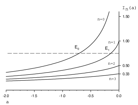
Figure 1: Example of graphical solution of eigenvalue equation (14). In this case we have two bound states.

Example of a graphical solution of these equations is presented in Fig.1, from which it can also be seen, that like in commutative case, the radially symmetric solution ($n=0$) exists for arbitrary strength of attractive potential but, unlike the commutative case, for sufficiently strong potentials (when dimensionless coupling $|\alpha_{0}|>1$) this problem also admits bound states with nonzero angular momentum ($n>0$), the number of such solutions being a function of $\alpha_{0}$ only. It is also instructive to look at limiting cases of very strong and very weak binding potential more closely.

II.2.1 Large coupling ($|\alpha|\gg 1$)

In this case $a=\frac{\theta|\tilde{E}|}{2}\gg 1$ and we can use asymptotic expansion

$$I_{n}(a)={1\over a}-{\frac{n+1}{a^{2}}}+O\left({1\over{a^{3}}}\right)$$

and write (14) as

$$1=\frac{|\alpha_{0}|}{4\pi}\left({1\over{a_{n}}}-{\frac{n+1}{a_{2}^{2}}}\right)$$

with solutions

$$a_{n}=\frac{4\pi}{|\alpha_{0}|}-(n+1)$$

or

$$\tilde{E}_{n}=-\frac{2}{\theta}a_{n}=\frac{8\pi}{\theta\alpha_{0}}+\frac{2}{\theta}(n+1)$$

and we see that bound state spectrum in this case coincides with that of a simple harmonic ocsillator of frequency $\frac{2}{\theta}$ Gamboa .

II.2.2 Small coupling ($|\alpha|\ll 1$)

In this case only one solution of (17) exists corresponding to $n=0$ and $a=\frac{\theta|\tilde{E}|}{2}\ll 1$. Therefore, we can use the asymptotic form of $I_{n}(a)$ for small $a$’s which is

$$I_{0}(a)=-\ln|a|-\gamma+O(|a|\ln|a|)$$ (18)

$$\gamma=0.5772\ldots\ ,\ \mbox{Euler's constant}$$ (19)

This gives the following eigenvalue equation

$$1=\frac{|\alpha_{0}|}{4\pi}(\ln|a|+\gamma)$$

with binding energy

$$|\tilde{E}|=\frac{2}{\theta}e^{-\gamma}e^{\frac{4\pi}{\alpha_{0}}}$$

Comparing this last expression with (8) we see that this limit corresponds to the commutative case with $1\over\theta$ playing the rôle of parameter $\mu^{2}$ in commutative case.

III Fermions in a magnetic vortex background

III.1 Commutative case

In this section we briefly review the solutions of a massive Dirac equation in the Aharonov-Bohm background field of an infinitely thin magnetic vortex carrying magnetic flux $\Phi$. This presentation closely follows Ref.Gerbert . The electromagnetic potential describing such field configuration can be chosen in polar coordinates $(\rho,\phi)$ as ${\mathbf{A}}=-\frac{e\Phi}{2\pi}\frac{1}{\rho}{\mathbf{\hat{\phi}}}$. $\mathbf{A}$ has a well known property of being locally a pure gauge.

The Dirac equation for this problem is

$$(i\not{\!\partial}+\not{\!\!A}-m)\Psi(t,r,\phi)=0.$$ (20)

and allows passing to the eigenstates of angular momentum $n+\frac{1}{2}$. By defining

$$\Psi_{E,n}(t,\rho,\phi)=\left(\begin{array}[]{c}\chi^{1}(\rho)e^{in\phi}\\ \chi^{2}(\rho)e^{i(n+1)\phi}\end{array}\right)e^{-iEt}$$ (21)

the radial eigenvalue problem is

$$\left(\begin{array}[]{cc}m-E&-i\left(\partial_{\rho}+\frac{\nu+1}{\rho}\right)\\ -i\left(\partial_{\rho}-\frac{\nu}{\rho}\right)&-m-E\end{array}\right)\chi(\rho)=0$$ (22)

with $\nu\equiv n+\Phi$. For $E^{2}>m^{2}$ it has the solutions

$$\chi_{\nu}(\rho)=\frac{1}{N}\left(\begin{array}[]{c}\sqrt{E+m}(\epsilon_{n})^{n}J_{\epsilon_{n}\nu}(k\rho)\\ i\sqrt{E-m}(\epsilon_{n})^{n+1}J_{\epsilon_{n}(\nu+1)}(k\rho)\end{array}\right)$$ (23)

where $N$ is a normalization factor, $k=\sqrt{E^{2}-m^{2}}$, $J_{\lambda}(x)$ denotes the Bessel functions and $\epsilon_{n}$ is taken to be either$+1$ or $-1$ to assure regularity of spinor components at the origin. This choice of the sign for $\epsilon_{n}$ can always be done except for the partial wave with

$$-1<\nu<0$$ (24)

in which case both choices of sign lead to solutions that are square integrable, though singular in one component, at the origin. To avoid a loss of completeness in angular basis, a family of self-adjoint extensions of Dirac Hamiltonian is required. These extensions are parametrized by a single parameter $0\leq\Theta\leq 2\pi$ (not to be confused with noncommutativity parameter $\theta$) and restrict the behaviour of the wavefunction at $\rho\to 0$ to be

$$\lim_{\rho\to 0}\chi(\rho)\sim\left(\begin{array}[]{c}i\rho^{\nu}\sin\left(\frac{\pi}{4}+\frac{\Theta}{4}\right)\\ \rho^{-\nu-1}\cos\left(\frac{\pi}{4}+\frac{\Theta}{4}\right)\end{array}\right)$$ (25)

With the boundary condition established, the energy eigenstates are

$$\chi_{\nu}(\rho)\sim\left(\begin{array}[]{c}\sqrt{E+m}\ [\sin\mu J_{\nu}(k\rho)+(-1)^{n}\cos\mu J_{-\nu}(k\rho)]\\ i\sqrt{E-m}\ [\sin\mu J_{\nu+1}(k\rho)+(-1)^{n+1}\cos\mu J_{-(\nu+1)}(k\rho)]\\ \end{array}\right)$$ (26)

with $\mu$ related to $\Theta$ by the equation

$$\begin{array}[]{rl}\tan\left(\frac{\pi}{4}+\frac{\Theta}{2}\right)=&(-1)^{n}\left(\frac{E+m}{E-m}\right)^{1/2}\left(\frac{k}{2m}\right)^{2\nu+1}\\ &\times\frac{\Gamma(-\nu)}{\Gamma(\nu+1)}\tan\mu.\end{array}$$ (27)

In addition, for $\pi/2<\Theta<3\pi/2$ there is a bound state

$$B_{\nu}(\rho)\sim\left(\begin{array}[]{c}\sqrt{m+E}K_{\nu}(\bar{k}\rho)\\ i\sqrt{m-E}K_{\nu+1}(\bar{k}\rho)\end{array}\right)$$ (28)

where $\bar{k}=-ik=\sqrt{m^{2}-E^{2}}$ and $K_{\nu}(x)$ are modified Bessel functions. The bound-state energy is implicitly determined from

$$\frac{(1+E/m)^{\nu+1}}{(1-E/m)^{-\nu}}=-2^{2\nu+1}\frac{\Gamma(\nu+1)}{\Gamma(-\nu)}\tan\left(\frac{\pi}{4}+\frac{\theta}{2}\right).$$ (29)

III.2 Noncommutative case

On the noncommutative plane it is convenient to use complex notation for the vector potential

$$A_{z}=\frac{1}{2}(A_{1}-iA_{2}),\ \ \ \ \ A_{\bar{z}}=\frac{1}{2}(A_{1}+iA_{2}),$$ (30)

so that magnetic field strength can be written as

$$F_{z\bar{z}}=\partial_{z}A_{\bar{z}}-\partial_{\bar{z}}A_{z}-ie[A_{z},A_{\bar{z}}].$$ (31)

For a magnetic vortex field

$$B=2iF_{z\bar{z}}=\frac{\Phi}{2\pi\theta}|0\rangle\langle 0|$$ (32)

an explicit expression for vector potential can be written if we use the following ansatz

$$A_{z}=i\frac{\bar{z}}{2\theta}\Delta,\ \ \ \ A_{\bar{z}}=-i\Delta\frac{z}{2\theta},$$ (33)

with a radially symmetric function

$$\Delta=\frac{1}{e}\sum_{n=0}^{\infty}\left(1-\sqrt{1-\frac{e\Phi}{2\pi}\frac{1}{n+1}}\right)|n\rangle\langle n|$$ (34)

This form is valid for $1-\frac{e\Phi}{2\pi}>0$ only.

The Dirac equation for this problem formally coincides with eq.(20) in commutative case

$$(i\not{\!\partial}+\not{\!\!A}-m)\Psi=0.$$ (35)

if we require that gauge connection acts from the left on operator-valued spinor wave function $\Psi$. By defining

$$\Psi_{E}=\left(\begin{array}[]{c}\chi^{1}\\ \chi^{2}\end{array}\right)e^{-iEt}$$ (36)

we get the following eigenvalue problem

$$\left(\begin{array}[]{cc}E-m&2i\left(\frac{\partial}{\partial_{z}}-ieA_{z}\right)\\ -2i\left(\frac{\partial}{\partial_{\bar{z}}}-ieA_{\bar{z}}\right)&-E-m\end{array}\right)\left(\begin{array}[]{c}\chi^{1}\\ \chi^{2}\end{array}\right)=0$$ (37)

which leads to the second order equations for each of the two components of the Dirac spinor

$$\left(\frac{\partial}{\partial_{z}}-ieA_{z}\right)\left(\frac{\partial}{\partial_{\bar{z}}}-ieA_{\bar{z}}\right)\chi^{1}=-\frac{k^{2}}{4}\chi^{1},$$ (38)

$$\left(\frac{\partial}{\partial_{\bar{z}}}-ieA_{\bar{z}}\right)\left(\frac{\partial}{\partial_{z}}-ieA_{z}\right)\chi^{2}=-\frac{k^{2}}{4}\chi^{2}.$$ (39)

It should be noted here that due to the noncommutativity of covariant derivatives

$$\left[\left(\frac{\partial}{\partial_{z}}-ieA_{z}\right),\left(\frac{\partial}{\partial_{\bar{z}}}-ieA_{\bar{z}}\right)\right]=ieF_{z\bar{z}}$$ (40)

the equation for $\chi^{1}$ component contains an extra term $ieF_{z\bar{z}}\chi^{1}$ as compared to the equation satisfied by $\chi^{2}$. In a commutative limit this term is proportional to $\delta(x)\chi^{1}(x)$ and is equal to zero as long as $\chi^{1}$ is regular at the origin.

To solve (38, 39) we use the following ansatz of angular momentum $n+{\frac{1}{2}}$

$$\chi=\left(\begin{array}[]{c}\sum\limits_{l=0}^{\infty}\chi^{1}_{l}|l-n\rangle\langle l|\\ \sum\limits_{l=0}^{\infty}\chi^{2}_{l}|l-n-1\rangle\langle l|\end{array}\right)$$ (41)

for $n=-1,-2,\ldots$ and

$$\chi=\left(\begin{array}[]{c}\sum\limits_{l=n}^{\infty}\chi^{1}_{l}|l-n\rangle\langle l|\\ \sum\limits_{l=n+1}^{\infty}\chi^{2}_{l}|l-n-1\rangle\langle l|\end{array}\right)$$ (42)

for $n=0,1,2,\ldots$.

For negative $n$’s this gives us recursion relations on coefficients $\chi^{1,2}_{l}$

$$\begin{array}[]{rl}\chi^{1,2}_{l+1}\sqrt{l+1}\sqrt{l-\nu+1}&+\ \chi^{1,2}_{l-1}\sqrt{l}\sqrt{l-\nu}\\ -\chi^{1,2}_{l}&\!\!(2l-\nu+1-\frac{\theta}{2}k^{2})=0\end{array}$$ (45)

$$\chi^{1,2}_{1}\sqrt{-\nu+1}-\chi^{1,2}_{0}(-\nu+1-\frac{\theta}{2}k^{2})=0$$ (46)

where again we used $\nu=n+\Phi$. These recursion relations are quite easy to solve with the solutions given by (up to a normalization factor)

$$\chi^{1}_{l}=\frac{i(E+m)}{\sqrt{-\nu}}\sqrt{\frac{\theta}{2}}\sqrt{\frac{l!}{(-\nu+1)_{l}}}L^{-\nu}_{l}\left(\frac{k^{2}\theta}{2}\right)$$ (47a)

$$\chi^{2}_{l}=\sqrt{\frac{l!}{(-\nu)_{l}}}L^{-\nu-1}_{l}\left(\frac{k^{2}\theta}{2}\right)$$ (47b)

with $(\alpha)_{l}=\alpha(\alpha+1)\ldots(\alpha+l-1)$ the Pochhammer symbol and $L_{l}^{\alpha}(x)$ the generalized Laguerre polynomial.

For $n=0,1,2,\ldots$ recursion relations are the same as (45) but ”boundary” conditions (46) are different (note that in this case the series expansion in (42) begins with $\chi^{1}_{n}$ and $\chi^{2}_{n+1}$ terms for the first and second spinor components respectively)

$$\begin{array}[]{lr}\chi^{1}_{n+1}\sqrt{n+1}\sqrt{n-\nu+1}-\chi^{1}_{n}(n+1-\frac{\theta}{2}k^{2})=0&\end{array}$$ (49)

$$\begin{array}[]{rl}\chi^{2}_{n+2}\sqrt{n+2}\sqrt{n-\nu+1}&\\ -\chi^{2}_{n+1}&\!\!(2(n+1)-\nu-\frac{\theta}{2}k^{2})=0\end{array}$$ (52)

These equations are also easy to solve

$$\chi=\frac{1}{N}\left(\begin{array}[]{c}\frac{i(E+m)}{\sqrt{-\nu}}\sqrt{\frac{\theta}{2}}\sum\limits_{l=n}^{\infty}\sqrt{\frac{l!}{(-\nu+1)_{l}}}\left\{L^{-\nu-1}_{l}(\frac{k^{2}\theta}{2})+\frac{-2\nu A^{\nu}}{k^{2}\theta}(-\nu+1)_{l}\Psi(l+1,1+\nu,-\frac{k^{2}\theta}{2})\right\}|l-n\rangle\langle l|\\ \sum\limits_{l=n+1}^{\infty}\sqrt{\frac{l!}{(-\nu)_{l}}}\left\{L^{-\nu-1}_{l}(\frac{k^{2}\theta}{2})+A^{\nu}(-\nu)_{l}\Psi(l+1,2+\nu,-\frac{k^{2}\theta}{2})\right\}|l-n-1\rangle\langle l|\\ \end{array}\right)$$ (53)

where coefficient $A^{\nu}$ is a solution of the linear equation

$$(n-\nu)L^{-\nu-1}_{n}(\frac{k^{2}\theta}{2})+A^{\nu}(-\nu)_{n+1}\Psi(n+1,2+\nu,-\frac{k^{2}\theta}{2})=0$$ (54)

and ensures that conditions (49, 52) are obeyed. It is an easy task now to check that eqs.(47), (53) do also satisfy the first order Dirac equations (37) and, therefore, give a complete set of angular momentum eigenstates for our problem.

IV Conclusions

In this paper we have studied noncommutative generalizations of quantum mechanics in the presence of $\delta$ - function potentials. It was found that noncommutativity of space-time can be used to provide an intrinsic regularization of the theories in question. Using the star product formalism we found analytically all the solutions of that problem . The folowing remarks, however, are in order:

1. The apparent asymmetry between holomorphic and antiholomorphic solutions in, for example (15), can be understood if one notes that action of noncommutative $\delta$-function operator on antiholomorphic wavefunctions is trivial

   $$\hat{\delta}(\hat{x})\hat{\Psi}=0$$ (55)

   and, therefore, in our model these modes are free, i.e. they are described by Schrödinger equation (9) with kinetic term only. However, the highly nontrivial action of the same operator on holomorphic wavefunctions gives rise to a finite number of extra bound states with nonzero angular momentum. These states do not have any commutative analogues and disappear from our theory in the limit of vanishing $\theta$ as well, while in the limit of strong noncommutativity the spectrum of these states coinsides with the spectrum of a harmonic oscillator with frequency $\frac{2}{\theta}$.

2. For Dirac particles we can use the correspondence between Fock space operators and ordinary functions

   $$|n\rangle\langle m|\sim\frac{\bar{z}^{n}}{\sqrt{n!}}\frac{z^{m}}{\sqrt{m!}}\ e^{-\frac{1}{\theta}r^{2}}$$ (56)

   to show that commutative limit of our solutions (47),(53) for critical value of $-1<\nu<0$ is

   $$\chi_{\nu}(r)\sim\left(\begin{array}[]{c}\sqrt{E+m}J_{-\nu}(kr)\\ -i\sqrt{E-m}J_{-\nu-1}(kr)\end{array}\right)$$ (57)

   which after camparison with eq.(26) tells us that commutative limit of our model corresponds to $\Theta=3\pi/2$ which probably explains the absence of bound states in our model, since in commutative limit bound states exist only if $\pi/2<\Theta<3\pi/2$.

3. The simple ansatz used to find vector potential is valid only if condition $1-\frac{e\Phi}{2\pi}>0$ is satisfied. It is not clear at present if it is possible to extend our approach to $1-\frac{e\Phi}{2\pi}<0$ region.

Appendix A

Throughout this paper we work in $2+1$ dimensional flat noncommutative space with usual commutation relations:

$$[x^{1},x^{2}]=i\theta.$$ (58)

It is convenient to introduce complex variables $z$ and $\bar{z}$

$$z=x^{1}+ix^{2},\ \ \ \ \ \bar{z}=x^{1}-ix^{2}$$ (59)

so that (58) becomes

$$[z,\bar{z}]=2\theta$$ (60)

and $z,\bar{z}$ can be thought of as a pair of creation-annihilation operators acting in the space of Fock states $\{|0\rangle,|1\rangle,\ldots,|l\rangle,\ldots\}$ as

$$\bar{z}|n\rangle=\sqrt{2\theta}\sqrt{n+1}|n+1\rangle$$ (61a)

$$z|n\rangle=\sqrt{2\theta}\sqrt{n}|n-1\rangle$$ (61b)

$$z|0\rangle=0.$$ (61c)

Algebra of functions on the noncommutative plane is then equivalent to the algebra of linear operators in Fock space. Derivatives on noncommutative plane are the inner derivations

$$\partial_{z}=-\frac{1}{2\theta}[\bar{z},\ldots],\ \ \ \partial_{\bar{z}}=\frac{1}{2\theta}[z,\ldots]$$ (62)

while integration is the same as trace of operator

$$\int f(x)\to 2\pi\theta\mathop{\rm Tr}\nolimits f$$ (63)

The elements of the algebra of functions on noncommutative space can also be identified with ordinary functions on ${\mathbb{R}}^{2}$ through the Weyl-Moyal correspondence

$$f(x)\mapsto\hat{f}(\hat{x})=\int d^{2}p\ f(p)e^{i(p_{1}\hat{x}_{1}+p_{2}\hat{x}_{2})}$$ (64)

where

$$f(p)=\int\frac{d^{2}x}{(2\pi)^{2}}f(x)e^{-i(p_{1}x_{1}+p_{2}x_{2})}$$ (65)

is the usual Fourier transform of $f(x)$. The product of two functions $f$ and $g$ which corresponds to the product of operators $\hat{f}\hat{g}$ is given by the Moyal (or star product) formula

$$f*g(x)=\exp\left[\frac{i}{2}\theta^{ij}\frac{\partial}{\partial x^{1}_{i}}\frac{\partial}{\partial x^{2}_{j}}\right]f(x^{1})g(x^{2})|_{x^{1}=x^{2}=x}$$ (66)

We also need a generalization of the concept of a $\delta$ - function to noncommutative space. In usual field theory $\delta$ - functions are used to describe localized sources. But because in noncommutative case the space is smeared at small distances we cannot construct a truly localized source. Direct application of transform (64) to $\delta^{2}(x)$ gives an operator which is spread out over all of space. Therefore, the most localized source we can construct in the noncommutative case is a Gaussian wave packet GrossNekrasov

$$\delta_{\theta}(x)={1\over{\theta\pi}}e^{-{1\over{\theta}}(x_{1}^{2}+x_{1}^{2})}$$ (67)

whose transform is

$$\hat{\delta}=|0\rangle\langle 0|$$ (68)

meaning that noncommutative $\delta$-function is in fact a projection operator onto the Fock space groundstate $|0\rangle$. We also note that

$$\int d^{2}x\delta_{\theta}(x)=1$$

and in $\theta\to 0$ limit we recover the ussual $\delta$-function.

References

• (1) H. Bethe, R. Peierls, Proc. Roy. Soc. (London), A148, 146, 1935; L.H. Thomas, Phys. Rev. 47, 903, 1935; E. Fermi, Ricerca Scientifica 7, 13, 1936.
• (2) R.E. Prange, Phys. Rev. B 23 4802-4805, 1981; R. Skinner, J.A. Weil, Am. J. Phys. 57, 777-791, 1989; S. Alberverio, R. Hoegh-Kronh, J. Oper. Theor. 6, 313-339, 1981.
• (3) P. Gerbert, R. Jackiw, Comm. Math. Phys. 124, 229(1989); B. Kay, U. Studer, Comm. Math. Phys. 139, 103(1991); C. Thorn, Phys. Rev. D 19, 639-651, 1979.
• (4) S. Weinberg, Phys. Lett. B, 251, 288-292, 1990; D.B. Kaplan, M.J. Savage and M.B. Wise, Nucl. Phys. B, 478, 629-659, 1996.
• (5) M. Reed, B. Simon, Methods of Modern Mathematical Physics, Acad. Press, New York, 1975.
• (6) S. Alberverio, F. Gesztey, R. Hoegh-Krohn, and H. Holden, Solvable Models in Quantum Mechanics, Springer-Verlag, New York, 1988.
• (7) J. Madore, An Introduction to Noncommutative Differential Geometry and its Physical Applications, Cambridge Univ. Press, Cambridge, 1995.
• (8) A. Connes, Noncommutative Geometry, Academic Press, London, 1994.
• (9) A. Konechny, A. Schwarz, Introduction to M(atrix) Theory and Noncommutative geometry, hep-th/0107251.
• (10) A. Connes, M. Douglas and A. S. Schwarz JHEP 9802:003 (1998); N. Seiberg, E. Witten JHEP 9909 (1999) 032; M. R. Douglas, C. Hull, JHEP 9802 008 (1998).
• (11) S. Minwalla, M. Van Raamsdonk and N. Seiberg, JHEP 02 (2000) 020; D.J. Gross, N.A. Nekrasov, JHEP 0103:044, 2001; L. Susskind, hep-th/0101029; A. P. Polychronakos, JHEP 0011 (2000) 008.
• (12) H. Grosse, P. Presnajder, A Noncommutative Regularization of the Schwinger Model, Lett. Math. Phys 46 1998, 61-69
• (13) H. Grosse, P. Presnajder, ”A Treatment of the Schwinger Model within Noncommutative Geometry”, hep-th/9885085 v1.
• (14) V. P. Nair, Phys. Lett. B505(2001) 249-254; V. P. Nair, A. P. Polychronakos, Phys. Lett. B505(2001) 267-274; J. Lukierski, P. C. Stichel and W. J. Zakrewski, Ann. Phys. 260(1997) 224; J. Gamboa et al., hep-th/0104224.
• (15) R. Jackiw, in ”M.A.B. Beg Memorial Volume”, eds. A. Ali and P. Hoodbhoy, World Scientific, Singapore, 1991.
• (16) J. Gamboa et al., hep-th/0106125.
• (17) Ph. de Sousa Gerbert, Phys. Rev. D 40, 1346-1349, 1989.
• (18) S. Szpigel, R.J. Perry, ”Simple applications of effective field theory and similarity renormalization group methods”, nucl-th/9906031.
• (19) H. Bateman, A. Erdelyi, Higher Transcendental Functions, 1953.