Abstract

We present some results of studying certain axially symmetric supergravity geometries corresponding to a distribution of BPS D6–branes wrapped on K3, obtained as extremal limits of a rotating solution. The geometry’s unphysical regions resulting from the wrapping can be repaired by the enhançon mechanism, with the result that there are two nested enhançon shells. For a range of parameters, the two shells merge into a single toroidal surface. Given the quite intricate nature of the geometry, it is an interesting system in which to test previous techniques that have been brought to bear in spherically symmetric situations. We are able to check the consistency of the construction using supergravity surgery techniques, and probe brane results. Implications for the Coulomb branch of (2+1)–dimensional pure $SU(N)$ gauge theory are extracted from the geometry. Related results for wrapped D4– and D5–brane distributions are also discussed.

1 Introductory Remarks

When studying gauge/gravity dualities, one may encounter singularities in the supergravity geometry. Some of these singularities are acceptable, in the sense of having a physical understanding such as the location of a source (e.g., a brane) in the geometry. Others are unphysical, and signal a failure of supergravity to capture crucial features of the situation, such as physics of the underlying short–distance theory.

One mechanism for resolving such singularities that has appeared in this context is the “enhançon” mechanism, so called because the prototype example[1] was accompanied by the appearance of extra massless states giving rise to enhanced gauge symmetry in spacetime. The entire supergravity solution came from wrapping many BPS D6–branes on K3, and the dangerous “repulson”[2] singularities are associated to a region of repulsive geometry, whose behaviour is inconsistent with the 1/4–BPS nature of the configuration. The resolution of the geometry’s singularities was to simply excise the region which was behaving poorly and replace it with flat space.

The physics behind this is the fact that all of the branes making up the solution cease to be pointlike and smear out to form a spherical shell called the “enhançon”, of radius $r_{\rm e}$, which is larger than the radius, $r_{\rm r}$ of the repulson singularity. (See figure 1.) This is consistent with the fact that the wrapped branes also play the role of BPS monopoles charged under the $U(1)$ arising from reduction of the superstring theory on the K3’s volume cycle. In supergravity, at radius $r_{\rm e}$ the K3’s volume reaches the value at which an effective Higgs vacuum expectation value vanishes and the $U(1)$ is restored to $SU(2)$. As BPS monopoles, the D6–branes accordingly smear out, and become massless, forming the enhançon shell. Since there are no longer any point sources inside $r_{\rm e}$, the spacetime geometry is well approximated by flat space.

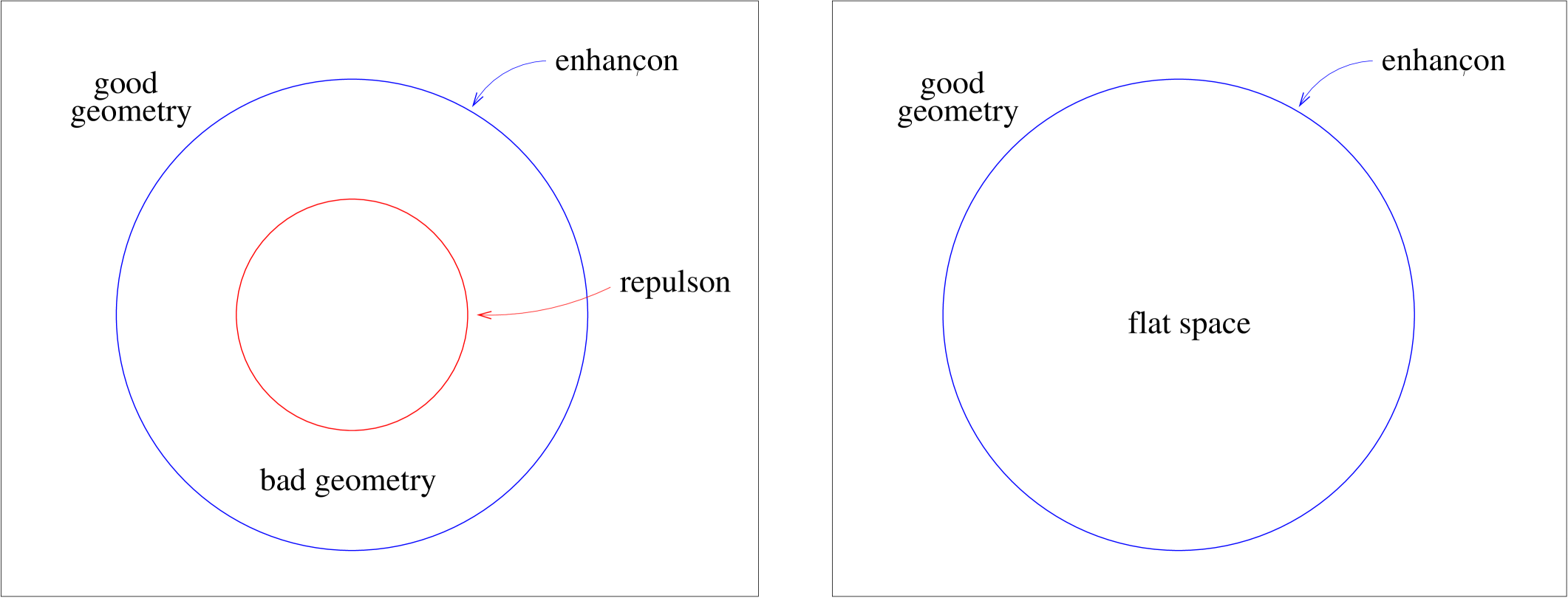
Figure 1: Left: A slice through the enhançon (exterior) and repulson (interior) loci. Right: The geometry after excision. (The situation is spherically symmetric and the three dimensional loci are constructed by revolving the plot about the vertical axis.)

The resulting complete geometry is well–behaved, possessing the correct physical properties to match certain gauge theory phenomena expected from the world–volume theory on the branes, such as the metric on moduli space. The configuration has eight supercharges, which is enough to have a moduli space, but not so much as to force it to be trivially flat.

The proposal to excise the bad region and replace it with flat space, while a natural one, might have seemed considerably drastic from other points of view, and one might ask whether it is a consistent procedure from the purely supergravity perspective: Since the enhanced gauge symmetry is a purely stringy phenomenon, is there any sense in which the excision procedure is natural in supergravity? After doing a purely supergravity analysis[6], the satisfying answer is that the excision is not only allowed by the supergravity (in fact, one can perform it at any radius greater than $r_{\rm e}$ in that spherical case and get sensible results), but it is extremely natural to carry it out at the enhançon radius. The reason is as follows: One glues the exterior geometry onto the new interior (flat space) and any mismatch in the extrinsic curvatures of the geometries across the junction acts as a source in the theory, which in this case would be the smeared shell of branes. The analysis of ref.[6] (see also ref.[7]) showed that the shell of branes was in fact massless at the enhançon radius, consistent with the superstring expectations given above. Furthermore, the enhançon radius was the most economical place at which to perform the excision, since that radius also coincided with the outermost reaches of the unphysical repulsive interior region, as could be seen by probing with ordinary supergravity test particles.

While this special spherically symmetric situation is compelling, it is interesting to find more examples, and explore the nature of the mechanism in greater detail. The spherical symmetry is quite seductive, and it is easy to forget that there should be nothing particularly special about that symmetry. After all, the $N$ constituent branes are BPS, and so in fact as long as we do not develop any unphysical regions, very many shapes should be possible, and for large $N$, almost any shape is imaginable. The difficulty is of course in finding supergravity techniques which facilitate the exhibition of solutions describing the non–trivial shapes that we can imagine.

For this project we set out to do the most simple BPS deviation from the sphere we could think of, which was to deform to an oblate situation, and perhaps work perturbatively away from the spherical situation. To our surprise, the result was much richer than we could have hoped for. We succeed in describing a complete family of axially symmetric geometries, parametrised by a parameter $\ell$. It transpires that there is a critical value, $\ell^{\rm cr}_{\rm e}$, separating two distinct physical situations. The reader should refer to figure 2 (on page 2) which illustrates the following descriptions:

• For $\ell<\ell^{\rm cr}_{\rm e}$, the enhançon locus is disconnected: There is an outer shell and an inner shell, with non–trivial supergravity inside the inner shell. The region between the two shells is unphysical in the naive geometry and is excised and replaced by flat space, while the region inside the inner shell is perfectly well–behaved, and so remains. For increasing $\ell$ the outer shell becomes more depressed at the poles, forming an oblate shape, while the inner shell reaches increasingly outwards towards the poles.

• Even more remarkably, perhaps, for $\ell=\ell^{\rm cr}_{\rm e}$, the two enhançon shells join, and the enhançon is no longer disconnected. For $\ell>\ell^{\rm cr}_{\rm e}$, the complete enhançon locus is in fact a torus. The torus flattens increasingly for greater $\ell.$ See also figure (3).

• Another choice which can be made for $\ell<\ell^{\rm cr}_{\rm e}$ is to excise the entire interior, leaving the oblate shape outside, and flat space in the entire interior region.

Remarkably, the supergravity excision technology is tractable in this situation, and confirms that these are physically sensible choices.

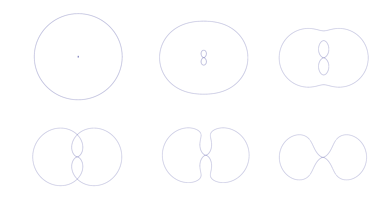
Figure 2: A series of slices through the enhançon loci for varying values of a parameter $\ell$. The three dimensional loci are constructed by revolving the plots about the vertical axis. The first one is closest to the spherical case, $\ell=0$ in figure 1. Here, there is a small interior enhançon locus at the origin. For $0<\ell<\ell^{\rm cr}_{\rm e}$, the enhançon locus is in general disconnected, the interior shape being steadily more visible with increasing $\ell$, and the outer shell becomes increasingly oblate until at $\ell=\ell^{\rm cr}_{\rm e}$, they touch, forming a single shape, which persists as a torus for $\ell>\ell_{\rm cr}^{\rm e}$. (Later, we shall see that the point in the centre is indeed a hole.)

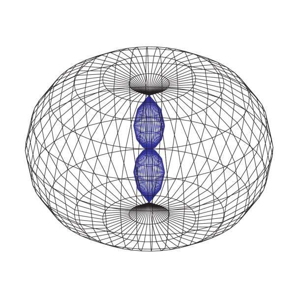
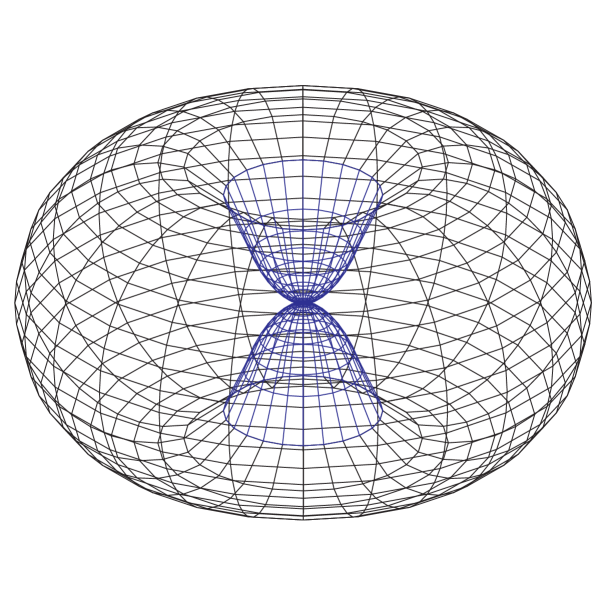
Figure 3: A three dimensional depiction of the connected enhançon locus, at $\ell=\ell^{\rm cr}_{\rm e}$ (left), and $\ell>\ell^{\rm cr}_{\rm e}$ (right).

In this paper we report on this interesting and highly non–trivial example of supergravity geometry as an exhibit of the enhançon mechanism at work, and as a study which allows us to learn more about certain brane configurations. In section 2, we study first a generalised six–brane supergravity solution which corresponds to a disc distribution of D6–branes. Such branes are the nicest geometries to wrap on K3, since the remaining transverse geometry has three spatial dimensions. This means that the resulting geometry is easy to visualise, and, at a deeper level, much of the mathematics is quite familiar, as we shall see. There are two useful coordinate systems which are employed here to uncover aspects of the geometry in the wrapped case, and it is worthwhile exploring them in the unwrapped case. The unwrapped case itself is interesting, and we compare it to expressions that we derive for other D–brane disc distributions.

We should make a cautionary note, however. It is useful to describe these solutions in terms of a continuous density of branes. While this is a simplification, (since branes come in discrete amounts due to charge quantisation), it is a good and useful approximation at large $N$. However, the D6–brane disc distribution that we find has the strange feature that the density function in the interior of the disc is in fact negative, which is hard to interpret. However, we are able to characterise the behaviour resulting from this strange feature and do not discard the solution, for at least three reasons:

• Apart from the negative density itself, there is no compelling reason to think that there might not be yet to be found some beyond–supergravity means of explaining the role of such a geometry, perhaps involving something analogous to the enhançon mechanism.

• The negative density has nothing to do with the repulson geometry arising from wrapping, which is what we really want to study in this paper. We need not “throw out the baby with the bathwater”, and can carry out a separate discussion of the wrapping and its associated features, including the enhançon mechanism. The features associated to this negative density are clearly isolated in the discussion and do not play any role.

• The D5– and D4–brane distributions which we also display have no such strange behaviour, and the subsequent discussion of the appearance of the repulson after wrapping and its resolution by the enhançon is similar in spirit to the D6–brane case we study in detail first. Even if the D6–brane example we study here does not turn out to be salvageable in its entirety, we will see that the key features survive in these better–behaved examples.

In short, we can use the D6–brane case as a (rather pretty) simple model, and be aware of the negative density, but not distracted by it, leaving its understanding for another day.

We also exhibit the fact that the behaviour of the harmonic functions corresponding to the distribution has a beautiful expansion in terms of Legendre polynomials. Recalling that the moduli space of the wrapped brane system is isomorphic to that of the Coulomb branch of the ${\cal N}=4$ supersymmetric $(2+1)$–dimensional pure $SU(N)$ gauge theory, this will yield a useful geometrical parametrisation of the vacuum expectation values of operators made from the symmetric product of the three adjoint scalars in the gauge multiplet, an issue we return to in section 6.

In section 3 we uncover the properties of the wrapped system, seeking the repulson and enhançon loci, and characterising them, displaying the equations which result in figures 2 and 3. We probe the supergravity solution with wrapped branes and point particles, in order to discover the nature of the unphysical regions of the geometry. We then perform the excision to construct new geometries which are free of the repulson regions arising from the wrapping, checking consistency in supergravity in section 4. In section 5 we discuss some features of wrapped D4– and D5–brane distributions. Section 6 extracts some gauge theory results from the D6–brane case. We conclude with some remarks in section 7.

2 D–Brane Distributions

It is possible to derive a metric for a continuous distribution of branes by taking extremal limits of rotating solutions. The limits remove the rotation and restore supersymmetry, and the parameters that corresponded to rotation remain in the geometry as parameters of the distribution (for D3–branes this was done first in refs.[10, 11]). We can do this here for D6–branes as follows: The rotating black six–brane solution, in the usual supergravity conventions, is given by:

$$ds^{2} = {\hat{f}}_{6}^{-1/2}\Big{(}-K~{}dt^{2}+\sum_{i=1}^{6}dx_{i}^{2}\Big{)}+{\hat{f}}_{6}^{1/2}\Big{(}\bar{K}^{-1}\frac{\Delta}{\Xi}~{}dr^{2}+\Delta r^{2}~{}d\theta^{2}+\Xi r^{2}\sin^{2}\theta~{}d\phi^{2}\Big{)}$$

$$+{\hat{f}}_{6}^{-1/2}\frac{2m}{\Delta r}\Big{(}\ell^{2}\sin^{4}\theta~{}d\phi^{2}-2\cosh\delta~{}\ell\sin^{2}\theta~{}dtd\phi\Big{)}\ ,$$

$$e^{2\Phi} = {\hat{f}}_{6}^{-3/2},$$

$$C_{7} = \frac{1}{\sinh\delta}{\hat{f}}_{6}^{-1}\Big{(}\cosh\delta~{}dt-\ell\sin^{2}\theta~{}d\phi\Big{)}\wedge dx_{1}\wedge\ldots\wedge dx_{6}\ ,$$ (1)

where

$${\hat{f}}_{6}=1+\frac{2m\sinh^{2}\delta}{\Delta r}\ ,\qquad\qquad K=1-\frac{2m}{\Delta r}\ ,\qquad\qquad\bar{K}=1-\frac{2m}{\Xi r}\ ,$$ (2)

and

$$\Delta=1+\frac{\ell^{2}}{r^{2}}\cos^{2}\theta\ ,\qquad\qquad\Xi=1+\frac{\ell^{2}}{r^{2}}\ ,$$ (3)

while $r$ is a radial coordinate for three Cartesian coordinates $x_{7},x_{8},x_{9}$ with $r^{2}=x_{7}^{2}+x_{8}^{2}+x_{9}^{2}$ and we are using standard spherical polar coordinates such that $x_{9}=r\cos\theta$, and so on.

We can obtain an extremal limit by sending the non–extremality parameter $m\rightarrow 0$ and the boost parameter $\delta\rightarrow\infty$, while keeping $r_{6}=2m\sinh^{2}\delta$ fixed. In this limit the metric component, $g_{t\phi}$, giving rise to rotation does not survive and the resulting solution is:

$$ds^{2} = f_{6}^{-1/2}\Big{(}-dt^{2}+\sum_{i=1}^{6}dx_{i}^{2}\Big{)}+f_{6}^{1/2}\Big{(}\frac{\Delta}{\Xi}~{}dr^{2}+\Delta r^{2}~{}d\theta^{2}+\Xi r^{2}\sin^{2}\theta~{}d\phi^{2}\Big{)}\ ,$$

$$e^{2\Phi} = f_{6}^{-3/2},$$

$$C_{7} = f_{6}^{-1}dt\wedge dx_{1}\wedge\ldots\wedge dx_{6}\ ,$$ (4)

where

$$f_{6}=1+\frac{r_{6}}{\Delta r}\ .$$ (5)

This can be done for the other solutions presented in refs.[12, 10, 13] as well, giving distributions of other D$p$–branes, and we refer to some of the results of this later.

The normalisation $r_{6}=gN\alpha^{\prime 1/2}/2$ gives $N$ units of D6–brane charge, $\mu_{6}=(2\pi)^{-6}\alpha^{{}^{\prime}-7/2}$, in the standard units [14]. In the next section we wrap this configuration of D6–branes on K3. However, let us first examine the structure of this configuration, in order to understand better what new features are specifically brought about by the wrapping, and which are due to the distribution’s geometry.

The parameter $\ell$ controls the departure from a spherical geometry. In the case $\ell=0$, the solution in equation (4) reduces to the usual spherically symmetric static D6–brane solution[15], where the singularity at $r=0$ is interpreted as the position where the branes reside. Now, as soon as $\ell\neq 0$, that singularity disappears except for on the equatorial plane $\theta=\pi/2$: The denominator in the harmonic function is now $r+(\ell^{2}/r)\cos^{2}\theta$, which only vanishes at $r=0,\theta=\pi/2$, so the source at $r=0$ has been modified. Let us try to understand how.

To get a better understanding of the source, let us perform the following transformation[12] to isotropic coordinates which we shall refer to as “extended”:

$$y_{1} = \sqrt{r^{2}+\ell^{2}}\,\sin\theta\,\cos\phi\ ,$$

$$y_{2} = \sqrt{r^{2}+\ell^{2}}\,\sin\theta\,\sin\phi\ ,$$

$$y_{3} = r\,\cos\theta\ .$$ (6)

We see that the origin $r=0$ is mapped to a disc, given by $y_{1}^{2}+y_{2}^{2}=\ell^{2}\sin^{2}\theta$, $y_{3}=0$. Going to $r=0$ along $\theta=0$ takes us to the centre of the disc at $y=0$, while an approach along $\theta=\pi/2$ takes us to the edge of the disc at $y_{1}^{2}+y_{2}^{2}=\ell^{2}$. Approaching along other angles takes us to the interior of the disc.

The metric in equation (4) reduces to a standard brane form:

$$ds^{2}=F_{6}^{-1/2}\Big{(}-dt^{2}+\sum_{i=1}^{6}dx_{i}^{2}\Big{)}+F_{6}^{1/2}\Big{(}dy_{1}^{2}+dy_{2}^{2}+dy_{3}^{2}\Big{)}\ ,$$ (7)

where the harmonic function is given by

$$F_{6}=1+\frac{r_{6}\sqrt{\Lambda+\Sigma}}{\sqrt{2}\Sigma}\ ,$$ (8)

with

$$\Sigma=\sqrt{\Lambda^{2}+4\ell^{2}y_{3}^{2}}\ ,\qquad\Lambda=y^{2}-\ell^{2}\ ,\qquad y=\sqrt{y_{1}^{2}+y_{2}^{2}+y_{3}^{2}}\ .$$ (9)

Now we see that the singularity we identified earlier is in fact a ring of radius $\ell$. Is this where the branes are located? The harmonic function $F_{6}$ should have an integral representation given schematically by

$$F_{6}=1+\int{\frac{\sigma(y^{\prime})}{|y-y^{\prime}|}dy^{\prime}}\ ,$$ (10)

for some density function $\sigma(y)$ representing a continuous distribution of branes in the coordinate $y$. How seriously we should take the physical meaning of this distribution is a matter of interest. For many applications, of concern to supergravity quantities, the meaning of a continuous distribution of branes should not be a problem, but we must remember that in the full string theory, we might wish to probe the structure of the solution at resolutions which might render the distribution meaningless.

It is possible to directly determine the distribution’s dependence on $y$, using an analogue of Gauss’ Law. For six–branes, we have three transverse spatial dimensions, and so the problem of determining harmonic functions is in fact directly translated into an undergraduate electromagnetism problem.

Let us define $\rho=\sqrt{y_{1}^{2}+y_{2}^{2}}$, $z=y_{3}$. It is sufficient to determine the harmonic function’s behaviour along the $z$–axis. The density function and the angular dependence of $F_{6}$ follows directly from harmonic analysis. The analogue of Gauss’ law in electrodynamics for a standard infinitesimal “pillbox” surface defined on the $z=0$ plane is:

$$({\vec{E}}_{+}-{\vec{E}}_{-})\cdot{\vec{n}}=4\pi\sigma\ ,$$ (11)

where ${\vec{n}}$ is the unit normal vector of the surface directed from one side ($-$) to the other side ($+$) of the surface, and $\sigma$ is the surface charge density. The electric field is ${\vec{E}}=-{\vec{\nabla}}\Phi$, while the role of the potential $\Phi$ is now played by the harmonic function. Taking the derivative,

$$\frac{\partial F_{6}}{\partial z}=\frac{zr_{6}}{\sqrt{2}\Sigma^{3}\sqrt{\Lambda+\Sigma}}\Big{(}\Sigma^{2}-\Lambda\Sigma-2\Lambda^{2}-2\ell^{2}(2\Lambda+\Sigma)\Big{)}\ ,$$ (12)

we obtain

$$\sigma(\rho)=\frac{1}{4\pi}\left(\frac{\partial F_{6}}{\partial z}\Big{|}_{z\rightarrow 0^{-}}-\frac{\partial F_{6}}{\partial z}\Big{|}_{z\rightarrow 0^{+}}\right)=-\frac{r_{6}\ell}{2\pi(\ell^{2}-\rho^{2})^{3/2}}\ ,$$ (13)

where an expansion in small $z$ was used to get this result. This density is negative, but happily (since it would be hard to see how to get a positive result for the D6–brane charge from this), it integrates to infinity over the disc, due to the boundary contribution. We must therefore add an extra positive term to the boundary, so that the complete distribution is

$$\sigma(y)=-\frac{r_{6}\ell}{2\pi(\ell^{2}-\rho^{2})^{3/2}}\Theta(\ell-\rho)\delta(z)+\frac{r_{6}}{2\pi\sqrt{\ell^{2}-\rho^{2}}}\delta(\ell-\rho)\delta(z)\ .$$ (14)

It is worth checking that the normalisation of the configuration is indeed $r_{6}$ as expected

$$\int_{0}^{\ell}2\pi\sigma(\rho)\rho d\rho = \int_{0}^{\ell}\Big{(}-\frac{r_{6}\ell\rho}{(\ell^{2}-\rho^{2})^{3/2}}+\frac{r_{6}\rho}{\sqrt{\ell^{2}-\rho^{2}}}\delta(\ell-\rho)\Big{)}d\rho$$ (15)

$$= \left[-\frac{r_{6}\ell}{\sqrt{\ell^{2}-\rho^{2}}}\right]_{\rho=0}^{\rho=\ell}+\left.\frac{r_{6}\rho}{\sqrt{\ell^{2}-\rho^{2}}}\right|_{\rho=\ell}=r_{6}\ ,$$

and that the brane distribution (14) correctly reproduces our harmonic function along the $z$–axis:

$$F_{6} = 1+2\pi\int_{0}^{\ell}\frac{\sigma(\rho)\rho d\rho}{\sqrt{z^{2}+\rho^{2}}}$$ (16)

$$= 1+\int_{0}^{\ell}\left(-\frac{r_{6}\ell\rho}{\sqrt{z^{2}+\rho^{2}}(\ell^{2}-\rho^{2})^{3/2}}+\frac{r_{6}\rho}{\sqrt{z^{2}+\rho^{2}}\sqrt{\ell^{2}-\rho^{2}}}\delta(\ell-\rho)\right)d\rho$$

$$= 1+\left[-\frac{r_{6}\ell}{(\ell^{2}+z^{2})}\frac{\sqrt{z^{2}+\rho^{2}}}{\sqrt{\ell^{2}-\rho^{2}}}\right]_{\rho=0}^{\rho=\ell}+\left.\frac{r_{6}\rho}{\sqrt{z^{2}+\rho^{2}}\sqrt{\ell^{2}-\rho^{2}}}\right|_{\rho=\ell}=1+\frac{r_{6}z}{\ell^{2}+z^{2}}\ .$$

This is very interesting, particularly when compared to the results (listed in equation (17)) one can get by computing the analogous quantities for D$p$–brane disc distributions for $p=0,\cdots 5$. The results are easy to obtain by noting first that along the $z$ axis, the harmonic function’s form in extended coordinates is exactly the same as in unextended coordinates:

$$f=1+\frac{r_{p}^{7-p}}{z^{7-p}\left(1+{\ell^{2}}/{z^{2}}\right)}\ .$$

This can be verified by simply examining the appropriate metrics, which can be derived by taking an extremal limit of the metrics listed in [13], as we did for equation (1) to get equation (4), keeping only one non–zero parameter $\ell_{1}=\ell$. Given that the harmonic function should have an integral representation

$$f=1+\int\frac{\sigma(y^{\prime})dy^{\prime}}{|y-y^{\prime}|^{7-p}}\ ,$$

it is easy to guess the densities in each case and check them by explicit integration. We list the densities here, and plot them in figure 4:

$${\rm D0}: \sigma(y)\ =\ +\frac{5r_{0}^{7}}{2\pi\ell^{5}}\ (\ell^{2}-\rho^{2})^{\frac{3}{2}}\ \Theta\,(\ell-\rho)\ \delta(z)\ ,$$

$${\rm D1}: \sigma(y)\ =\ +\frac{4r_{1}^{6}}{2\pi\ell^{4}}\ (\ell^{2}-\rho^{2})^{1}\ \Theta\,(\ell-\rho)\ \delta(z)\ ,$$

$${\rm D2}: \sigma(y)\ =\ +\frac{3r_{2}^{5}}{2\pi\ell^{3}}\ (\ell^{2}-\rho^{2})^{\frac{1}{2}}\ \Theta\,(\ell-\rho)\ \delta(z)\ ,$$

$${\rm D3}: \sigma(y)\ =\ +\frac{2r_{3}^{4}}{2\pi\ell^{2}}\ (\ell^{2}-\rho^{2})^{0}\ \Theta\,(\ell-\rho)\ \delta(z)\ ,$$

$${\rm D4}: \sigma(y)\ =\ +\frac{r_{4}^{3}}{2\pi\ell}\ (\ell^{2}-\rho^{2})^{-\frac{1}{2}}\ \Theta\,(\ell-\rho)\ \delta(z)\ ,$$

$${\rm D5}: \sigma(y)\ =\ \hskip 152.22241pt+\frac{r_{5}^{2}}{2\pi}\ (\ell^{2}-\rho^{2})^{0}\delta(\ell-\rho)\ \delta(z)\ ,$$

$${\rm D6}: \sigma(y)\ =\ -\frac{r_{6}\ell}{2\pi}(\ell^{2}-\rho^{2})^{-{3\over 2}}\Theta(\ell-\rho)\delta(z)+\frac{r_{6}}{2\pi}(\ell^{2}-\rho^{2})^{-{1\over 2}}\delta(\ell-\rho)\delta(z)\ .$$ (17)

(Now $z$ in the above is shorthand for all of the directions transverse to the disc and, of course, to the brane’s world–volume.) The pattern is amusing. For a D$p$–brane, as $p$ becomes larger, the distribution increasingly spreads away from the centre. The D5–brane case is a limiting one, having all of the branes at the boundary forming a ring. The D6–brane case (not plotted) also has a $\delta$–function on the boundary, but is accompanied by a negative contribution to $\sigma(y)$ in the interior.

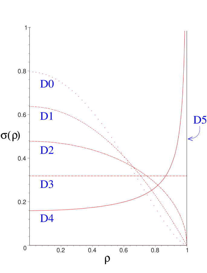
Figure 4: Disc density distributions of D$p$–branes in a plane for $p=0,\cdots 5$, normalised to the same area. The case of D5–branes is a delta function on the edge, at $\rho=1$. The amusing pattern followed by these distributions is described in the text.

While there is a striking pattern here, we must pause to consider what the physical significance of the negative contribution to the distribution of branes might be. As we said previously, we must be careful about the meaning of the continuous distribution in general, since it is merely a supergravity approximation. However, the negative density (and hence tension and charge) is somewhat harder to accept, and may be another cry for help from the supergravity, appealing to more stringy physics to resolve the problem.

This is of course reminiscent of the features which are resolved by the enhançon mechanism. There is a region where branes seem to have negative tension. In that case[1] this was seen by sending in a probe brane of the same type to the affected region. The supergravity geometry in the interior was consequently discarded because one could argue that it can not be constructed by bringing all of the constituent branes from infinity. We can not apply that reasoning here, however. A probe D6–brane will again see no potential for movement in this background, and the resulting moduli space metric is perfectly flat right down to $y=0$. So it would seem that we can not argue in this way that we can’t construct this supergravity solution.

Later, we will also see that this sort of distribution corresponds to switching on apparently sensible vacuum expectation values for gauge theory operators. That discussion will be aided by noting that the harmonic function $F_{6}$ can be expanded in a series in the variable ${\ell}/{y}$ for $y>\ell$, or ${y}/{\ell}$ for $y<\ell$. It is delightful to see how these series arrange themselves in terms of Legendre polynomials:

$$F_{6} = 1+\frac{r_{6}}{y}\sum_{n=0}^{\infty}(-1)^{n}\left(\frac{\ell}{y}\right)^{2n}P_{2n}(\cos\ \hat{\theta})\ ,\qquad y>\ell\ ,$$ (18)

$$F_{6} = 1+\frac{r_{6}}{\ell}\sum_{n=0}^{\infty}(-1)^{n}\left(\frac{y}{\ell}\right)^{2n+1}P_{2n+1}(\cos\ \hat{\theta})\ ,\qquad y<\ell\ ,$$ (19)

where we have defined new polar coordinate angles with respect to the $y_{i}$’s:

$$\hat{\theta} = \cos^{-1}\left(\frac{y_{3}}{y}\right)\ ,$$

$$\hat{\phi} = \tan^{-1}\left(\frac{y_{2}}{y_{1}}\right)=\phi\ ,$$ (20)

and $P_{n}(x)$’s are the Legendre polynomials in the variable $x$, with the normalisation:

$$P_{0}(x)=1\ ;\quad P_{1}(x)=x\ ;\quad P_{2}(x)=\frac{1}{2}(3x^{2}-1)\ ;\quad{\rm{\it etc}.}$$ (21)

In hindsight, this is of course what we should expect from a direct expansion of equation (16), combined with harmonic analysis.

It is worth noting that we can insert any of our favourite harmonic potentials from electromagnetism (or higher dimensional generalisations) and get a supergravity solution corresponding to a distribution of D–branes. This could in principle be wrapped on K3, as we do in section 3. However, since these are most commonly found as a series expansion of the form above, exact determination of the crucial enhançon and repulson loci (as we do later) will not in general be possible.

2.1 Particle Probes of the Geometry

It is interesting to probe the system with a point particle using the standard technology. There are Killing vectors $\mathbf{\xi}=\partial/\partial t$ and ${\bf\eta}=\partial/\partial\phi$ which, for a particle moving on timelike geodesics, with velocity ${\bf u}$, define for us conserved quantities $e=-{\bf\xi}\cdot{\bf u}$ and $L={\bf\eta}\cdot{\bf u}$. In terms of these, we can write a first integral of the geodesic equation. The purely radial motion on the equatorial plane or along the symmetry axis (i.e., assuming ${\bf u}^{\theta}=0$, and ${\bf u}^{\phi}=0$) of the test particle is described by

$$\frac{\Delta}{\Xi}\dot{r}^{2}=E-V_{\rm eff}(r)\ .$$ (22)

The effective potential that the particle probe feels is

$$V_{\rm eff}(r)=-\frac{1}{2}\left(g_{tt}+1\right)\ .$$ (23)

We plot $V_{\rm eff}$ for a particle approaching along the equator and also along the $z$–axis in figure 5. It is interesting to note that accompanying this negative brane region is a repulsive behaviour in the supergravity. A test particle located along the $z$–axis sees a potential which is repulsive inside a radius $\ell$. This has nothing to do with the repulson singularity coming from wrapping, which we will study shortly, so we must bear in mind that it is a feature which will descend from the unwrapped configuration to the wrapped configuration. Later, in section 5, we shall see that there is no such behaviour for D5–brane distributions, and so we will treat this as an artifact of the D6–brane case in what follows, as it will not affect our analysis of the excision of the repulson behaviour arising from wrapping.

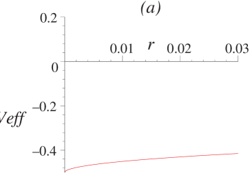
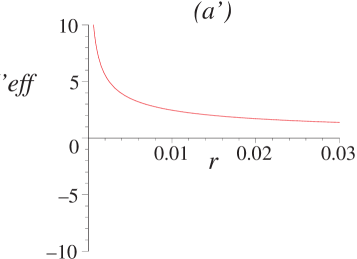
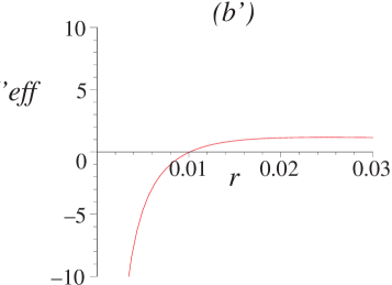
Figure 5: Gravitational features of the unwrapped D6–brane distribution as seen by a neutral test particle. The test particle effective potential (left) and its derivative (right) along the axis of symmetry ($\theta=0$) corresponding to (a) $\ell=0$, (b) $\ell>0$. In the latter case the potential becomes repulsive at a distance $\ell$ from the origin. The effective potential for a particle moving on the equatorial plane ($\theta=\pi/2$) is always attractive, and is similar to case (a).

3 Wrapping the D6–Branes

We have learned enough about our configuration to return to our problem of wrapping the branes on K3. Wrapping a D6–brane on K3 induces precisely one unit of negative D2 brane charge in the D6–brane world–volume. As in ref.[1], this suggests that the appropriate supergravity solution is that appropriate to a D6–brane with delocalised D2–branes in its world–volume[17], where in the D2–brane harmonic function, we put $r_{2}=-r_{6}V_{\star}/V$, where $V$ is the volume of K3 as measured at infinity and $V_{\star}=(2\pi)^{4}\alpha^{\prime 2}$. This leads to the following geometry (we remind the reader here that there are no real D2–branes in the geometry):

$$ds^{2} = f_{2}^{-1/2}f_{6}^{-1/2}(-dt^{2}+dx_{1}^{2}+dx_{2}^{2})+f_{2}^{1/2}f_{6}^{1/2}\left(\frac{\Delta}{\Xi}\,dr^{2}+\Delta r^{2}\,d\theta^{2}+\Xi\,r^{2}\sin^{2}\theta\,d\phi^{2}\right)$$ (24)

$$\hskip 85.35826pt+V^{1/2}f_{2}^{1/2}f_{6}^{-1/2}ds_{K3}^{2}\ .$$

with

$$f_{2}=1-\frac{r_{6}V_{\star}}{V\Delta r}\ ,\quad f_{6}=1+\frac{r_{6}}{\Delta r}\ ,$$ (25)

$ds_{K3}^{2}$ is the metric of a unit volume K3 surface, and the functions $\Delta$ and $\Xi$ were defined before. The dilaton and R–R fields are given by

$$e^{-2\Phi} = \left(\frac{f_{6}^{3}}{f_{2}}\right)^{1/2}\ ,$$

$$C^{(3)} = \frac{1}{f_{2}}dt\wedge dx_{1}\wedge dx_{2}\ ,$$

$$C^{(7)} = \frac{1}{f_{6}}dt\wedge dx_{1}\wedge dx_{2}\wedge Vds_{K3}\ .$$ (26)

Despite being a solution to the supergravity equations of motion, the geometry for this configuration is not consistent. Naked singularities (seen e.g. by examining the curvature invariants $R$, $R_{\mu\nu}R^{\mu\nu}$, $R_{\mu\nu\rho\sigma}R^{\mu\nu\rho\sigma}$, etc.) of repulson[2] type appear where the running K3 volume, given by:

$$V(r,\theta)=V\frac{f_{2}}{f_{6}}\ ,$$ (27)

shrinks to zero. Some algebra shows that this occurs at radii:

$$r_{\rm r}=\frac{r_{6}V_{\star}}{2V}\left[1\pm\left(1-\frac{4V^{2}}{r_{6}^{2}V_{\star}^{2}}\ell^{2}\cos^{2}\theta\right)^{1/2}\right].$$ (28)

When $\ell$ is zero, we have the spherically symmetric situation where the singularity appears on a sphere of radius ${r_{6}V_{\star}}/{V}$. For non–zero, but sufficiently small $\ell$ the singularity appears at two disconnected loci, one of them inside the other, and between these loci the metric (24) is imaginary. When $\ell$ reaches the critical value

$$\ell^{\rm cr}_{\rm r}=\frac{r_{6}V_{\star}}{2V}\ ,$$ (29)

these two surfaces meet and join into one single surface for $\ell>\ell^{\rm cr}_{\rm r}$.

We expect stringy effects to have switched on long before a vanishing volume is reached, since when the volume gets to the value $V_{\star}$, there are extra massless states coming from wrapped D4– and anti–D4–branes, giving an enhanced $SU(2)$ in spacetime. The radius at which this occurs is the enhançon radius, and it is easily computed to give:

$$r_{\rm e}=\frac{r_{6}V_{\star}}{V-V_{\star}}\left[1\pm\left(1-\frac{(V-V_{\star})^{2}}{r_{6}^{2}V_{\star}^{2}}\ell^{2}\cos^{2}\theta\right)^{1/2}\right]\ .$$ (30)

This is of course the same radius that gives a zero of the effective tension of a probe wrapped D6–brane, whose action is[1, 14]:

$$S=-\int d^{3}\xi\,\,\mu_{6}e^{-\Phi}\left(V(r)-V_{\star}\right)(-\det g_{ab})^{1/2}+\mu_{6}\int C^{(7)}-\mu_{2}\int C^{(3)}\ ,$$ (31)

where $\xi^{a}$ $(a,b=0,1,2)$ are the coordinates on the unwrapped part of the world–volume and $g_{ab}$ is the induced metric. Working in static gauge the potential vanishes and we obtain the result for the effective Lagrangian:

$${\cal L}=\frac{\mu_{6}}{2g_{s}}(Vf_{2}-V_{\star}f_{6})\,\left(\frac{\Delta}{\Xi}\ \dot{r^{2}}+\Delta r^{2}\ \dot{\theta^{2}}+\Xi\,\,r^{2}\sin^{2}\theta\ \dot{\phi}^{2}\right)\ ,$$ (32)

and we can read off the effective mass (tension) as

$$\tau_{\rm eff}=\frac{\mu_{6}}{g_{s}}f_{6}\left(V\frac{f_{2}}{f_{6}}-V_{\star}\right)\ .$$ (33)

Let us study the enhançon radius given in equation (30). For $\ell=0$ we recover the spherically symmetric case with enhançon radius ${2r_{6}V_{\star}}/({V-V_{\star}})$. For non–zero $\ell$, two different situations can be observed, depending on whether $\ell$ is smaller or greater than the critical value:

$$\ell_{\rm e}^{\rm cr}\ =\ \frac{r_{6}V_{\star}}{V-V_{\star}}\ .$$ (34)

When $\ell\leq\ell_{\rm e}^{\rm cr}$, there are two enhançon shells which divide our geometry into three distinct regions. The tension of a D6–brane probe drops to zero at the outer enhançon shell. Let us call the exterior region of positive tension region I. In between the outer and inner enhançon shells, the tension of our probe would be negative. We will call this region II. This is the region where we encountered the repulson singularities (28) and it will be excised shortly. Finally, the tension is again positive in region III, inside the inner enhançon shell. We can be sure that singularities are contained in the region II only, because the running K3 volume is a continuous function and $V_{\star}>0$. The origin $r=0$, appears to be problematic, since it solves both equation (28) and equation (30). In fact, if we approach $r=0$ along the $z$–axis, we get $V(r,\theta)\to V$ while an approach along the equator shows that $V(r,\theta)\to-V_{\star}$, which is puzzling. This is partly resolved by going to the extended coordinates, where $r=0$ opens up into a disc. Then we see that $V(r,\theta)\to-V_{\star}$ as we approach the edge of the disc, while $V(r,\theta)=V$ on the interior of the disc.

Notice what happens when $\ell=\ell_{\rm e}^{\rm cr}$. The inner and outer enhançon shells meet at two points on the $z$–axis. The tension of a brane probe moving along this axis drops to zero at the enhançon radius and becomes positive again.

For $\ell>\ell_{\rm e}^{\rm cr}$, the inner and outer enhançon shells have merged into a single connected shell with a toroidal shape. Our geometry is now divided into two distinct regions. The volume of K3 is less than $V_{\star}$ in the interior of the torus. The repulson singularities lie inside the torus. Actually, although there is no physical significance to the fact, it is worth noting that the repulson loci undergo a similar evolution from disconnected to connected (with the critical value $\ell_{\rm r}^{\rm cr}$ separating the two cases), with shapes of the same sort. Since $\ell_{\rm r}^{\rm cr}<\ell_{\rm e}^{\rm cr}$, the repulson always becomes connected before the enhançon locus does.

This all seems rather complicated, but is quite beautiful to look at, in fact. We have already sketched the enhançon loci in figures 2 and 3, but now we put it together with the repulson loci by shading in dark grey (or blue for viewers in colour) in the regions where the volume is greater than zero but less than $V_{\star}$ in figure 6, for different values of $\ell$. The light (or yellow) regions are volumes greater than $V_{\star}$, and so the boundary between these is the enhançon locus. The black region is for negative volumes, in other words, where the metric does not exist. The boundary between it and the grey (blue) is the repulson locus.

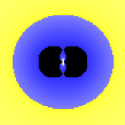
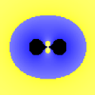
Figure 6: A vertical slice through the non–spherical wrapped D6–brane geometry before excision. The origin $r=0$ is placed in the centre of the figure. The symmetry axis, $\theta=0$, corresponds to the vertical direction and $\theta=\pm{\pi}/{2}$ to the horizontal. The region where the K3 volume $V(r,\theta)<0$ is black. The region where $0\leq V(r,\theta)<V_{\star}$ is dark grey (blue). The repulson radius $r_{\rm r}$ is marked by the border between these two regions. The physically acceptable region $V(r,\theta)\geq V_{\star}$, where the tension of the probe brane is positive, is in the light shade (different shades between yellow ($V(r,\theta)$ is close to $V_{\star}$) and white ($V(r,\theta)$ is close to $V$)). The enhançon radius $r_{\rm e}$ is the border between the dark grey (blue) and the light regions. $\ell=0$ gives a spherical enhançon. For increasing values of $\ell$, two disconnected shells appear forming a double enhançon. Once $\ell^{\rm cr}_{\rm e}$ is exceeded, the two shells join forming a single enhançon. This pattern can be seen explicitly in the figure for the following values of $\ell$ : $\ell=0$ (top, left), $\ell=\frac{1}{2}\ell^{\rm cr}_{\rm r}$, $\ell=\ell^{\rm cr}_{\rm r}$, $\ell=\ell^{\rm cr}_{\rm e}-\frac{1}{2}(\ell^{\rm cr}_{\rm e}-\ell^{\rm cr}_{\rm r})$ (top, right), $\ell=\ell^{\rm cr}_{\rm e}$ (bottom, left), $\ell=\frac{9}{8}\ell^{\rm cr}_{\rm e}$, $\ell=2\ell^{\rm cr}_{\rm e}$, $\ell=8\ell^{\rm cr}_{\rm e}$ (bottom, right). Other parameters $r_{6}$, $V$, and $V_{\star}$ have been fixed to some typical values.

One may wonder what happens to the enhançon if we transform the solution (24) into the “extended” coordinates given in equations (6). In these coordinates, essentially the same features arise. The singular region where the K3 volume shrinks to zero is surrounded by the enhançon shell(s). The same critical value of the parameter $\ell$ separates two families of enhançons as before. We re–plot the K3 volume in the extended coordinates in figure 7.

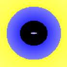
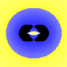
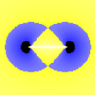
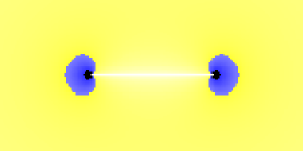
Figure 7: A slice through the untreated wrapped D6–brane geometry in “extended” coordinates. The colour coding is the same as in figure 6. The case $\ell=0$ gives a spherical enhançon. For increasing values of $\ell$, two disconnected enhançon shells appear forming coconut shape. Once $\ell^{\rm cr}_{\rm e}$ is exceeded, the two enhançon shells join to form a torus. This pattern can be seen for the following values of $\ell$ :  $\ell=0$ (top, left), $\ell=\frac{1}{2}\ell^{\rm cr}_{\rm r}$, $\ell=\ell^{\rm cr}_{\rm r}$, $\ell=\ell^{\rm cr}_{\rm e}-\frac{1}{2}(\ell^{\rm cr}_{\rm e}-\ell^{\rm cr}_{\rm r})$ (top, right), $\ell=\ell^{\rm cr}_{\rm e}$ (bottom, left), $\ell=\frac{9}{8}\ell^{\rm cr}_{\rm e}$, $\ell=2\ell^{\rm cr}_{\rm e}$ (bottom, right).

3.1 Probing the Geometry

Let us probe the system with a point particle, as done previously for the purely spherical case[6], and above in subsection 2.1 for the unwrapped case. The analysis is the same, giving the effective potential (23), as before, but now we insert the metric components for the putative wrapped geometry. The effective potential is singular (i.e., exhibits infinite repulson) when $g_{tt}$ is singular, and this happens at the repulson radius $r_{\rm r}$. The border between repulsive and attractive regions corresponds to the minimum of the potential, which occurs when

$$\frac{\partial}{\partial r}\ (f_{2}f_{6})=0\ .$$ (35)

It is significant that the relation (35) is satisfied exactly at $r=r_{\rm e}$, i.e., on the enhançon shell.

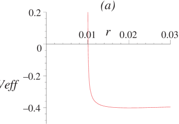
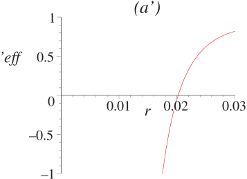
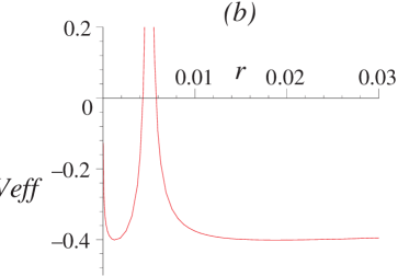
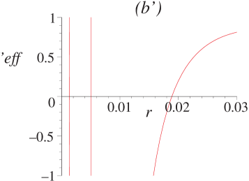
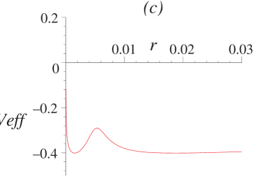
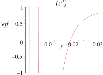
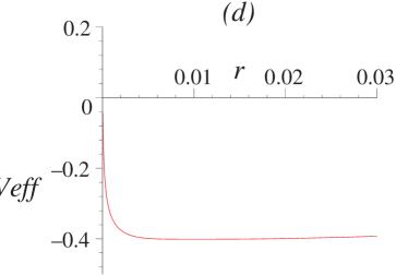
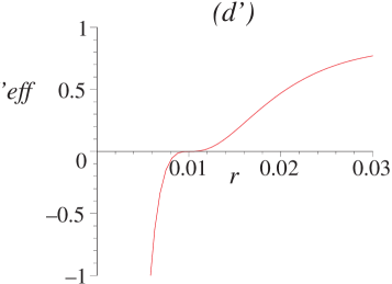
Figure 8: Gravitational features of the D6–brane distribution wrapped on K3 as seen by a neutral test particle. Test particle effective potential (left) and its derivative (right) along the axis of symmetry ($\theta=0$) corresponding to different values of parameter $\ell$: (a) $\ell=0$, (b) $\ell=\ell^{\rm cr}_{\rm r}$, (c) $\ell=\ell^{\rm cr}_{\rm r}+\frac{1}{16}(\ell^{\rm cr}_{\rm e}-\ell^{\rm cr}_{\rm r})$, (d) $\ell=\ell^{\rm cr}_{\rm e}$. For $\ell>\ell^{\rm cr}_{\rm e}$, the effective potential becomes increasingly similar to that of the unwrapped case in figure 5(b). The effective potential is singular (exhibiting infinite repulson) at the singularity radius $r_{\rm r}$. A test particle moving on the equatorial plane ($\theta=\pi/2$) has potential (a) for all values of $\ell$.

On the equatorial plane this is the result of ref.[6], since the solution (24) at $\theta={\pi}/{2}$ reduces to the spherically symmetric solution of $\ell=0$. The test particle feels an attractive force as it approaches from infinity. Attraction would turn into repulsion at the enhançon radius, but at this point we will replace the geometry with a physical one.

For motion along the symmetry axis, the situation is more interesting, as it qualitatively depends on the value of the parameter $\ell$ (see figure 8). In the $\ell=0$ case the physics is much like that described above for the equatorial motion: the potential becomes repulsive inside $r_{\rm e}$ and this repulsion is infinite at $r_{\rm r}$.

For $\ell$ small there are now two enhançon loci. The particle can come from infinity and reach the repulsive region just inside the outer enhançon. This is region II. Alternatively, it can start from the origin (i.e., in region III, where the potential has the same value as at infinity), and be repelled towards the inner enhançon shell. This is the behaviour that we noticed before wrapping the distribution. It is not the repulson geometry which results from wrapping.

For a test particle moving from the origin outwards, the repulson region (resulting from wrapping) starts at the inner enhançon. Now, the repulsive force is directed towards the origin. This situation persists until $\ell=\ell_{\rm r}^{\rm cr}$.

When $\ell>\ell_{\rm r}^{\rm cr}$, a test particle moving along the symmetry axis will still feel a repulsive force, but not an infinite one. In principle, if it had enough energy, it could overcome the potential barrier between inner and outer enhançons and move from infinity to the origin, or vice versa. Still, because the tension of probe branes is still negative in this region, we consider it unphysical and will excise it.

At $\ell=\ell_{\rm e}^{\rm cr}$ the inner and outer enhançon loci meet and the potential barrier vanishes. However, there is still a minimum of the potential, located at $r=\ell=r_{\rm e}$. This minimum persists for $\ell>\ell_{\rm e}^{\rm cr}$, and is located at $r=\ell$, as in the unwrapped case. We stress again that this remaining repulsion has nothing to do with the wrapping, as it is the behaviour observed in the previous section for the unwrapped geometry.

4 Excision

Ultimately, we must remove the parts of the geometry resulting from the wrapping which are unphysical. In order to do this, we must see what sorts of geometry we can replace the bad parts with, ascertaining whether it is consistent to do so. Consistency here will be measured at the level of supergravity, bolstered by intuition from the physics of the underlying string theory.

New stringy physics appears when the volume of the K3 gets to $V_{\star}$. A wrapped D6–brane probe becomes massless there and also delocalises. One cannot place wrapped D6–brane sources in the regions where the volume is less than $V_{\star}$ and so, as in previous cases, the geometry must be, to a good approximation, simply flat space. The junction between the flat space and the well–behaved geometry, (across which the extrinsic curvature will jump, providing a stress tensor source) must be equivalent to a massless brane.

This is the logic that was tested in ref.[6] for the spherically symmetric case with the single prototype shell, and also with additional D2–branes, and further in ref.[18] for the case of geometries made of mixtures of D5– and D1–branes. In these works, it was always spherically symmetric situation under study, but there was a family of concentric enhançon shells of different types, and sometimes non–trivial geometry was grafted in, for consistency. The novelties here are that we have no spherical symmetry, and the nested shells can intersect for some ranges of the parameters, making a toroidal shape. As we shall see, despite this complication, the gravity junction technology[19] allows us to analytically demonstrate that there is a variety of consistent excisions that we can perform.

4.1 A Little Hypersurface Technology

One can perform the excision procedures that were carried out in refs.[6, 18], even though we are far from spherical symmetry, if we are careful about how we set up the problem.

Let our spacetime $M$ have coordinates $x^{\mu}$, and a metric $G_{\mu\nu}$. A general hypersurface $\Sigma$ within $M$ deserves its own coordinates $\xi^{A}$, and so it is specified by an equation of the form $f(x^{\mu}(\xi^{A}))=0$. The unit vector normal to this hypersurface is then specified as

$$n_{\mu}^{\pm}=\mp\sigma\frac{\partial f}{\partial x^{\mu}}\ ,\quad\mbox{where}\,\,\sigma=\left|G^{\mu\nu}\frac{\partial f}{\partial x^{\mu}}\frac{\partial f}{\partial x^{\nu}}\right|^{-1/2}\ .$$ (36)

The induced metric on $\Sigma$ is the familiar

$$G_{AB}=G_{\mu\nu}\frac{\partial x^{\mu}}{\partial\xi^{A}}\frac{\partial x^{\nu}}{\partial\xi^{B}}\ .$$

The main object we shall need is the extrinsic curvature of the surface. This is given by the pullback of the covariant derivative of the normal vector:

$$K_{AB} = \frac{\partial x^{\mu}}{\partial\xi^{A}}\frac{\partial x^{\nu}}{\partial\xi^{B}}\nabla_{\mu}n_{\nu}=-n_{\mu}\left(\frac{\partial^{2}x^{\mu}}{\partial\xi^{A}\partial\xi^{B}}+\Gamma^{\mu}_{\nu\rho}\frac{\partial x^{\nu}}{\partial\xi^{A}}\frac{\partial x^{\rho}}{\partial\xi^{B}}\right)\ .$$ (37)

and is a tensor in the spacetime $\Sigma$. This might seem to be a daunting expression, but (like many things) it simplifies a lot in simple symmetric cases. So in the spherical case, the equation specifying $\Sigma$ is just $f=r-R=0$, for some constant $R$, and we can use the remaining coordinates of $M$ as coordinates on $\Sigma$. Then, $\partial f/\partial r=1$, giving:

$$n_{\mu}^{\pm}=\mp\frac{1}{\sqrt{\left|G^{rr}\right|}}\delta^{r}_{\mu}\ .$$

using the coordinates $\xi^{A}=x^{A}$, we get the simple more commonly used expression:

$$K_{AB}^{\pm}=\mp{1\over 2}\frac{1}{\sqrt{\left|G^{rr}\right|}}{\partial G_{AB}\over\partial r}\ .$$ (38)

In the axially symmetric case, the equation specifying $\Sigma$ is $f=r-R(\theta)=0$, where $R$ is now a function of $\theta$. Since

$$\sigma=|\,G^{rr}+G^{\theta\theta}(\partial_{\theta}R)^{2}|^{-1/2}\ ,$$ (39)

the unit normal vectors are

$$n_{\gamma}^{\pm}=\mp\frac{\delta_{\gamma}^{r}-\delta_{\gamma}^{\theta}\partial_{\theta}R}{\sqrt{|G^{rr}+G^{\theta\theta}(\partial_{\theta}R)^{2}|}}\ .$$ (40)

We can compute the extrinsic curvature:

$$K^{\pm}_{\alpha\beta} = \frac{1}{2}\left(n^{r\pm}\partial_{r}+n^{\theta\pm}\partial_{\theta}\right)G_{\alpha\beta}\ ,$$

$$K^{\pm}_{\theta\theta} = -\,\,n^{\pm}_{r}\partial_{\theta}^{2}R+\frac{1}{2}(n^{r\pm}\partial_{r}G_{\theta\theta}-n^{\theta\pm}\partial_{\theta}G_{\theta\theta})+\,\,\partial_{\theta}R(-n^{r\pm}\partial_{\theta}G_{rr}-n^{\theta\pm}\partial_{r}G_{\theta\theta})$$ (41)

$$\hskip 85.35826pt+\,\,\frac{(\partial_{\theta}R)^{2}}{2}(-n^{r\pm}\partial_{r}G_{rr}+n^{\theta\pm}\partial_{\theta}G_{rr})\ ,$$

where $\alpha,\beta=t,x^{1},...,x^{6},\phi$. This relation will be useful below when we calculate the stress–energy tensor along axially symmetric enhançon shells.

4.2 Torodial Enhançon

We will discuss the toroidal enhançon first. As observed before, the volume of K3 drops below $V_{\star}$ in the interior of the torus. In this region, the metric has the same form as given in equation (4), but we replace $f_{2}$ and $f_{6}$ with new harmonic functions, $h_{2}$ and $h_{6}$. The precise form of these harmonic functions will be determined by the consistency of the theory. Transforming to Einstein frame $G_{\mu\nu}=e^{-{\Phi}/{2}}g_{\mu\nu}$, (this is the natural frame in which to perform this sort of computation) we use the axially symmetric extrinsic curvature (41) to determine the stress–energy tensor along the surface joining our two solutions.

There is a discontinuity in the extrinsic curvature across the junction defined by

$$\gamma_{AB}=K_{AB}^{+}+K_{AB}^{-}\ ,$$

The stress–energy tensor supported at this junction is given by [23]:

$$S_{AB}=\frac{1}{\kappa^{2}}(\gamma_{AB}-G_{AB}\,\gamma_{C}^{C})\ .$$

For our particular geometry, the stress–energy tensor can be computed to be:

$$S_{\mu\nu} = \frac{\sigma}{2\kappa^{2}}(1+\partial_{\theta}R)\left(\frac{f_{2}^{\prime}}{f_{2}}+\frac{f_{6}^{\prime}}{f_{6}}-\frac{h_{2}^{\prime}}{h_{2}}-\frac{h_{6}^{\prime}}{h_{6}}\right)\,\,G_{\mu\nu}\ ,$$

$$S_{ab} = \frac{\sigma}{2\kappa^{2}}(1+\partial_{\theta}R)\left(\frac{f_{6}^{\prime}}{f_{6}}-\frac{h_{6}^{\prime}}{h_{6}}\right)\,\,G_{ab}\ ,$$

$$S_{ij} = 0\ ,$$ (42)

where $\sigma$ has been defined in equation (39) and the prime denotes $\partial/\partial r$. Also, Newton’s constant is set by $2\kappa^{2}=16\pi G_{N}=(2\pi)^{7}(\alpha^{\prime})^{4}g_{s}^{2}$, in the standard units[14]. The indices $a$ and $b$ run over the K3 directions ($x^{3},x^{4},x^{5},x^{6}$), while parallel to the brane’s unwrapped world–volume directions we have indices $\mu,\nu$ which run over the ($t,x^{1},x^{2}$). The transverse directions are labelled by indices $(i,j)$.

As expected, the stress–energy tensor along the transverse directions vanishes, which is consistent with the BPS nature of the system’s constituents. The tension of the discontinuity can be obtained from the components in the longitudinal directions. Recall from equation (35) that $(f_{2}f_{6})^{\prime}=0$ at the enhançon loci given in equation (30). For vanishing tension, then, looking at our result in the middle line of equation (42), we require that $(h_{2}h_{6})^{\prime}$ vanishes at this radius as well. In addition to this constraint, positive tension between the two enhançon shells requires, $V(r,\theta)=Vh_{2}/h_{6}\geq V_{\star}$. If we wish to saturate the bound and assume $h_{2}$ and $h_{6}$ have a similar form to $f_{2}$ and $f_{6}$, the harmonic functions are in fact constant, and a suitable solution is:

$$h_{2} = 1-\frac{(V-V_{\star})}{2V}\ ,$$

$$h_{6} = 1+\frac{(V-V_{\star})}{2V_{\star}}\ .$$ (43)

So we are able to successfully perform the task of cutting out the bad region contained within the toroidal enhançon, replacing it with flat space. It appears that we can have the resulting shell made of zero tension branes, as is in keeping with the intuition about the stringy fate of the constituent branes.

We must note that the “point” $r=0$ is not entirely satisfactory. Indeed, we are justified in thinking of the entire geometry as that of a torus, since in the extended coordinates, this point is really a disc of radius $\ell$. On the edge of this disc, as stated before, the asymptotic volume is ambiguous, but the value $V$ seems to be the most physically consistent, as this is what it is in the disc’s interior. There is no singularity on the disc’s interior, and the volume is not at a special value. This means that there is no requirement to place physical branes there, and so the torus genuinely has a hole in the centre, and not just a single point.

We have ignored the fact that the form of the harmonic function in that region indicates that we might have a negative density of branes on the interior of the disc. We are free to ignore this, since there is no singularity there: the supergravity analysis tells us that we are free to place the zero tension distribution of branes over the whole toroidal surface instead. Of course, there is still the fact that there is repulsion along the symmetry axis as seen by a test particle moving in the geometry. Again, we stress that this behaviour has nothing to do with the wrapping: it is an artifact of the continuous brane distribution we started with. This would not occur for other branes, as we show in section 5.

4.3 Double and Oblate Enhançons

We also have the case $\ell<\ell^{\rm cr}_{\rm e}$, when the enhançon lies in two disconnected parts. We have two choices.

• The first is to simply cut out the entire interior region, and replace it by flat space. This then gives a simple oblate enhançon shape. This is perfectly fine as a solution, and has the extra feature that it gives a case where wrapping removes the entire disc located at $r=0$. This means that this is a case where the enhançon mechanism removes negative tension branes which show up in the unwrapped distribution. In the event that the peculiarities associated to the ring at $r=0$ turn out to be unpalatable, this is a satisfactory conservative choice. It is also the gentlest generalisation from the point of view of the dual moduli space of the gauge theory we shall discuss in section 6.

• We can also keep both the inner and the outer shell, and place flat space in between. This means that the ring is kept again, but then the same words that we used in the case of the toroidal cases apply.

Let us check the supergravity analysis for this case. Recall the three regions defined in section 3. Region II represented the unphysical geometry where the tension of a brane probe becomes negative. It contains the repulson singularity. We can perform an incision as was done for the toroidal enhançon by defining $h_{2}$ and $h_{6}$ as above, between the two enhançon shells. The geometry of regions I and III are consistent and can be defined as in equations (4). We can alternatively define the harmonic functions in region III to be

$$f_{2} \to \tilde{f}_{2}=1-\frac{r_{6}^{\prime}}{r\Delta}\frac{V_{\star}}{V}\ ,$$

$$f_{6} \to \tilde{f}_{6}=1+\frac{r_{6}^{\prime}}{r\Delta}\ .$$ (44)

where $r_{6}^{\prime}\leq r_{6}$. The double enhançon, then, allows for some number $N^{\prime}\leq N$ of wrapped D6–branes in the interior of our geometry.

If we perform the excision, the stress–energy tensor for the outer shell is as in equation (42) where $R$ is the outer enhançon radius. The inner shell has a stress energy tensor given by:

$$S_{\mu\nu} = \frac{\sigma}{2\kappa^{2}}(1+\partial_{\theta}\tilde{R})\left(\frac{h_{2}^{\prime}}{h_{2}}+\frac{h_{6}^{\prime}}{h_{6}}-\frac{\tilde{f}_{2}^{\prime}}{\tilde{f}_{2}}-\frac{\tilde{f}_{6}^{\prime}}{\tilde{f}_{6}}\right)\,\,G_{\mu\nu}\ ,$$

$$S_{ab} = \frac{\sigma}{2\kappa^{2}}(1+\partial_{\theta}\tilde{R})\left(\frac{h_{6}^{\prime}}{h_{6}}-\frac{\tilde{f}_{6}^{\prime}}{\tilde{f}_{6}}\right)\,\,G_{ab}\ ,$$

$$S_{ij} = 0\ .$$ (45)

Here $\tilde{R}(\theta)$ is the equation (30) of the inner enhançon shell defined in terms of $r_{6}^{\prime}$. Again, the transverse stresses vanish and the tension vanishes at the inner enhançon shell.

So, we see that we have constructed a geometry which is consistent with supergravity and excises the unphysical negative tension brane geometry resulting from wrapping.

In the case of the double shell enhançon geometry, one might wonder how such a geometry can be constructed. Consider probing our geometry with $n_{2}$ D2–branes as was done in refs.[18, 6, 5]. Such branes are able to pass through the enhançon shells since they are not wrapped on the K3 and so their tension remains positive. This is evident from the effective Lagrangian

$${\cal L}=n_{2}\tau_{2}f_{6}\,\,\frac{1}{2}v^{2}\ .$$ (46)

We can additionally probe our geometry with $n$ D2–D6 bound states, as discussed in ref.[18]. The effective Lagrangian is given by:

$${\cal L}=n\tau_{6}Vf_{2}\,\,\frac{1}{2}v^{2}\ .$$ (47)

The presence of the bound D2–brane ensures that the volume of K3 does not drop below $V_{\star}$. The bound state can therefore pass through the outer enhançon shell and continue on to the origin.

Once we are in the interior, region III, we can separate the D2–branes from the D6–branes since the K3 volume is greater than $V_{\star}$ there. The D6–branes have positive tension and hence are free to move about in the interior. If we attempt to move a D6–brane out of region III, the volume of K3 approaches $V_{\star}$ as the brane nears the inner enhançon shell. The D6–brane becomes tensionless at the inner enhançon and melts into the shell, as happens for brane approaching the outer shell from outside. Hence, D2–D6 bound states can be used to move D6–branes into the interior and to add D6 branes to the inner enhançon shell. It is easy to imagine building the double shell enhançon geometry in this fashion, starting with widely separated D2– and D6–branes, and then removing the D2–branes after the construction.

5 Wrapping Other Distributed D–Branes

We focused on D6–branes almost exclusively, but it should be clear that many of the amusing features that we have seen are also present for wrapping D4– and D5– branes. In fact, we ought to stress again here that the possibly unpalatable feature of the negative brane density and its repulsive potential are not generic. (We have already seen that the disc brane distributions for all of the other branes have positive densities everywhere.)

The feature of having multiple solutions for the enhançon locus will occur also. In fact, it will give up to three solutions for the D4–brane’s enhançon loci, but only one for the D5–brane. This is because the harmonic functions will be of the form:

$$f=1+\frac{r_{p}^{7-p}}{r^{7-p}\left(1+({\ell^{2}}/{r^{2}})\cos^{2}\theta\right)}\ .$$

for $p=4,5$ and one non–zero parameter $\ell_{1}=\ell$. The equation determining the enhançon loci is of the form of equating a ratio of two of these $f$’s to a constant, $V_{\star}/V$ which gives a quadratic equation in the case of the D6–brane, as we have seen, but only a linear equation for D5–branes. The D4–brane case will give a cubic equation.

5.1 Unwrapped D5–Brane Distributions

Actually, it is worth looking briefly a bit more at the D5–brane case, keeping non–zero both of the parameters, $\ell_{1},\ell_{2}$, that we can have with four transverse directions. Taking the extremal limit of the rotating black D5–brane solution given in ref.[13] we get for our unwrapped solution:

$$ds^{2} = f_{5}^{-1/2}\Big{(}-dt^{2}+\sum_{i=1}^{5}dx_{i}^{2}\Big{)}$$

$$\hskip 85.35826pt+f_{5}^{1/2}\Big{(}\frac{\Delta_{12}}{\Xi_{1}\Xi_{2}}dr^{2}+\Delta_{12}r^{2}d\theta^{2}+\Xi_{1}r^{2}\sin^{2}\phi_{1}+\Xi_{1}r^{2}\cos^{2}\phi_{2}\Big{)}\ ,$$

$$e^{\Phi} = f_{5}^{-1/2}\ ,$$

$$C_{6} = f_{5}^{-1}dt\wedge dx_{1}\wedge\ldots\wedge dx_{5}\ ,$$ (48)

where

$$f_{5}=1+\frac{r_{5}^{2}}{r^{2}\Delta_{12}}\ ,$$

and

$$\Delta_{12}=1+\frac{\ell_{1}^{2}}{r^{2}}\cos^{2}\theta+\frac{\ell_{2}^{2}}{r^{2}}\sin^{2}\theta\ ,\qquad\Xi_{1}=1+\frac{\ell_{1}^{2}}{r^{2}}\ ,\qquad\Xi_{2}=1+\frac{\ell_{2}^{2}}{r^{2}}\ .$$

The extended coordinates are given by:

$$y_{1} = \sqrt{r^{2}+\ell_{1}^{2}}\sin\theta\cos\phi_{1}\ ,\qquad y_{2}=\sqrt{r^{2}+\ell_{1}^{2}}\sin\theta\sin\phi_{1}\ ,$$

$$y_{3} = \sqrt{r^{2}+\ell_{2}^{2}}\cos\theta\cos\phi_{2}\ ,\qquad y_{4}=\sqrt{r^{2}+\ell_{2}^{2}}\cos\theta\sin\phi_{2}\ .$$

Considering the case $\ell_{1}=\ell,\ell_{2}=0$ will give the ring density mentioned previously.

Let us consider particle probes of the geometry. Previously we associated repulsive gravitational features of the D6–brane distribution with a negative brane density on the disc. The D5–brane distribution did not have negative brane density, and indeed, does not show these repulsive features. In this case the transverse space–time has one more dimension, but it is also endowed with one additional Killing vector related to the $\phi_{2}$ coordinate. Therefore an analysis similar to the one set forth in section 2.1 shows that test particle motion in $\theta=0$ and $\theta=\pi/2$ directions is governed by the same effective potential given in equation (23). In fact, the effective potential in the $\theta=0$ direction does depend only on $\ell_{1}$ and in the $\theta=\pi/2$ direction only on $\ell_{2}$, while the form of dependence is identical. As figure 9 shows, the repulsive gravitational features are completely absent.

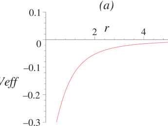
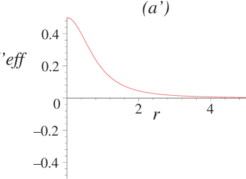
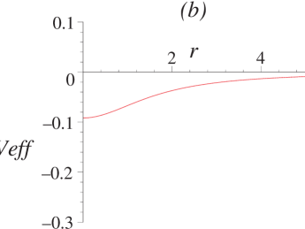
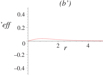
Figure 9: Gravitational features of the distributed D5–brane solution as seen by a neutral test particle. Test particle effective potential (left) and its derivative (right) along the $\theta=0$ ($\theta=\pi/2$) direction corresponding to (a) $\ell_{1}=0$ ($\ell_{2}=0$), (b) $\ell_{1}>0$ ($\ell_{2}>0$). The potential is always attractive for a particle moving in from the infinity.

5.2 Wrapped D5–Brane Distributions

Wrapping the D5–brane configuration (5.1) on K3 yields

$$ds^{2} = f_{5}^{-1/2}f_{1}^{-1/2}\big{(}-dt^{2}+dx^{2}\big{)}+f_{5}^{-1/2}f_{1}^{1/2}Vds_{K3}^{2}$$

$$+f_{5}^{1/2}f_{1}^{1/2}\Big{(}\frac{\Delta_{12}}{\Xi_{1}\Xi_{2}}dr^{2}+\Delta_{12}r^{2}d\theta^{2}+\Xi_{1}r^{2}\sin^{2}\phi_{1}+\Xi_{1}r^{2}\cos^{2}\phi_{2}\Big{)}\ ,$$

$$e^{\Phi} = f_{5}^{-1/2}f_{1}^{1/2}\ ,$$

$$C_{6} = f_{5}^{-1}dt\wedge dx\wedge Vds_{K3}\ ,$$

$$C_{2} = f_{1}^{-1}dt\ ,\wedge dx$$ (49)

where

$$f_{5}=1+\frac{r_{5}^{2}}{r^{2}\Delta_{12}}\ ,\qquad f_{1}=1-\frac{r_{1}^{2}}{r^{2}\Delta_{12}}\ ,\qquad r_{1}^{2}=\frac{V_{\star}}{V}r_{5}^{2}\ ,$$

and $\Delta_{12}$, $\Xi_{1}$, $\Xi_{2}$, etc., defined as before. There is a repulson singularity at

$$r_{\rm r}=\sqrt{\frac{r_{5}^{2}V_{\star}}{V}\Big{(}1-\frac{V}{r_{5}^{2}V_{\star}}(\ell_{1}^{2}\cos^{2}\theta+\ell_{2}^{2}\sin^{2}\theta)\Big{)}}\ ,$$

where the running volume of K3 shrinks to zero. Interestingly, the singularity disappears completely when both parameters $\ell_{1}$ and $\ell_{2}$ exceed the critical value

$$\ell^{\rm cr}_{\rm r}=\sqrt{\frac{r_{5}^{2}V_{\star}}{V}}\ .$$

The singularity is always surrounded by the enhançon shell at

$$r_{\rm e}=\sqrt{\frac{2r_{5}^{2}V_{\star}}{V-V_{\star}}\Big{(}1-\frac{V-V_{\star}}{2r_{5}^{2}V_{\star}}(\ell_{1}^{2}\cos^{2}\theta+\ell_{2}^{2}\sin^{2}\theta)\Big{)}}\ .$$

Depending on the values of $\ell_{1}$ and $\ell_{2}$, this enhançon assumes various shapes, but is always connected. Again, it is interesting that when both parameters $\ell_{1}$ and $\ell_{2}$ exceed the critical value

$$\ell^{\rm cr}_{\rm e}=\sqrt{\frac{2r_{5}^{2}V_{\star}}{V-V_{\star}}}\ ,$$

the enhançon disappears completely. See figure 10 for a series of snapshots.

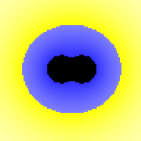
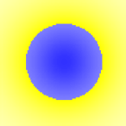
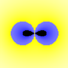
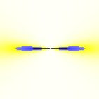
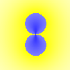
Figure 10: Some two–dimensional slices through the non–spherical wrapped D5–brane geometry before excision. $\theta=0$ corresponds to the vertical direction and $\theta=\pm{\pi}/{2}$ to the horizontal. The configuration is symmetric in $\phi_{1}$ and $\phi_{2}$ (not shown on the figure). The colour coding is as in figure 6. The shapes vary for different values of the parameters $\ell_{1}$ and $\ell_{2}$: $\ell_{1}=\ell_{2}=0$ (top, left), $\ell_{1}=\frac{7}{8}\ell^{\rm cr}_{\rm r}$, $\ell_{2}=0$ (top, second), $\ell_{1}=0$, $\ell_{2}=\ell^{\rm cr}_{\rm r}$ (top, third), $\ell_{1}=\ell_{2}=\ell^{\rm cr}_{\rm r}$ (top, right), $\ell_{1}=\ell^{\rm cr}_{\rm e}$, $\ell_{2}=0$ (bottom, left) $\ell_{1}=8\ell^{\rm cr}_{\rm e}$, $\ell_{2}=0$ (bottom, second) $\ell_{1}=\ell^{\rm cr}_{\rm r}$, $\ell_{2}=\ell^{\rm cr}_{\rm e}$ (bottom, third) $\ell_{1}=\ell_{2}=\ell^{\rm cr}_{\rm e}-\frac{1}{16}(\ell^{\rm cr}_{\rm e}-\ell^{\rm cr}_{\rm r})$ (bottom, right).

It is important to note that the following result is true

$$\frac{\partial}{\partial r}\Big{(}f_{5}f_{1}\Big{)}\Big{|}_{r=r_{\rm e}}=0\ .$$ (50)

It is this that will ensure that the supergravity matching computation will go through in a similar manner as in the D6–branes case here, and as in the D5–brane cases studied in ref.[18].

Let us consider particle probes again, in order to check where the repulsive regions are. In contrast to the D6–brane case, we do not expect any repulsive features to arise which are not attributable to the wrapping. The presence of the repulson singularity is signalled by a singularity in the effective potential occurring at $r_{\rm r}$. This is surrounded by the enhançon shell, residing precisely at the minimum of the potential, i.e., where the repulsive region starts. (See figure 11.) There is still some residual finite repulsion even after $\ell_{1}$ ($\ell_{2}$) exceeds $\ell^{\rm cr}_{\rm r}$ and the repulson singularity disappears (figure 11(c)). Beyond $\ell_{1}>\ell^{\rm cr}_{\rm e}$ ($\ell_{2}>\ell^{\rm cr}_{\rm r}$) the effective potential becomes completely attractive with a minimum at the origin $r=0$.

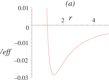
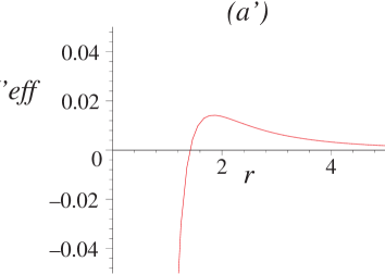
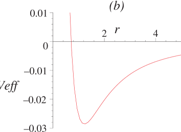
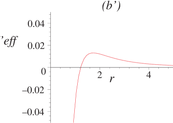
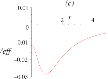
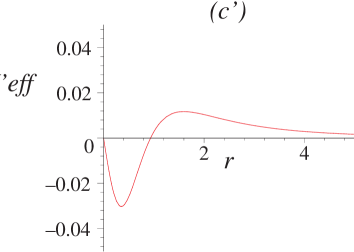
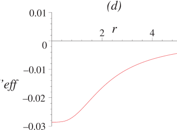
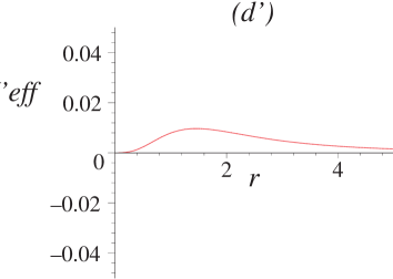
Figure 11: Gravitational features of the distributed D5–brane solution wrapped on K3 as seen by a neutral test particle. Test particle effective potential (left) and its derivative (right) along the $\theta=0$ ($\theta=\pi/2$) direction corresponding to (a) $\ell_{1}=0$ ($\ell_{2}=0$), (b) $\ell_{1}=\ell^{\rm cr}_{\rm r}$ ($\ell_{2}=\ell^{\rm cr}_{\rm r}$), (c) $\ell_{1}=\ell^{\rm cr}_{\rm r}+\frac{1}{2}(\ell^{\rm cr}_{\rm e}-\ell^{\rm cr}_{\rm r})$, ($\ell_{2}=\ell^{\rm cr}_{\rm r}+\frac{1}{2}(\ell^{\rm cr}_{\rm e}-\ell^{\rm cr}_{\rm r})$), (d) $\ell_{1}=\ell^{\rm cr}_{\rm e}$ ($\ell_{1}=\ell^{\rm cr}_{\rm e}$). Effective potential is singular (exhibiting infinite repulson) at $r_{\rm r}$ and has a minimum at $r_{\rm e}$.

6 Gauge Theory

It is worth remembering that some of our results pertain to gauge theory. Wrapping the D6–branes on the K3 results in an ${\cal N}=4$ $(2+1)$–dimensional gauge theory with UV gauge coupling[1, 14]:

$$g^{2}_{\rm YM}=(2\pi)^{4}g_{s}\alpha^{\prime 3/2}V^{-1}\ .$$

One of the results that one can readily extract from the analysis of the spherical case[1] is the piece of the gauge theory moduli space corresponding to the movement of a single wrapped probe. In gauge theory, this is the metric derived from the kinetic terms in the low energy effective action for the field breaking $SU(N)\to SU(N-1)\times U(1)$. The probe computation yields the tree level and one–loop contribution to this result, and there are no perturbative corrections.

In the present case, we should be able to see new physics, since the parameter $\ell$ should have some meaning in the gauge theory. In fact, we expect that it should be controlling the vacuum expectation value of an operator made by the symmetric product of the adjoint scalars, by analogy with the case in the AdS/CFT[24, 25] context. Here, the $R$–symmetry is $SU(2)\simeq SO(3)$. The three adjoint scalars in the gauge multiplet, transforming as the ${\bf 3}$, can be combined by symmetric product. The $R$–charge of the resulting operator is computed in the usual way. For example, ${\bf 3}\times{\bf 3}$=${\bf 1}+{\bf 5}+{\bf 3}$, where the ${\bf 5}$ is the symmetric traceless part. This is of course more familiar as the $j=2$ case in the standard angular momentum notation where the irreducible representations of the $R$–symmetry group are written as $2j+1$ dimensional. We should see some sign of this show up here, and indeed we do.

6.1 Metric on Moduli Space

We probe the repaired geometry with a single wrapped D6–brane in order to extract the data of interest. After including the $U(1)$ world–volume gauge sector into the probe calculation, dualising the gauge field to get the extra periodic scalar[1, 14], the kinetic term of the effective action in the non–flat regions becomes

$$T=h(r,\theta)\,\,\left(\frac{\Delta}{\Xi}\,{\dot{r}^{2}}+\Delta r^{2}\,\dot{\theta}^{2}\ +\Xi\,r^{2}\sin^{2}\theta\,\dot{\phi}^{2}\right)+h(r,\theta)^{-1}\left(\dot{s}/2-\mu_{2}C_{\phi}\dot{\phi}/2\,\right)^{2}.$$

where $h(r,\theta)$ is defined by

$$h(r,\theta)=\frac{\mu_{6}}{2}\,(Vf_{2}-V_{\star}f_{6})$$

and $C_{\phi}$ is the magnetic potential corresponding to the D6–brane charge

$$C_{\phi}=-r_{6}\ \frac{\Xi}{\Delta}\cos\,\theta\ .$$

To extract the gauge theory we work with variables[24]:

$$U=\frac{r}{\alpha^{\prime}}\ ,\quad a=\frac{l}{\alpha^{\prime}}\ ,$$

and take the decoupling limit, which involves holding $U,\ a,$ and $g_{YM}^{2}$ fixed while taking $\alpha^{\prime}\to 0$. The metric becomes:

$$ds^{2}=h(U,\theta)\ \left(\frac{\Delta^{\prime}}{\Xi^{\prime}}\,dU^{2}+\Delta^{\prime}U^{2}\,d\theta^{2}\ +\Xi^{\prime}\,U^{2}\sin^{2}\theta\,d\phi^{2}\right)+h(U,\theta)^{-1}\left(d\sigma-\frac{N}{8\pi^{2}}A_{\phi}d\phi\,\right)^{2}\ ,$$

with

$$h(U,\theta)=\frac{1}{8\pi^{2}g^{2}_{YM}}\left(1-\frac{g^{2}_{YM}N}{U\Delta^{\prime}}\right)\ .$$

Here we have defined

$$\Delta^{\prime}=1+\frac{a^{2}}{U^{2}}\cos^{2}\theta\ ,\quad\Xi^{\prime}=1+\frac{a^{2}}{U^{2}}\ ,$$

and

$$\sigma=\frac{s\alpha^{\prime}}{2}\ ,\quad A_{\phi}=-\frac{1}{2}\frac{\Xi^{\prime}}{\Delta^{\prime}}\cos\theta\ .$$

This might not seem terribly inspiring, but recall that we can work in the extended coordinate system given by the obvious generalisation of equation (6):

$$W_{1} = \sqrt{U^{2}+a^{2}}\,\sin\theta\,\cos\phi$$

$$W_{2} = \sqrt{U^{2}+a^{2}}\,\sin\theta\,\sin\phi$$

$$W_{3} = U\,\cos\theta.$$ (51)

In terms of these, our moduli space result is the standard Taub–NUT form:

$$ds^{2}=H(W,{\hat{\theta}})\ \left(d\vec{W}\cdot d\vec{W}\right)+H(W,{\hat{\theta}})^{-1}\left(d\sigma-\frac{N}{8\pi^{2}}A_{\phi}d{\phi}\,\right)^{2}\ ,$$ (52)

with

$$H(W,{\hat{\theta}})=\frac{1}{8\pi^{2}g^{2}_{YM}}\left(1-\frac{g^{2}_{YM}N\sqrt{\Lambda+\Sigma}}{\sqrt{2}\Sigma}\right)\ .$$

where

$$\Sigma=\sqrt{\Lambda^{2}+4a^{2}W_{3}^{2}},\qquad\Lambda=W^{2}-a^{2},\qquad W=\sqrt{W_{1}^{2}+W_{2}^{2}+W_{3}^{2}}\ .$$

The content is in the harmonic function, and we can expand it for large $W$ using our earlier observations in equations (19):

$$H = \frac{1}{8\pi^{2}g^{2}_{YM}}\left(1-\frac{g^{2}_{YM}N}{W}\sum_{n=0}^{\infty}(-1)^{n}\left(\frac{a}{W}\right)^{2n}P_{2n}(\cos\ \hat{\theta})\right)\ ,$$ (53)

where we have defined new polar coordinate angles in an analogous manner to that shown in equation (20), and the $P_{2n}(x)$ are the Legendre polynomials in $x$, as before (see equation (21)).

The leading terms in this large $W$ expansion should have an interpretation as the contribution of the operators which are switched on. The $n=0$ result is that of the spherical case[1]. The case $n=1$ comes with the Legendre polynomial $P_{2}(\cos{\hat{\theta}})$, which has the $R$–charge of the ${\bf 5}$, the simplest operator one can make out the adjoint scalars. So the parameter $\ell$, (i.e., $a$) controls the vacuum expectation value of this operator, with subleading contributions coming from the higher spherical harmonics.

Notice that this expansion is not sensitive to some of choices that we can make in doing the excision. In particular, while it works for any $\ell$, it is for large $y$. So from the point of view of this expansion, all of the choices are equivalent to the excisions which give a single locus: For $\ell<\ell_{\rm e}^{\rm cr}$, this is the oblate enhançon with flat space inside, while for $\ell>\ell_{\rm e}^{\rm cr}$, it is the toroidal shape. The difference between the two is presumably non–perturbative in the operator expansion. It would be interesting to find gauge theory meaning for cases where we can choose to have a double shell.

7 Concluding Remarks

We have seen that enhançon shapes quite different from the prototype spherical case can be well described within supergravity. We achieved this by wrapping distributions of D–branes on K3, and uncovered many interesting and beautiful features of the resulting geometry.

While the main example we used here (the D6–brane distribution) had a physical oddity at its core (a negative contribution to the brane density), we continued to use it as out main example, since it is clear that this feature does not affect the discussion of the enhançon. Indeed, we showed that all of the salient features we wanted to illustrate are present for D5–brane distributions, (and very likely also extend to D4–branes) which do not have any such problems with the distribution’s density. For the D5–branes in fact, it is clear that the excision process always removes the original disc distribution of branes (this time they are all on the edge), and so the problem in that case is moot.

In fact, it would be interesting to study our D6–brane distribution further to determine if there is some mechanism, perhaps similar to the enhançon, which might resolve the apparently unphysical features (repulsive force and negative brane density) that we observed. This odd behaviour may be a residual effect inherited from the fully rotating configuration since we are studying an extremal limit of that solution. Perhaps a consideration of the full solution will provide additional insight.

We were able to use the geometry to extract some quite interesting new information about the associated $SU(N)$ gauge theory whose moduli space is isomorphic to that of the wrapped D6–brane problem. One can read off the details of which operator vacuum expectation values have been switched on from an expansion of a probe result in terms of spherical harmonics. Of course, similar results for other gauge groups should be easily extracted by a generalisation of the work of ref.[26] along the lines done here.

Overall, it is very satisfying that we can find and exactly analyse such intricate structures, successfully correcting poorly behaved supergravity geometries with knowledge from the underlying string theory. This is encouraging, since such studies have potential applications to searches for realistic gauge/geometry duals, better understanding of singularities in string theory, and a host of other inter–related problems.

References

- [1] C. V. Johnson, A. W. Peet and J. Polchinski, Phys. Rev. D 61, 086001 (2000), [hep-th/9911161].
-
[2]
K. Behrndt,
Nucl. Phys. B 455, 188 (1995), [hep-th/9506106];
R. Kallosh and A. D. Linde, Phys. Rev. D 52, 7137 (1995), [hep-th/9507022];
M. Cvetic and D. Youm, Phys. Lett. B 359, 87 (1995), [hep-th/9507160]. - [3] E. B. Bogomolny, Sov. J. Nucl. Phys. 24, 449 (1976) [Yad. Fiz. 24, 861 (1976)].
- [4] C. V. Johnson, Phys. Rev. D 63, 065004 (2001), [hep-th/0004068].
- [5] C. V. Johnson, Int. J. Mod. Phys. A 16, 990 (2001), [hep-th/0011008].
- [6] C. V. Johnson, R. C. Myers, A. W. Peet and S. F. Ross, Phys. Rev. D 64, 106001 (2001), [hep-th/0105077].
- [7] K. Maeda, T. Torii, M. Narita and S. Yahikozawa, hep-th/0107060.
- [8] D. Astefanesei and R. C. Myers, “A New Wrinkle on the Enhançon”, hep-th/0112133.
- [9] M. Wijnholt and S. Zhukov, hep-th/0110109.
- [10] P. Kraus, F. Larsen and S. P. Trivedi, JHEP 9903, 003 (1999), [hep-th/9811120].
- [11] K. Sfetsos, JHEP 9901, 015 (1999), [hep-th/9811167].
- [12] J. G. Russo, Nucl. Phys. B 543, 183 (1999), [hep-th/9808117].
- [13] T. Harmark and N. A. Obers, JHEP 0001, 008 (2000), [hep-th/9910036].
- [14] C. V. Johnson, “D-brane Primer”, hep-th/0007170.
- [15] G. T. Horowitz and A. Strominger, Nucl. Phys. B 360, 197 (1991).
- [16] D. Z. Freedman, S. S. Gubser, K. Pilch and N. P. Warner, JHEP 0007, 038 (2000), [hep-th/9906194].
- [17] A. A. Tseytlin, Mod. Phys. Lett. A 11, 689 (1996), [hep-th/9601177].
- [18] C. V. Johnson and R. C. Myers, Phys. Rev. D 64, 106002 (2001), [hep-th/0105159].
-
[19]
G. Darmois, Memorial de Sciences Mathematiques,
Fascicule XXV, “Les equations de la gravitation
einsteinienne”, Chapitre V (1927);
W. Israel, Nuovo Cimento, B44, 1 (1966); Erratum: ibid., B44, 463. - [20] P. Musgrave and K. Lake, Class. Quant. Grav. 13, 1885 (1996), [gr-qc/9510052].
- [21] S.P. Drake and R. Turolla, Class. Quant. Grav. 14, 1883 (1997), [gr-qc/9703084].
- [22] R. Mansouri and M. Khorrami, J. Math. Phys. 37, 5672 (1996), [gr-qc/9608029].
- [23] C. Lanczos, Phs. Z. 23, 539 (1922); Ann. Phys. (Leipzig) 74 518 (1924).
- [24] J. Maldacena, Adv. Theor. Math. Phys. 2, 231 (1998) [Int. J. Theor. Phys. 38, 1113 (1998)], [hep-th/9711200].
-
[25]
S. S. Gubser, I. R. Klebanov and A. M. Polyakov,
Phys. Lett. B 428, 105 (1998), [hep-th/9802109];
E. Witten, Adv. Theor. Math. Phys. 2, 253 (1998), [hep-th/9802150]. - [26] L. Järv and C. V. Johnson, Phys. Rev. D 62, 126010 (2000), [hep-th/0002244].